@

We propose a new field-theoretic framework for formulating the non-relativistic quantum mechanics of D particles (D0 branes) in a Fock space of U($N$) Yang-Mills theories with all different $N$ simultaneously. D-particle field operators, which create and annihilate a D particle and hence change the value of $N$ by one, are defined. The base space of these D particle fields is a (complex) vector space of infinite dimension. The gauge invariance of Yang-Mills quantum mechanics is reinterpreted as a quantum-statistical symmetry, which is taken into account by setting up a novel algebraic and projective structure in the formalism. Ordinary physical observables of Yang-Mills theory, obeying the standard algebra, are expressed as bilinear forms of the D-particle fields. Together with the open-closed string duality, our new formulation suggests a trinity of three different but dual viewpoints of string theory.

1. Introduction

The idea of a quantized field is a precise expression of the primordial duality between waves and particles in quantum theory. Historically, it stemmed from the quantization of the classical electromagnetic field on the side of waves, while on the particle side from the second quantization of the configuration-space formulation of non-relativistic particle quantum mechanics. As a unification of two classically different concepts, the notion of a quantized field should be taken as more fundamental than its ancestors. It is therefore natural that string field theory [1, 2, 3, 4] has been developed from the early days of string theory towards its non-perturbative formulation. Indeed, even though during the first two decades of their initial development the various versions of string field theory represent mere rewritings of the world-sheet CFT dynamics of strings in terms of ordinary Feynman rules, the situation has been changing in recent years: String field theory, especially the version of open-string field theories first proposed in the seminal work Ref.[2], is now playing an important role in the studies of some crucial aspects of non-perturbative string physics, such as tachyon condensation, albeit still at a classical level [5].

With the advent of D-branes, it became recognized that the natures of open and closed string field theories are quite different: Open strings, and hence open-string fields, should be understood as the collective degrees of freedom for describing D-branes, while closed strings are the bulk degrees of freedom corresponding to gravitons and their partners for which D-branes can be regarded as sources or as soliton-like objects. In closed string field theory, they can emerge as classical solutions (with or without sources) for the equations of motion. In principle, these two descriptions must be connected through the duality between open and closed strings, and constitute a foundation for gauge-gravity correspondence. However, there has been only limited success in formulating the open-closed string duality from this viewpoint. For example, it has not been clarified how to extract the bulk degrees of freedom of closed strings concretely from open-string field theory and vice versa, although some suggestive properties have been discovered, such as those related to lump solutions, to be interpreted as D-branes in the proposal of the so-called ‘vacuum’ string field theory [6] in bosonic string theory.

In ordinary local quantum field theory, it is well known that there is an analogous phenomenon , which provides us a clear and rigorous example of a duality related to solitons. That is the duality [7] between the massive Thirring model and the sine-Gordon model in two-dimensional spacetime. In this case, the kink (and anti-kink) solitons of the latter are described by a massive Dirac field whose interaction is described by the non-linear 4-fermi term in the former. These two descriptions can be translated into each other in both directions through bosonization or fermionization. It should also be mentioned that in two dimensions the massless QED, the Schwinger model [8], provides a suggestive analog to the open-closed string duality, in the sense that the one-loop quantum effect of the massless Dirac field gives a pole singularity corresponding to a composite massive scalar field. This is reminiscent of the phenomenon that the one-loop amplitudes of open strings give rise to pole singularities associated with the propagation of a closed string.

In these examples of the formulations of duality, it is crucial that the soliton degrees of freedom are treated as a quantized field, namely as the Dirac field for which the bosonization gives the sine-Gordon field (or the free massive scalar field in the case of the Schwinger model). The Dirac field corresponds to D-branes described collectively by open strings, while the elementary bosonic fields, as the analog of a closed string field, are obtained from bilinear forms of the Dirac field.

These considerations provide motivation for attempting to construct a certain field-theory-like formalism for treating D-branes, in the hope of clarifying the fundamental open-closed string duality and thereby seeking new languages for non-perturbative string/M physics. It seems worthwhile to explore the possibility of field operators creating and annihilating D-branes, within the setup of the Fock space of D-branes. Although some of the mathematical ideas usually employed in describing D-branes, such as the K-theory approach, involve certain aspects of changing the number of D-branes (and anti-D-branes) from the viewpoint of their topological properties, they do not seem from a physics viewpoint to be concrete enough as a formalism of treating real dynamics. The purpose of the present work is to initiate a more physical approach, introducing D-brane field operators explicitly. We hope to take a first step towards our goal by treating the case of D0-branes, D-particles, within the low-energy approximation such that they are properly described by U($N$) (super) Yang-Mills quantum mechanics [9]. Note that the open-string field theory with Chan-Paton symmetry and Yang-Mills quantum mechanics as its low-energy effective theory are both first-quantized formulations for D particles, though they are second-quantized theories from the viewpoint of open strings. Thus, we introduce the Fock space of the Yang-Mills theory in $0+1$ dimensions by treating all the different $N$ in a completely unified way. We can think of many desirable extensions, for example, including anti-D-branes and covariantizating the formalism both in 10 and 11 dimensions [10] in the context of M-theory. Such attempts would perhaps require the inclusion of all massive degrees of freedom of open strings. This is left hopefully for future works.

In the literature of D-brane Yang-Mills theories, it has been claimed that the Yang-Mills quantum mechanics is already second-quantized. However, in precise terms, this is not true, since Yang-Mills quantum mechanics is yet a configuration-space formulation of D particles, in which the basic degrees of freedom are matrix variables whose diagonal components represent nothing but the coordinates of D particles. Also, by a ‘second’ quantization of Yang-Mills theory, one might imagine to introduce just a collection of symmetrized tensor products of an arbitrary number of Hilbert spaces of the same Yang-Mills theory. However, this is not what we want, as will become evident through our discussion given in the next section.

In a previous work [11], the present author discussed a similar question in the case of D3-branes within the restriction of the 1/2-BPS condition. Unfortunately, however, under the latter condition, we could only deal with the two-point correlation functions (and the so-called extremal correlators) of a special class of operators which are protected from interactions. In the present work, we do not require such additional restrictions, other than the low-energy approximation and the exclusion of anti-D particles. Thus the situation is quite different from that of the previous work. Yet there is an important lesson which we shall follow in the present work. We expect an entirely new mathematical structure for treating D-brane fields. The reason for this is, as we discuss in detail in the following sections, that the symmetry of the configuration-space formulation underlying multi-D-brane states is not the permutation symmetry of usual multi-particle quantum mechanics. Rather, it must be replaced by the U($N$) gauge symmetry of Yang-Mills theory. In other words, D-branes can be treated neither as ordinary bosons nor fermions, and their fields do not have any classical counterparts. From the viewpoint of ordinary quantum field theory, this is a drastic leap, which forces us to go beyond the standard framework of quantum field theory. What we explore in the following is mainly the problem of how to deal with such a quantum system with a continuous statistical symmetry. As we argue, this requires that we invent a novel structure for the operator algebra of D-particle fields, which to the author’s knowledge has never been conceived.

This paper is organized as follows. In section 2, we discuss the problems related to the continuous statistical symmetry and explain our approach for separating the matrix degrees of freedom such that they are suitable for the idea of a Fock space of Yang-Mills theory with all different $N$. We then introduce D-particle field operators and explain their novel properties, which are clearly beyond the ordinary canonical framework of quantum field theories. In section 3, we show how to construct various physical observables corresponding to the gauge invariant operators of Yang-Mills theory as bilinear forms of the D-particle fields. As many of our concepts and notation must be entirely alien to the reader, some elementary details of the calculation are presented in the text for the purpose of avoiding confusion. In a first reading, the reader may skip these details of the calculations. The extension of the present formalism to the case of super Yang-Mills theory is discussed briefly in section 4. Finally, section 5 is devoted to concluding remarks.

2. The Fock space of D-particle quantum mechanics

2.1 Preliminaries

In trying to formulate a second-quantized field theory of D-branes whose fundamental degrees of freedom in the first-quantized formulation are matrix variables, one of the puzzling questions is how to deal with gauge symmetry. We need a unified treatment for all sizes of matrices. A typical case among those with which we are already familiar is the $c=1$ matrix model with a single Hermitian $N\times N$ matrix variable $X_{ab}(t)$, restricted to its singlet sector. In this case, we can first diagonalize the matrix variable and treat the $N$ eigenvalues $\lambda_{a}$ as independent degrees of freedom, whereby the residual gauge symmetry is reduced to the permutation symmetry of the eigenvalues. Then, by taking into account the gauge-volume factor, the Vandelmonde determinant, originating in the integration measure for the matrix variable, the model can be treated as a system of $N$ free fermions whose coordinates are those eigenvalues. Thus, in this particular example, the problem of second-quantizing matrix systems with all different $N$ is reduced to the standard one. It is shown in [11] that this mechanism can be extended to all the SO($6$) multiplets of 1/2-BPS operators of ${\cal N}=4$ SYM₄ if we associate the SO($6$) degrees of freedom with the so-called Cuntz algebra.

Unfortunately, this procedure cannot be extended to situations with two or more matrix degrees of freedom without some strong restrictions, such as the 1/2-BPS condition. In the case of D0-branes, D particles, in $d$-dimensional space, we have to deal with $d$ matrix coordinates on their world lines, $X^{i}_{ab}(t)$ ( $i\in(1,2,\ldots,d);a,b,\ldots\in(1,2,\ldots,N)$ ) and their super-partners, where $N$ is the number of D0-branes or RR-charge and $i$ represents the spatial directions. In particular, the positions of D-particles are described by the diagonal elements, whereas the off-diagonal elements represent the lowest modes of open strings connecting different D-branes. The theory must respect the Chan-Paton gauge symmetry $X^{i}\rightarrow UX^{i}U^{-1},\,\,U\in\mbox{U($N$)}$. Throughout this paper, the spatial dimensions should be understood as $d=9$, but we use notation such as $d^{d}x$ for the integration measure for bosonic variables, since the formalism is valid for any dimensions, until we take into account the supersymmetry in section 4.

One conceivable extension of the above procedure to multi-matrix cases would be to treat the entire set of gauge invariants, replacing the role of eigenvalues, as collective field variables [12]. There have been numerous attempts of reformulating various multi-matrix models and Yang-Mills theories in terms of Wilson-loop-like operators. However, in such approaches, there is an important difficulty that is often ignored: It is difficult to separate the independent dynamical degrees of freedom from the set of all possible invariants. The number of such independent degrees of freedom, of course, depends on the rank $N$ of the gauge group. This difficulty may be ignored if we are interested only in the usual large $N$ limit. But it makes the precise treatment of the Fock space of matrix models with variable $N$ almost hopeless.

In this section, we propose a new approach which is entirely different from any previous attempts. Let us begin by briefly recalling the ordinary second quantization in the elementary non-relativistic quantum mechanics of identical particles. Here, the $N$-body wave function at a fixed time defined on the configuration space ${\cal H}_{N}$ is replaced by a state vector $|\Psi\rangle$ in the Fock space ${\cal F}=\sum_{N}\bigoplus{\cal H}_{N}$ as

$$\Psi(x_{1},x_{2},\ldots,x_{N})$$

$$\Rightarrow|\Psi\rangle=\Big{(}\prod_{i=1}^{N}\int d^{d}x_{i}\Big{)}\Psi(x_{1},x_{2},\ldots,x_{N})\psi^{\dagger}(x_{N})\psi^{\dagger}(x_{N-1})\cdots\psi^{\dagger}(x_{1})|0\rangle$$ (2.1)

where the field operators define mappings between the configuration spaces ${\cal H}_{N}$ with different $N$:

$$\psi^{\dagger}(x):{\cal H}_{N}\rightarrow{\cal H}_{N+1},$$

$$\psi(x):{\cal H}_{N}\rightarrow{\cal H}_{N-1}.$$

The quantum-statistical symmetry is expressed as

$$\psi^{\dagger}(x_{N})\psi^{\dagger}(x_{N-1})\cdots\psi^{\dagger}(x_{1})|0\rangle=\psi^{\dagger}(x_{P(N)})\psi^{\dagger}(x_{P(N-1)})\cdots\psi^{\dagger}(x_{P(1)})|0\rangle$$ (2.2)

and

$$\psi(y)\psi^{\dagger}(x_{N})\cdots\psi^{\dagger}(x_{1})|0\rangle={1\over(N-1)!}\sum_{P}\delta^{d}(y-x_{P(N)})\psi^{\dagger}(x_{P(N-1)})\ldots\ldots\psi^{\dagger}(x_{P(1)})|0\rangle$$ (2.3)

where the summation is over all permutations $P:(12\ldots N)\rightarrow(i_{1}i_{2}\ldots i_{N}),P(k)=i_{k}$. Here, we have assumed bosons for definiteness. In supersymmetric theory, fermions can be taken into account within the same formalism by considering superfields introducing super-coordintes appropriately. In what follows, we sometimes suppress the spatial indices.

Of course, the entire structure is reformulated as a representation theory of the canonical commutation relations of the field operators acting on the Fock vacuum $|0\rangle,\psi(x)|0\rangle=0$:

$$[\psi(x),\psi^{\dagger}(y)]=\delta^{d}(x-y),\quad[\psi(x),\psi(y)]=0=[\psi^{\dagger}(x),\psi^{\dagger}(y)].$$

For the purposes of the present paper, however, it is important to note that the relations (2.2) and (2.3) are actually sufficient for expressing various observables, such as the number operator, $\int d^{d}x\,\psi^{\dagger}(x)\psi(x)$, of multi-particle systems in terms of bilinear forms of operator fields, $\psi(x)$ and $\psi^{\dagger}(x)$. We attempt to extend the definitions (2.2) and (2.3) directly, but not the canonical algebra, at least in the present work.

In the case of $N$ D-particles, the configuration space is replaced as

$$(x_{1},x_{2}.\ldots,x_{N})\rightarrow\{X_{ab}=\bar{X}_{ab}\}$$

and the permutation symmetry is replaced by the gauge symmetry under

$$X_{ab}\rightarrow(UXU^{-1})_{ab}.$$

Comparing with the case of ordinary particles, we recognize two unusual features:

1. The increase in the number of the degrees of freedom of the mapping ${\cal H}_{N}\rightarrow{\cal H}_{N+1}$ is $d_{N}\equiv d(2N+1)=d((N+1)^{2}-N^{2})$, instead of $d=d(N+1)-dN$, which is independent of $N$.

2. The statistical symmetry is a continuous group, the adjoint representation of U($N$), instead of the discrete group of permutations $\{P\}$.

Evidently, the second quantization of D-particles cannot be performed within the standard framework.

Our proposal for dealing with this situation is as follows. The feature 1 indicates that D-particle fields $\phi^{\pm}[z,\bar{z}]$, creating or annihilating a D-particle, must be defined on a base space with an infinite number of coordinate components, since $d_{N}\rightarrow\infty$ as $N\rightarrow\infty$. But, if they act on a state with a definite number $N$ of D-particles, only the finite number, $d_{N}$, of them must be activated, and the remaining ones should be treated as dummy variables. In terms of the matrix coordinates, we first redefine components of these infinite dimensional space as

$$z^{(b)}_{a}=X_{ab}=\bar{X}_{ba}\quad\mbox{for}\quad b\geq a,$$ (2.4)

which is to be interpreted as the $a$-th component of the (complex) coordinates of the $b$-th D-particle. The assumption here is that the field algebra and its representation should be set up such that we can effectively ignore the components $z^{(b)}_{a}$ and $\bar{z}^{(b)}_{a}$ with $a>b$ for the $b$-th operation in adding D-particles. Hence, the matrix variables are embedded into the sets of arrays of infinite-dimensional complex vectors $(z_{1}=x_{1}+iy_{1},z_{2}=x_{2}+iy_{2},\ldots)$. Note that the upper indices with braces discriminate the D-particles by ordering them, whereas the lower indices without braces represent the components of the infinite-dimensional coordinate vector $(z,\bar{z})=\{z_{1},\bar{z}_{1},z_{2},\bar{z}_{2},\ldots\}$ for each D-particle.

In the example of the 4-body case, we have $4\times 4$ matrices of the form

$$X=\begin{pmatrix}x_{1}^{(1)}&z_{1}^{(2)}&z^{(3)}_{1}&z^{(4)}_{1}\cr\bar{z}_{1}^{(2)}&x_{2}^{(2)}&z^{(3)}_{2}&z^{(4)}_{2}\cr\bar{z}_{1}^{(3)}&\bar{z}_{2}^{(3)}&x_{3}^{(3)}&z^{(4)}_{3}\cr\bar{z}_{1}^{(4)}&\bar{z}_{2}^{(4)}&\bar{z}^{(4)}_{3}&x_{4}^{(4)}\cr\end{pmatrix}.$$ (2.5)

Then, in terms of the infinite-dimensional vectors, this is rearranged as a set of four complex vectors,

$$z^{(1)}=\begin{pmatrix}x_{1}^{(1)}\cr\cdot\cr\cdot\cr\cdot\cr\cdot\cr\cdot\cr\cdot\cr\end{pmatrix},\quad z^{(2)}=\begin{pmatrix}z_{1}^{(2)}\cr x_{2}^{(2)}\cr\cdot\cr\cdot\cr\cdot\cr\cdot\cr\cdot\cr\end{pmatrix},\quad z^{(3)}=\begin{pmatrix}z_{1}^{(3)}\cr z_{2}^{(3)}\cr x_{3}^{(3)}\cr\cdot\cr\cdot\cr\cdot\cr\cdot\cr\end{pmatrix},\quad z^{(4)}=\begin{pmatrix}z_{1}^{(4)}\cr z_{2}^{(4)}\cr z_{3}^{(4)}\cr x_{4}^{(4)}\cr\cdot\cr\cdot\cr\cdot\cr\end{pmatrix}$$

together with their complex conjugates. The dots indicate inifinitely many dummy components. Of course, both $X$ and $(z,\bar{z})$ are spatial vectors, with the corresponding indices being suppressed.

Thus the D-particle fields creating and annihilating a D particle must be defined conceptually as

$$\phi^{+}:\,|0\rangle\rightarrow\phi^{+}[z^{(1)},\overline{z}^{(1)}]|0\rangle\,\rightarrow\phi^{+}[z^{(2)},\overline{z}^{(2)}]\phi^{+}[z^{(1)},\overline{z}^{(1)}]|0\rangle\,\rightarrow\cdots,$$

$$\hskip 25.6073pt\phi^{-}:\,0\,\leftarrow|0\rangle\,\leftarrow\phi^{+}[z^{(1)},\overline{z}^{(1)}]|0\rangle\leftarrow\phi^{+}[z^{(2)},\overline{z}^{(2)}]\phi^{+}[z^{(1)},\overline{z}^{(1)}]|0\rangle\leftarrow\cdots.$$

The manner in which the degrees of freedom are added (or subtracted) is illustrated in Fig. 1.

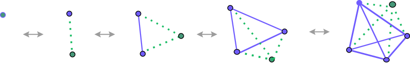
Fig. 1: The D-particle coordinates and the open strings mediating them are denoted by blobs and lines connecting them, respectively. The real lines are open-string degrees of freedom which have been created before the latest operation of the creation field operator, while the dotted lines indicate those created by the last operation. The arrows indicate the operation of creation (from left to right) and annihilation (from right to left) of D-particles.

As we explain below, the multiplication rules of the D-particle field operators are actually not associative, nor commutative, and hence we need some special notation for expressing $N$-body states with $N\geq 3$. But for the moment, let us avoid such complications for the purpose of explaining only the key ideas in the case of simple 1-body and 2-body states.

2.2 Projection condition and the creation operator

The conditions on the effective coordinate degrees of freedom are assumed to be the following recursive requirements:

$$\partial_{y_{1}^{(1)}}\phi^{+}[z^{(1)},\bar{z}^{(1)}]|0\rangle=0,\quad\partial_{z^{(1)}_{k}}\phi^{+}[z^{(1)},\bar{z}^{(1)}]|0\rangle=\partial_{\bar{z}^{(1)}_{k}}\phi^{+}[z^{(1)},\bar{z}^{(1)}]|0\rangle=0\quad\mbox{for}\,\quad k\geq 2,$$

$$\partial_{y_{2}^{(2)}}\phi^{+}[z^{(2)},\bar{z}^{(2)}]\phi^{+}[z^{(1)},\bar{z}^{(1)}]|0\rangle=0,\quad\partial_{z^{(2)}_{k}}\phi^{+}[z^{(2)},\bar{z}^{(2)}]\phi^{+}[z^{(1)},\overline{z}^{(1)}]|0\rangle$$

$$=\partial_{\bar{z}^{(2)}_{k}}\phi^{+}[z^{(2)},\bar{z}^{(2)}]\phi^{+}[z^{(1)},\overline{z}^{(1)}]|0\rangle=0\quad\mbox{for}\,\quad k\geq 3,\quad\mbox{etc.}$$ (2.6)

They require that the non-vanishing results of the creation operator sending a $N$-body state to a $N+1$-body state have nontrivial coordinate dependence only for finite-dimensional sub-manifolds, as we have defined in the previous subsection, and have only zero-mode (in the sense of the conjugate momentum space) dependencies on other components $y_{N}^{(N)}$ and $z^{(N)}_{k}$ with $k\geq N+1$.

To express these conditions concisely for the general case, it is convenient to introduce new notation. Let $P_{1}$ denote the operation of projection which reduces a generic complex vector $(w_{1},w_{2},w_{3},\dots)$ to $(r_{1},0,0,\ldots)$ with $w_{n}=r_{n}+is_{n}$,

$$P_{1}:\,\,(w_{1},w_{2},w_{3},\ldots)\rightarrow(r_{1},0,0,\ldots),$$ (2.7)

and more generally as

$$P_{n}:\,\,(w_{1},w_{2},\ldots,w_{n-1},w_{n},w_{n+1},\ldots)\rightarrow(w_{1},w_{2},\ldots,w_{n-1},r_{n},0,0,0,\ldots),$$ (2.8)

satisfying $P_{n}P_{m}=P_{m}P_{n}=P_{m}$ for $n\geq m.$ Equivalently, we can express the latter conditions as

$$Q_{n}Q_{m}=\delta_{nm}Q_{n},$$ (2.9)

defining $Q_{n}=P_{n}-P_{n-1}$ for $n\geq 2$, and $Q_{1}=P_{1}.$ We use this notation with the following convention: For an arbitrary function $f[w,\bar{w}]$ of complex vectors, the projected functions are defined either as

$$w_{k}f[P_{n},\overline{P_{n}w}]=0\quad\mbox{for}\quad k>n,\quad s_{n}f[P_{n}w,\overline{P_{n}w}]=0$$ (2.10)

or as

$$\partial_{w_{k}}f[\tilde{P}_{n},\overline{\tilde{P}_{n}w}]=0\quad\mbox{for}\quad k>n,\quad\partial_{s_{n}}f[\tilde{P}_{n}w,\overline{\tilde{P}_{n}w}]=0.$$ (2.11)

For brevity, we have denoted the results of projection with respect to the conjugate momentum $p_{n}$ as defined in (2.8) by $\tilde{P}_{n}z$. When we consider the projection in the coordinate representation, we simply write it as $P_{n}z$ without the tilde. This is also the case for our annihilation operator $\phi^{-}$, to be defined later. It should be kept in mind that for non-dummy components, there is clearly no distinction between projection operators with or without the tilde in the base space.

The conditions (2.6) for the creation field acting sequentially upon the vacuum can be expressed by introducing an infinite set of projection operators ${\cal P}_{n}$ $(n=1,2,\ldots)$ in the D-particle Fock space satisfying

$$\phi^{+}[z,\bar{z}]{\cal P}_{n}={\cal P}_{n+1}\phi^{+}[\tilde{P}_{n}z,\tilde{P}_{n}\bar{z}].$$ (2.12)

Unlike the projections $P_{n}$ and $\tilde{P}_{n}$ in the base space, the Fock-space projectors ${\cal P}_{n}$ with different $n$ are assumed to be orthogonal:

$${\cal P}_{n}{\cal P}_{m}=\delta_{mn}{\cal P}_{n}.$$ (2.13)

This is consistent with the orthogonality of the Fock space states with different D-particle numbers. The action of the projection operator ${\cal P}_{n}$ on the creation D-field $\phi^{+}$ makes the projection in the base space of the arguments of the field operators with respect to its momentum space, as manifest in (2.6). The vacuum is assumed to be invariant under the projection ${\cal P}_{1}$ but annihilated by ${\cal P}_{n}$ with $n\geq 2$:

$${\cal P}_{1}|0\rangle=|0\rangle,\quad{\cal P}_{2}|0\rangle={\cal P}_{3}|0\rangle=\cdots=0.$$ (2.14)

Then, the projection conditions (2.6) are succinctly summarized as

$$\phi^{+}[z^{(2)},\bar{z}^{(2)}]\phi^{+}[z^{(1)},\bar{z}^{(1)}]|0\rangle={\cal P}_{3}\phi^{+}[\tilde{P}_{2}z^{(2)},\tilde{P}_{2}\bar{z}^{(2)}]\phi^{+}[\tilde{P}_{1}z^{(1)},\tilde{P}_{1}\bar{z}^{(1)}]|0\rangle.$$ (2.15)

Extension to general $N$-body states is obvious. When we introduce the dual Fock space below, the dual vacuum $\langle 0|$ is assumed to satisfy the same conditions as (2.14),

$$\langle 0|{\cal P}_{1}=\langle 0|,\quad\langle 0|{\cal P}_{2}=\langle 0|{\cal P}_{3}=\cdots=0.$$ (2.16)

These projection conditions should be regarded as the quantum analog of the projector property realized by the lump solutions which are believed to represent D-branes in the vacuum string field theory. As is well known, such a feature has previously been observed in the case of non-commutative solitons [14]. In these cases, the projector property is exhibited by the classical solutions themselves. Such classical solutions must be related to the collective coordinates for solitons, which should constitute the base space for soliton-field operators in a full-fledged quantum theory.

Because of these conditions, it is often convenient and most economical to write these multi-D-particle states by indicating only the components of the coordinates on which the field operators have nontrivial dependencies and suppressing the dummy components, as

$${\cal P}_{2}\phi^{+}[X_{11}]|0\rangle,\quad{\cal P}_{3}\phi^{+}[X_{12},X_{21},X_{22}]\phi^{+}[X_{11}]|0\rangle,\quad\mbox{etc.}$$

2.3 Gauge-statistics conditions and the annihilation operator

We can now impose conditions to account for the second new feature of our D-particle Fock space. The feature 2 of the D-particle Fock space mentioned in the subsection 2.1, is trivial for a 1-body state, being effective only for states with $N\geq 2$. We demand for $N=2$ that

$${\cal P}_{3}\phi^{+}[X_{12},X_{21},X_{22}]\phi^{+}[X_{11}]|0\rangle={\cal P}_{3}\phi^{+}[X^{U(2)}_{12},X^{U(2)}_{21},X^{U(2)}_{22}]\phi^{+}[X^{U(2)}_{11}]|0\rangle,$$ (2.17)

with obvious extension for $N\geq 3$, where

$$X^{U(N)}\equiv U(N)XU(N)^{-1}.$$ (2.18)

Here $U(N)$ is an arbitrary unitary $N\times N$ matrix. This realizes a natural generalization of the condition (2.2) to the present continuous statistical symmetry through the replacement of the permutation symmetry $\{P\}$ by the continuous group U($N$). Although we are forced to abandon the simple commutativity of the creation operators corresponding to the usual Bose-Einstein statistics, we impose instead an extremely strong gauge-symmetry constraint. Compared to ordinary particles, D particles are not only indistinguishable from each other in a stringent sense, but also they are mutually permeable, or, osmotic. We call this new quantum statistics ‘permeable statistics’.

If we use the notation of the projection operators introduced above, we can express the non-dummy components of complex vector coordinates by making the replacement

$$P_{n}z^{(n)}\rightarrow P_{n}XQ_{n},\quad P_{n}\bar{z}^{(n)}\rightarrow Q_{n}XP_{n},$$ (2.19)

using an abstract matrix notation for the right-hand side, which should be understood as

$$(k|P_{n}XQ_{n}|\ell)=\delta_{\ell n}X_{k\ell}\quad\mbox{for}\quad k\leq n,$$ (2.20)

$$(\ell|Q_{n}XP_{n}|k)=\delta_{\ell n}X_{\ell k}\quad\mbox{for}\quad k\leq n,$$ (2.21)

or as

$$Q_{n}|k)=\delta_{nk}|k),\quad(k|Q_{n}=\delta_{nk}(k|.$$ (2.22)

Here, the variable $X$ is a generic infinite-dimensional operator whose projection is assumed to be the corresponding finite-dimensional matrix variable. In terms of this notation, the transformation (2.18) is nothing but the change of basis

$$|n)\rightarrow|n)^{\prime}=\sum_{m=1}^{N}U(N)^{-1}_{mn}|m)\quad(n|\rightarrow(n|^{\prime}=\sum_{m=1}^{N}U(N)_{nm}(m|$$ (2.23)

for $n\leq N$, under which $P_{N}$ is invariant

$$P_{N}=\sum_{n=1}^{N}|n)(n|=\sum_{n=1}^{N}|n)^{\prime}(n|^{\prime}.$$ (2.24)

Thus, the gauge-statistics condition requires that the $N$-body states be invariant under the change of the maximal set $\{|1),|2),\ldots,|N)\}$ of the basis for the $N\times N$ matrices of the $N$-body states.

Our next task is to define the annihilation operator $\phi^{-}[z,\bar{z}]$ for D particles. Its action must be consistent with the above properties of the creation operator. First, for the vacuum, we have

$$\phi^{-}[z,\overline{z}]|0\rangle=0.$$ (2.25)

Then, for 1-body state, we define

$$\phi^{-}[z,\overline{z}]\phi^{+}[z^{(1)},\overline{z}^{(1)}]|0\rangle=\delta(x_{1}-x^{(1)}_{1})\delta(y_{1})\prod_{k\geq 2}\delta^{2}(z_{k})|0\rangle,$$ (2.26)

where $\delta^{2}(z)=\delta(z)\delta(\bar{z})$. We use the following abbreviation for the product of an infinite number of $\delta$-functions:

$$\sigma_{\ell}\equiv\delta(y_{\ell})\prod_{k>\ell}\delta^{2}(z_{k}).$$ (2.27)

Note that here and in what follows, we suppress the dimension parameter $d$ on the $\delta$-functions for spatial vectors. Thus, we write $\delta(y)=\delta^{d}(y),\delta^{2}(z)=\delta^{2d}(z)$, etc.

The attentive reader might wonder why we here use the position space $\delta$-functions for the dummy components of $(z,\bar{z})$, in spite of the fact that the projection of the dummy components for the creation fields is done in the momentum space. The reason is that for the annihilation field, we assume the projection to take the following form

$${\cal P}_{n}\phi^{-}[P_{n}z,P_{n}\bar{z}]=\phi^{-}[z,\bar{z}]{\cal P}_{n+1},$$ (2.28)

where the projections $P_{n}z$ with respect to the basis space of the complex vectors are effective in the coordinate representation, in contrast to the creation field. Such mutually conjugate projections of dummy components for the creation and annihilation operators are necessary in order to ensure the reduction of the number of degrees of freedom in a well-defined way for $N$-body D-particle states from infinite dimensions. By so doing, the parts of the Hamiltonian and other observables become null for the dummy variables as desired. Otherwise we would encounter various annoying infinities in making the reductions. We do not claim uniqueness for our construction: For example, in our present formulation in flat space, the theory is invariant under $(z^{i}_{n},\bar{z}_{n}^{i})\rightarrow(z^{i}_{n},\bar{z}_{n}^{i})+(c^{i},c^{i})$, as we show below. Thus we can at least shift the origin of the infinite-dimensional vector space accordingly.

Beyond the above remarks on the projection condition, the two properties of the annihilation operator stated above need no further explanation. A non-trivial feature appears from 2-body states. As a natural extension of (2.3), we define the action of the annihilation field to the 2-body state by

$$\phi^{-}[z,\overline{z}]\phi^{+}[z^{(2)},\bar{z}^{(2)}]\phi^{+}[z^{(1)},\bar{z}^{(1)}]|0\rangle=\phi^{-}[z,\overline{z}]{\cal P}_{3}\phi^{+}[X_{12},X_{21},X_{22}]\phi^{+}[X_{11}]|0\rangle$$

$$={\cal P}_{2}\int[dU(2)]\delta(x_{2}-X^{U(2)}_{22})\delta^{2}(z_{1}-X^{U(2)}_{12})\sigma_{2}\phi^{+}[X^{U(2)}_{11}]|0\rangle.$$ (2.29)

Here, the group integration measure $[dU(N)]$ is normalized as

$$\int[dU(N)]=N.$$ (2.30)

An important characteristic of this definition is that we introduced the integration $[dU(N)]$ over the $U(N)$ $(N=2)$ transformations explicitly in order to preserve the gauge-statistics condition of the original state, $\phi^{+}[z^{(2)},\bar{z}^{(2)}]\phi^{+}[z^{(1)},\bar{z}^{(1)}]|0\rangle$, before acting with the annihilation field. This, of course, corresponds to the summation $\sum_{P}$ over different permutations $\{P\}$ in (2.3) of the $N$-body states of ordinary particles, and it replaces the role of the canonical commutator $[\psi(x),\psi^{\dagger}(y)]=\delta(x-y)$ between annihilation and creation fields for ordinary particles.

2.4 Non-associativity

Before going on to formulate the properties for D-particle fields for the general $N$-body state, it is appropriate here to give further analysis concerning the nature of the decomposition of matrix variables into sets of infinite-dimensional complex vectors. Due to the existence of the off-diagonal components of matrix variables, we cannot, generically, reduce the action of a subgroup of a gauge transformation group to a smaller subset of variables of matrix components. In contrast to this, in the case of the permutation group, any permutation within a subset of particles does not affect the remaining particle degrees of freedom. This implies that, when we consider a mapping from $N$-body to $(N+1)$-body states of D particles, the gauge-statistics condition of the former cannot be embedded into the latter without affecting the new degrees of freedom added by the operation of creating a D-particle.

For example, suppose that a gauge transformed $N\times N$ matrix $X^{U(N)}=U(N)XU(N)^{-1}$ of an $N$-body state is embedded naturally in an $(N+1)\times(N+1)$ matrix of an $(N+1)$-body state as

$$X^{\hat{U}(N)}\equiv\begin{pmatrix}X^{U(N)}_{1,1}&X^{U(N)}_{1,2}&\cdots&X^{U(N)}_{1,N}&X_{1,N+1}\cr X^{U(N)}_{2,1}&X^{U(N)}_{2,2}&\cdots&X^{U(N)}_{2,N}&X_{2,N+1}\cr\cdot&\cdot&\cdot&\cdot&\cdot\cr\cdot&\cdot&\cdot&\cdot&\cdot\cr\cdot&\cdot&\cdot&\cdot&\cdot\cr X^{U(N)}_{N,1}&X^{U(N)}_{N,2}&\cdots&X^{U(N)}_{N,N}&X_{N,N+1}\cr X_{N+1,1}&X_{N+1,2}&\cdots&X_{N+1,N}&X_{N+1,N+1}\end{pmatrix}.$$

But this is different from the $(N+1)\times(N+1)$ matrix

$$X^{U(N+1;N)},$$

which is obtained with the $(N+1)\times(N+1)$ unitary transformation containing the $N\times N$ transformation $U(N)$ as a block-diagonal matrix as

$$U(N+1;N)\equiv\begin{pmatrix}U(N)&0\cr 0&1\cr\end{pmatrix}.$$ (2.31)

In the latter case, the $N$-th column and row must be replaced, respectively, by $(a,b\leq N)$

$$z^{(N+1)}_{a}=X_{a,N+1}\rightarrow U(N)_{ab}X_{b,N+1},\quad\bar{z}^{(N+1)}_{a}=X_{N+1,a}\rightarrow X_{N+1,b}U(N)^{-1}_{ba},$$ (2.32)

compared with $X^{\hat{U}(N)}$ in the above expression. Thus, a U($N$) adjoint transformation of the $N\times N$ sub-matrix must necessarily be associated with a U($N$) transformation of the added column and row of the $(N+1)\times(N+1)$ matrix in which the original $N\times N$ matrix is embedded.

This means that an $N$-ple product of the D-particle creation fields cannot be decomposed into a form which is composed of products with smaller numbers of them for states with smaller $N$. Thus, the algebra of D-particle creation operators are, so to speak, maximally non-associative. In order to express this situation explicitly, we denote the $N$-body state created by the product of $N$ creation fields in the form

$$|N[X]\rangle\equiv{\cal P}_{N}[[\phi^{+}[X_{N}]\phi^{+}[X_{N-1}]\cdots\phi^{+}[X_{1}]]]|0\rangle,$$ (2.33)

employing a special delimiter symbol $[[***]]$ for the ordered products ($***$) of field operators. By definition, the state (2.33) satisfies the gauge-statistics condition

$$[[\phi^{+}[X_{N}]\phi^{+}[X_{N-1}]\cdots\phi^{+}[X_{1}]]]|0\rangle=[[\phi^{+}[X^{U(N)}_{N}]\phi^{+}[X^{U(N)}_{N-1}]\cdots\phi^{+}[X^{U(N)}_{1}]]]|0\rangle.$$ (2.34)

Note that here (and mostly in what follows) we use abbreviated notation for matrix variables as the arguments for the field operators: The complex vectors for which each creation field has nontrivial dependence are denoted by $(z^{(n)},\bar{z}^{(n)})\rightarrow X_{n}$, with $n=1,2,\ldots,N$ for the $N$-body state. Thus, for example, $X_{N}$ collectively represents the set of $2N+1$ elements given by

$$(X_{1,N},X_{N,1},X_{2,N},X_{N,2},\ldots,X_{N-1,N},X_{N,N-1},X_{N,N}).$$

At this juncture, we add one side remark concerning the decomposability of the multiplication rule for creation operators. Consider a U($N$) matrix of the form

$$U(N;n)\equiv\begin{pmatrix}1_{N-n}&0\cr 0&U(n)\cr\end{pmatrix},$$

with $U(n)$ being an $n\times n$ unitary matrix. The adjoint action of this matrix on an $N$-body matrix variables by this matrix affects its columns and rows corresponding only to the $n$-th, $(n+1)$-th, $\ldots$, $N$-th creation fields, i.e. $\phi^{+}[X_{n}],\ldots,\phi^{+}[X_{N}]$. This suggests the possibility of nesting the non-associative $N$-ple multiplication of the creation operators into a particular set of successive multiplications from the left to the right as

$$[[\phi^{+}[X_{N}]\phi^{+}[X_{N-1}]\cdots\phi^{+}[X_{1}]]]|0\rangle\sim((\cdots((\phi^{+}[X_{N}]\phi^{+}[X_{N-1}])\phi^{+}[X_{N-2}])\cdots)\phi^{+}[X_{1}])|0\rangle.$$

This is not suitable for studying recursive multiplications of field operators from right to left, corresponding to the creation of D-particles one by one, yielding states with increasing number particle number. But it is certainly suggestive of a certain algebraic characterization of the D-particle field operators. We leave further investigation of this and related aspects of D-particle fields for future works.

2.5 Two classes of operations in the Fock space

With the above feature in mind, the operation $|N[X]\rangle\xrightarrow{\phi^{+}[z]}|(N+1)[X]\rangle$ that sends the $N$-body state $|N[X]\rangle$ to the $N+1$-body state by inserting a new creation field $\phi^{+}[X_{N+1}]$ into the bracket symbol $[[***]]$,

$$|(N+1)[X]\rangle={\cal P}_{N+2}[[\phi^{+}[X_{N+1}]\phi^{+}[X_{N}]\phi^{+}[X_{N-1}]\cdots\phi^{+}[X_{1}]]]|0\rangle,$$ (2.35)

is represented by the new symbol $\triangleright[[\,\,=\triangleright[[\hskip 3.0pt$ as

$$\phi^{+}[z](|N[X]\rangle)\equiv\phi^{+}[z]\triangleright|N[X]\rangle$$

$$={\cal P}_{N+2}\phi^{+}[X_{N+1}]\triangleright[[\hskip 4.0pt\phi^{+}[X_{N}]\phi^{+}[X_{N-1}]\cdots\phi^{+}[X_{1}]]]|0\rangle$$

$$={\cal P}_{N+2}[[\phi^{+}[X_{N+1}]\phi^{+}[X_{N}]\phi^{+}[X_{N-1}]\cdots\phi^{+}[X_{1}]]]|0\rangle.$$ (2.36)

Thus, this new symbol represents the operation of adding a new blob and off-diagonals, depicted by the dotted lines in Fig. 1. If this process is formally interpreted as the multiplication of the bracket $[[***]]$ by creation fields from the left, it is not invariant under the $U(N)$ transformation in the sense of the original $N$-body state,

$$\phi^{+}[X_{N+1}]\triangleright[[\hskip 4.0pt\phi^{+}[X^{U(N)}_{N}]\phi^{+}[X^{U(N)}_{N-1}]\cdots\phi^{+}[X^{U(N)}_{1}]]]|0\rangle$$

$$\neq\phi^{+}[X_{N+1}]\triangleright[[\hskip 4.0pt\phi^{+}[X_{N}]\phi^{+}[X_{N-1}]\cdots\phi^{+}[X_{1}]]]|0\rangle,$$

but instead satisfies the $N+1$-body gauge-statistics condition, of which a special case is

$$|(N+1)[X^{\hat{U}(N)}]\rangle={\cal P}_{N+2}\phi^{+}[X_{N+1}]\triangleright[[\hskip 4.0pt\phi^{+}[X^{U(N)}_{N}]\phi^{+}[X^{U(N)}_{N-1}]\cdots\phi^{+}[X^{U(N)}_{1}]]]|0\rangle$$

$$={\cal P}_{N+2}\phi^{+}[X^{U(N+1;N)}_{N+1}]\triangleright[[\hskip 4.0pt\phi^{+}[X_{N}]\phi^{+}[X_{N-1}]\cdots\phi^{+}[X_{1}]]]|0\rangle$$ (2.37)

$$={\cal P}_{N+2}[[\phi^{+}[X^{U(N+1;N)}_{N+1}]\phi^{+}[X_{N}]\phi^{+}[X_{N-1}]\cdots\phi^{+}[X_{1}]]]|0\rangle,$$

where $X^{U(N+1;N)}_{N+1}$ indicates the replacement given in (2.32).

This peculiarity does not create any immediate inconsistency if we forbid this operation from appearing in physical processes, even though care must be taken in treating these operators. This signifies that our D-particle fields themselves should not be regarded directly as physical observables. There is a similar situation in ordinary field theory; recall that any non-singlet fields in general gauge field theories cannot be regarded directly as gauge-invariant observables, but are still useful as intermediate tools for constructing observables. As a matter of fact, the creation of a D particle not accompanied by the simultaneous creation of an anti-D-particle is forbidden, due to the RR-charge conservation from the bulk viewpoint also.

It is convenient to classify various operations in our D-particle Fock space according to the following criterion. If an operation ${\cal O}$ acting on an $N$-body state preserves the gauge-statistics condition, i.e.

$${\cal O}|N[X]\rangle={\cal O}|N[X^{U(N)}]\rangle,$$ (2.38)

the operation ${\cal O}$ is defined to be A-class. Otherwise, it will be called B-class. Thus the D-particle creation field acting to the right is B-class. However, it is possible that a B-class operation can become A-class when it is combined with other operations. In general, any operator representing observables must be A-class, though the converse need not be true, depending on further criteria for ‘physical’ operations. We see below that integrated local bilinear forms of the creation and annihilation fields are A-class in general, and they obey the ordinary algebra of gauge-invariants when acting upon states.

Let us now fix the definition of the annihilation operator by extending that given above for the 2-body case to general $N$-body states. Using the new symbols, the action of the annihilation field for a general $N$-body state is expressed as

$$\phi^{-}[z,\overline{z}]|N[X]\rangle=\phi^{-}[z,\overline{z}]{\cal P}_{N+1}[[\phi^{+}[X_{N}]\phi^{+}[X_{N-1}]\cdots\phi^{+}[X_{1}]]]|0\rangle$$

$$=\phi^{-}[z,\bar{z}]{\cal P}_{N+1}\phi^{+}[X_{N}]\triangleright[[\hskip 4.0pt\phi^{+}[X_{N-1}]\phi^{+}[X_{N-2}]\cdots\phi^{+}[X_{1}]]]|0\rangle$$

$$=\int[dV(N)]\,\delta(x_{N}-X^{V(N)}_{NN})\delta^{2}(z_{1}-X^{V(N)}_{1N})\delta^{2}(z_{2}-X^{V(N)}_{2N})\cdots\delta^{2}(z_{N-1}-X^{V(N)}_{N-1,N})\sigma_{N}$$

$$\times\,{\cal P}_{N}[[\phi^{+}[X^{V(N)}_{N-1}]\phi^{+}[X^{V(N)}_{N-2}]\cdots\phi^{+}[X_{1}^{V(N)}]]]|0\rangle.$$ (2.39)

Note that the delimiter in the first line is still “$[[$”, corresponding to the fact that the operation of annihilation applied to ket-states preserves the gauge statistics condition of the $N$-body states, owing to the U($N$)-integration, and hence it is A-class when acting to the right.

2.6 Dual states

Using a general gauge invariant wave function $\Psi[X]=\Psi[X^{U(N)}]$ in the configuration space, a general $N$-body state vector in the Fock space takes the form

$$|\Psi\rangle=\int\frac{[d^{d}X]}{[dU(N)]}\Psi[X]|N[X]\rangle,$$ (2.40)

where in the integration over the matrix coordinates, the gauge redundancy is completely removed by the denominator representing the gauge volume, $[dU(N)]$. To complete the formalism, it is necessary to define dual states that are conjugate to these ket-states. The bra-vacuum satisfies

$$\langle 0|\phi^{+}[z,\bar{z}]=0,\quad\langle 0|0\rangle=1,$$

with the projection condition (2.16). Then the general dual $N$-body states are given by

$$\langle\Psi|=\int[d^{2d}\hat{z}]_{N}\int\frac{[d^{d}Y]}{[dU[N]]}\overline{\Psi[Y]}\langle N[Y;\hat{z}]|{\cal P}_{N}$$ (2.41)

in terms of the dual $N$-body basis state

$$\langle N[Y;\hat{z}]|=\langle 0|[[\phi^{-}[Y_{1};\hat{z}^{(1)}]\phi^{-}[Y_{2};\hat{z}^{(2)}]\cdots\phi^{-}[Y_{N};\hat{z}^{(N)}]]],$$ (2.42)

where we have denoted the components with nontrivial dependencies by $Y_{n}$. The symbols $\hat{z}^{(n)}$ collectively represent the remaining dummy components of the complex vector coordinates

$$\hat{z}^{n}:\,\{y^{(n)}_{n};z^{(n)}_{n+1},z^{(n)}_{n+2},\ldots,;\bar{z}^{(n)}_{n+1},\bar{z}^{(n)}_{n+2},\ldots\},$$

with respect to which the state vector has only $\delta$-function supports at zero, by the definition of the action of the annihilation fields, owing to the projection condition (2.28). Correspondingly, the symbol $[d^{2d}\hat{z}]_{N}$ in (2.41) indicates integrations over them. However, it should be recalled that the wave function $\overline{\Psi[X]}$ is simply the complex conjugate of the Yang-Mills wave function $\Psi[X]$, which is independent of the dummy components. Therefore, when the dual bra-states are coupled with the ket-states, the integration $\int[d^{2d}\hat{z}]_{N}$ over these remaining components simply gives 1. Hence, we can in practice suppress these variables for notational brevity, as we do in what follows, unless otherwise specified.

Using a similar convention similar to that used in the case of the ket-states, we define the new right delimiter symbol $]]\triangleright=\,\triangleright]]\,$ and denote the operation to the left sending the dual $(N-1)$-body basis vector to the $N$-body basis vector as

$$\langle N[Y;\hat{z}]|=\langle 0|[[\phi^{-}[Y_{1};\hat{z}^{(1)}]\phi^{-}[Y_{2};\hat{z}^{(2)}]\cdots\phi^{-}[Y_{N-1};\hat{z}^{(N-1)}]\,\triangleright]]\,\phi^{-}[Y_{N};\hat{z}^{(N)}],$$ (2.43)

or, by suppressing the dummy variables, simply as

$$\langle N[Y]|=\langle 0|[[\phi^{-}[Y_{1}]\phi^{-}[Y_{2}]\cdots\phi^{-}[Y_{N-1}]\,\triangleright]]\,\phi^{-}[Y_{N}]$$

$$=\langle 0|[[\phi^{-}[Y_{1}]\phi^{-}[Y_{2}]\cdots\phi^{-}[Y_{N-1}]\phi^{-}[Y_{N}]]]$$

using the same convention as for the ket-states. The scalar product of two states can be computed using our rules. It is evident that they are non-vanishing only for states with the same numbers of D particles. For 1-body states, we obviously have

$$\langle\Psi^{\prime}|\Psi\rangle=\int d^{d}Y_{11}\int d^{d}X_{11}\overline{\Psi^{\prime}[Y]}\Psi[X]\delta(Y_{11}-X_{11}).$$

For general $N$-body states, we have

$$\langle\Psi^{\prime}|\Psi\rangle=N!\int\frac{[d^{d}Y]}{[dU(N)]}\int\frac{[d^{d}X]}{[dU(N)]}\overline{\Psi^{\prime}[Y]}\Psi[X]\delta[Y-X].$$ (2.44)

The $\delta$-function for the matrices $\delta[Y-X]$ is an $dN^{2}$-dimensional $\delta$-function with respect to the $dN^{2}$ integration measure for the matrix coordinates, equating all the $dN^{2}$ real components of two $d$-dimensional $N\times N$ hermitian matrices $X$ and $Y$.

Indeed, after integration over the dummy vector components, which simply gives 1, we have

$$\int\frac{[d^{d}Y(N)]}{[dU(N)]}\int\frac{[d^{d}X(N)]}{[dU(N)]}\,\overline{\Psi^{\prime}[Y]}\Psi[X]\langle N[Y]|N[X]\rangle=$$

$$\int\frac{[d^{d}Y(N)]}{[dU(N)]}\int\frac{[d^{d}X(N)]}{[dU(N)]}\,\overline{\Psi^{\prime}[Y]}\Psi[X]$$

$$\times\langle 0|[[\phi^{-}[Y_{1}]\phi^{-}[Y_{2}]\cdots\phi^{-}[Y_{N-1}]\,\triangleright]]\,\phi^{-}[Y_{N}]\phi^{+}[X_{N}]\triangleright[[\hskip 4.0pt\phi^{+}[X_{N-1}]\phi^{+}[X_{N-2}]\cdots\phi^{+}[X_{1}]]]|0\rangle$$

$$=\int\frac{[d^{d}Y(N)]}{[dU(N)]}\int\frac{[d^{d}X(N)]}{[dU(N)]}\,\overline{\Psi^{\prime}[Y]}\Psi[X]\int[dV(N)]\langle(N-1)[Y]|(N-1)[X_{N}^{V(N)}]\rangle\delta[Y_{N}-X_{N}^{V(N)}]$$

$$=\int\frac{[d^{d}Y(N)]}{[dU(N)]}\int\frac{[d^{d}X(N)]}{[dU(N)]}\,\overline{\Psi^{\prime}[Y]}\Psi[X]\int[dV(N)]\langle(N-1)[Y]|(N-1)[X]\rangle\delta[Y_{N}-X_{N}]$$

$$=N\int\frac{[d^{d}Y(N)]}{[dU(N)]}\int\frac{[d^{d}X(N)]}{[dU(N)]}\,\overline{\Psi^{\prime}[Y]}\Psi[X]\langle(N-1)[Y]|(N-1)[X]\rangle\delta[Y_{N}-X_{N}].$$

Note that here the $\delta$-function $\delta[Y_{N}-X_{N}]$ is one of $d(2(N-1)+1)$ dimensions. This leads to the above conclusion, (2.44), utilizing the fact that the wave functions $\Psi[X]$ and $\Psi^{\prime}[Y]$ and the states $|n[X]\rangle$ and $\langle n[Y]|$ $(n=1,2,\ldots,N)$ are all independently invariant under gauge transformations. It is also to be noted that the $\delta$-functions $\delta[Y_{n}-X_{n}]$ can be replaced by $\delta[Y_{m}^{U(N,n)}-X_{m}^{U(N,n)}]$ $(m\geq n)$ in the case that we embed an arbitrary U($n$) matrix into U($N$), as in the definition (2.31) with $n=N-1$ and its obvious generalization to general $n\,(<N)$. This is necessary to reduce the last line to lower body states recursively. We have thus seen that our Fock space admits the ordinary probability interpretation, even though we have to deal with the non-associative rule for the multiplication of field operators.

The above property of the dual states also allows us to assume the action of the creation operator to bra-states from the right to the left in the following form :

$$\langle N[Y]|\phi^{+}[z,\bar{z}]=\langle 0|[[\phi^{-}[Y_{1}]\phi^{-}[Y_{2}]\cdots\phi^{-}[Y_{N-1}]\phi^{-}[Y_{N}]]]\phi^{+}[z,\bar{z}]{\cal P}_{N-1}$$

$$=\langle 0|[[\phi^{-}[Y_{1}]\phi^{-}[Y_{2}]\cdots\phi^{-}[Y_{N-1}]\,\triangleright]]\,\phi^{-}[Y_{N}]\phi^{+}[z,\bar{z}]{\cal P}_{N-1}$$

$$=\int[dV(N)]\delta(x_{N}-Y^{V(N)}_{NN})\delta^{2}(z_{1}-Y_{1N}^{V(N)})\delta^{2}(z_{2}-Y_{2N}^{V(N)})\cdots\delta^{2}(z_{N-1}-Y_{N-1,N}^{V(N)})$$

$$\times\langle 0|[[\phi^{-}[Y^{V(N)}_{1}]\phi^{-}[Y^{V(N)}_{2}]\cdots\phi^{-}[Y^{V(N)}_{N-1}]]].$$ (2.45)

It is to be noted that this expression is independent of $y_{N}$ and of $z_{n}$ and $\bar{z}_{n}$ with $n>N$, in accordance with the projection condition (2.12) satisfied by the creation operator $\phi^{+}[z,\bar{z}]$.

These results show that the classification of operators defined in the previous subsection actually depends on the directions of the operations: The creation operator is B-class when acting from the left to the right, but A-class when acting from the right to the left. Conversely, the annihilation operator is A-class from the left to the right and B-class from the right to the left. In this way, the apparent asymmetry between the creation and annihilation operators is resolved by taking into account the dual Fock space. Operators corresponding to physical processes must be A-class in both directions.

3. Bilinears as physical operators

We are now ready to discuss how to express ordinary gauge-invariant physical observables including the Hamiltonian in terms of our D-particle field operators. As in the ordinary second quantization, they are essentially given by bilinear forms of D-particle field operators,

$$\langle\phi^{+},F\phi^{-}\rangle\equiv\int[d^{2d}z]\,\phi^{+}[z,\bar{z}]\triangleright F\phi^{-}[z,\bar{z}].$$ (3.1)

We include the symbol $\triangleright$ here to explicitly indicate that we are using the rule of multiplication of the creation operator $\phi^{+}$ to the right and of the annihilation operator $\phi^{-}$ to the left, simultaneously, following the discussion in the previous section. The symbol $F$ can in general represent operators with respect to the vector coordinates $(z,\bar{z})$. Obviously, these bilinear forms commutes with the projection conditions, i.e.

$$[{\cal P}_{n},\langle\phi^{+},F\phi^{-}\rangle]=0,$$ (3.2)

and also are A-class in both directions of their operation. Since their properties when acting on states are essentially symmetric with respect to ket-states and bra-states, it is sufficient to study their actions on ket-states.

3.1 Bilinear operators without derivatives

Let us first consider the case $F=F[z,\bar{z}]$, which does not involve differential operators in $z$ and $\bar{z}$. By studying the action of this bilinear form on a general $N$-body ket-state $|N[X]\rangle$, we find

$$\int[d^{2d}z]\,\phi^{+}[z,\bar{z}]\triangleright F\phi^{-}[z,\bar{z}]|N[X]\rangle$$

$$=\int[d^{2d}z]F[z,\bar{z}]\int[dU(N)]\,\delta(x_{N}-X^{U(N)}_{NN})\delta^{2}(z_{1}-X^{U(N)}_{1N})\delta^{2}(z_{2}-X^{U(N)}_{2N})\cdots\delta^{2}(z_{N-1}-X^{U(N)}_{N-1,N})\sigma_{N}$$

$$\times\,\phi^{+}[z,\bar{z}]{\cal P}_{N-1}\triangleright[[\hskip 4.0pt\phi^{+}[X^{U(N)}_{1,N-1},X^{U(N)}_{2,N-1},\ldots,\bar{X}^{U(N)}_{1,N-1},\bar{X}^{U(N)}_{2,N-1},\ldots,X_{N-1,N-1}^{U(N)}]\cdots\phi^{+}[X_{11}^{U(N)}]]]|0\rangle$$

$$={\cal P}_{N}\int[dU(N)]\,F[X_{1,N}^{U(N)},X_{2,N}^{U(N)},\ldots,\bar{X}_{1,N}^{U(N)},\bar{X}_{2,N}^{U(N)},\ldots,X_{N,N}^{U(N)},0,\ldots]$$

$$\times[[\phi^{+}[X_{1,N}^{U(N)},X_{2,N}^{U(N)},\ldots,\bar{X}_{1,N}^{U(N)},\bar{X}_{2,N}^{U(N)},\ldots,X_{N,N}^{U(N)}]$$

$$\times\phi^{+}[X^{U(N)}_{1,N-1},X^{U(N)}_{2,N-1},\ldots,\bar{X}^{U(N)}_{1,N-1},\bar{X}^{U(N)}_{2,N-1},\ldots,X_{N-1,N-1}^{U(N)}]\cdots\phi^{+}[X_{11}^{U(N)}]]]|0\rangle$$

$$=\int[dU(N)]\,F[X_{1,N}^{U(N)},X_{2,N}^{U(N)},\ldots,\bar{X}_{1,N}^{U(N)},\bar{X}_{2,N}^{U(N)},\ldots,X_{N,N}^{U(N)},0,\ldots]|N[X]\rangle,$$ (3.3)

where in the last equality we have used the gauge-statistical symmetry of the general $N$-body state $|N[X]\rangle=|N[X^{U(N)}]\rangle$.

Examples:

The simplest example is the number operator with $F=1$,

$$\langle\phi^{+},\phi^{-}\rangle|N[X]\rangle=N|N[X]\rangle.$$ (3.4)

The next simplest case, $F_{n}=z^{i}_{n},$ gives

$$\langle\phi^{+},z_{n}\phi^{-}\rangle|N[X]\rangle=\int[dU(N)](U(N)X^{i}U(N)^{-1})_{n,N}|N[X]\rangle={\rm Tr}(X^{i})\delta_{n,N}|N[X]\rangle,$$ (3.5)

using the formula

$$\int[dU(N)]U(N)_{ab}U(N)^{-1}_{cd}=\delta_{ad}\delta_{bc}.$$ (3.6)

Note that for $n>N$, the projection condition for the annihilation operator is responsible for the vanishing result, while for $n<N$, the group integration is. Thus, we have

$$\langle\phi^{+},\sum_{n=1}^{\infty}z_{n}\phi^{-}\rangle|N[X]\rangle={\rm Tr}(X^{i})|N[X]\rangle.$$ (3.7)

Actually, $F=\bar{z}_{n}^{i}$ gives the same expression,

$$\langle\phi^{+},\sum_{n=1}^{\infty}\bar{z}_{n}\phi^{-}\rangle|N[X]\rangle={\rm Tr}(X^{i})|N[X]\rangle.$$ (3.8)

For a quadratic form,

$$F=\sum_{n=1}^{\infty}z^{i}_{n}\bar{z}_{n}^{j}\equiv\bar{z}^{j}\cdot z^{i}$$

which is manifestly invariant under the infinite-dimensional global transformation $z_{n}\rightarrow(Uz)_{n}$, with $U$ being an arbitrary unitary U($\infty$) matrix, we arrive at the integral

$$\int[dU(N)](U(N)X^{j}U(N)^{-1})_{N,n}(U(N)X^{i}U(N)^{-1})_{n,N}$$

$$=\int[dU(N)](U(N)X^{j}X^{i}U(N)^{-1})_{N,N}={\rm Tr}(X^{j}X^{i}),$$

giving

$$\langle\phi^{+},\bar{z}^{j}\cdot z^{i}\phi^{-}\rangle|N[X]\rangle={\rm Tr}(X^{j}X^{i})|N[X]\rangle.$$ (3.9)

An example of 3rd-order invariants is obtained by considering $F_{n}=(\bar{z}^{i}\cdot z^{j})z^{k}_{n}.$ Acting with the corresponding bilinear form on an $N$-body basis state, we have the $U(N)$ integral

$$\int[dU(N)]U(N)_{Na}(X^{i}X^{j})_{ab}U(N)_{bN}^{-1}U(N)_{nc}X_{cd}^{k}U(N)^{-1}_{dN}$$

$$=\int[dU(N)]U(N)_{Na}U(N)_{nc}U(N)_{bN}^{-1}U(N)^{-1}_{dN}(X^{i}X^{j})_{ab}X_{cd}^{k}$$

$$=\Big{(}\frac{N}{N^{2}-1}(\delta_{NN}\delta_{nN}\delta_{ab}\delta_{cd}+\delta_{NN}\delta_{nN}\delta_{ad}\delta_{cb})-\frac{1}{N^{2}-1}(\delta_{NN}\delta_{nN}\delta_{ab}\delta_{cd}+\delta_{NN}\delta_{nN}\delta_{ad}\delta_{cb})\Big{)}$$

$$\times(X^{i}X^{j})_{ab}X_{cd}^{k}$$

$$=\delta_{nN}\frac{1}{N+1}\Big{(}{\rm Tr}(X^{i}X^{j}){\rm Tr}(X^{k})+{\rm Tr}(X^{i}X^{j}X^{k})\Big{)}$$

which gives

$$\delta_{nN}\frac{1}{N+1}{\rm Tr}([X^{i},X^{j}]X^{k})|N[X]\rangle=\langle\phi^{+},(\bar{z}^{i}\cdot z^{j}-\bar{z}^{j}\cdot z^{i})z^{k}_{n}\phi^{-}\rangle|N[X]\rangle.$$ (3.10)

Here use has been made of the integration formula

$$\int[dU(N)]\,U(N)_{a_{1}b_{1}}U(N)_{a_{2}b_{2}}U(N)^{-1}_{c_{1}d_{1}}U(N)^{-1}_{c_{2}d_{2}}$$

$$={N\over N^{2}-1}(\delta_{a_{1}d_{1}}\delta_{a_{2}d_{2}}\delta_{b_{1}c_{1}}\delta_{b_{2}c_{2}}+\delta_{a_{1}d_{2}}\delta_{a_{2}d_{1}}\delta_{b_{1}c_{2}}\delta_{b_{2}c_{1}})$$

$$-{1\over N^{2}-1}(\delta_{a_{1}d_{2}}\delta_{a_{2}d_{1}}\delta_{b_{1}c_{1}}\delta_{b_{2}c_{2}}+\delta_{a_{1}d_{1}}\delta_{a_{2}d_{2}}\delta_{b_{1}c_{2}}\delta_{b_{2}c_{1}}).$$ (3.11)

Thus, for arbitrary $N$, we can use the expression

$$\sum_{n=1}^{\infty}\langle\phi^{+},(\bar{z}^{i}\cdot z^{j}-\bar{z}^{j}\cdot z^{i})z_{n}^{k}\phi^{-}\rangle|N[X]\rangle=\frac{1}{N+1}{\rm Tr}([X^{i},X^{j}]X^{k})|N[X]\rangle$$ (3.12)

similarly to the case of the 1st-order invariant (3.7). This expression is suitable when we consider the so-called Myers term.

As is evident from the derivation, the last expression for odd invariants is not unique. For instance, we can instead consider $F_{n}=(\bar{z}^{i}\cdot z^{j})\bar{z}_{n}^{k}.$ Then, we have the U($N$) integral

$$\int[dU(N)]U(N)_{Na}(X^{i}X^{j})_{ab}U(N)_{bN}^{-1}U(N)_{Nc}X_{cd}^{k}U(N)^{-1}_{dn}$$

$$=\int[dU(N)]U(N)_{Na}U(N)_{Nc}U(N)_{bN}^{-1}U(N)^{-1}_{dn}(X^{i}X^{j})_{ab}X_{cd}^{k}$$

$$=\Big{(}\frac{N}{N^{2}-1}(\delta_{NN}\delta_{nN}\delta_{ab}\delta_{cd}+\delta_{NN}\delta_{nN}\delta_{ad}\delta_{cb})-\frac{1}{N^{2}-1}(\delta_{NN}\delta_{nN}\delta_{ab}\delta_{cd}+\delta_{NN}\delta_{nN}\delta_{ad}\delta_{cb})\Big{)}$$

$$\times(X^{i}X^{j})_{ab}X_{cd}^{k}$$

$$=\delta_{nN}\frac{1}{N+1}\Big{(}{\rm Tr}(X^{i}X^{j}){\rm Tr}(X^{k})+{\rm Tr}(X^{i}X^{j}X^{k})\Big{)}.$$

Thus we have an identity for two odd-degree bilinear operators as the action on states.

$$\langle\phi^{+},(\bar{z}^{i}\cdot z^{j})\bar{z}_{n}^{k}\phi^{-}\rangle=\langle\phi^{+},(\bar{z}^{i}\cdot z^{j})z_{n}^{k}\phi^{-}\rangle.$$ (3.13)

In order to obtain the standard of the Hamiltonian for the low-energy effective D-particle dynamics, it is sufficient to consider terms up to 4-th order in $(z,\bar{z})$, such as $F[z,\bar{z}]=(\bar{z}^{i}\cdot z^{j})(\bar{z}^{i}\cdot z^{j}).$ We find

$$\int[dU(N)]\,U(N)_{Na_{1}}U(N)_{Na_{2}}U(N)^{-1}_{b_{1}N}U(N)^{-1}_{b_{2}N}(X^{i}X^{j})_{a_{1}b_{1}}(X^{i}X^{j})_{a_{2}b_{2}}$$

$$=(X^{i}X^{j})_{a_{1}b_{1}}(X^{i}X^{j})_{a_{2}b_{2}}$$

$$\times\Big{(}{N\over N^{2}-1}(\delta_{NN}\delta_{NN}\delta_{a_{1}b_{1}}\delta_{a_{2}b_{2}}+\delta_{NN}\delta_{NN}\delta_{a_{1}b_{2}}\delta_{a_{2}b_{1}})$$

$$-{1\over N^{2}-1}(\delta_{NN}\delta_{NN}\delta_{a_{1}b_{1}}\delta_{a_{2}b_{2}}+\delta_{NN}\delta_{NN}\delta_{a_{1}b_{2}}\delta_{a_{2}b_{1}})\Big{)}$$

$$=(X^{i}X^{j})_{a_{1}b_{1}}(X^{i}X^{j})_{a_{2}b_{2}}\times{N-1\over N^{2}-1}(\delta_{a_{1}b_{1}}\delta_{a_{2}b_{2}}+\delta_{a_{1}b_{2}}\delta_{a_{2}b_{1}})$$

$$={1\over N+1}\Big{(}{\rm Tr}(X^{i}X^{j}){\rm Tr}(X^{i}X^{j})+{\rm Tr}(X^{i}X^{j}X^{i}X^{j})\Big{)}.$$ (3.14)

Similarly, for $F=(\bar{z}^{i}\cdot z^{j})(\bar{z}^{j}\cdot z^{i}),$ we arrive at the expression,

$${1\over N+1}\Big{(}{\rm Tr}(X^{i}X^{j}){\rm Tr}(X^{j}X^{i})+{\rm Tr}(X^{i}X^{i}X^{j}X^{j})\Big{)}.$$ (3.15)

These two examples of quartic $F$ enable us to represent the standard potential term

$${\rm Tr}[X^{i},X^{j}]^{2}=2{\rm Tr}(X^{i}X^{j}X^{i}X^{j}-X^{i}X^{i}X^{j}X^{j})$$

in terms of the D-particle field operators by

$$2(\langle\phi^{+},\phi^{-}\rangle+1)(\langle\phi^{+},\Big{(}(\bar{z}^{i}\cdot z^{j})^{2}-(\bar{z}^{i}\cdot z^{j})(\bar{z}^{j}\cdot z^{i})\Big{)}\phi^{-}\rangle,$$ (3.16)

which is 4-th order in the D-paricle field operators.

Obviously, any two bilinear operators in the case that there are no derivatives involved in $F$ are commutative as operations on the states, i.e.

$$[\langle\phi^{+},F[z,\bar{z}]\phi^{-}\rangle,\langle\phi^{+},G[z,\bar{z}]\phi^{-}\rangle]|N[X]\rangle=0,$$ (3.17)

even though the D-particle creation and annihilation operators do not satisfy the usual canonical commutation relations.

3.2 Bilinear operators with derivatives

Let us next study cases in which $F$ involves derivatives. We first need some formulas describing the action of derivatives on $\delta$-functions, appearing when the annihilation operator $\phi^{-}$ acts on a general $N$-body state, as defined by (2.39):

$${\partial\over\partial z_{n}^{(N)}}\delta^{2}\Big{(}z_{n}^{(N)}-(U(N)XU(N)^{-1})_{nN}\Big{)}$$

$$=-U(N)_{Nb}\Big{[}{\partial\over\partial X_{ab}}\delta^{2}\Big{(}z_{n}^{(N)}-(U(N)XU(N)^{-1})_{nN}\Big{)}\Big{]}U(N)^{-1}_{an},$$ (3.18)

$${\partial\over\partial\bar{z}_{n}^{(N)}}\delta^{2}\Big{(}z_{n}^{(N)}-(U(N)XU(N)^{-1})_{nN}\Big{)}$$

$$=-U(N)_{nb}\Big{[}{\partial\over\partial X_{ab}}\delta^{2}\Big{(}z_{n}^{(N)}-(U(N)XU(N)^{-1})_{nN}\Big{)}\Big{]}U(N)^{-1}_{aN}$$ (3.19)

with $n<N$. For $n=N$, we have

$${\partial\over\partial x_{N}^{(N)}}\delta\Big{(}x_{N}^{(N)}-(U(N)XU(N)^{-1})_{NN}\Big{)}$$

$$=-U(N)_{Nb}\Big{[}{\partial\over\partial X_{ab}}\delta\Big{(}x_{N}^{(N)}-(U(N)XU(N)^{-1})_{NN}\Big{)}\Big{]}U(N)^{-1}_{aN}.$$ (3.20)

Let us consider the simplest case $F_{n}={\partial\over\partial x_{n}^{i}}$. When the corresponding bilinear operator acts on a general $N$-body state of the form $|\Psi\rangle=\int\frac{[d^{d}X]}{[dV(N)]}\Psi[X]|N[X]\rangle$, we find

$$\langle\phi^{+},{\partial\over\partial x_{n}^{i}}\phi^{-}\rangle|\Psi\rangle=\int\frac{[d^{d}X]}{[dU(N)]}\Psi[X]\int[D^{2}z]\phi^{+}[z,\bar{z}]\frac{1}{2}(\partial_{z_{n}}+\partial_{\bar{z}_{n}})$$

$$\times\int[dU(N)]\,\delta(x_{N}-X^{U(N)}_{NN})\delta^{2}(z_{1}-X^{U(N)}_{1N})\delta^{2}(z_{2}-X^{U(N)}_{2N})\cdots\delta^{2}(z_{N-1}-X^{U(N)}_{N-1,N})\sigma_{N}$$

$$\times{\cal P}_{N-1}[[\phi^{+}[X^{U(N)}_{1,N-1},X^{U(N)}_{2,N-1},\ldots,\bar{X}^{U(N)}_{1,N-1},\bar{X}^{U(N)}_{2,N-1},\ldots,X_{N-1,N-1}^{U(N)}]\cdots\phi^{+}[X_{11}^{U(N)}]]]|0\rangle.$$

Performing partial integrations over both $(z,\bar{z})$ and the matrix variables $(X_{aN},X_{Na})$ with the help of the above formulas, we see that this is not vanishing only when $n=N$, owing to the group integration $[dU(N)]$. Note that for $n>N$, it vanishes, due to the projection condition for the creation operator. The final result is

$$\langle\phi^{+},{\partial\over\partial x_{n}^{i}}\phi^{-}\rangle|\Psi\rangle=\delta_{nN}\int\frac{[d^{d}X]}{[dV(N)]}\,{\rm Tr}\Big{(}{\partial\over\partial X^{i}}\Psi[X]\Big{)}|N[X]\rangle,$$ (3.21)

which leads to the general $N$-independent expression

$$\langle\phi^{+},\sum_{n=1}^{\infty}{\partial\over\partial x_{n}^{i}}\phi^{-}\rangle|\Psi\rangle=\int\frac{[d^{d}X]}{[dV(N)]}\,{\rm Tr}\Big{(}{\partial\over\partial X^{i}}\Psi[X]\Big{)}|N[X]\rangle.$$ (3.22)

This shows that the operator $\langle\phi^{+},\sum_{n=1}^{\infty}{\partial\over\partial x_{n}^{i}}\phi^{-}\rangle|\Psi\rangle$ is the generator corresponding to the global translation of D particles. It is interesting that in spite of the infinite sum $\sum_{n=1}^{\infty}{\partial\over\partial x_{n}^{i}}$, it generates translations of only the diagonal components of the matrix coordinates $X^{i}$ for arbitrary $N$. Thus, we have the commuation relation

$$[\langle\phi^{+},\sum_{n=1}^{\infty}z^{i}_{n}\phi^{-}\rangle,\sum_{n=1}^{\infty}\langle\phi^{+},{\partial\over\partial x^{j}_{n}}\phi^{-}\rangle]|\Psi\rangle$$

$$=\int\frac{[d^{d}X]}{[dV(N)]}\,[{\rm Tr}X^{i},{\rm Tr}\Big{(}{\partial\over\partial X^{j}}\Big{)}]\Psi[X]|N[X]\rangle=-\delta_{ij}\langle\phi^{+},\phi^{-}\rangle|\Psi\rangle.$$ (3.23)

This is almost identical to the form which we would obtain if the creation and annihilation fields satisfied the canonical commutation relation, except for the normalization. More precisely, we would get the form above, except for an infinite constant multiplying the right-hand side. This potential difficulty that we would encounter when the ordinary canonical structure is adopted for our D-parrticle fields is avoided when we employ the projection conditions (2.12) and (2.28).

Apart from this difference of the normalization constant, the operator $\langle\phi^{+},\sum_{n=1}^{\infty}{\partial\over\partial x_{n}^{i}}\phi^{-}\rangle$ essentially plays the role of the translation generator, almost as in the case of a canonical field theory. To see this, it is useful to study its commutator with $\langle\phi^{+},\Big{(}(\bar{z}^{i}\cdot z^{j})^{2}-(\bar{z}^{i}\cdot z^{j})(\bar{z}^{j}\cdot z^{i})\Big{)}\phi^{-}\rangle$, which corresponds to ${\rm Tr}([X^{i},X^{j}]^{2})/2$. If it is reduced to the matrix form, the commutator clearly vanishes. Hence, we must have

$$[\langle\phi^{+},\sum_{n=1}^{\infty}{\partial\over\partial x_{n}^{i}}\phi^{-}\rangle,\langle\phi^{+},\Big{(}(\bar{z}^{i}\cdot z^{j})^{2}-(\bar{z}^{i}\cdot z^{j})(\bar{z}^{j}\cdot z^{i})\Big{)}\phi^{-}\rangle]|\Psi\rangle=0.$$ (3.24)

On the other hand, we can attempt to carry out a global shift of the vector coordinates $z_{n}^{i}\rightarrow z_{n}^{i}+c^{i}$ directly in terms of the bilinear forms. This transforms the function $F$ in $\langle\phi^{+},\Big{(}(\bar{z}^{i}\cdot z^{j})^{2}-(\bar{z}^{i}\cdot z^{j})(\bar{z}^{j}\cdot z^{i})\Big{)}\phi^{-}\rangle$ as

$$F=(\bar{z}^{i}\cdot z^{j})^{2}-(\bar{z}^{i}\cdot z^{j})(\bar{z}^{j}\cdot z^{i})$$

$$\rightarrow\delta F=c^{j}\sum_{n=1}^{\infty}\Big{(}2(\bar{z}^{j}\cdot z^{i})z^{i}_{n}+2(\bar{z}^{i}\cdot z^{j})\bar{z}^{i}_{n})-2(\bar{z}^{i}\cdot z^{j})z^{i}_{n}-2(\bar{z}^{j}\cdot z^{i})\bar{z}^{i}_{n})\Big{)}.$$

Recalling the identity (3.13), we conclude that the bilinear form with this $\delta F$ vanishes. We can thus treat the bilinear form $\langle\phi^{+},\sum_{n=1}^{\infty}{\partial\over\partial x_{n}^{i}}\phi^{-}\rangle$ almost as if it were the generator of the global translation $z_{n}^{i}\rightarrow z_{n}^{i}+c^{i}$ for physical observables. In other words, the translation invariance of Yang-Mills theory is expressed in the second-quantized field theory formulation as symmetry under $z_{n}^{i}\rightarrow z_{n}^{i}+c^{i}$.

As the next example for the operator $F$ involving derivatives, let us consider the second derivative

$$F_{n}={\partial\over\partial z_{n}^{i}}{\partial\over\partial\bar{z}_{n}^{i}},$$

where only the sum over the spatial index $i$ is taken with fixed $n\,\,(<N)$. When the corresponding bilinear form acts on the $N$-body state $|\Psi\rangle$, we obtain

$$\int\frac{[d^{d}X]}{[dU(N)]}\Psi[X]\int[dU(N)]\,U(N)_{Nb}U(N)_{an}^{-1}U(N)_{nb^{\prime}}U(N)_{a^{\prime}N}^{-1}$$

$$\times\delta(x_{N}-X^{U(N)}_{NN}))\,\delta^{2}(z_{1}-X^{U(N)}_{1N})\cdots\Big{(}{\partial\over\partial X^{i}_{ab}}\delta(z_{n}-X^{U(N)}_{nN})\Big{)}\Big{(}{\partial\over\partial X^{i}_{a^{\prime}b^{\prime}}}\delta(\bar{z}_{n}-X^{U(N)}_{Nn})\Big{)}$$

$$\times\cdots\times\delta^{2}(z_{N-1}-X^{U(N)}_{N-1,N})\phi^{+}[z,\bar{z}]\triangleright[[\hskip 4.0pt\phi^{+}[X_{N-1}^{U(N)}]\cdots\phi^{+}[X_{1}^{U(N)}]]]|0\rangle$$

$$=\int\frac{[d^{d}X]}{[dU(N)]}\,\Big{(}{\partial\over\partial X_{ab}^{i}}{\partial\over\partial X_{a^{\prime}b^{\prime}}^{i}}\Psi[X]\Big{)}\Big{(}{N\over N^{2}-1}\delta_{ab^{\prime}}\delta_{ba^{\prime}}-{1\over N^{2}-1}\delta_{a^{\prime}b^{\prime}}\delta_{ab}\Big{)}|N[X]\rangle$$

$$=\int\frac{[d^{d}X]}{[dU(N)]}\Big{[}\frac{N}{N^{2}-1}{\rm Tr}\Big{(}{\partial\over\partial X^{i}}{\partial\over\partial X^{i}}\Psi[X]\Big{)}-\frac{1}{N^{2}-1}{\rm Tr}\Big{(}{\partial\over\partial X^{i}}\Big{)}{\rm Tr}\Big{(}{\partial\over\partial X^{i}}\Big{)}\Psi[X]\Big{]}|N[X]\rangle.$$ (3.25)

Note that this result is independent of $n$, as long as $n<N$. Similarly, for $F_{N}=\Big{(}{\partial\over\partial x_{N}^{i}}\Big{)}^{2}$, we find

$$\int\frac{[d^{d}X]}{[dU(N)]}\Psi[X]\int[dU(N)]\,U(N)_{Nb}U(N)_{aN}^{-1}U(N)_{Nb^{\prime}}U(N)_{a^{\prime}N}^{-1}$$

$$\times\Big{(}{\partial\over\partial X^{i}_{ab}}{\partial\over\partial X^{i}_{a^{\prime}b^{\prime}}}\delta(x_{N}-X^{U(N)}_{NN}))\Big{)}\delta^{2}(z_{1}-X^{U(N)}_{1N})\cdots\delta^{2}(z_{n}-X^{U(N)}_{nN})$$

$$\times\cdots\times\delta^{2}(z_{N-1}-X^{U(N)}_{N-1,N})\phi^{+}[z,\bar{z}]\triangleright[[\hskip 4.0pt\phi^{+}[X_{N-1}^{U(N)}]\cdots\phi^{+}[X_{1}^{U(N)}]]]|0\rangle$$

$$=\int\frac{[d^{d}X]}{[dU(N)]}\Big{(}{\partial\over\partial X_{ab}^{i}}{\partial\over\partial X_{a^{\prime}b^{\prime}}^{i}}\Psi[X]\Big{)}{N-1\over N^{2}-1}(\delta_{ba}\delta_{b^{\prime}a^{\prime}}+\delta_{ba^{\prime}}\delta_{b^{\prime}a})|N[X]\rangle$$

$$=\frac{1}{N+1}\int\frac{[d^{d}X]}{[dU(N)]}\Big{[}{\rm Tr}\Big{(}{\partial\over\partial X^{i}}{\partial\over\partial X^{i}}\Psi[X]\Big{)}+{\rm Tr}\Big{(}{\partial\over\partial X^{i}}\Big{)}{\rm Tr}\Big{(}{\partial\over\partial X^{i}}\Big{)}\Psi[X]\Big{]}|N[X]\rangle.$$ (3.26)

In order to obtain a universal form, it is appropriate to consider the bilinear form with the U($\infty$) Laplacian, $4{\partial\over\partial\bar{z}^{i}}\cdot{\partial\over\partial z^{i}},$ which reduces when acting on an $N$-body state to

$$4{\partial\over\partial\bar{z}^{i,(N)}}\cdot{\partial\over\partial z^{i,(N)}}\rightarrow 4\sum_{n=1}^{N-1}{\partial\over\partial z_{n}^{i,(N)}}{\partial\over\partial\bar{z}_{n}^{i,(N)}}+\Big{(}{\partial\over\partial x_{N}^{i,(N)}}\Big{)}^{2},$$

and hence we obtain

$$\langle\phi^{+},4{\partial\over\partial\bar{z}^{i}}\cdot{\partial\over\partial z^{i}}\phi^{-}\rangle|\Psi\rangle={1\over N+1}\int\frac{[d^{d}X]}{[dU(N)]}\Big{[}(4N+1){\rm Tr}\Big{(}{\partial\over\partial X^{i}}{\partial\over\partial X^{i}}\Big{)}\Psi[X]$$

$$-3\,{\rm Tr}\Big{(}{\partial\over\partial X^{i}}\Big{)}{\rm Tr}\Big{(}{\partial\over\partial X^{i}}\Big{)}\Psi[X]\Big{]}|N[X]\rangle.$$ (3.27)

We can rewrite this as

$$(4N+1)\int\frac{[d^{d}X]}{[dU(N)]}\Big{[}{\rm Tr}\Big{(}{\partial\over\partial X_{ab}^{i}}{\partial\over\partial X_{a^{\prime}b^{\prime}}^{i}}\Big{)}\Psi[X]\Big{]}|N[X]\rangle$$

$$=(N+1)\langle\phi^{+},4{\partial\over\partial\bar{z}^{i}}\cdot{\partial\over\partial z^{i}}\phi^{-}\rangle|\Psi\rangle+3\int\frac{d^{d}X]}{[dU(N)]}\,\Big{[}{\rm Tr}\Big{(}{\partial\over\partial X^{i}}\Big{)}{\rm Tr}\Big{(}{\partial\over\partial X^{i}}\Big{)}\Psi[X]\Big{]}|N[X]\rangle.$$

We also have

$$\langle\phi^{+},{\partial\over\partial\bar{z}^{i}}\phi^{-}\rangle\langle\phi^{+},{\partial\over\partial z^{i}}\phi^{-}\rangle|\Psi\rangle={1\over 4}\int\frac{d^{d}X]}{[dU(N)]}\,\Big{[}{\rm Tr}\Big{(}{\partial\over\partial X^{i}}\Big{)}{\rm Tr}\Big{(}{\partial\over\partial X^{i}}\Big{)}\Psi[X]\Big{]}|N[X]\rangle.$$ (3.28)

This relation holds because, for the $N$-body states, only the term $\langle\phi^{+},\partial_{x_{n}}\phi^{-}\rangle^{2}/4$ contributes, as seen from (3.21) and (3.22).

Collecting all these results, we have derived the identity

$$(4\langle\phi^{+},\phi^{-}\rangle+1)\int\frac{[d^{d}X]}{[dU(N)]}\Big{[}{\rm Tr}\Big{(}{\partial\over\partial X^{i}}{\partial\over\partial X^{i}}\Big{)}\Psi[X]\Big{]}|N[X]\rangle$$

$$=4\Big{[}(\langle\phi^{+},\phi^{-}\rangle+1)\langle\phi^{+},{\partial\over\partial\bar{z}^{i}}\cdot{\partial\over\partial z^{i}}\phi^{-}\rangle+3\langle\phi^{+},{\partial\over\partial\bar{z}^{i}}\phi^{-}\rangle\langle\phi^{+},{\partial\over\partial z^{i}}\phi^{-}\rangle|\Big{]}\Psi\rangle.$$ (3.29)

We also note that in our case of a flat spacetime, we can assume that the total center-of-mass momentum vanishes, and hence we can set

$${\rm Tr}\Big{(}{\partial\over\partial X^{i}}\Big{)}\Psi[X]=0,$$ (3.30)

or equivalently,

$$\langle\phi^{+},\partial_{z^{i}}\phi^{-}\rangle=0,$$ (3.31)

in order to simplify the formulas.

3.3 Schrödinger equation

We can now rewrite the Schrödinger equation in terms of these bilinear operators. In configuration space, we have

$$i{\partial\over\partial t}\Psi[X]=-{\rm Tr}\Big{(}{g_{s}\ell_{s}\over 2}{\partial\over\partial X^{i}}{\partial\over\partial X^{i}}+{1\over 4g_{s}\ell_{s}^{5}}[X^{i},X^{j}]^{2}\Big{)}\Psi[X]$$

$$=-{1\over 2}{\rm Tr}\Big{[}g_{s}\ell_{s}{\partial\over\partial X^{i}}{\partial\over\partial X^{i}}+{1\over g_{s}\ell_{s}^{5}}(X^{i}X^{j}X^{i}X^{j}-X^{i}X^{i}X^{j}X^{j})\Big{]}\Psi[X].$$ (3.32)

Here we have suppressed the fermionic part, which is treated in the next section. In the second-quantized form, this is expressed as

$${\cal H}|\Psi\rangle=0,$$ (3.33)

$${\cal H}=i(4\langle\phi^{+},\phi^{-}\rangle+1)\partial_{t}+$$

$$2g_{s}\ell_{s}\Big{(}(\langle\phi^{+},\phi^{-}\rangle+1)\langle\phi^{+},\partial_{\bar{z}^{i}}\cdot\partial_{z^{i}}\phi^{-}\rangle+3\langle\phi^{+},\partial_{\bar{z}^{i}}\phi^{-}\rangle\cdot\langle\phi^{+},\partial_{z^{i}}\phi^{-}\rangle\Big{)}$$

$$+\frac{1}{2g_{s}\ell_{s}^{5}}(4\langle\phi^{+},\phi^{-}\rangle+1)(\langle\phi^{+},\phi^{-}\rangle+1)\langle\phi^{+},\Big{(}(\bar{z}^{i}\cdot z^{j})^{2}-(\bar{z}^{i}\cdot z^{j})(\bar{z}^{j}\cdot z^{i})\Big{)}\phi^{-}\rangle.$$ (3.34)

In the large $N$ limit and in the center-of-mass frame, this is simplified to

$$i\partial_{t}|\Psi\rangle=\Big{[}-{g_{s}\ell_{s}\over 2}\langle\phi^{+},\partial_{\bar{z}^{i}}\cdot\partial_{z^{i}}\phi^{-}\rangle-\frac{\langle\phi^{+},\phi^{-}\rangle}{2g_{s}\ell_{s}^{5}}\langle\phi^{+},\Big{(}(\bar{z}^{i}\cdot z^{j})^{2}-(\bar{z}^{i}\cdot z^{j})(\bar{z}^{j}\cdot z^{i})\Big{)}\phi^{-}\rangle\Big{]}|\Psi\rangle.$$

Obviously, the Schrödinger equation commutes with the number operator $\langle\phi^{+},\phi^{-}\rangle$ and with the translation operator $\langle\phi^{+},\sum_{n=1}^{\infty}\frac{\partial}{\partial x_{n}^{i}}\phi^{-}\rangle$, according to the above discussion of the global translation in our infinite-dimensional base space. We expect that after appropriate ‘bosonization’ the former would be interpreted as a consequence of the gauge symmetry associated with the RR gauge fields in the bulk. We also note the following. As emphasized in some previous works [15] by the present author, Yang-Mills quantum mechanics embodies the characteristic scales of D-particle dynamics in the form of scaling invariance under

$$X^{i}\rightarrow\lambda X^{i},\quad t\rightarrow\lambda^{-1}t,\quad g_{s}\rightarrow\lambda^{3}g_{s},$$

conforming to the space-time uncertainty relation $\Delta t\Delta X\gtrsim\ell_{s}^{2}$ [16] as a qualitative characterization of the non-locality of string theory. In the present field-theory formulation, the same scaling symmetry is satisfied under

$$(z^{i},\bar{z}^{i})\rightarrow\lambda(z^{i},\bar{z}^{i})\quad t\rightarrow\lambda^{-1}t,\quad g_{s}\rightarrow\lambda^{3}g_{s},$$

provided that the field operators possess scaling such that the combination $\sqrt{[d^{2d}z]}\phi^{\pm}[z,\bar{z}]$ has zero scaling dimension. It is very desirable to clarify the geometrical meanings of all these symmetries in terms of some intrinsic language which is suitable for our infinite-dimensional base space.

4. Supercoordinates

In this section, we briefly describe the extension of our formalism to fermionic matrix variables. They can be taken into account by introducing infinite-dimensional supercoordinates for D-particle fields, through a straightforward extension of what we have presented so far. Let us first recall the fermionic Hamiltonian in the configuration space,

$$H_{\rm f}=\frac{1}{2}{\rm Tr}\Big{(}\Theta\Gamma^{i}[X^{i},\Theta]\Big{)},$$ (4.1)

where the components of the spinor matrices, $\Theta$, are Hermitian (in the sense of Majorana-Weyl) and Grassmannian matrix coordinates, and the quantities $\Gamma^{i}$ are the SO(9) Dirac matrices which are real and symmetric. The canonical anti-commutation relations are expressed as

$$\{\Theta^{\alpha}_{ab},\Theta_{cd}^{\beta}\}=\delta_{\alpha\beta}\delta_{ad}\delta_{bc},$$ (4.2)

with $\alpha,\beta,\ldots$ being the $16$-component spinor indices and $a,b,\ldots$ being the U$(N)$ indices, as in the case of bosonic variables. For our purpose, it is necessary to decompose the spinor coordinates into canonical conjugate pairs of generalized coordinates and momenta. This decomposition cannot be done covariantly with respect to SO(9) symmetry. One common way of doing this is to use SO(7)$\times$U(1) notation [17] by decomposing the spinors in the eigenstates of $\Gamma^{9}$.

Since for the restricted purpose of the present paper, making SO(7) manifest has no particular merit, let us carry out the most naive decomposition,

$$S^{A}_{ab}=\frac{1}{\sqrt{2}}(\Theta^{2A-1}_{ab}+i\Theta^{2A}_{ab}),\quad\Pi^{A}_{ab}=\frac{1}{\sqrt{2}}(\Theta^{2A-1}_{ab}-i\Theta^{2A}_{ab}),$$ (4.3)

with $A=1,2,\ldots 8$. Then, we have

$$\{S^{A},S^{B}\}=0=\{\Pi^{A},\Pi^{B}\},\quad\{S^{A},\Pi^{B}\}=\delta_{AB},$$ (4.4)

suppressing the U($N$) indices. Thus, in terms of the 16 component spinor notation, we have

$$\begin{pmatrix}S^{1}\\ \Pi^{1}\\ S^{2}\\ \Pi^{2}\\ .\\ .\\ .\\ S^{8}\\ \Pi^{8}\\ \end{pmatrix}=\frac{1}{\sqrt{2}}\begin{pmatrix}1&i&0&0&0&.&.&0&0\\ 1&-i&0&0&0&.&.&0&0\\ 0&0&1&i&0&.&.&0&0\\ 0&0&1&-i&0&.&.&0&0\\ .&.&.&.&.&.&.&.&.\\ .&.&.&.&.&.&.&.&.\\ 0&0&0&0&0&.&.&1&i\\ 0&0&0&0&0&.&.&1&-i\\ \end{pmatrix}\Theta\equiv L\Theta.$$ (4.5)

Note that we have the following:

$$\Omega\equiv LL^{t}=\begin{pmatrix}0&1&0&0&0&.&.&0&0\\ 1&0&0&0&0&.&.&0&0\\ 0&0&0&1&0&.&.&0&0\\ 0&0&1&0&0&.&.&0&0\\ .&.&.&.&.&.&.&.&.\\ .&.&.&.&.&.&.&.&.\\ 0&0&0&0&0&.&.&0&1\\ 0&0&0&0&0&.&.&1&0\\ \end{pmatrix},$$ (4.6)

$$L^{-1}=\begin{pmatrix}1&1&0&0&0&.&.&0&0\\ -i&i&0&0&0&.&.&0&0\\ 0&0&1&1&0&.&.&0&0\\ 0&0&-i&i&0&.&.&0&0\\ .&.&.&.&.&.&.&.&.\\ .&.&.&.&.&.&.&.&.\\ 0&0&0&0&0&.&.&1&1\\ 0&0&0&0&0&.&.&-i&i\\ \end{pmatrix}.$$ (4.7)

Next, we define

$$\tilde{\Gamma}^{i}\equiv(L^{t})^{-1}\Gamma^{i}L^{-1}=(\tilde{\Gamma}^{i})^{t}$$ (4.8)

and

$$\begin{pmatrix}S^{1}\\ \Pi^{1}\\ S^{2}\\ \Pi^{2}\\ .\\ .\\ .\\ S^{8}\\ \Pi^{8}\\ \end{pmatrix}=\begin{pmatrix}S^{1}\\ 0\\ S^{2}\\ 0\\ .\\ .\\ .\\ S^{8}\\ 0\\ \end{pmatrix}+\begin{pmatrix}0\\ \Pi^{1}\\ 0\\ \Pi^{2}\\ .\\ .\\ .\\ 0\\ \Pi^{8}\\ \end{pmatrix}\equiv\tilde{S}+\tilde{\Pi}.$$ (4.9)

In terms of these variables, the fermionic Hamiltonian is

$$H_{\rm f}=\frac{1}{2}{\rm Tr}\Big{(}(\tilde{S}+\tilde{\Pi})\tilde{\Gamma}^{i}[X^{i},\tilde{S}+\tilde{\Pi}]\Big{)}=\frac{1}{2}{\rm Tr}\Big{(}\tilde{S}\tilde{\Gamma}^{i}[X^{i},\tilde{S}]+\tilde{\Pi}\tilde{\Gamma}^{i}[X^{i},\tilde{\Pi}]+2\tilde{\Pi}\tilde{\Gamma}^{i}[X^{i},\tilde{S}]\Big{)}.$$ (4.10)

As in the case of bosonic coordinates, the components of the spinor variables which are relevant for $N$-th creation field operator are

$$S_{aN},\quad S_{Na},\quad\Pi_{aN}=S_{aN}^{\dagger},\quad\Pi_{Na}=S_{Na}^{\dagger}$$ (4.11)

with $a\in(1,2,\ldots,N)$. Unlike in the bosonic case, $(S_{aN},S_{Na})$ and $(\Pi_{Na},\Pi_{aN})$ for $a\neq N$ are two independent sets of complex spinor coordinates and their canonical momenta. We adopt a representation in which the $S$-variables are diagonalized. We then embed them into two sets of infinite-dimensional complex spinor vector coordinates $\zeta$ and $\bar{\zeta}$, such that the projection onto $N$-body states is done according to the relation

$$\zeta^{(N)}_{a}=S_{aN},\quad\bar{\zeta}^{(N)}_{a}=S_{Na}$$ (4.12)

with $a<N$, and with the projection conditions

$$\zeta_{N}^{(N)}=\bar{\zeta}_{N}^{(N)}\quad\mbox{and}\quad\quad\zeta^{(N)}_{a}=\bar{\zeta}^{(N)}_{a}=0\quad\mbox{for}\quad a>N$$ (4.13)

for the $(N)$-th creation superfield operator. For the annihilation superfield, the projection is made in momentum space according to

$$\frac{\partial}{\partial{\zeta}_{N}^{(N)}}=\frac{\partial}{\partial\bar{\zeta}_{N}^{(N)}}\quad\mbox{and}\quad\quad\frac{\partial}{\partial\zeta^{(N)}_{a}}=\frac{\partial}{\partial\bar{\zeta}^{(N)}_{a}}=0\quad\mbox{for}\quad a>N.$$ (4.14)

Keep in mind, again, that the spinor coordinates $\zeta$ and $\bar{\zeta}$ are independent and not complex conjugates of each other, in contrast to the bosonic coordinates. The extensions of the projection conditions (2.12) and (2.28) are, respectively,

$$\phi^{+}[z,\bar{z},\zeta,\bar{\zeta}]{\cal P}_{n}={\cal P}_{n+1}\phi^{+}[\tilde{P}_{n}z,\tilde{P}_{n}\bar{z},\tilde{P}_{n}\zeta,\tilde{P}_{n}\bar{\zeta}],$$ (4.15)

$${\cal P}_{n}\phi^{-}[P_{n}z,P_{n}\bar{z},P_{n}\zeta,P_{n}\bar{\zeta}]=\phi^{-}[z,\bar{z},\zeta,\bar{\zeta}]{\cal P}_{n+1},$$ (4.16)

using an obvious generalization of the projection operators $P_{n}$ and $\tilde{P}_{n}$.

With the above conventions, we can now introduce the D-particle superfield

$$\phi^{\pm}[z,\bar{z}]\rightarrow\phi^{\pm}[z,\bar{z},\zeta,\bar{\zeta}].$$

The $N$-body basis state and its gauge-statistics condition are

$$|N[X,S]\rangle={\cal P}_{N+1}[[\phi^{+}[X_{1,N},X_{2,N},\ldots,X_{N-1,N}\bar{X}_{1,N},\bar{X}_{2,N},\ldots,X_{N,N-1},X_{N,N},$$

$$S_{1,N},S_{2,N},\ldots,S_{N-1,N},S_{N,1},S_{N,2},\ldots,S_{N,N-1},S_{N,N}]\cdots\phi^{+}[S_{11}]]]|0\rangle$$

$$={\cal P}_{N+1}[[\phi^{+}[X_{1,N}^{U(N)},X_{2,N}^{U(N)},\ldots,\bar{X}_{1,N}^{U(N)},\bar{X}_{2,N}^{U(N)},\ldots,X_{N,N}^{U(N)},$$

$$S_{1,N}^{U(N)},S_{2,N}^{U(N)},\ldots,S_{N-1,N}^{U(N)},S_{N,1}^{U(N)},S_{N,2}^{U(N)},\ldots,S_{N,N}^{U(N)}]\cdots\phi^{+}[S_{11}^{U(N)}]]]|0\rangle.$$ (4.17)

The action of the annihilation superfield is

$$\phi^{-}[z,\overline{z},\zeta,\bar{\zeta}]{\cal P}_{N+1}[[\phi^{+}[X_{1,N},X_{2,N},\ldots,X_{N-1,N}\bar{X}_{1,N},\bar{X}_{2,N},\ldots,X_{N,N-1},X_{N,N},$$

$$S_{1,N},S_{2,N},\ldots,S_{N-1,N},S_{N,1},S_{N,2},\ldots,S_{N,N-1},S_{N,N}]\cdots\phi^{+}[S_{11}]]]|0\rangle$$

$$=\int[dU(N)]\,\delta(x_{N}-X^{U(N)}_{NN})\delta^{2}(z_{1}-X^{U(N)}_{1N})\delta^{2}(z_{2}-X^{U(N)}_{2N})\cdots\delta^{2}(z_{N-1}-X^{U(N)}_{N-1,N})$$

$$\delta(\zeta_{N}-S^{U(N)}_{NN})\delta^{2}(\zeta_{1}-S^{U(N)}_{1N})\delta^{2}(\zeta_{2}-S^{U(N)}_{2N})\cdots\delta^{2}(\zeta_{N-1}-S^{U(N)}_{N-1,N})\sigma_{N}$$

$$\times{\cal P}_{N}[[\phi^{+}[X_{1,N-1}^{U(N)},X_{2,N-1}^{U(N)},\ldots,\bar{X}_{1,N-1}^{U(N)},\bar{X}_{2,N-1}^{U(N)},\ldots,X_{N-1,N-1}^{U(N)},$$

$$S_{1,N-1}^{U(N)},S_{2,N-1}^{U(N)},\ldots,S_{N-2,N-1}^{U(N)},S_{N-1,1}^{U(N)},S_{N-1,2}^{U(N)},\ldots,S_{N-1,N-1}^{U(N)}]\cdots\phi^{+}[S_{11}^{U(N)}]]]|0\rangle$$ (4.18)

where the two-dimensional $\delta$-function for Grassmann variables should be understood as

$$\delta^{2}(\zeta_{n}-S_{nN})=\delta(\zeta_{n}-S_{nN})\delta(\bar{\zeta}_{n}-S_{Nn}),$$ (4.19)

and $\sigma_{N}$ represents the projection condition including the spinor variables:

$$\sigma_{N}=\delta(y_{N})\delta(\zeta_{N}-\bar{\zeta}_{N})\prod_{k>N}\delta^{2}(z_{k})\delta^{2}(\zeta_{k}).$$ (4.20)

For a 1-body state, the basis state $\phi^{+}[z,\bar{z},\zeta,\bar{\zeta}]|0\rangle={\cal P}_{2}\phi^{+}[X_{11},S_{11}]|0\rangle$ has $2^{8}$ component fields, which form a $256\,\,(=128+128)$ dimensional Kaluza-Klein (in the 10-dimensions sense) supergravity-multiplet of D0-branes as usual. Construction of dual states is similar and is therefore omitted here.

Construction of bilinear forms corresponding to invariants involving fermionic variables is a straightforward extension of the bosonic case. Let us first recall the $\delta$-function of Grassmann variables,

$$\delta(\zeta-\theta),$$

which is defined such that

$$\int d\zeta f(\zeta)\delta(\zeta-\theta)=\pm f(\theta)$$

for an arbitrary Grassmann even or odd function $f(\zeta)=f_{0}+f_{1}\zeta$, respectively. The explicit form is

$$\delta(\zeta-\theta)=\zeta-\theta.$$

Thus, acting with a Grassmann derivative on the $\delta$ function, we have

$$\frac{\partial}{\partial\zeta^{(N)}_{n}}\delta(\zeta^{(N)}_{n}-(U(N)SU(N)^{-1})_{nN})=-U(N)_{Nb}\frac{\partial}{\partial S_{ab}}\delta(\zeta^{(N)}_{n}-(U(N)SU(N)^{-1})_{nN})U(N)^{-1}_{an},$$ (4.21)

just as in the bosonic case. This shows that the rule for constructing bilinear forms involving fermionic variables is essentially the same as in the bosonic case.

For example, consider the fermionic Hamiltonian $H_{\rm f}$ (4.10). If we consider the third term,

$${\rm Tr}\Big{(}\tilde{\Pi}\tilde{\Gamma}^{i}[X^{i},\tilde{S}]\Big{)}={\rm Tr}\Big{(}\tilde{S}\tilde{\Gamma}^{i}[X^{i},\tilde{\Pi}]\Big{)},$$

we should first study the bilinear form

$$\langle\phi^{+},F\phi^{-}\rangle=\int[d^{2}zd^{2}\zeta]\,\phi^{+}[z,\bar{z},\zeta,\bar{\zeta}]\triangleright F\phi^{-}[z,\bar{z},\zeta,\bar{\zeta}],$$ (4.22)

with

$$F=(\bar{z}^{i}\cdot\zeta-\bar{\zeta}\cdot z^{i})\tilde{\Gamma}^{i}\frac{\partial}{\partial\zeta_{n}},$$

or (equivalently)

$$F=(\bar{z}^{i}\cdot\zeta-\bar{\zeta}\cdot z^{i})\tilde{\Gamma}^{i}\frac{\partial}{\partial\bar{\zeta}_{n}}.$$

Then, as the action on the wave function, this gives

$$\int[dU(N)]U(N)_{Na}(X^{i}S-SX^{i})_{ab}U(N)^{-1}_{bN}U(N)_{Nd}U(N)^{-1}_{cn}\tilde{\Gamma}^{i}\frac{\partial}{\partial S_{cd}}\Psi[X,S]$$

$$=\int[dU(N)]U(N)_{Na}U(N)_{Nd}U(N)^{-1}_{bN}U(N)^{-1}_{cn}(X^{i}S-SX^{i})_{ab}\tilde{\Gamma}^{i}\frac{\partial}{\partial S_{cd}}\Psi[X,S]$$

$$=\Big{(}\frac{N}{N^{2}-1}(\delta_{NN}\delta_{Nn}\delta_{ab}\delta_{dc}+\delta_{Nn}\delta_{NN}\delta_{ac}\delta_{db})-\frac{1}{N^{2}-1}(\delta_{Nn}\delta_{NN}\delta_{ab}\delta_{dc}+\delta_{NN}\delta_{Nn}\delta_{ac}\delta_{db})\Big{)}$$

$$\times(X^{i}S-SX^{i})_{ab}\tilde{\Gamma}^{i}\frac{\partial}{\partial S_{cd}}\Psi[X,S]$$

$$=\delta_{Nn}\frac{1}{N+1}{\rm Tr}\Big{(}[X^{i},S]\tilde{\Gamma}^{i}{\partial\over\partial S}\Big{)}\Psi[X,S],$$

with

$$\Big{(}\frac{\partial}{\partial S}\Big{)}_{ba}=\frac{\partial}{\partial S_{ab}}=\Pi_{ba}.$$

This leads to

$$(\langle\phi^{+},\phi^{-}\rangle+1)\langle\phi^{+},\sum_{n=1}^{\infty}(\bar{z}^{i}\cdot\zeta-\bar{\zeta}\cdot z^{i})\tilde{\Gamma}^{i}\frac{\partial}{\partial\zeta_{n}}\phi^{-}\rangle|\Psi\rangle$$

$$=\int\frac{[d^{9}Xd^{16}S]}{[dU(N)]}{\rm Tr}\Big{(}[X^{i},S]\tilde{\Gamma}^{i}{\partial\over\partial S}\Psi[X,S]\Big{)}|N[X,S]\rangle.$$

Similarly, we obtain the fermionic part of the Hamiltonian as

$$(\langle\phi^{+},\phi^{-}\rangle+1)\sum_{n=1}^{\infty}\Big{[}\frac{1}{2}\langle\phi^{+},\Big{(}(\bar{z}^{i}\cdot\zeta-\bar{\zeta}\cdot z^{i})\tilde{\Gamma}^{i}\zeta_{n}-(z^{i}\cdot\frac{\partial}{\partial\zeta}-\frac{\partial}{\partial\bar{\zeta}}\cdot\bar{z}^{i})\tilde{\Gamma}^{i}\frac{\partial}{\partial\zeta}_{n}\Big{)}\phi^{-}\rangle$$

$$+\langle\phi^{+},(\bar{z}^{i}\cdot\zeta-\bar{\zeta}\cdot z^{i})\tilde{\Gamma}^{i}\frac{\partial}{\partial\zeta_{n}}\phi^{-}\rangle\Big{]}|\Psi\rangle$$

$$=\int\frac{[d^{9}Xd^{16}S]}{[dU(N)]}{\rm Tr}\Big{[}\Big{(}\frac{1}{2}[X^{i},S]\tilde{\Gamma}^{i}S+\frac{1}{2}[X^{i},\frac{\partial}{\partial S}]\tilde{\Gamma}^{i}\frac{\partial}{\partial S}+[X^{i},S]\tilde{\Gamma}^{i}{\partial\over\partial S}\Big{)}\Psi[X,S]\Big{]}|N[X,S]\rangle.$$ (4.23)

All these bilinear forms of the super D-particle fields are, of course, A-class and satisfy the standard operator algebras of the corresponding gauge invariants. It is also a straightforward task to construct supersymmetry generators with bilinears of Grassmann odd operators $F$, although we do not elaborate further in the present paper.

5. Concluding remarks

We have proposed a field theory for D-particles by second-quantizing (super) Yang-Mills U($N$) quantum mechanics in the Fock space containing all different $N$ simultaneously. The fact that the configuration space of $N$-body D particles is described by matrix coordinates requires that we construct an entirely new framework of quantum D-particle fields whose algebraic structure cannot be described by the ordinary canonical formalism. The scope of the present paper is to present a general framework in order to rewrite the content of Yang-Mills quantum mechanics in terms of the D-particle fields as an initial step towards our goal. Various desirable extensions and possible applications, as well as further clarifications of the formalism, are left for future works. Among such potential studies, it is worthwhile to specifically mention explorations of the algebraic structure of the formalism and, especially, extensions to covariant formulations in both 10 and 11 dimensional senses. In particular, it is quite challenging to ask possible applications of our ideas to M-theory interpretations [10].

One of the main motivations for the present project was to reformulate the duality between open and closed strings, in an analogy to the well-known Mandelstam duality in two-dimensional field theories. The field theories of D-branes are conjectured to form a new element, which, together with standard open and closed string field theories, constitutes a trinity of dualities associated with the open-closed string duality, as illustrated by the diagram in Fig. 2. What we have discussed corresponds, in this diagram, to the arrow on the left connecting the Yang-Mills (or open string, if we could include all massive open string modes) formulation to D-brane field theories.

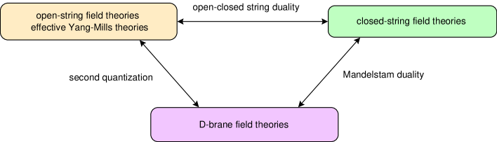
Fig. 2: A trinity of dualities: D-brane field theories point toward a third possible formulation of string theory treating D-branes as elementary excitations.

An expectation suggested here is that if we succeed in constructing an analog of the soliton operator for D particles in quantized closed string field theory, it would be described in the framework proposed in this paper. Recently, an attempt to construct a soliton operator for D-branes has been reported [18] within the framework of a special version (the so-called OSp-invariant string field theory) of closed string field theory. Unfortunately, however, it is difficult in the formulation of that work to see any signature of open-string degrees of freedom as collective coordinates of D-branes and the associated gauge structure. An appropriate understanding of this latter aspect in many-body D-brane systems should allow us to study the arrow on the right. An interesting problem is to determine what soliton operators look like in quantized closed string field theory of the type advocated in Ref. [4].

Conversely, we may attempt to derive closed string field theories starting from our D-particle field theory by developing a ‘bosonization’ technique for the D-brane fields. From this viewpoint, it would be interesting to investigate some suitable toy models as a warm-up exercise. Namely we may consider similar questions of a dual description for non-commutative solitons, where the classical solutions are known to exhibit a projector property, which is most probably related to the structure we have discussed, gives rise [14] to a Yang-Mills-like symmetry structure. In connection to this, it would also be interesting to study the BMN-type operators of the Yang-Mills theory of D-particles by using the present formalism. In our previous works, we have given some nontrivial predictions [19, 20] for the correlation functions of the BMN-type operators from supergravity via holography, which may be useful to determine the correspondence between our D-particle field theory and closed string field theories.

Finally, we touch on an interpretation of the peculiar base space of the present D-particle field theory. In terms of string theory, the infinite number of vector components $z^{i}_{n}$ and $\bar{z}^{i}_{n}$ correspond to the coordinates of a D-particle and infinite degrees of freedom representing possible open strings emanating from it. In this sense, the base-space coordinates describe certain fuzzy (permeable and osmotic) spatial domains. These open string degrees of freedom are latent in their nature, since they are activated only when acting on states, depending on the number of D-particles. This novel feature was taken into account by the projection conditions. In a broad sense, the D-particle field theory is somewhat reminiscent of the idea of ‘elementary domains’ [21] proposed by Yukawa in the late 1960s. Unlike the latter idea, where the non-locality is governed by the explicit form of extended domains, however, the non-locality in our theory caused by the open-string degrees of freedom is consistent with a more dynamical non-local structure of string theory as being characterized qualitatively by the space-time uncertainty relation [16]. This is responsible for the fact that D-particle Yang-Mills quantum mechanics encompasses general relativity, as we have demonstrated by deriving the 3-body gravitational force among D-particles in Ref. [22]. It would be very nice if we could see a more direct link to supergravity in our field-theory language.

Acknowledgements

A preliminary form of this paper was reported at the 21st Nishinomiya-Yukawa Memorial Symposium (YITP, Kyoto, November, 2006) and in the Komaba 2007 Workshop (Univ. of Tokyo, February, 2007). The author would like to thank the organizers and participants for their interest.

The present work is supported in part by Grants-in-Aid for Scientific Research [No. 13135205 (Priority Areas) and No. 16340067 (B)] from the Ministry of Education, Science and Culture of Japan, and also by the Japan-US Bilateral Joint Research Projects from JSPS.

References

-
[1]
M. Kaku and K. Kikkawa, Phys. Rev. D10 (1974)1110, 1823.
E. Cremmer and J. L. Gervais, Nucl. Phys. B90(1975)410. - [2] E. Witten, Nucl. Phys. B268(1986)157.
- [3] H. Hata, K. Itoh, T. Kugo, H. Kunitomo and K. Ogawa, Phys. Rev. D34 (1986)2360.
- [4] B. Zwiebach, Nucl. Phys. B390 (1993)33(hep-th/9206084).
- [5] For a recent important development, see M. Schnabl, Adv. Theor. Math. Phys. 10(2006)433 (hep-th/0511286) and references therein.
- [6] L. Rastelli, A. Sen and B. Zwiebach, Adv. Theor. Math. Phys. 5(2002)353 (hep-th/0012251).
-
[7]
S. R. Coleman, Phys. Rev. D11(1975)2088.
S. Mandelstam, Phys. Rev. D11(1975)3026. - [8] J. Schwinger, Phys. Rev. 128(1962)2425.
- [9] The first work on this system seems to be M. Claudson and M. Halpern, Nucl. Phys. B250(1985)689. It was then reinterpreted as a regularization of supermembrane in B. de Wit, J. Hoppe and H. Nicolai, Nucl. Phys. B305[FS23](1988)545. In the 1990s, the system was identified as a low-energy effective theory for D-particles in E. Witten, Nucl. Phys. B460(1996)335 .
- [10] T. Banks, W. Fschler, S. Shenker and L. Susskind, Phys. Rev. D55(1997)5112.
- [11] T. Yoneya, JHEP 12(2005)028 (hep-th/0510114).
- [12] A. Jevicki and B. Sakita, Nucl. Phys. B165(1980)511.
- [13] T. Yoneya, Nucl. Phys. B183 (1980)471.
- [14] See, e. g. J. A. Harvey, P. Kraus, F. Larsen and E. J. Martinec, JHEP 0007(2000)042 (hep-th/0005031) and references therein.
-
[15]
A. Jevicki and T. Yoneya, Nucl. Phys. B535(1998) 335 (
hep-th/9805069).
A. Jevicki, Y. Kazama and Y. Yoneya, Phys. Rev. D59(1999) 066001-1 (hep-th/9810146). - [16] T. Yoneya, Mod. Phys. Lett. A4(1989), 1587; Prog. Theor. Phys. 97(1989) 949 (hep-th/9703078). For an extensive review on this subject, see T. Yoneya, Prog. Theor. Phys. 103(2000) 1081 (hep-th/0004074).
- [17] See the second reference in [9].
- [18] Y. Baba, N. Ishibashi and K. Murakami, JHEP 0605(2006) 029(hep-th/0603152).
- [19] Y. Sekino and T. Yoneya, Nucl. Phys. B570(2000)174-206(hep-th/9907029).
- [20] M. Asano, Y. Sekino and T. Yoneya, Nucl. Phys. B678(2004) 197(hep-th/0308024).
- [21] Y. Katayama and H. Yukawa, Prog. Theor. Phys. Suppl. 41(1968)1.
- [22] Y. Okawa and T. Yoneya, Nucl. Phys. B535(1998) 335(hep-th/9805069); Nucl. Phys. B541(1999)163(hep-th/9808188 ).