Brownian Motion, “Diverse and Undulating”

Abstract

Truly man is a marvelously vain, diverse, and undulating object. It is hard to found any constant and uniform judgment on him. Michel de Montaigne, Les Essais, Book I, Chapter 1: “By diverse means we arrive at the same end”; in The Complete Essays of Montaigne, Donald M. Frame transl., Stanford University Press (1958).

Pour distinguer les choses les plus simples de celles qui sont compliquées et pour les chercher avec ordre, il faut, dans chaque série de choses où nous avons déduit directement quelques vérités d’autres vérités, voir quelle est la chose la plus simple, et comment toutes les autres en sont plus, ou moins, ou également éloignées. René Descartes, Règles pour la direction de l’esprit, Règle VI.

In order to distinguish what is most simple from what is complex, and to deal with things in an orderly way, what we must do, whenever we have a series in which we have directly deduced a number of truths one from another, is to observe which one is most simple, and how far all the others are removed from this-whether more, or less, or equally. René Descartes, Rules for the Direction of the Mind, Rule VI.

Car, supposons, par exemple que quelqu’un fasse quantité de points sur le papier à tout hasard, comme font ceux qui exercent l’art ridicule de la géomance. Je dis qu’il est possible de trouver une ligne géométrique dont la notion soit constante et uniforme suivant une certaine règle, en sorte que cette ligne passe par tous ces points, et dans le même ordre que la main les avaient marqués.

… Mais quand une règle est fort composée, ce qui luy est conforme, passe pour irrégulier.

G. W. Leibniz, Discours de métaphysique, H. Lestienne ed., Félix Alcan, Paris (1907).

Thus, let us assume, for example, that someone jots down a number of points at random on a piece of paper, as do those who practice the ridiculous art of geomancy. I maintain that it is possible to find a geometric line whose notion is constant and uniform, following a certain rule, such that this line passes through all the points in the same order in which the hand jotted them down.

… But, when the rule is extremely complex, what is in conformity with it passes for irregular.

G. W. Leibniz, Discourse on Metaphysics.

Mens agitat molem. Virgil, AEneid. lib. VI.

Un coup de dés jamais n’abolira le hasard. Stéphane Mallarmé, Cosmopolis, 1897.

A throw of the dice never will abolish chance.

L’antimodernisme, c’est la liberté des modernes. Antoine Compagnon, about his book “Les antimodernes : de Joseph de Maistre à Roland Barthes,” Bibliothèque des Idées, Gallimard, March 2005.

Antimodernism is the liberty of modern men.

Here we briefly describe the history of Brownian motion, as well as the contributions of Einstein, Sutherland, Smoluchowski, Bachelier, Perrin and Langevin to its theory. The always topical importance in physics of the theory of Brownian motion is illustrated by recent biophysical experiments, where it serves, for instance, for the measurement of the pulling force on a single DNA molecule.

In the second part, we stress the mathematical importance of the theory of Brownian motion, illustrated by two chosen examples. The by-now classic representation of the Newtonian potential by Brownian motion is explained in an elementary way. We conclude with the description of recent progress seen in the geometry of the planar Brownian curve. At its heart lie the concepts of conformal invariance and multifractality, associated with the potential theory of the Brownian curve itself.

Translation by Emily Parks and the author from the original French text

1 A brief history of Brownian motion

Several classic works give a historical view of Brownian motion. Amongst them, we cite those of Brush, Nelson, Nye, Pais, Stachel and Wax. We also cite a number of essays in mathematics, physics, especially those which have appeared very recently for the centenary of Einstein’s 1905 articles, and in biology.

1.1 Robert Brown

1.1.1 Brown’s observations and precursors

Robert Brown (1773-1858), of Scottish descent, was one of the greatest botanists of his time in Great Britain. He is renowned for his discovery of the nucleus of plant cells, for being the first to recognize the phenomenon of cytoplasmic streaming, and for the classification of several thousands dried plant specimens he brought back to England from a trip to Australia in 1801-1805.

In 1801 indeed, at the age of twenty-eight, he was chosen by Sir Joseph Banks as the botanist to accompany Matthew Flinders in the Investigator on the first circumnavigation of the Australian continent. The voyage was to extend over 5 years, and Brown used his time well, assembling substantial collections of plants, animals and minerals, and kept a diary.

Brown returned to England with his scientific reputation established. As said by Brown’s biographer, D. J. Mabberley, Brown’s Australian experiences and connections with the Continental schools of scientific thought moulded his research, with the result that he was recognized as one of the great European intellectuals of his day. Brown was called by Humboldt “Princeps Botanicorum.”

In a pamphlet, dated July 30th, 1828, first printed privately, then published in the Edinburgh New Philosophical Journal later that year, and republished several times elsewhere, entitled “A Brief Account of Microscopical Observations Made in the Months of June, July, and August, 1827, on the Particles Contained in the Pollen of Plants; and on the General Existence of Active Molecules in Organic and Inorganic Bodies,” Brown reported on the random movement of different particles that are small enough to be in suspension in water. It is an extremely erratic motion, apparently without end (see figure 1). A second article, dated July 28th, 1829, was published later and bears the brief title “Additional Remarks on Active Molecules.”

Brown used the wording active molecule in these titles in a sense different from its current one. It referred to earlier teaching of Georges-Louis Leclerc de Buffon (1707-1788) who introduced this word for the hypothetical ultimate constituents of the bodies of living beings. Only later with the acceptance and development of Dalton’s 1803 atomic theory the word molecule was going to take on its modern meaning.

The first plant Brown studied was Clarkia pulchella, whose pollen grains contain granules varying “from nearly $\frac{1}{4000}$ to about $\frac{1}{3000}$ of an inch in length, and of a figure between cylindrical and oblong, perhaps slightly flattened…” [from about six to eight microns]. It is these granules, not the whole pollen grains, upon which Brown made his observations. Concerning them, he wrote:

“While examining the form of these particles immersed in water, I observed many of them very evidently in motion; their motion consisting not only of a change of place in the fluid, manifested by alterations in their relative positions, but also not unfrequently of a change of form in the particle itself; a contraction or curvature taking place repeatedly about the middle of one side, accompanied by a correspondong swelling or convexity on the opposite side of the particle. In a few instances, the particle was seen to turn on its longer axis. These motions were such as to satisfy me, after frequently repeated observation, that they arose neither from currents in the fluid, nor from its gradual evaporation, but belonged to the particle itself.”

Figure 1: Brownian motion described by a pollen granule in suspension.

Brown made his observations just after the introduction of the first compound achromatic objectives for microscopes. Still, he used a simple microscope with a double convex lens, while he also possessed a pocket microscope with two lenses having a delicate adjustment:

“The observations, of which it is my intention to give a summary in the following pages, have all been made with a simple microscope, and indeed with one and the same lens, the focal length of which is about $\frac{1}{32}$nd of an inch.”

In fact, it is nowadays sufficient to look in a microscope to see small objects dancing.

Brown may have not been the first, however, to observe Brownian motion. In fact, he discussed in his second article (1829) previous observations by others which could have been interpreted as prior to his. The universal and irregular motion of small grains suspended in a fluid may have been observed soon after the discovery of the microscope.

The story begins with Anthony van Leeuwenhoek (1632-1723), a famous constructor of microscopes in Delft, who in 1676 was also designated executor of the estate of the no-less-famous painter Johannes Vermeer, who was apparently a personal friend. Leeuwenhoek built several hundred simple “microscopes,” with which he went as far as to observe living bacteria and discover the existence of spermatozoids.

In his second article, Brown then writes:

“I shall conclude these supplementary remarks to my former Observations, by noticing the degree in which I consider those observations to have been anticipated.

That molecular was sometimes confounded with animalcular motion by several of the earlier microscopical observers, appears extremely probable from various passages in the writings of Leeuwenhoek, as well as from a very interesting Paper by Stephen Gray, published in the 19th volume of the Philosophical Transactions.”

Next, one meets Needham, Buffon and Spallanzani, the 18th-century protagonists of the debate on spontaneous generation. Brown continues:

“Needham also, and Buffon, with whom the hypothesis of organic particles originated, seem to have not unfrequently fallen into the same mistake. And I am inclined to believe that Spallanzani, notwithstanding one of his statements respecting them, has under the head of Animalculetti d’ultimo ordine included the active Molecules as well as true Animalcules.”

Brown further cites Gleichen, “the discoverer of the motions of the Particles of the Pollen,” Wrisberg and Müller, who, having “adopted in part Buffon’s hypothesis, state the globules, of which they suppose all organic bodies formed, to be capable of motion;” and Müller, who “distinguishes these moving organic globules from real Animalcules, with which, he adds, they have been confounded by some very respectable observers.” Lastly, he cites a “very valuable Paper” published in 1814 by Dr. James Drummond, of Belfast, which “gives an account of the very remarkable motions of the spicula which form the silvery part of the choroid coat of the eyes of fishes,” and where “The appearances are minutely described, and very ingenious reasoning employed to show that, to account for the motions, the least improbable conjecture is to suppose the spicula animated.”

However, all these works had confined themselves to the examination of the particles of some organic bodies. Only Bywater, of Liverpool, is cited by Brown, in the same second article Additional Remarks on Active Molecules, for having stated in 1819 that “not only organic tissues, but also inorganic substances, consist of what he terms animated or irritable particles,” and therefore are subject to “Brownian motion.” However, Brown adds:

“I believe that in thus stating the manner in which Mr. Bywater’s experiments were conducted, I have enabled microscopical observers to judge of the extent and kind of optical illusion to which he was liable, and of which he does not seem to have been aware.”

As pointed out by R. M. Mazo, when citing the work by Van der Pas, there was, however, one predecessor that Brown overlooked. In July of 1784, Jan Ingen-Housz published a short article entitled Remarks on the use of the microscope, that contains the following lines:

“ … one must agree that, as long as the droplet lasts, the entire liquid and consequently everything which is contained in it, is kept in continuous motion by the evaporation, and that this motion can give the impression that some of the corpuscles are living, even if they have not the slightest life in them. To see clearly how one can deceive one’s mind on this point if one is not careful, one has only to place a drop of alcohol at the focal point of a microscope and introduce a little finely ground charcoal therein, and one will see these corpuscles in a confused continuous and violent motion as if they were animalcules which move violently around.”

However, although Ingen-Housz doubtless observed the motion, he ascribed it to evaporation and did not follow up his observation with any investigation of it.

Lastly, in 1827, one year before the publication by Brown, similar observations were also alluded to in France by the young Adolphe Brongniart (1801-1876), in a long Memoir for which he won a Prize in experimental physiology from the French Academy of Sciences. Brongniart’s findings about the motion of particles appear in a particular paragraph, followed by a note later annexed to his memoir. The note below reproduces the original passages.

It is interesting to notice that Brown actually discussed Brongniart’s work in detail in the last two pages of his famous 1828 article. There Brown first acknowledges that he was acquainted, before he engaged in his own inquiry in 1827, with the abstract of Brongniart’s work that was given to him by the author himself. He nevertheless stresses the lack in this work of observations of importance on the motion or form of the particles:

“Neither in the abstract referred to, nor in the body of the memoir which M. Brongniart has with great candour given in its original state, are there any observations, appearing of importance even to the author himself, on the motion or form of the particles […]”

But Brown adds about the note annexed by Brongniart in his article:

“Late in the autumn of 1827, however, M. Brongniart having at his command a microscope constructed by Amici, the celebrated professor of Modena, he was enabled to ascertain many important facts on both these points, the result of which he has given in the notes annexed to his memoir. On the general accuracy of his observations on the motions, form, and size of the granules, as he terms the particles, I place great reliance.”

This is followed by some criticism of more physiological relevance, to which Brongniart himself replied in a note added to the French translation of the same article by Brown in the Annales de Sciences Naturelles!

1.1.2 “Active Molecules” or Brownian motion?

Brown’s first publication on the erratic motion of the granules of pollen grains garnered much attention, but the use of the ambiguous terms “active molecules” by Brown brought him criticisms based on some misunderstanding. Indeed, under the influence of Buffon, the similar expression “organic molecules” represented hypothetical entities, elementary bricks all living beings would be made of. Such theories were still around at the beginning of the 19th century. In his famous first paper, Brown writes:

“ Reflecting on all the facts with which I had now become acquainted, I was disposed to believe that the minute spherical particles or Molecules of apparently uniform size, first seen in the advanced state of the pollen […] and lastly in bruised portions of other parts of the same plants, were in reality the supposed constituent or elementary Molecules of organic bodies, first so considered by Buffon and Needham, then by Wrisberg with greater precision, soon after and still more particularly by Müller, and, very recently, by Dr. Milne Edwards, who has revived the doctrine and supported it with much interesting detail.”

However, one of the substances he examined, silicified wood, once bruised still produced spherical particles, or molecules, in all respect like those mentioned before, and in such quantity, that, according to Brown,

“the whole substance of the petrifaction seemed to be formed of them. But hence I inferred that these molecules were not limited to organic bodies, not even to their products.

To establish the correctness of the inference, and to ascertain to what extent the molecules existed in mineral bodies, became the next body of inquiry. The first substance examined was a minute fragment of window-glass, from which, when merely bruised on the stage of the microscope, I readily and copiously obtained molecules agreeing in size, form, and motion with those which I had already seen. […]

Rocks of all ages, including those in which organic remains have never been found, yielded the molecules in abundance. Their existence was ascertained in each of the constituent minerals of granite, a fragment of the Sphinx being one of the specimens examined.”

In a word, in every mineral which I could reduce to a powder, sufficiently fine to be temporarily suspended in water, I found these molecules more or less copiously …”

His emphasis leads one to think that Brown’s opinion was that the observed particles themselves were animated. Faraday himself had to defend him during a Friday night lesson he gave at the Royal Society on February 21, 1829, about Brownian motion.

This led Brown in his Supplement Additional Remarks on Active Molecules to an apology:

“In the first place, I have to notice an erroneous assertion of more than one writer, namely, that I have stated the active Molecules to be animated. This mistake has probably arisen from my having communicated the facts in the same order in which they occurred, accompanied by the views which presented themselves in the different stages of the investigation; and in one case, from my having adopted the language, in referring to the opinion, of another inquirer into the first branch of the subject.

Although I endeavoured strictly to confine myself to the statement of the facts observed, yet in speaking of the active Molecules, I have not been able, in all cases, to avoid the introduction of hypothesis; for such is the supposition that the equally active particles of greater size, and frequently of very different form, are primary compounds of these Molecules, –a supposition which, though professedly conjectural, I regret having so much insisted on, especially as it may seem connected with the opinion of the absolute identity of the Molecules, from whatever source derived.”

Brown’s merit was in gradually emancipating himself from this misconception and in making a systematic study of the ubiquity of “active molecules,” hence of the movement named after him, with grains of pollen, dust and soot, pulverized rock, and even a fragment from the Great Sphinx! This served to eliminate the “vital force” hypothesis, where the movement was reserved to organic particles.

As for the nature of Brownian motion, even if Brown could not explain it, he eliminated easy explanations, like those linked to convection currents or to evaporation, by showing that the Brownian motion of a simple particle stayed “tireless” even in a isolated drop of water in oil! On the same occasion he eliminated as well the hypothesis of movements created by interactions between Brownian particles, a hypothesis that would nevertheless reappear later. He wrote in his Additional Remarks on Active Molecules:

“I have formerly stated my belief that these motions of the particles neither arose from currents in the fluid containing them, nor depended on that intestine motion which may be supposed to accompany its evaporation.

These causes of motion, however, either singly or combined with others, –as, the attractions and repulsions among the particles themselves, their unstable equilibrium in the fluid in which they are suspended, their hygrometrical or capillary action, and in some cases the disengagement of volatile matter, or of minute air bubbles,– have been considered by several writers as sufficiently accounting for the appearances. […] the insufficiency of the most important of those enumerated may, I think, be satisfactorily shown by means of a very simple experiment.

The experiment consists in reducing the drop of water containing the particles to microscopic minuteness, and prolonging its existence by immersing it in a transparent fluid of inferior specific gravity, with which it is not miscible, and in which evaporation is extremely slow. If to almond-oil, which is a fluid having these properties, a considerably smaller proportion of water, duly impregnated with particles, be added, and the two fluids shaken or triturated together, drops of water of various sizes […] will be immediately produced. Of these, the most minute necessarily contain but few particles, and some may be occasionally observed with one particle only. […] But in all the drops thus formed and protected, the motion of the particles takes place with undiminished activity, while the principal causes assigned for that motion, namely, evaporation, and their mutual attraction and repulsion, are either materially reduced or absolutely null.”

This ingenious experimental set-up gave him some hope of getting closer to the real cause of Brownian motion:

“By means of the contrivance now described for reducing the size and prolonging the existence of the drops containing the particles, which, simple as it is, did not till very lately occur to me, a greater command of the subject is obtained, sufficient perhaps to enable us to ascertain the real cause of the motions in question.”

Still, this real cause always eluded him. The theoretical picture formed perhaps by Brown, which however he always carefully avoided presenting as the conclusion of his studies, was that the particles of matter were animated into a rapid and irregular movement whose source was in the particles themselves and not in the surrounding fluid.

It is nevertheless fascinating to observe that in some instances he came close to the truth. One reads indeed in Microscopical Observations of Active Molecules the following striking remark:

“In Asclepiadeæ, strictly so called, the mass of pollen filling each cell of the anthera is in no stage separable into distinct grains; but within, its tesselated or cellular membrane is filled with spherical particles, commonly of two sizes. Both these kinds of particles when immersed in water are generally seen in vivid motion; but the apparent motions of the larger particle might in these cases perhaps be caused by the rapid oscillation of the more numerous molecules.”

This is precisely the correct explanation of the cause of the movement, if one mentally replaces the latter “numerous molecules,” i.e., the smaller granules as observed by Brown in this pollen, by the invisible numerous real molecules of the surrounding fluid!

In the same Princeps article, Brown also wondered whether the mobility of the particles existing in bodies was in any degree affected by the application of intense heat to the containing substance:

“… and in all these bodies so heated, quenched in water, and immediately submitted to examination, the molecules were found, and in as evident motion as those obtained from the same substances before burning.”

After heating of the substance, instead of a “quenching” of the latter in the fluid, had an “annealing” of the whole system been performed, which would have transferred heat to the surrounding fluid at equilibrium, an additional increase of Brownian activity with temperature would indeed have occurred!

The outstanding scientific stature of Brown brought him elogious comments. Before leaving Robert Brown, I cannot refrain from quoting first Mrs Charles Darwin, who said about a dinner party in 1839:

“Mr. Brown, whom Humboldt calls ‘the glory of Great Britain’ looks so shy, as if forced to shrink into himself, and disappear entirely.”

Finally, Charles Darwin gave, in his famous autobiographical notes written for his children, his own recollection from Brown in the late 1830’s:

“During this time [March 1837-January 1839] I saw also a good deal of Robert Brown; I used often to call and sit with him during his breakfast on Sunday mornings, and he poured forth a rich treasure of curious observations and acute remarks, but they almost always related to minute points, and he never with me discussed large or general questions in science. […]”

and

“I saw a good deal of Robert Brown, “facile Princeps Botanicorum,” as he was called by Humboldt. He seemed to me to be chiefly remarkable by the minuteness of his observations, and their perfect accuracy. His knowledge was extraordinarily great, and much died with him, owing to his excessive fear of ever making a mistake. He poured out his knowledge to me in the most unreserved manner, yet was strangely jealous on some points. I called on him two or three times before the voyage of the Beagle [1831-1836], and on one occasion he asked me to look through a microscope and describe what I saw. This I did, and believe now that it was the marvellous currents of protoplasm in some vegetable cell. I then asked him what I had seen; but he answered me, “That is my little secret.”

He was capable of the most generous actions. When old, much out of health, and quite unfit for any exertion, he daily visited (as Hooker told me) an old man-servant, who lived at a distance (and whom he supported), and read aloud to him. This is enough to make up for any degree of scientific penuriousness or jealousy.”

1.2 The period before Einstein

Between 1831 and 1857 it seems that one can no longer find references to Brown’s observations, but from the 1860’s forward his work began to draw large interest. It was noticed soon thereafter in literary circles, if we are to judge by a passage of “Middlemarch” published by George Eliot in 1872, where Rev. M. Farebrother offers to make an exchange to the surgeon Lydgate: “I have some sea-mice – fine specimens – in spirits. And I will throw in Robert Brown’s new thing – Microscopic Observations on the Pollen of Plants – if you don’t happen to have it already.”

Jean Perrin wrote in his famous 1909 memoir Brownian Motion and Molecular Reality:

“The singular phenomenon discovered by Brown did not attract much attention. It remained, moreover, for a long time ignored by the majority of physicists, and it may be supposed that those who had heard of it thought it analogous to the movement of the dust particles, which can be seen dancing in a ray of sunlight, under the influence of feeble currents of air which set up small differences of pressure or temperature. When we reflect that this apparent explanation was able to satisfy even thoughtful minds, we ought the more to admire the acuteness of those physicists, who have recognised in this, supposed insignificant, phenomenon a fundamental property of matter.”

1.2.1 Brownian motion and the kinetic theory of gases

It became clear from experiments made in various laboratories that Brownian motion increases when the size of the suspended particles decreases (one essentially ceases to observe it when the radius is above several microns), when the viscosity of the fluid decreases, or when the temperature increases. In the 1860’s, the idea emerged that the cause of the Brownian motion has to be found in the internal motion of the fluid, namely that the zigzag motion of suspended particles is due to collisions with the molecules of the fluid.

The first name worth citing in this regard is probably that of Christian Wiener, holder of the Chair of Descriptive Geometry at Karlsruhe, who in 1863 reaffirmed in the conclusions to his observations that the motion could be due neither to the interactions between particles, nor to differences in temperature, nor to evaporation or convection currents, but that the cause must be found in the liquid itself. That being so, his theory on atomic motion anticipated those of Clausius and Maxwell, implicating not only the motion of molecules but also the motion of “ether atoms”. The Brownian motion was thus bound to the vibrations of the ether, to the wavelength corresponding to that of red light and to the size of the smallest group of molecules moving together in the liquid. Such an explanation was criticized by R. Mead Bache, who showed that the motion was insensitive to the color of light, whether it was violet or red. Christian Wiener is nevertheless credited by some authors as the first to discover that molecular motion could explain the phenomenon.

At least three other people proposed the same idea: Giovanni Cantoni of Pavia, and two Belgian Jesuits, Joseph Delsaulx and Ignace Carbonelle. The Italian physicist attributed Brownian movement to thermal motions in the liquid:

“ In fact, I think that the dancing movement of the extremely minute solid particles in a liquid can be attributed to the different intrinsic velocities at a given temperature of both such solid particles and of the molecules of the liquid that hit them from every side.

I do not know whether others have already attempted this way of explaining Brownian motions…”

He concluded that :

“In this way Brownian motion, as described above, provides us with one of the most beautiful and direct experimental demonstrations of the fundamental principles of the mechanical theory of heat, making manifest the assiduous vibrational state that must exist both in liquids and solids even when one does not alter their temperature.”

The Belgian physicists published in the Royal Microscopical Society and in the Revue des Questions scientifiques, from 1877 to 1880, various Notes on the Thermodynamical Origin of the Brownian Movement. In a Note by Father Delsaulx, for example, one may read:

“The agitation of small corpuscles in suspension in liquids truly constitutes a general phenomenon,” that it is “henceforth natural to ascribe a phenomenon having this universality to some property of matter,” and that “in this train of ideas the internal movements of translation which constitute the calorific state of gases, vapours and liquids, can very well account for the facts established by experiment.”

Such a point of view, parallel to that of the kinetic theory of gases, faced strong opposition. One opponent, cytologist Karl von Nägeli of Switzerland, familiar with the kinetic theory of gases and the orders of magnitude involved, likewise the British chemist William Ramsey (the future Nobel laureate in Chemistry), commented that the particles in suspension have a mass several hundreds of millions of times larger than that of the molecules in the fluid. Each random collision with a molecule of the surrounding fluid produces therefore an effect far too small to displace the suspended particle. Nägeli wrote for example about a supposedly similar motion of micro-organisms in the air:

“The motion which a sun-mote, and on the whole any particle found in the air, can acquire by the collisions of an individual gas molecule or a multitude of such molecules is therefore so extraordinarily small, and the number of simultaneous collisions against the particle from all sides so extraordinarily large, that the particle behaves as if it were completely at rest.”

He believed instead that the cause of the motion was not the thermal molecular motion but some attractive or repulsive forces.

Nevertheless, the second part of his proposition about the frequency of such collisions held the principle of the solution. Because it is a collective statistical effect, as described in perspicacious manner by Father Carbonelle:

“In the case of a surface having a certain area, the molecular collisions of the liquid, which cause the pressure, would not produce any perturbation of the suspended particles, because these, as a whole, urge the particles equally in all directions. But if the surface is of area less than necessary to insure the compensation of irregularities, there is no longer any ground for considering the mean pressure; the inequal pressure, continually varying from place to place, must be recognised, as the law of large numbers no longer leads to uniformity; and the resultant will not now be zero but will change continually in intensity and direction. Further, the inequalities will become more and more apparent the smaller the body is supposed to be, and in consequence the oscillations will at the same time become more and more brisk…”

Perrin mentions these authors to conclude:

“These remarkable reflections unfortunately remained as little known as those of Wiener. Besides it does not appear that they were accompanied by an experimental trial sufficient to dispel the superficial explanation indicated a moment ago; in consequence, the proposed theory did not impress itself on those who had become acquainted with it.”

He continues:

“On the contrary, it was established by the work of M. Gouy (1888), not only that the hypothesis of molecular agitation gave an admissible explanation of the Brownian movement, but that no other cause of the movement could be imagined, which especially increased the significance of the hypothesis. This work immediately evoked a considerable response, and it is only from this time that the Brownian movement took a place among the important problems of general physics.”

Indeed in 1888 the French physicist Louis-Georges Gouy made the best observations on Brownian motion, from which he drew the following conclusions:

- The motion is extremely irregular, and the trajectory seems not to have a tangent.

- Two Brownian particles, even close, have independent motion from one another.

- The smaller the particles, the livelier their motion.

- The nature and the density of the particles have no influence.

- The motion is most active in less viscous liquids.

- The motion is most active at higher temperatures.

- The motion never stops.

Gouy seemed, however, to claim again that one cannot explain Brownian motion by disordered molecular motion, but only by the partially organized movements over the order of a micron within the liquid.

But somehow he became known as the “discoverer” of the cause of Brownian motion, as Jean Perrin wrote about his experimental conclusions:

“ Thus comes into evidence, in what is termed a fluid in equilibrium, a property eternal and profound. This equilibrium only exists as an average and for large masses; it is a statistical equilibrium. In reality the whole fluid is agitated indefinitely and spontaneously by motions the more violent and rapid the smaller the portion taken into account; the statical notion of equilibrium is completely illusory.”

1.2.2 Brownian motion and Carnot’s principle

Brownian agitation continues indefinitely. It does not contradict the principle of energy conservation, because any increase in the velocity of a grain, for instance, is accompanied by a local cooling of the surrounding fluid, and the thermal equilibrium is statistical.

Gouy was the first to note the apparent contradiction between Brownian motion and Carnot’s principle. The latter states that one cannot extract work from a simple source of heat. However, it really seems that some work is made, in a fluctuating manner, by the thermal motion of the molecules of the fluid. Gouy mentioned the theoretical possibility to extract work by a mechanism attached to a Brownian particle, and he concluded that Carnot’s principle perhaps was no longer valid for dimensions of the size of a micron, in that echoing Helmholtz’s reservations about the validity of such principle for living tissues.

These questions sparked the interest of Poincaré, who announced at the following lecture of the Congress of Arts and Sciences in St. Louis in 1904, about the “Present Crisis of Mathematical Physics”:

“But here the stage changes. Long ago the biologist, armed with his microscope, noticed in his specimens disorganized movements of small particles in suspension; that is the Brownian motion. He believed at first that it is a vital phenomenon, but soon he saw that inanimate bodies did not dance with less fervor than the others, so he handed it over to physicists. Unfortunately, physicists have been uninterested for a long while in this question; one concentrates light to enlighten the microscopic specimens, they thought; light does not go without heat, from which inhomogeneities of temperature, and then internal currents in the liquid that produce the motion we are speaking about..M. Gouy had the idea to look closer and he saw, or believed he saw that this explanation is unsustainable, that the motion becomes more lively the smaller the particles, but that they are not influenced by light. So, if the motion never stops, or more exactly is continually reborn without end, without an external source of energy, what are we to believe? We must not, without any doubt, renounce the conservation of energy because of this, but we see before our own eyes both motion transform into heat by friction, and inversely heat transform into motion; and all that while nothing is lost, as the motion lasts forever. This is the opposite of Carnot’s principle. If this is the case, to see the world develop in reverse, we no longer have need of the infinitely subtle eye of Maxwell’s demon, a microscope will suffice. The largest of bodies, those that have for example, a tenth of a millimeter, collide with atoms in motion from all sides, but they do not move at all as the shocks are so numerous that the law of chance says they compensate one another; however the smallest particles do not receive enough shocks for the compensation to be exact and they are unendingly tossed around. And voilà, one of our principles already in danger.”

It is rather subtle to prove that the Brownian phenomenon does not infringe on the impossibility of creating perpetual motion (called of the second kind), where work is extracted in a coherent manner by the observer (recalling Maxwell’s famous demon). One had to wait for Leo Szilard, who hinted in 1929 that, because of the amount of information required by such an attempt, the total produced entropy would compensate the apparent entropy reduction due to the coherent use of fluctuations. We shall briefly return to this question later, after having described Smoluchowski’s contributions.

1.2.3 The kinetic molecular “hypothesis”

Nowadays it seems evident to us that the world is made up of particles, of atoms and of molecules. However, it was not always the case, and the hypothesis of a continuous structure of matter was relentlessly defended until the end of the nineteenth century by famous names such as Duhem, Ostwald, and Mach.

The intuition or the idea that gases are composed of individual molecules was already present in the eighteenth century, and in 1738 David Bernoulli was probably the first to affirm that the pressure of a gas on its container is due to collisions of molecules with the walls. Avogadro made the radical affirmation in 1811 that equal volumes of two gases at the same pressure and same temperature contain the same number of molecules. When such conditions are of one atmosphere and of $25^{\rm o}$ Celsius, the number contained in a volume of 22.412 liters is noted as ${\mathcal{N}}$, and called Avogadro’s number.

To understand the stakes surrounding the determination of Avogadro’s number, one must recall that the constant $R$ in the perfect gas law has been experimentally accessible since the eighteenth century, thanks to the work of Boyle, Mariotte, Charles, and later Gay-Lussac. It is in fact associated to the number of moles, $N/{\mathcal{N}}$, which is an experimental macroscopic parameter, contrary to the total number of particles $N$, and Avogadro’s number ${\mathcal{N}}$, that are microscopic quantities.

The study of Brownian motion played an essential role in establishing the “molecular hypothesis” definitively. As Jean Perrin observed, the “hypothesis” that bodies, despite their homogeneous appearance, are made up of distinct molecules, in unending agitation which increases with temperature, is logically suggested by the phenomenon of Brownian motion alone, even before providing an explanation.

In fact, according to Perrin, what is really strange and new in Brownian motion, is, precisely, that it never stops, contrary to our every-day experience with friction phenomena. If, for example, we pour a bucket of water into a tub, the initial coherent motion possessed by the liquid mass disappears, de-coordinated by the multiple rebounds on the boundaries of the tub, until an apparent equilibrium settles within the fluid at rest. Does such a de-coordination of the motion of the particles proceed indefinitely, as it would in an ideal continuous medium? The answer by Perrin is exceptionally convincing:

“To have information on this point and to follow this de-coordination as far as possible after having ceased to observe it with the naked eye, a microscope will be of assistance, and microscopic powders will be taken as indicators of the movement. Now these are precisely the conditions under which the Brownian motion is perceived: we are therefore assured that the de-coordination of motion, so evident on the ordinary scale of our observations, does not proceed indefinitely, and on the scale of microscopic observation, we establish an equilibrium between coordination and de-coordination. If, that is to say, at each instant, certain of the indicating granules stop, there are some in other regions at the same instant, the movement of which is re-coordinated automatically by their being given the speed of granules which have come to rest. So that it does not seem possible to escape the following conclusion:

Since the distribution of motion in a fluid does not progress indefinitely, and is limited by a spontaneous re-coordination, it follows that the fluids are themselves composed of granules or molecules, which can assume all possible motions relative to one another, but in the interior of which dissemination of motion is impossible. If such molecules had no existence it is not apparent how there would be any limit to the de-coordination of motion […] In brief, the examination of Brownian movement alone suffices to suggest that every fluid is formed of elastic molecules, animated by perpetual motion.”

In 1905 Albert Einstein was the first, actually along with (but independently from) William Sutherland from Melbourne, to propose a quantitative theory of Brownian motion. This theory will allow Perrin to determine the precise value of Avogadro’s number ${\mathcal{N}}$, in his famous experiments of 1908-1909. Sutherland and Einstein succeeded where many others failed, because they used an ingenious and global reasoning of statistical mechanics, that we will explain here. Marian von Smoluchowski made at the same time an analysis according to a different “Gedankenweg,” more probabilistic, which led him to similar conclusions. We will came back to this point later in the paper.

1.3 William Sutherland, 1904-05

In his famous biography of Einstein, Subtle is the Lord… (1982), Abraham Pais noted, while describing Einstein’s route to his well-known diffusion relation, that the same relation had been discovered “at practically the same time” by the Melbourne theoretical physicist William Sutherland, following similar reasoning to Einstein’s, and had been submitted for publication to the Philosophical Magazine in March 1905, shortly before Einstein completed the doctoral thesis in which he first announced the relation. Pais, therefore, proposed that the relation be called the “Sutherland-Einstein relation”.

We follow here the introduction of the essay, Speculating about Atoms in Early 20th-century Melbourne: William Sutherland and the ‘Sutherland-Einstein’ Diffusion Relation, written recently by the Australian historian of science Rod W. Home. In this section we shall briefly discuss Sutherland’s work, and the factors that may have led to his work having been over-shadowed by Einstein’s, and soon forgotten. When the Einstein International Year of Physics commemorates the hundredth anniversary of the Annus Mirabilis papers’ release, focusing also on W. Sutherland’s achievements seems to be just fair!

1.3.1 Sutherland’s papers

Sutherland’s paper to which Pais refers was actually published in June 1905, after Einstein completed his thesis, but shortly before he submitted it for examination. We seem to be looking here at a perfect example of effectively simultaneous discovery. However, as Rod Home notes, the story is still a little more complicated, for Sutherland had already reported his derivation over a year earlier, at the congress of the Australasian Association for the Advancement of Science held in Dunedin, New Zealand, in January 1904, and his paper had been published in the congress proceedings in early 1905! Unfortunately, there was a misprint in the crucial equation giving the diffusion coefficient of a large molecular mass in terms of physical parameters: Avogadro’s constant was missing!

The correct and extended equation, finally published in the Philosophical Magazine, is

$$D=\frac{RT}{\mathcal{N}}\frac{1}{6\pi\eta\,a}\frac{1+3\eta/\beta a}{1+2\eta/\beta a},$$ (1)

where $R$ is the perfect gas constant, $T$ the absolute temperature, $\mathcal{N}$ Avogadro’s number, $\eta$ the fluid viscosity, $a$ the radius of the (spherical) diffusing molecule, and $\beta$ the coefficient of sliding friction if there is slip between the diffusing molecule and the solution. To deal with the available empirical data, Sutherland had indeed to allow for a varying coefficient of sliding friction between the diffusing molecule and the solution. By taking $\beta$ to infinity, so there is no slip at the boundary, one recovers the usual form of the equation:

$$D=\frac{RT}{\mathcal{N}}\frac{1}{6\pi\eta\,a}.$$ (2)

Since in a fluid the molecules are close packed the molecular radius $a$ should be proportional to the cube root of the molar volume ${\mathcal{B}}$, the volume occupied by Avogadro’s number of particles. Hence, from the constancy of the product $aD$ in relation (2), should follow that of ${\mathcal{B}}^{1/3}D$. After having estimated this constant from experimental data on the diffusion of various dissolved substances, Sutherland could obtain the molar volume of albumin, and got an estimate of its atomic mass as 32814 Da.

1.3.2 Sutherland, Einstein and Besso

In 1903, Einstein and his friend Michele Besso discussed a theory of dissociation that required the assumption of molecular aggregates in combination with water, the “hypothesis of ionic aggregates,” as Besso called it. This assumption opens the way to a simple calculation of the sizes of ions in solution, based on hydrodynamical considerations. In 1902, Sutherland had considered in Ionization, Ionic Velocities, and Atomic Sizes a calculation of the sizes of ions on the basis of Stokes’ law, but criticized it as in disagreement with experimental data. The very same idea of determining sizes of ions by means of classical hydrodynamics occurred to Einstein in his letter of 17 March 1903 to Besso, where he proposed what appears to be just the calculation that Sutherland had performed:

“Have you already calculated the absolute magnitude of ions on the assumption that they are spheres and so large that the hydrodynamical equations for viscous fluids are applicable? With our knowledge of the absolute magnitude of the electron [charge] this would be a simple matter indeed. I would have done it myself but lack the reference material and time; you could also bring in diffusion in order to obtain information about neutral salt molecules in solution.”

As the editors of Einstein’s Collected Papers remark, “This passage is remarkable, because both key elements of Einstein’s method for the determination of molecular dimensions, the theories of hydrodynamics and diffusion, are already mentioned, although the reference to hydrodynamics probably covers only Stokes’ law”.

It is also striking that an earlier letter of 11-17 February 1903, this time from Besso to Einstein, clearly indicates that they had been discussing Sutherland’s work together. This letter contains two parts. The first deals with experimental data in connection to the dissociation of bi-ionic molecules. The second discusses what Besso calls “Sutherland’s hypothesis,” in connection to dissociation or dissolution. He states that the theory of “ionic hydrates,” as he calls it, rescues temporarily this hypothesis with regard to Ostwald’s dilution law. Since Besso also discusses the role of imperfect semi-permeable membranes as a possible experimental test of Sutherland’s hypothesis, P. Speziali, in the French edition of the Einstein-Besso correspondence, has indicated that Besso would have been discussing in this letter another of Sutherland’s papers, entitled “Causes of osmotic pressure and of the simplicity of the laws of dilute solutions.”

However, upon reading these letters of 1903, one cannot refrain from wondering whether Besso and Einstein were not also acquainted with and discussing Sutherland’s 1902 paper on ionic sizes. In that case, Sutherland suggestion to use hydrodynamic Stokes’ law to determine the size of molecules would have been a direct inspiration to Einstein’s dissertation and subsequent work on Brownian motion!

1.3.3 Sutherland’s legacy

That Sutherland, in spite of his isolation in Melbourne, was well-known in physics circles is also evidenced by the fact that he was invited to contribute to the Boltzmann Festschrift in 1904 –the only other non-European contributor being J. Willard Gibbs!– If so, why did Einstein and not Sutherland become famous?

Sutherland had assumed the existence of atoms, and attacked a practical question, the measurement of large molecular masses. He was interested in these masses because of their role in the chemical analysis of organic substances. While that is what everyone now uses the Sutherland-Einstein equation for, it was perhaps not of so widespread interest at the time. However, we have just seen from the Einstein-Besso correspondence how extremely important Sutherland’s idea was of determining the sizes of ions or molecules by means of classical hydrodynamics.

On the other hand, as stressed by the editors of The Collected Papers:

“In developing in his dissertation a new method for the determination of molecular dimensions, Einstein was concerned with several problems on different levels of generality. An outstanding current problem of the theory of solutions was whether molecules of the solvent are attached to the molecules or ions of the solute. Einstein’s dissertation contributed to the solution of this problem. He recalled in 1909:

“At the time I used the viscosity of the solution to determine the volume of sugar dissolved in water because in this way I hoped to take into account the volume of any attached water molecule.”

The results obtained in his dissertation indicate that such an attachment does occur. Einstein’s concerns extended beyond this particular question to more general problems of the foundations of the theory of radiation and the existence of atoms. He later emphasized:

“A precise determination of the size of the molecules seems to me of the highest importance because Planck’s radiation formula can be tested more precisely through such a determination than through measurements on radiation.”

The dissertation also marked the first major success in Einstein’s effort to find further evidence for the atomic hypothesis, an effort that culminated in his explanation of Brownian motion.”

To conclude, it is probably most appropriate to cite R. W. Home:

“Of course, the diffusion-viscosity relation is generally known as the Einstein relation, not the Sutherland-Einstein relation. Why? In part, I think, this happened because in the early 20th century, theoretical physics was a largely German affair. In so far as the relation was taken up, and initially it was not taken up much at all, it was taken up by Continental researchers who had read Einstein’s work but failed to notice that the relation was also buried in a paper in the Philosophical Magazine entitled “A dynamical theory for non-electrolytes and the molecular mass of albumin.” In the English-speaking world, where the Philosophical Magazine was one of the leading journals in the field, there were very few people pursuing theoretical physics in the German style. There is plenty of testimony that experimentally orientated British physicists were at something of a loss as how to assess Sutherland’s work. His obituary in Nature makes the point very clearly:

“His papers are well known to the scientific world. They are distinguished by great width of reading in the latest phases of the subjects he treated, combined with very bold speculation always brought into ample comparison with experimental knowledge. His generalisations were, indeed, so numerous that it was often a difficult task to try to estimate their value.”

So in Britain, Surtherland didn’t have a readership likely to be alert to the significance of his announcement of a relationship between diffusion and viscosity, in the way some Continental readers of Einstein’s work were. And, finally, Sutherland’s own presentation surely would not have helped, with the relation itself being almost submerged by his lengthy computations relating to the molecular mass of albumin. He would have done much better to highlight the relation, alone, in a paper to itself. But that was not his style! His mind was firmly fixed on the problem of determining molecular masses of large molecules, and he clearly saw the diffusion-viscosity relation as an incidental result arrived at on the way to achieving that larger goal, not as something of particular value in its own right.”

In this year 2005, it is definitely time, I think, for the physics community to finally recognize Sutherland’s achievements, and following Pais’ suggestion, to re-baptize the famous relation (2) with a double name!

1.4 Albert Einstein, 1905

Mens agitat molem

1.4.1 Einstein’s Dissertation

One finds nowadays in the literature excellent descriptions of Einstein’s dissertation. An outstanding presentation is given in the Editorial Notes of the Collected Papers of Albert Einstein. Their presentation is closely followed in this section, which incorporates some material of the editorial notes of the chapter entitled “Einstein’s dissertation on the determination of molecular dimensions.” The interested reader can also find a detailed scientific study of Einstein’s doctoral thesis in a recent article by Norbert Straumann.

Einstein completed his dissertation on “A New Determination of Molecular Dimensions” on 30 April 1905, and submitted it to the University of Zürich on 20 July. Shortly after being accepted there, the manuscript was sent for publication to the Annalen der Physik, where it would be published in 1906. On 11 May 1905, eleven days after finishing his thesis, Einstein had also sent the manuscript of his first paper on Brownian motion to the Annalen, which would publish it on 18 July 1905.

Einstein’s central assumption is the validity of using classical hydrodynamics to calculate the effect of solute molecules, treated as rigid spheres, on the viscosity of the solvent in a dilute solution. His method is well suited to determine the size of solute molecules that are large compared to those of the solvent, and he applied it to solute sugar molecules. As we have seen above, Sutherland published in 1905 a method for determining the masses of large molecules, with which Einstein’s method shares many important elements. Both methods make use of the molecular theory of diffusion that Nernst developed on the basis of van ’t Hoff’s analogy between solutions and gases, and of Stokes’ law of hydrodynamic friction.

The first of the results in the dissertation is a relation between the coefficients of viscosity of a liquid with and without suspended molecules ($\eta^{*}$ and $\eta$, respectively),

$$\eta^{*}=\eta\left(1+{{\left[{5}/{2}\right]}}\,\varphi\right),$$ (3)

where $\varphi$ is the fraction of the volume occupied by the solute molecules. [The correct coefficient $[\frac{5}{2}]$ appeared later (see below).]

The second result is the famous expression (2) for the coefficient of diffusion $D$ of the solute molecules. Like Loschmidt’s method based on the kinetic theory of gases, the expressions obtained by Einstein give two equations for two unknowns, Avogadro’s number $\mathcal{N}$, and the molecular radius $a$ of the suspended particles, hence providing a possible determination of molecular dimensions!

The derivation of eq. (3) represents the technically difficult part of Einstein’s dissertation. It rests on the assumption that the motion of the fluid can be described by the hydrodynamical equations for stationary flow of an incompressible homogeneous fluid, even in the presence of solute molecules; that the inertia of these molecules can be neglected; that they do not interact; and that they can be treated as rigid spheres moving in the liquid without slipping, under the sole influence of hydrodynamical stress.

Eq. (2) follows from the conditions of dynamical and thermodynamical equilibrium in the fluid. Its derivation, as does Sutherland’s, requires the identification of the force on a single large molecule, which appears in Stokes’ law, with the apparent force due to the osmotic pressure. We shall return to this derivation in detail in the next section, when describing the content of Einstein’s first paper on Brownian motion. In the dissertation, Einstein’s derivation of eq. (2) does not involve yet the theoretical tools he developed in his work on the statistical foundations of thermodynamics in the preceding years. Here he simply states the osmotic pressure law, while in his first paper on Brownian motion, he will instead derive from first principles the validity of van ’t Hoff’s law for large suspended particles.

In 1909, Einstein drew Perrin’s attention to his method for determining the size of solute molecules, which allows one to take into account the volume of any water molecule attached to the latter, and he suggested its application to the suspensions studied by Perrin in relation to Brownian motion. In the following year, an experimental study of formula (3) for the viscosity coefficient was performed by a pupil of Perrin, Jacques Bancelin. Using the same aqueous emulsions of gum-resin (“gamboge”), he confirmed that the increase in viscosity does not depend on the size of the solute molecules, but only on their volume fraction. However, the coefficient of $\varphi$ in eq. (3) was found to be close to 3.9, instead of the predicted value 1. That prompted Einstein, after an unsuccessful attempt to find an error, to ask his student and collaborator Ludwig Hopf to check his calculations and arguments:

“I have checked my previous calculations and arguments and found no error in them. You would be doing a great service in this matter if you would carefully recheck my investigation. Either there is an error in the work, or the volume of Perrin’s substance in the suspended state is greater than Perrin believes.”

Hopf did find an error in the dissertation, namely in the derivatives of some velocity components, and obtained for $\varphi$ a corrected coefficient 2.5. The remaining discrepancy between this corrected theoretical factor and the experimental one led Einstein to suspect that there might be also an experimental error.

In early 1911 Einstein submitted his correction for publication, and recalculated Avogadro’s number. He obtained a value of $6.56\times 10^{23}$ per mole, a value that is close to those derived from kinetic theory and Planck’s black-body radiation theory.

The paper published in 1911 by Bancelin in the Comptes rendus de l’Académie des Sciences gave an experimental value of 2.9 as the coefficient of $\varphi$ in eq. (3). Extrapolating his results to sugar solutions, Bancelin recalculated Avogadro’s number, and found a value of $7.0\times 10^{23}$ per mole.

Einstein’s dissertation was at first overshadowed by his more spectacular work on Brownian motion, and it required an initiative by Einstein to bring it to the attention of the scientists of his time. The paper on Brownian motion, the first of several on this subject that Einstein published over the course of the next couple of years, actually included his first published statement of the famous relationship linking diffusion with viscosity, that he had derived in his thesis.

As Abraham Pais points out in Subtle is the Lord…, this equation has found widespread applications, as a result of which Einstein’s January 1906 paper in the Annalen der Physik, the published version of his dissertation, later became his most frequently cited paper! As stressed by R. H. Home in his essay on Sutherland, Pais also goes on to argue that the thesis was also one of Einstein’s “most fundamental papers”, of comparable intrinsic significance to the other papers Einstein wrote in that year of 1905. “In my opinion,” Pais writes, “the thesis is on a par with [Einstein’s] Brownian motion article”: indeed, “in some if not all respects, his results are by-products of his thesis work.”

It is now time to turn to this famous 1905 Brownian motion article.

1.4.2 The 1905 article on Brownian motion

The 1905 article is entitled: “On the Motion of Small Particles Suspended in Liquids at Rest, Required by the Molecular-Kinetic Theory of Heat.” There, Einstein tried to establish the existence and the size of molecules, and to determine a theoretical method for computing Avogadro’s number precisely, by using the molecular kinetic theory of heat. In fact, he concluded:

“Möge es bald einem Forscher gelingen, die hier aufgeworfene, für die Theorie der Wärme wichtige Frage zu entscheiden !”

Astonishingly enough, he was not yet certain that one could apply it to Brownian motion. In fact, his introduction opens with: “In this paper it will be shown that, according to the molecular-kinetic theory of heat, bodies of a microscopically visible size suspended in liquids must, as a result of thermal molecular motions, perform motions of such magnitude that they can be easily observed with a microscope. It is possible that the motions to be discussed here are identical with so-called Brownian molecular motion; however the data available to me on the latter are so imprecise that I could not form a judgement on the question.”

Einstein relied on the results of his thesis, that he completed eleven days before submitting his famous article on the suspensions of particles. Only later would his predictions be progressively confirmed by refined experimental data on Brownian motion.

1.4.3 The Einstein-Sutherland derivation

The demonstration is based on two distinct elements from apparently contradicting domains.

It seemed initially natural to use a hydrodynamic representation for particles in suspensions with size much greater than that of the liquid’s molecules. A substantial amount of knowledge on the subject was available, in particular the famous “Stokes’ formula,” which gives the force of friction opposing to a sphere moving in the liquid.

But at the same time it was necessary for Einstein to exploit the kinetic theory of heat, pulling it away from the original context of the theory of gases and bringing it closer to the context of liquids, where the state of the theory was much less advanced. It was the crucial notion of osmotic pressure, developed by van ’t Hoff, that made the passage possible. It is based on the concept of kinetic molecular disorder, where solute molecules, with a size comparable to that of the liquid’s molecules, participate to the general motion like in a dilute gas.

Einstein was in possession of two theories about particles in a fluid. The first: Stokes’ hydrodynamic theory, based on the hypothesis that a liquid is a continuous medium which adheres to a large solid surface moving through it, without any turbulence, and where the molecular agitation does not seem to play any role. The other: van ’t Hoff’s osmotic theory, based on the hypothesis that a particle in solution is similar to any other fluid molecule, and therefore is subjected to the same laws of molecular agitation.

One needed Einstein’s perspicacity and his profound knowledge of statistical mechanics to understand and to prove that the two points of view were simultaneously valid for particles as big as Brownian particles.

Einstein first studied the osmotic pressure created in the solution by solute molecules. This notion was developed by J. H. van ’t Hoff who, for dilute solutions, showed the identity between the pressure exerted on semi-permeable walls by molecules in solution and the partial pressure exerted by a gas. For sufficiently dilute solutions, this additional pressure $p$ due to the molecules in solution satisfies the law of perfect gases

$$p=\frac{n}{\mathcal{N}}R\,T,$$ (4)

where $R$ is the ideal gas constant, $T$ is the absolute temperature, and $n$ is the number of solute particles per unit volume, or particle density.

In his thesis, Einstein considered the effect of the density of such molecules on the viscosity, such as in the case of sugar in water. This time the particles in suspension are much larger so as to be observable under a microscope. Einstein right away affirms that the difference between solute molecules and particles in suspension is only a matter of size, and that van ’t Hoff’s law must be applied as well to particles in suspension. Next, he proves this fact and formula (4), by determining the free energy of an ensemble of such particles in suspension. In fact, he calculates the associated partition function by the phase space method.

Einstein then imagines that the numerous particles of the suspension are subjected to an external force $F$, which may depend on their positions but not on time. This force, acting along the $x$ axis for instance, moves each particle of the solute, and generates a gradient of concentration. Let $n(x,y,z;t)$ be the number of particles in suspension per unit volume around the point $x,y,z$ at the instant $t$. From (4), a non-uniform osmotic pressure corresponds to a gradient of concentration of particles in suspension. By considering the resultant of all pressure forces on an elementary interval ${\rm d}x$, one also obtains the force of the osmotic pressure per unit volume:

$$\Pi=-\frac{\partial p}{\partial x}=-{\rm grad}\,p=-\frac{R}{\mathcal{N}}\,T{\rm grad}\,n(x,y,z;t),$$ (5)

where here the gradient is the spatial derivative in the direction $x$ of the force.

In addition, the quantity $\Pi_{F}=n\,F$ represents the total external force per unit volume acting on the Brownian particles in suspension. From both a hydrostatic and thermodynamic point of view, one imagines a priori that the equilibrium of a unit of volume of the suspension is established when the force $\Pi_{F}$ is balanced by the osmotic pressure force $\Pi$. In fact, by using arguments of equilibrium invariance of the free energy with respect to virtual displacements, Einstein demonstrates that actually the sum of the external and osmotic forces per unit volume cancels:

$$\Pi_{F}+\Pi = 0,$$ (6)

$$n\,F = \frac{R}{\mathcal{N}}\,T{\rm grad}\,n.$$ (7)

One notices that he directly obtained the explicit formula (7) from the free energy of the particles in suspension, without relying on the result (4), which shows the two results come from the same approach.

The second part of this argument focuses on the dynamics of the flux equilibrium. Equilibrium in the fluid is actually just an apparent effect: while the force $F$ moves the particles in suspension, these are also subjected to Brownian motion which reflects the kinetic nature of heat.

By moving in the liquid under the force $F$, each particle in suspension experiences an opposing force of viscous friction. This brings the particle to a limit velocity $V=~{}F/\mu$, where $\mu$ is the coefficient of viscous friction for each particle in suspension. The result is a flux of particles

$$\Phi_{F}=n\,V=n\,F/\mu,$$ (8)

that is the number of particles crossing a unit surface perpendicular to the direction $x$ of the force.

The particle density $n(x,y,z;t)$ satisfies the local diffusion equation

$$\frac{\partial n}{\partial t}=D\Delta n,$$ (9)

where $\Delta$ is the Laplacian $\Delta=\frac{\partial^{2}}{\partial x^{2}}+\frac{\partial^{2}}{\partial y^{2}}+\frac{\partial^{2}}{\partial z^{2}},$ and where $D$ is a coefficient, called the coefficient of diffusion, measured in square meters per second units. To this equation is naturally associated a diffusion flux $\Phi_{D}$, which is the number of particles diffusing across a unit surface per unit of time. This flux is directly connected to the concentration gradient by

$$\Phi_{D}=-D\,{\rm grad}\,n.$$ (10)

At equilibrium, here both local and dynamic, the force-driven flux $\Phi_{F}$ (8) and the flux of diffusion $\Phi_{D}$ (10), cancel:

$$\Phi_{F}+\Phi_{D} = 0,$$ (11)

$$n\,F/\mu = D\,{\rm grad}\,n.$$ (12)

By comparing the static equation (7) and the dynamic equation (12), one sees that they have identical structures for the dependence on $n$ and its gradient, from which we obtain the required identity between the coefficients:

$$D=\frac{1}{\mu}\frac{RT}{\mathcal{N}}.$$ (13)

By supposing that the particles in suspension are all spheres of radius $a$, Einstein uses at last Stokes’ relation which gives the coefficient of friction $\mu$ of a sphere immersed in a (continuous) fluid with viscosity $\eta$:

$${\mu}=6\pi\eta\,a,$$ (14)

from which he finally deduced:

$$D=\frac{RT}{\mathcal{N}}\frac{1}{6\pi\eta\,a}.$$ (15)

This is Einstein’s famous relation, which is already in his thesis. In fact, as mentioned above, the same relation was discovered earlier in Australia and, by a remarkable coincidence, published at practically the same moment as Einstein was working on his thesis. William Sutherland published his Philosphical Magazine article in March of 1905. One should therefore definitely call this relation the Sutherland-Einstein relation.

In the 1905 article, Einstein completes these results by means of mathematical and probabilistic considerations. Let $P(x,y,z;t)$ be the probability density of finding a Brownian particle at a point $x,y,z$ at the time $t$. This density satisfies the diffusion equation:

$$\frac{\partial P}{\partial t}=D\,\Delta P.$$ (16)

Let us follow Einstein in his demonstration.

He starts by introducing a time interval $\tau$, small compared to the duration of the observation, but large enough for the motions made by a particle during two consecutive intervals of time $\tau$ to be considered as independent events. Let us suppose then that in a liquid suspension there is a total number of particles $N$. During the time interval $\tau$, the coordinates of each particle along the $x$ axis will change by an amount $\Delta$, where $\Delta$ takes a different value (positive or negative) for each particle. A probability distribution governs $\Delta$: the number ${\rm d}N$ of particles with a displacement between $\Delta$ and $\Delta+{\rm d}\Delta$ is:

$${\rm d}N=N\varphi_{\tau}(\Delta){\rm d}\Delta,$$

where

$$\int_{-\infty}^{+\infty}\varphi_{\tau}(\Delta){\rm d}\Delta=1,$$ (17)

and where, for small $\tau$, $\varphi_{\tau}(\Delta)$ differs from zero only for very small values of $\Delta$. This function also satisfies the symmetry condition

$$\varphi_{\tau}(\Delta)=\varphi_{\tau}(-\Delta).$$ (18)

Einstein tries then to determine how the coefficient of diffusion depends on $\varphi$, once again by considering only the unidimensional case where the particle density $n$ depends only on $x$ and $t$. We can thus write $n=f(x,t)$ (the number of particles per unit volume) and we calculate the particle distribution at the time $t+\tau$ given the distribution at the time $t$. From the definition of the function $\varphi_{\tau}(\Delta)$, we obtain the number of particles between two planes in $x$ and $x+{\rm d}x$ at the time $t+\tau$:

$$f(x,t+\tau){\rm d}x={\rm d}x\int_{-\infty}^{+\infty}f(x+\Delta,t)\varphi_{\tau}(\Delta){\rm d}\Delta.$$ (19)

Since $\tau$ is very small, we can assume that

$$f(x,t+\tau)=f(x,t)+\tau\frac{\partial f}{\partial t}.$$ (20)

Moreover, expand $f(x+\Delta,t)$ in powers of $\Delta$:

$$f(x+\Delta,t)=f(x,t)+\Delta\frac{\partial f(x,t)}{\partial x}+\frac{\Delta^{2}}{2}\frac{\partial^{2}f(x,t)}{\partial x^{2}}+\cdots$$

We can then substitute such an expansion inside the integral in (19) as only very small values of $\Delta$ contribute to the latter. We obtain:

$$f+\tau\frac{\partial f}{\partial t}=f\times\int_{-\infty}^{+\infty}\varphi_{\tau}(\Delta){\rm d}\Delta+\frac{\partial f}{\partial x}\times\int_{-\infty}^{+\infty}\Delta\varphi_{\tau}(\Delta){\rm d}\Delta+\frac{\partial^{2}f}{\partial x^{2}}\times\int_{-\infty}^{+\infty}\frac{\Delta^{2}}{2}\varphi_{\tau}(\Delta){\rm d}\Delta+\cdots$$

On the right side, the second term, fourth term, etc., cancel out because of the parity property (18), while each of the other terms is very small in relation to the preceding one. From this equation, taking into account the conservation property (17), defining

$$\frac{1}{\tau}\int_{-\infty}^{+\infty}\frac{\Delta^{2}}{2}\varphi_{\tau}(\Delta){\rm d}\Delta=D$$ (21)

and keeping only the first and the third terms on the right hand side, we obtain

$$\frac{\partial f}{\partial t}=D\frac{\partial^{2}f}{\partial x^{2}}.$$ (22)

This is the famous diffusion equation, where the diffusion coefficient $D$ is given by (21).

We comment now on the method of Einstein. The definition (21) of the diffusion coefficient $D$ can be rewritten as

$$\langle\Delta^{2}\rangle_{\tau}\equiv\int_{-\infty}^{+\infty}\Delta^{2}\varphi_{\tau}(\Delta){\rm d}\Delta=2D\tau,$$ (23)

which is the average quadratic variation produced by the thermal agitation during the time $\tau$. Formally identical to formula (28) (see below), which gives the law of the average quadratic displacement as a function of time, it somehow contains the latter tautologically. Moreover, as $\tau$ is assumed to be small, this definition implies the existence of the limit (21) for $\tau\to 0$, if one requires $D$ to be independent of $\tau$.

Einstein continues by noting that until then all particles have been considered with respect to a common origin on the $x$ axis, but that their independence also allows us to consider each particle with respect to the position it occupied at the time $t=0$. Therefore $f(x,t)\,{\rm d}x$ is also the number of particles (per unit area) whose abscissa $x$ has changed by an amount comprised between $x$ and $x+{\rm d}x$, over the time interval from $0$ to $t$. The function $f$ then obeys the diffusion equation (22). Einstein also says that evidently one must have, for $t=0$,

$$f(x,t=0)=0,\forall x\neq 0\,;\,\,\,\,{\rm and}\int_{-\infty}^{+\infty}f(x,t){\rm d}x=N.$$

The problem thus coincides with that of diffusion from a given point (neglecting the interactions between diffusing particles), and is now entirely determined mathematically; its solution is:

$$f(x;t)=\frac{N}{(4\pi Dt)^{1/2}}\exp{\left(-\frac{x^{2}}{4Dt}\right)}.$$ (24)

The probability density $P(x,t)=f(x,t)/N$ for a Brownian particle to be within ${\rm d}x$ of $x$, assuming it was at $x=0$ at the instant $t=0$, is thus the normalized Gaussian distribution

$$P(x;t)=\frac{1}{(4\pi Dt)^{1/2}}\exp{\left(-\frac{x^{2}}{4Dt}\right)}.$$ (25)

In three dimensions, if the Brownian particle is at $\vec{0}$ at the instant $t=0$ then the solution of equation (16) is still Gaussian and written as:

$$P(x,y,z;t)=\frac{1}{(4\pi Dt)^{3/2}}\exp{\left(-\frac{x^{2}+y^{2}+z^{2}}{4Dt}\right)}.$$ (26)

One clearly finds the previous density $P(x,t)$ by integrating over the variables $y$ and $z$.

From these results one can evaluate the integral of the average quadratic displacement along, say, the $x$ axis. One finds

$$\langle x^{2}\rangle_{t} = \int_{-\infty}^{+\infty}x^{2}P(x;t)\,{\rm d}x=\frac{1}{(4\pi Dt)^{1/2}}\int_{-\infty}^{+\infty}x^{2}\exp{\left(-\frac{x^{2}}{4Dt}\right)}\,{\rm d}x$$ (27)

$$= 2Dt.$$

As already pointed out above, this result for $\langle x^{2}\rangle_{t}$ is absolutely identical to the result (23) for $\langle\Delta^{2}\rangle_{\tau}$, which is just a reflection of the scale invariance of Brownian motion, a notion perhaps not yet appreciated in 1905!

From the Sutherland-Einstein relation (15), one finally obtains the average Brownian displacement as a function of time

$$\langle x^{2}\rangle_{t}=2Dt=\frac{RT}{\mathcal{N}}\frac{1}{3\pi\eta\,a}t.$$ (28)

This is the first appearance of a fluctuation-dissipation relation, linking position fluctuations and a property of dissipation (the viscosity). As stressed by Ryogo Kubo in his essay Brownian Motion and Nonequilibrium Statistical Mechanics, fluctuation-dissipation relations are at the heart of the so-called linear response theory, which is, in a sense, the most natural extension of the Sutherland-Einstein theory of Brownian motion. In particular, the so-called Green–Kubo formulae there provide the generalizations of relation (28).

In this fundamental equation for Brownian motion, $\langle x^{2}\rangle$, $t$, $a$ and $\eta$ are measurable quantities and thus Avogadro’s number can be determined. This is an astonishing result: first prepare a suspension of small spheres, but large however with respect to molecular dimensions, then take a chronometer and a microscope, and finally measure $\mathcal{N}$ ! Einstein gave this example: for water at $17^{\rm o}$C, $a\approx 0.001\,{\rm mm}=1\,\mu{\rm m}$, $\mathcal{N}\approx 6\times 10^{23}$, one finds a displacement of $\sqrt{\langle x^{2}\rangle}\approx 6\,\mu{\rm m}$ for $t=1\,{\rm mn}$.

One can ask to what extent does the Sutherland-Einstein formula (13) or (15) prove the existence of molecules. In other words, what would be the limit of the diffusion coefficient $D=\frac{RT}{\mu\mathcal{N}}$ if Nature were continuous, i.e., if Avogadro’s number was infinite? Then $D$ would cancel out, and the displacement of Brownian diffusion (28) would simply disappear in this limit, but one should verify, for the sake of rigour, the simultaneous existence of a finite continuous limit of the friction coefficient $\mu$ or of the viscosity $\eta$ when $\mathcal{N}\to\infty$. We will come back to this point in section (1.7.4) where the study of a microscopic model allows for an explicit calculation of $\mu$, and for concluding that Brownian motion is surely a manifestation of the existence of molecules!

1.4.4 Einstein, 1906, general theory of Brownian motion

In another article written in December 1905 and received on the 19th of the same month by Annalen der Physik, this time entitled: “On the Theory of Brownian Motion,” Einstein mentions that “Soon after the appearance of my paper on the movements of particles suspended in liquids required by the molecular theory of heat, Siedentopf (from Jena) informed me that he and other physicists –firstly, Prof. Gouy (of Lyons)– had been convinced by direct observation that the so-called Brownian motion is caused by the irregular thermal movements of the molecules of the liquid.

Not only the qualitative properties of Brownian motion, but also the order of magnitude of the paths described by the particles correspond completely with the results of the theory.”

This time Einstein is convinced that Brownian motion is the phenomenon he just described. He then gives another, more general, theoretical approach. It can be applied not only to the translational, but also rotational diffusion motion of particles in suspension, or to charge fluctuations in an electric resistance. We briefly describe such a general and, from our standpoint, very enlightening approach. It shows the central role of the Boltzmann’s distribution at thermodynamic equilibrium, and shows that its stationarity in time requires the existence of Brownian motion and its link to the molecular nature of heat.

Einstein considers a quantity $\alpha$, which has a Boltzmann distribution

$${\rm d}n=Ae^{-\frac{\mathcal{N}}{RT}\varPhi(\alpha)}{\rm d}\alpha=F(\alpha){\rm d}\alpha,$$ (29)

where $A$ is a normalization coefficient and $\varPhi(\alpha)$ is the potential energy associated to the parameter $\alpha$. Here ${\rm d}n$ is proportional to the probability density of $\alpha$ and gives the number of systems (à la Gibbs) identical to the present system taken in the same state.

Einstein uses that relation for determining the irregular changes of the parameter $\alpha$ produced by thermal phenomena. He states that the function $F(\alpha)$ does not change during a time interval $t$ under the combined effect of the force corresponding to the potential $\varPhi$ and the irregular thermal phenomena; $t$ is so small that all changes of the variable $\alpha$ can be considered as infinitesimally small in the arguments of the function $F(\alpha)$.

We consider the real line representing all $\alpha$ values and take an arbitrary point $\alpha_{0}$ on it. During the time interval $t$, the same number of systems must pass through the point $\alpha_{0}$ in one direction as in the other. The force $-\frac{\partial\varPhi}{\partial\alpha}$ corresponding to the potential $\varPhi$ induces a change of the parameter $\alpha$ per unit of time:

$$\frac{{\rm d}\alpha}{{\rm d}t}=-B\frac{\partial\varPhi}{\partial\alpha},$$ (30)

where $B$ is, according to Einstein’s words, the “mobility of the system with respect to $\alpha$”. This is an equation of viscous-friction type, like equation (8) with $B=1/\mu$. According to (29), the variation of the number of systems passing through the point $\alpha_{0}$ during the time interval $t$ is:

$$n_{1}=-B\left(\frac{\partial\varPhi}{\partial\alpha}\right)_{\alpha=\alpha_{0}}\times\,tF(\alpha_{0}),$$ (31)

where the number of systems is counted algebraically (positive or negative) according to the side of $\alpha_{0}$ they are moving from, i.e., according to the sign of the velocity (30).

Let us suppose that the probability that the parameter $\alpha$ changes of an amount between $\Delta$ and $\Delta+{\rm d}\Delta$, during the time $t$ and under the effect of the irregular thermal processes, is equal to $\psi_{t}(\Delta){\rm d}\Delta$, where $\psi_{t}(\Delta)=\psi_{t}(-\Delta)$ is independent of $\alpha$. This last assumption reflects the intrinsic nature of thermal agitation. The number of systems passing through the point $\alpha_{0}$ during the time $t$ in the positive direction is given by

$$n_{2}=\int_{0}^{+\infty}F(\alpha_{0}-\Delta)\chi_{t}(\Delta){\rm d}\Delta,$$ (32)

where $\chi_{t}(\Delta)$ is the cumulative probability that the system makes a jump to the right of size at least $\Delta$ during the time $t$:

$$\chi_{t}(\Delta)=\int_{\Delta}^{+\infty}\psi_{t}(\Delta^{\prime}){\rm d}\Delta^{\prime}.$$ (33)

Analogously, the number of systems that, under the effect of thermal fluctuations, pass through the value $\alpha_{0}$ in the negative direction during the same time is (taking into account the algebraic sign),

$$n_{3}=-\int_{0}^{+\infty}F(\alpha_{0}+\Delta)\chi_{t}(\Delta){\rm d}\Delta,$$ (34)

where we have used the symmetry property

$$\chi_{t}(\Delta)=\int_{\Delta}^{+\infty}\psi_{t}(-\Delta^{\prime}){\rm d}\Delta^{\prime}.$$ (35)

The equation which mathematically states the invariance of the equilibrium distribution $F(\alpha)$ is thus the law of algebraic conservation of the number of ensembles

$$n_{1}+n_{2}+n_{3}=0.$$ (36)

By substituting the expressions for $n_{1}$, $n_{2}$, and $n_{3}$, by remembering that $t$ is infinitesimally small, as well as the values of $\Delta$ for which $\psi_{t}(\Delta)$ is different from $0$, and by performing a first order expansion, one finds the essential equation:

$$B\left(\frac{\partial\varPhi}{\partial\alpha}\right)_{\alpha=\alpha_{0}}\times\,tF(\alpha_{0})+\frac{1}{2}F^{\prime}(\alpha_{0})\langle\Delta^{2}\rangle_{t}=0.$$ (37)

Here

$$\langle\Delta^{2}\rangle_{t}=\int_{-\infty}^{+\infty}\Delta^{2}\psi_{t}(\Delta){\rm d}\Delta$$

represents the average quadratic variation of the quantity $\alpha$ due to thermal agitation during time $t$.

Then, by using Boltzmann’s distribution $F(\alpha)\propto\exp\left[-\frac{\mathcal{N}}{RT}\varPhi(\alpha)\right]$ which automatically satisfies equation (37) for any potential, Einstein obtains the average quadratic fluctuation

$$\langle\Delta^{2}\rangle_{t}=2B\frac{RT}{\mathcal{N}}t.$$ (38)

Here, as before, $R$ is the perfect gas constant, $\mathcal{N}$ is Avogadro’s number, $B$ is the system mobility with respect to the parameter $\alpha$, $T$ is the absolute temperature, and $t$ is the time interval during which $\alpha$ changes due to thermal agitation.

Einstein’s study shows that Boltzmann’s equilibrium distribution, dynamically interpreted as in the conservation equation (36), implies the existence of Brownian diffusion for any physical quantity $\alpha$ for which the system possesses a mobility.

This idea is so rich that one can reverse the point of view and consider the equilibrium equation (37) as an equation for $F(\alpha)$, where $\langle\Delta^{2}\rangle_{t}$ is independent of $\alpha$ and where $t$ is arbitrary. It is then remarkable that the solution of (37) necessarily has the exponential form of Boltzmann’s distribution (29), where $\frac{RT}{\mathcal{N}}$ appears as a parameter connected with Brownian diffusion, according to the identity (38). In other words, Einstein’s study of the general dynamics of Brownian motion implies equally well the particular form of the Boltzmann-Gibbs equilibrium distribution.

Einstein applies the result (38) to translational and rotational Brownian motions. For translational motions, the parameter $\alpha$ is any spatial coordinate $x$, and one needs to insert the corresponding value of the mobility $B$. For a sphere of radius $a$ in suspension in a liquid of viscosity $\eta$, Stokes’ formula, for which he cites Kirchhoff’s course, gives

$$B=\frac{1}{\mu}=\frac{1}{6\pi\eta a},$$

and we find the famous formula (28) again:

$$\langle x^{2}\rangle_{t}=\frac{RT}{\mathcal{N}}\frac{1}{3\pi\eta\,a}t.$$ (39)

Next, Einstein considers for the first time the Brownian motion of the rotation of a sphere suspended in a liquid, and he considers the squared fluctuations $\langle\vartheta^{2}\rangle$ of any rotation angle $\vartheta$ resulting from the thermal agitation.

If one then defines $\varGamma=-\frac{\partial\varPhi}{\partial\vartheta}$ the moment of the forces acting on a sphere suspended in a liquid with viscosity $\eta$, then the associated angular limit velocity is (again from Kirchhoff):

$$\frac{{\rm d}\vartheta}{{\rm d}t}=\frac{\varGamma}{8\pi\eta a^{3}},$$ (40)

and in this case, one has:

$$B=\frac{1}{8\pi\eta a^{3}}.$$

One deduces

$$\langle\vartheta^{2}\rangle_{t}=\frac{RT}{\mathcal{N}}\frac{1}{4\pi\eta\,a^{3}}t.$$ (41)

The angular motion produced by the molecular thermal agitation decreases with the radius of the sphere much faster than the translational motion does.

For $a=0.5\,{\rm mm}$, and with water at $17^{\rm o}$ C, the formula gives, for $t=1\,{\rm s}$, an angular shift of roughly 11 seconds of an arc, while for $a=0.5\,\mu{\rm m}$ it gives for the same time duration roughly $100^{\rm o}$ of arc.

Finally Einstein mentions that the same formula (38) for $\langle\Delta^{2}\rangle_{t}$ can be applied to other situations. For example, if $B$ is chosen as the inverse of the electric resistance $\rho$ of a closed circuit, the formula indicates the average squared total charge

$$\langle e^{2}\rangle_{t}=2\frac{RT}{\mathcal{N}}\frac{1}{\rho}t$$

which moves through any section of the circuit during time $t$.

Einstein concludes his article by assessing the limits of applicability of his formula at very short time scales, for which memory effects can occur. He arrives thereby at the estimate that the formula is valid for $t$ large compared to a characteristic time $\tau^{\prime}=m^{\prime}B$, where $m^{\prime}$ is the mass of the fluid displaced by the sphere.

1.4.5 The problem of measuring the velocity

In subsequent articles, published in 1907 and 1908 in the Zeitschrift für Elektrochemie, Einstein tries to draw experimenters’ attention to his results and to explain them in a simpler manner. He comes back to the average velocity of a particle in suspension, which must follow the equipartition law

$$\frac{1}{2}m\langle v^{2}\rangle=\frac{3}{2}\frac{RT}{\mathcal{N}}.$$

For Svedberg’s colloid solutions of platinum, of mass $m\approx 2.5\times 10^{-15}$ g, it gives an average velocity of 8.6 cm/s. However Einstein says that there is no possibility to observe such a velocity because of the effectiveness of viscous friction, which reduces the velocity to 1/16 of its initial value in $3.3\times 10^{-7}$ s. He continues:

“But, at the same time, we must assume that the particle gets new impulses to movement during this time by some process that is the inverse of viscosity, so that it retains a velocity which on average is equal to $\sqrt{\langle v^{2}\rangle}$. But since we must imagine that direction and magnitude of these impulses are (approximately) independent of the original direction of motion and velocity of the particle, we must conclude that the velocity and direction of motion of the particle will be already very greatly altered in the extraordinarily short time $\theta$ [$=3.3\times 10^{-7}$ s] and, indeed, in a totally irregular manner.

It is therefore impossible –at least for ultra-microscopic particles– to ascertain $\sqrt{\langle v^{2}\rangle}$ by observation.”

According to Einstein’s result (28), the apparent velocity in a time interval $\tau$ is inversely proportional to $\sqrt{\tau}$ and therefore grows without limit when this time interval becomes shorter. Any attempt to measure the instantaneous velocity of a particle brings one to erratic results. This explains experimenters’ repeated failures to obtain well defined conclusions for the velocity of particles in suspension. They simply were not measuring the correct quantity, and they had to wait for Einstein to show that only the ratio of the quadratic displacement over time has a theoretical limit for the experiments to connect to the theory.

As Brush remarked, it was not the first time that the particular nature of a motion governed by a diffusion equation pointed out something right under one’s nose. In 1854, William Thomson (who would go on to become Lord Kelvin) applied the diffusion equation (i.e., Fourier’s equation for heat conduction) in his study of motion of electricity in telegraph lines. After having carried out almost exactly the same mathematical analysis that Einstein would do fifty years later, Thomson wrote:

“We may infer that the signal delays are proportional to the squares of the distances, and not to the distances simply; and hence different observers, believing they have found a “velocity of electric propagation,” may well have obtained widely discrepant results; and the apparent velocity would, caetaris paribus, be the less, the greater the length of wire used in the observation.”

A better estimate of the very short time behavior of particles in suspension follows from subsequent work made by many physicists, among which those of Langevin, through his stochastic equation that we will see later, and that culminated with the Ornstein-Uhlenbeck analysis.

A more complete formula is actually

$$\langle\Delta^{2}\rangle_{t}=2D\left[t-mB\left(1-e^{-\frac{t}{mB}}\right)\right],$$ (42)

where $D=B\frac{RT}{\mathcal{N}}$ is the diffusion coefficient, and $m$ this time is the mass of the particle. Therefore we clearly get the formula (38) for $t$ large compared to the microscopic time

$$\tau=mB=\frac{m}{\mu},$$ (43)

of the same order of magnitude as the time $\tau^{\prime}$ estimated by Einstein.

For $t$ smaller than $\tau$, we find a ballistic regime

$$\langle\Delta^{2}\rangle_{t}=D\frac{t^{2}}{mB}=\frac{RT}{\mathcal{N}}\frac{1}{m}t^{2},\,\,\,\,\,\tau\gg t,$$ (44)

independent of the viscosity of the medium, and which remarkably can be interpreted as corresponding to the energy equipartition theorem, this time in the form:

$$\frac{1}{2}m\frac{\langle\Delta^{2}\rangle_{t}}{t^{2}}=\frac{1}{2}\frac{RT}{\mathcal{N}}\,\,\,\,\,\tau\gg t.$$

1.4.6 Einstein’s third derivation of Brownian motion

A third approach to Brownian motion was incidentally offered by Einstein in a lecture given in front of the Zürich Physical Society, on 2 November 1910, which was entitled: “On Boltzmann’s Principle and Some Immediate Consequences Thereof.” This text seems not to have appeared in print before, so an English translation, followed by a commentary, is included in this volume.

In this fascinating lecture, Einstein describes his point of view on Statistical Physics at that time. He illustrates it by stressing the role of fluctuations, in relation to Boltzmann’s formula for the entropy. This text is of particular importance, since Einstein asks more generally whether a complete causal connection can always be found between physical events; this epistemological interrogation takes place at the dawn of Quantum Mechanics.

Among other examples, Einstein considers the case of a suspended particle in a gravitational field, and performs a calculation of the mean square position of the particle. From the simple assumption of the stationarity of that average, he rederives the famous Sutherland-Einstein formula (15). This is perhaps the most direct and illuminating derivation of the Brownian diffusion formula!

1.5 Marian von Smoluchowski

“A throw of the dice never will abolish chance.” (Stéphane Mallarmé, 1897)

1.5.1 Probabilities and stochasticity

Smoluchowski’s name is closely attached to Brownian motion and the theory of diffusion, as we will show here. Moreover, as Marc Kac wrote about Smoluchowski, the latter showed through a true intellectual tour de force, that the notion of a game of chance lies at the heart of our comprehension of physical phenomena. We are indebted to him for his original and bold introduction of the calculus of probability in statistical physics, and he deserves a place beside the great names of Maxwell, Boltzmann, and Gibbs.

Marian von Smoluchowski was born in 1872, the same year as Paul Langevin, and the year Boltzmann published the great memoir containing the equation that bears his name, as well as the famous “$H$ theorem”. There, Boltzmann derives the irreversible increase of entropy linked to the second principle of thermodynamics, in the area of classic Newtonian mechanics, with the help of a hypothesis of molecular chaos, which Smoluchowski thought should have been instead a consequence in this framework. This brought about serious paradoxes (Loschmidt, Zermelo), because the equations of classical mechanics are reversible and have recurring cycles, called Poincaré recurrence cycles. So this forbade a priori the monotonic growth of a function of positions and the momenta, as seen for Boltzmann’s $H$ function which is directly connected to entropy. Each time on the defensive, Boltzmann had to introduce probabilistic and statistical arguments to justify his results, often by completely changing his point of view about the true nature of the probabilities involved. The situation became so confused that Paul and Tatyana Ehrenfest, for example, tried to clarify Boltzmann’s ideas by banishing the term (but not the concept) “probability” from their famous 1911 Encyclopedia memoir!

As S. G. Brush noted, the research line of the kinetic theory of gases that Smoluchowski pursued was a continuation of that of Clausius, Maxwell, O.E. Meyer, Tait and Jeans, according to which one describes the effects of collisions on the trajectory of a molecule, and therefore on the properties of the gas. Einstein, on the contrary, followed the path opened by Boltzmann, Maxwell (in his subsequent articles) and Gibbs, where the objective was to obtain more general laws starting from statistical distributions postulated for molecular ensembles, without making any assumption about intramolecular forces and collision mechanisms. It is thus extremely interesting to see these two “Gedankenwege,” kinetic theory and statistical mechanics, meet up in relation to Brownian motion, terra incognita for both theories.

In this context, by working in the same pragmatic spirit as Maxwell, Smoluchowski courageously showed how to use the theory of probability in physics as an efficient instrument, during an era when mathematicians looked down on it, and physicists mostly ignored it. Without knowing it, Smoluchowski opened a new sub-field of statistical physics, that nowadays bears the name Stochastic Processes.

1.5.2 Brownian motion and random walks

This probabilistic point of view is clearly present in Smoluchowski’s first article on Brownian motion, “Essay on the theory of Brownian motion and disordered media” published in 1906 (very likely under the pressure of Einstein’s publication of his first two articles), as well as in another article, about the mean free path of molecules in a gas. In these remarkable articles he was seemingly the first to establish the relation between random walks and Brownian diffusion, even though in 1900 Louis Bachelier had already introduced the model of a random walker in his thesis The Theory of Speculation. We shall return to this later.

Smoluchowski begins by citing Einstein’s work from 1905 and writes that the latter’s results “completely agree with those I obtained a few years ago by an entirely different path of reasoning, and that since then I have considered an important argument in favor of the kinetic nature of these phenomena.” However, he adds further along that his own method “seems more direct, simpler, and perhaps more convincing than that of Einstein.”

While Einstein (like Sutherland) avoids all treatment of collisions in favor of a general thermodynamic approach, Smoluchowski has a clear kinetic vision and treats the Brownian motion as a random walk or a game of heads or tails (see figure 2).

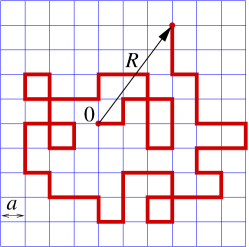
Figure 2: Random walk on a square lattice with elementary lattice step $a$. We choose each step at random. In two dimensions, two equivalent methods exist. In the first one, we draw heads or tails (with a probability of $1/2$) for a direction, vertical or horizontal, and next the orientation along the chosen direction. In the second method, we draw with the same probability (with probability of $1/4$) one of the four possible directions. In the continuous limit where the lattice step goes to 0, a very long random walk will take the appearance of the Brownian motion of figure 1.

The newness and the originality of Smoluchowski’s approach is in the replacement of an incredibly difficult problem (a Brownian particle which collides within a gas or liquid) by a relatively simple stochastic process. Each dynamic event like a collision is considered as a random event similar to a game of heads or tails, or to the throw of a dice, where the elementary probabilities are (to a certain extent) determined by underlying mechanical laws. This way of reasoning plays a fundamental role in mechanics and statistical physics today and, as Marc Kac noticed, it is difficult for us today to imagine the degree of Smoluchowski’s intellectual boldness in starting this subject during the early years of the last century.

1.5.3 Smoluchowski’s contributions

Smoluchowski knew about the most recent studies on Brownian motion and in particular the work of Felix Exner. The latter sent Smoluchowski diagrams made from memory, called “Krix-Krax” because of the several inter-crossing “jumps” apparently made by a Brownian particle observed under a microscope over a set of discrete instants of time.

Smoluchowski began by criticizing Nägeli’s arguments which claimed that a collision of a molecule of water with a sphere 0.001 mm in diameter would give a velocity of $3\times 10^{-6}$ cm/s, which would be impossible to observe under a microscope, and that the collision effects would cancel out on average. He compared this way of thinking to that of a player who believed himself never to be able to lose more than a single bet, despite repeated draws! By continuing the analogy further, he calculated for the heads or tails game how the positive (or negative) cumulated gains grow with the number $n$ of draws (“time”).

Let $p_{n,m}$ be the probability to have met $m$ favorable outcomes in the total of $n$ draws, with a net gain of $m-(n-m)=2m-n$. This probability can be written as

$$p_{n,m}=\frac{1}{2^{n}}\frac{n!}{m!(n-m)!}=\frac{1}{2^{n}}\left(n\atop m\right),$$ (45)

where the number of combinations $\left(n\atop m\right)$ is the number of ways of choosing $m$ out of $n$ objects.

The positive or negative mean deviation from zero, $\delta_{n}$, i.e., the average of the absolute value of a gain or of a loss after $n$ turns, can be calculated as

$$\delta_{n}=\langle|2m-n|\rangle=2\sum_{m={n}/{2}}^{n}(2m-n)p_{n,m}=2\sum_{m={n}/{2}}^{n}(2m-n)\frac{1}{2^{n}}\left(n\atop m\right)=\frac{n}{2^{n}}\left(n\atop{\frac{n}{2}}\right),$$

where $n$ is supposed an even number, to simplify the notation. For large $n$, we then use Stirling’s formula $n!\simeq n^{n}e^{-n}\sqrt{2\pi}$, to evaluate $\delta_{n}$:

$$\delta_{n}\simeq\sqrt{\frac{2n}{\pi}},\,\,\,n\gg 1.$$

The (arithmetical) average of successive gains (or losses) with respect to $0$ increases as $\sqrt{n}$, even when the total (algebraic) average is zero. The analogous number $n$ of molecular collisions per second on a sphere was estimated by Smoluchowski as $10^{16}$ in a gas and $10^{20}$ for a liquid. If the gain in velocity is of the order $10^{-6}$ cm/s at each collision, one obtains a mean cumulated velocity of from $10^{2}$ to $10^{4}$ cm/s per second. However Smoluchowski immediately reduces this conclusion, remarking that each individual gain of velocity will fluctuate, and that a high velocity value decreases the probability of one more positive gain.

He shows next that a “true” velocity could be obtained from the equipartition of kinetic energy, which gives a velocity of 0.4 cm/s, again much too large in relation to experimental observations! In fact, Exner’s diagrams in “Krix-Krax” gave a velocity of about $3\times 10^{-4}$ cm/s, an apparently irreconcilable disagreement. As Smoluchowski says, “this contradiction, already seen by F. Exner, seems at first to be a decisive objection to kinetic theory. Nevertheless the explanation is very simple.”

He presents the following simple and clear explanation: such a velocity is too large to be observed with a microscope magnifying 500 times. What one observes is the average position of a particle having this velocity, but hit $10^{20}$ times per second, each time in a different direction, such that one cannot observe the instantaneous velocity. Each zig-zag displacement is incomparably smaller than the particle’s size, and it is only when the geometric sum of these elements reaches a certain value that one can observe a displacement. This is clearly the substance of Einstein’s argument, here supported by the concrete image of kinetic theory: the average displacement is the observable physical quantity, while velocity is not.

After such qualitative, but illuminating, considerations, Smoluchowski develops his model of random collisions. Let $m$ and $v$ ($m^{\prime}$ and $v^{\prime}$ respectively) be the mass and the velocity of a particle in suspension (of molecules in the liquid, respectively). From the equipartition of energy, one has on average:

$$\frac{v}{v^{\prime}}=\sqrt{\frac{m^{\prime}}{m}}.$$ (46)

He affirms that from “the laws of collision of elastic spheres,” the change of velocity of the sphere in suspension is, at a collision, on average given by a small transverse component $\alpha\,m^{\prime}v^{\prime}/m$, where $\alpha=3/4$. The result is a random change of the velocity direction of a small angle $\varepsilon=\alpha\,m^{\prime}v^{\prime}/mv$. (According to (46), one also has $\varepsilon=\alpha v/v^{\prime}$ on average.) He assumes also that the molecular impacts occur after equal intervals of time, which makes the particle trajectory a chain made of constant-length segments.

In other words, Smoluchowski adapts the idea of the mean free path of a molecule in a gas, even though here the persistence of motion is shortened by the presence of numerous molecules of the surrounding fluid.

The problem of Brownian motion is thus mathematically mapped onto the one of finding the end-to-end average distance $\Delta_{n}^{2}$, of a chain of $n$ segments, all of length $\ell$, each randomly turned by a small angle $\varepsilon$ with respect to the preceding one. He then obtains the general solution by a complicated recurrence relation, containing multiple angular integrals of trigonometric functions, of the form:

$$\Delta_{n}^{2}=\ell^{2}\left\{\frac{2n}{\delta}+1-n-2\frac{(1-\delta)^{2}-(1-\delta)^{n+2}}{\delta^{2}}\right\},$$ (47)

where $\delta=1-\cos\varepsilon\simeq\varepsilon^{2}/2$.

In the limit where $n\delta$ is small, one finds

$$\Delta_{n}=n\ell\left(1-\frac{n\delta}{6}\right),$$ (48)

which represents a quasi-ballistic trajectory.

In the opposite case of a large number of collisions per unit of time $n\delta\gg 1$ , the first term of (47) dominates and one finds the expected result:

$$\Delta_{n}^{2}=\ell^{2}\frac{2n}{\delta}=\ell^{2}\frac{4n}{\varepsilon^{2}}.$$ (49)

If we call $\bar{n}$ the number of collisions per unit of time, such that there are $n=\bar{n}\,t$ collisions over the time $t$, we have for a free path $\ell=v/\bar{n}$, and by using $\varepsilon=\alpha v/v^{\prime}$, we find an average quadratic displacement at time $t$,

$$\Delta_{n}^{2}\equiv\Delta_{t}^{2}=\frac{4}{\alpha^{2}}\frac{v^{\prime\,2}}{{\bar{n}}}{t}.$$ (50)

The momentum $mv$ of the particle in suspension changes on average by a quantity $\alpha^{\prime}m^{\prime}v$ per collision, where, from Smoluchowski, $\alpha^{\prime}=2/3$, which means the friction force $F=-\bar{n}\alpha^{\prime}m^{\prime}v$, and thus the friction coefficient $\mu=\bar{n}\alpha^{\prime}m^{\prime}$. Substituting $\mu$ in $\bar{n}$ one obtains: $\Delta_{t}^{2}=\frac{4{\alpha^{\prime}}}{\alpha^{2}}\frac{{m^{\prime}}v^{\prime\,2}}{{\mu}}{t}.$ From the equipartition of kinetic energy of the molecules in the surrounding fluid: $\langle{m^{\prime}}{v^{\prime\,2}}\rangle=3RT/\mathcal{N}$, and the result of Smoluchowski finally becomes:

$$\Delta_{t}^{2}=\frac{2\alpha^{\prime}}{\alpha^{2}}\,6\frac{RT}{{\mu}\mathcal{N}}{t}.$$ (51)

One finds again the Sutherland-Einstein result (15), (28), this time in three dimensions, with a supplementary numerical factor of kinetic origin $2\alpha^{\prime}/{\alpha^{2}}=(4/3)^{3}=64/27$. Because of the various physical and geometrical approximations involved, this factor should perhaps not come as a surprise! The experiments of The (Theodor) Svedberg in 1907 seemed to support this result, but Langevin mentioned later in 1908, in his article in the Comptes Rendus, that once these approximations were corrected, Smoluchowski’s stochastic method gave the same formula (28) as Einstein’s method. Smoluchowski himself adopted this formula in his subsequent articles.

Afterwards he gave the complete theory of density fluctuations within an ensemble of Brownian particles, as well as that of their sedimentation in a gravitational field and of the coagulation of colloids. The content of this reference is described in detail by S. Chandrasekhar in his famous review article on Stochastic Problems in Physics and Astronomy and praised as follows:

“In [this] reference […] we have an extremely valuable account of the entire subject of Brownian motion and molecular fluctuations; there exists no better introduction to this subject than these lectures by Smoluchowski.”

He adds: “The theory of density fluctuations as developed by Smoluchowski represents one of the most outstanding achievements in molecular physics. Not only does it quantitatively account for and clarify a wide range of physical and physico-chemical phenomena, it also introduces such fundamental notions as the ‘probability after-effect’ which are of great significance in other connections.”

We should also mention that we owe to Smoluchowski (and to Einstein) the theory of critical opalescence as well.

Smoluchowski’s name is traditionally attached to the generalization of the diffusion equation (16) governing the probability density $P(\vec{r},t)$ in presence of a force field $\vec{F}(\vec{r})$:

$$\frac{\partial P}{\partial t}=D\Delta_{\vec{r}}P-\frac{1}{\mu}{\rm div}_{\vec{r}}(\vec{F}P),$$ (52)

where $\mu$ is the same as in (14). This equation applies directly to the case of a uniform gravitational field. In one dimension it is simply written as

$$\frac{\partial P(x,t)}{\partial t}=D\frac{\partial^{2}}{\partial x^{2}}P(x,t)+\frac{1}{\mu}\frac{\partial}{\partial x}\left(\frac{\partial V(x)}{\partial x}P(x,t)\right),$$ (53)

for a force field $F(x)$ derived from a potential $V(x)$.

The passage to such a differential equation in configuration space was first achieved by Smoluchowski in 1915. This equation, as the standard “free field” diffusion equation, are valid only if we ignore effects which happen in time intervals of the order of the viscous damping time, $\tau=m/\mu$, introduced in eq. (43).

When such effects are of interest, as in eq. (42), one should use a more general differential equation, the so-called Fokker-Planck equation. The passage to such a differential equation for the description in velocity space of the Brownian motion of a free particle was indeed achieved by Fokker, while a more general discussion of this problem is due to Planck. Let us also mention the pionnering work by Rayleigh in one dimension as early as 1891!

The Fokker-Planck equation is a differential equation governing the time evolution of the probability density $\mathcal{P}(\vec{p},t)$ in velocity ($\vec{v}$) or momentum ($\vec{p}=m\vec{v}$) space, valid for all time intervals. In the absence of an external force field, it has the form

$$\frac{\partial\mathcal{P}}{\partial t}={\mu^{2}}D\Delta_{\vec{p}}\mathcal{P}+{\mu}\,{\rm div}_{\vec{p}}\left(\frac{\vec{p}}{m}\mathcal{P}\right).$$ (54)

This is fully equivalent to the description of Brownian motion by the stochastic Langevin equation, described in $\mathbb{S}$ 1.7.1 below.

Their solution gives the full Ornstein-Uhlenbeck process. For times shorter than the damping time $\tau$, a ballistic regime dominates, while asymptotically one recovers the so-called “overdamped” regime, i.e., standard diffusion. [See eqs. (42-44) and $\mathbb{S}$ 1.7.3.]

When an external force field is present, a more general probabilistic description in phase space, involving the probability density function $\mathbb{P}(\vec{p},\vec{r},t)$ for both the momentum $\vec{p}$ and the position $\vec{r}$ of the Brownian particle, is required. Its time evolution, valid for all time intervals, is then given by

$$\frac{\partial\mathbb{P}}{\partial t}+\frac{\vec{p}}{m}\cdot\vec{\nabla}_{\vec{r}}{\mathbb{P}}+\vec{F}\cdot\vec{\nabla}_{\vec{p}}{\mathbb{P}}={\mu^{2}}D\Delta_{\vec{p}}\mathbb{P}+{\mu}\,{\rm div}_{\vec{p}}\left(\frac{\vec{p}}{m}\mathbb{P}\right).$$ (55)

The foregoing equation represents the complete generalization of the Fokker-Planck equation (54) to the phase space. At the same time eq. (55) represents also the generalization of Liouville’s equation of classical mechanics to include Brownian motion; more particularly, on the right-hand side of eq. (55) we have the terms arising from Brownian motion while on the left-hand side we have the usual Stokes differential operator $D/Dt$ acting on $\mathbb{P}$.

The earliest attempts to generalize Liouville’s equation of classical mechanics to include Brownian motion were made by O. Klein and H. A. Kramers, culminating with the work by S. Chandrasekhar.

1.5.4 Brownian motion and the second principle

Another aspect of Smoluchowski’s work concerns the correct statistical formulation of the second principle of thermodynamics. With The Svedberg’s recent data on Brownian motion, Smoluchowski had experimental results which permitted him, armed with his own theory of fluctuations near-to-equilibrium, to estimate the persistence and recurrence times of a system slightly out of equilibrium, and to check these results against experiments. He used neither phase space, nor Liouville’s theorem as in classical statistical mechanics à la Boltzmann. He introduced simply the calculus of probability. By incorporating the theory of fluctuations he gave a correct formulation of the second principle of thermodynamics, where this principle appeared valid only in a statistical sense, and was therefore susceptible to multiple twists at the microscopic level. These considerations are relevant to and bear on Loschmidt’s reversibility paradox and Zermelo’s recurrence paradox. Discussing these paradoxes in the context of Boltzmann’s views, Smoluchowski concludes that “a process appears irreversible if the initial state is characterized by a long average time of recurrence compared to the times during which the system is under observation.”

Further precision experiments carried out with expressed intention of verifying Smoluchowski’s theory are those of A. Westgren, as described in the survey article by S. Chandrasekhar.

A modern discussion of Smoluchowski’s ideas was given by Richard Feynman in his famous elementary physics lectures. He compared Maxwell’s demon with a ratchet and pawl and an electric rectifier, neither of which can systematically transform internal energy from a single reservoir to work. He wrote:

“If we assume that the specific heat of the demon is not infinite, it must heat up. It has but a finite number of internal gears and wheels, so it cannot get rid of the extra heat that it gets from observing the molecules. Soon it is shaking from Brownian motion so much that it cannot tell whether it is coming or going, much less whether the molecules are coming or going, so it does not work.”

Modern day computer simulations strikingly reveal the fluctuation phenomena envisaged by Smoluchowski and Feynman.

Smoluchowski’s observation suggested that Maxwell’s demon ought to be buried and forgotten. But that did not happen, apparently because Smoluchowski’s approach left open the possibility that somehow, a perpetual motion machine operated by an “intelligent” being might be achievable. It was this fascinating idea of using intelligence that captured Leo Szilard’s interest, in his classic 1929 paper, “On the decrease of entropy in a thermodynamic system by the intervention of intelligent beings.”

The feature associated with intelligence that is needed by a demon is memory: it must remember what it measures, even if only briefly. Notably, Szilard discovered with his heat engine, with a one-molecule working fluid, the idea of a “bit” of information with entropy $k_{B}\ln 2$, now central in computer science, and established the connection between entropy and information.

At this stage, rather than fully opening Pandora’s box which contains the Protean Maxwell’s demons, we prefer to recommend the survey, Maxwell’s Demon 2, by H. S. Leff and A. F. Rex and in particular the thoughtful introduction of the second edition. Let us only mention a few historical landmarks that are described in their presentation.

After a hiatus of 20 years, Léon Brillouin, assuming the use of (quantum) light signals in the demon’s attempts to defeat the second law, concluded that information acquisition, like measurement, is dissipative. This led him to break new ground by developing an extensive mathematical theory connecting measurement and information. The impact of Brillouin’s and Szilard’s work was far reaching and the result was a proclaimed, but temporary, “exorcism” of the demon.

A new life began for the demon when Rolf Landauer made the important discovery that memory erasure in computers feeds entropy to the environment. This is now called “Landauer’s principle”. It states that the erasure of one bit of information stored in a memory device requires sending an amount of entropy of at least $k_{B}\ln 2$ to the environment, i. e., a minimal heat generation of $k_{B}T\ln 2$.

Charles Bennett, after his important demonstration in 1973 that reversible computation, which avoids the erasure of information, is possible in principle, argued in 1982 that erasure of a demon’s memory is the fundamental act that saves the second law because of Landauer’s principle. This was a turning point in the history of Maxwell’s demon.

In his 1970 book Foundations of Statistical Mechanics, Oliver Penrose independently recognized the importance of “resetting” operations that bring all members of a statistical ensemble to the same observational state. Applied to Szilard’s heat engine, this is nothing else than memory erasure, which sends an amount of entropy of at least $k_{B}\ln 2$ to the environment.

Among recent proofs of Landauer’s principle we cite here, somehow arbitrarily, the one by K. Shizume, who uses a solvable model of memory based on a Brownian particle in a time-dependent potential well; the one by M. Magnasco with a detailed analysis of Szilard’s heat engine; and the one by B. Piechocinska, who assumes the decoherence of the states of the thermal reservoir.

Let us finally mention that, despite several attempts to argue against its validity, the Landauer-Penrose-Bennett framework seems to be generally accepted as providing the solution to the Maxwell’s demon–second principle puzzle, at least in classical mechanics, and in a thermodynamical limit of some sort.

However, there are now indications that Landauer’s principle, as well as the second principle, might not hold in the (strong) quantum regime. The source of the violation is quantum entanglement between the system and the constant-temperature reservoir, which then act as a single entity.

In close relation to Brownian motion and the second principle, the topic of Brownian motors has recently received considerable attention. C. Van den Broeck et al. were able to find a solvable model for a thermal Brownian motor. They show that immersed in two different thermal baths, two rigidly coupled Brownian particles with a geometrical asymmetry can function as a microscopic engine able to rectify Brownian fluctuations. As expected, when the temperatures of the two baths are equal, the drift motion ceases, and one is left only with a standard Brownian displacement, which obeys Gauss’ distribution law. The drift speed can be computed exactly for convex bodies, in the limit of dilute gases. Extremely precise molecular dynamics simulations with hard disks confirm the theory. In effect, this is a microscopic and soluble Feynman’s ratchet.

In a recent work, Van den Broeck and Kawai propose a model for a Brownian refrigerator, with a cooling mechanism based on such a Brownian motor submitted to an external force. A heat flow is generated between the two components of the motor. Such a marvellously simple microscopic model would have certainly greatly pleased Einstein, Smoluchowski and Sutherland!

It is necessary to note here that these discussions are current research topics of intense interest. In fact today there exist new theoretical results, known as the Gallavotti-Cohen fluctuation theorem, Jarzynski’s equality, or Crooks’ fluctuation theorem. They quantify the spontaneous average work provided by a source of heat during irreversible phenomena. The manipulations of single biological molecules like DNA and RNA, which are mesoscopic objects, allow the experimental testing of these relations. The interpretations of these results and experiments are currently the topic of a lively debate, just as at the dawn of Brownian motion!

1.5.5 Brownian motion and the mathematical aspects of irreversibility

Let us open here a brief mathematical parenthesis. Einstein’s and Smoluchowski’s theories, based upon a Newtonian dynamics of the particles, in fact postulated the emergence of Brownian motion from a classical non-dissipative reversible dynamics, a point of view which was far from being physically obvious or, a fortiori, mathematically rigorous. This led to the heated controversy about the second principle. The key difficulty is similar to the justification of Boltzmann’s molecular chaos assumption (“Stosszahlansatz”) standing behind the derivation of the Boltzmann equation. Mathematically, the dissipative character can only emerge in a scaling limit, as the number of degrees of freedom goes to infinity.

As we shall see below, the first mathematical definition of Brownian motion was given only in 1923 by Wiener. But the derivation of Brownian motion from Hamiltonian dynamics was not seriously investigated until the end of the seventies. Kesten and Papanicolaou proved that the velocity distribution of a particle moving in a random scatterer environment (the so-called Lorenz gas with random scatterers) converges to Brownian motion in dimension $d\geq 3$. The same result was obtained in $d=2$ dimensions by Dürr, Goldstein and Lebowitz. A very recent work establishes the convergence to Brownian motion in position space as well.

Bunimovich and Sinai proved the convergence to Brownian motion of the periodic Lorenz gas with a hard-core interaction. The only source of randomness there is the distribution of the initial conditions. Finally, Dürr, Goldstein and Lebowitz established rigorously that the velocity process of a heavy particle in an ideal gas converges in three (actually an arbitrary number of) dimensions to the Ornstein-Uhlenbeck process, that is the version of Brownian motion described by Langevin’s equation (see below). The same result in one dimension was first established by R. Holley.

Brownian motion was discovered and theorized in the context of classical mechanics, and it postulates a microscopic reversible Newtonian world for atoms and molecules. Nowadays, it is thus natural to replace Newtonian dynamics with Schrödinger dynamics and investigate if Brownian motion still correctly describes the motion of a quantum particle in a random environment. For a discussion of this fundamental and difficult question, we refer the reader to a recent work by Erdös, Salmhofer and Yau and to the references therein.

1.5.6 Smoluchowski’s legacy

With Einstein, Smoluchowski shares the credit for having shown the importance of microscopic fluctuations in statistical physics, at the same time promoting the probabilistic approach. In this sense he appears as a great master inheritor in physics of the Doctrine of Chance of Abraham de Moivre.

In 1917, Marian von Smoluchowski had just been elected rector of the Jagellonian University in Kraków (Cracow) University, but he was never to fulfill his new task. During the summer he succumbed to an epidemic of dysentery. During his illness he complained to his wife that he could have done so much more. He died prematurely in September of 1917 at the age of forty five.

In 1973 Chandrasekhar was awarded the Marian von Smoluchowski Medal of the Polish Physical Society in appreciation of his contributions to stochastic methods in physics and astrophysics and, especially, the Review of Modern Physics 1943 article which covered Smoluchowski’s contributions. In his speech at the award ceremony, Chandrasekhar noted that the Nobel prizes in chemistry awarded to R. Zsigmondy in 1925 and to T. Svedberg in 1926 were for experimental confirmation of Smoluchowski’s theoretical predictions on colloidal and disperse systems and that if Smoluchowski had been still alive he would certainly have been a Nobel laureate himself.

1.6 Louis Bachelier

1.6.1 Bachelier and mathematical finance

Louis Bachelier is nowadays considered as having laid the foundations for mathematical finance, and is further credited with the first mathematical study of the continuous Brownian process, including a random walk approach to the latter. A detailed and very interesting presentation of Bachelier’s life and scientific achievements was given in 2000 in an essay, entitled Louis Bachelier on the Centenary of Théorie de la Spéculation, for the centenary of the publication of his thesis. This section is essentially based on this presentation, and a significant part of it incorporates material in the cited article.

The importance of Bachelier’s work was not properly recognized during his time. As Benoît Mandelbrot writes in The Fractal Geometry of Nature, it was Kolmogorov in 1931 who re-discovered his name in an article in Mathematische Annalen.

Bachelier was interested in the theory of speculation at the Paris stock market. He successfully defended his thesis, entitled Théorie de la spéculation, on 29 March 1900 at the Sorbonne, in front of a jury composed of Paul Appell, Joseph Boussinesq and Henri Poincaré, his thesis advisor. As a work of exceptional merit, stongly supported by Poincaré, his thesis was published in the Annales Scientifiques de l’École Normale Supérieure.

1.6.2 The Thesis

Bachelier begins with the mathematical modeling of stock price movements, and formulates the principle that “the expectation of the speculator is zero,” by which he means that the conditional expectation given the past information is zero. In other words, he assumes that the market evaluates assets according to a martingale measure. The further hypothesis is that the price evolves as a continuous Markov process (with no memory), homogeneous in time and space. Bachelier then shows that the density of one-dimensional distributions of this process satisfies an integral relation, now known as the Chapman-Kolmogorov equation. Bachelier, without addressing the question of uniqueness, shows that the Gaussian density, with a linearly increasing variance, solves this equation.

He also considers a discrete version of the problem, where the price process is the continuum limit of random walks, and where the binomial formula (45) appears. He then proceeds to show that the distribution functions of the process satisfy Fourier’s heat equation, as in the similar eq. (22) in Einstein’s article. Bachelier then introduces a novel expression: “the radiation of the probability”.

One finds indeed many of the well-known results for Brownian motion: On p. 37 of his memoir, one reads that: “On voit que la probabilité est régie par la loi de Gauss déjà célèbre dans le Calcul des probabilités;” on p. 38, that “ L’espérance mathématique

$$\int_{0}^{\infty}pxdx=k\sqrt{t}$$

est proportionnelle à la racine carrée du temps.” Bachelier also calculates the probability that the Brownian motion does not exceed a fixed level and finds the distribution of the supremum of that motion.

He therefore developed in his first thesis a theory of continuous stochastic processes close to the modern mathematical theory of Brownian motion. As stressed by the authors of the essay Louis Bachelier on the Centenary of Théorie de la Spéculation, “more than one hundred years after the publication of the thesis, it is quite easy to appreciate the importance of Bachelier’s ideas. The thesis can be viewed as the origin of mathematical finance, and of several branches of stochastic calculus such as the theory of Brownian motion, Markov processes, diffusion processes, and even weak convergence in functional spaces.”

It is also quite interesting to read Poincaré’s original report, translated in the essay cited above. Poincaré’s report shows that Bachelier’s thesis was highly appreciated by the outstanding mathematician. In contrast to the legend that the evaluation note “honorable” means somehow that the examiners were dissatisfied with the thesis, it can perhaps be argued that it might have been the highest grade possible for a thesis which was addressing a problem not in the realm of standard mathematics, and that in addition had a number of non-rigorous arguments.

The official report of the Thesis Committee states:

In the presentation of his First Thesis, M. Bachelier showed mathematical intelligence and insight. He has added some interesting results to those already contained in the printed version of the thesis, in particular an application of the image method.

As for the Second Thesis, he proved to possess a complete knowledge of Boussinesq’s work on the motion of a sphere in an indefinite fluid.

The Faculty gave him the degree of Doctor with honors.

Paul Appell, President

It is indeed very intriguing that the “Proposal given by the Faculty,” subject of his Second Thesis, was entitled: Resistance of an indefinite liquid mass with internal frictions, described by the formulae of Navier, to small translational motions of a solid sphere, submerged inside the fluid and adhering to it.

But there is of course no mention in his first thesis, published in 1900, about any link between the speculation problem and the motion of a sphere in a viscous fluid! However, we saw above Poincaré’s early interest in Brownian motion in relation to Carnot’s principle. We also saw that Einstein’s (as well as Sutherland’s) application of hydrodynamical laws to the motion of a sphere suspended in a fluid, was key to the solution of Brownian motion. We now observe the amazing coincidence that the thesis subject proposed by the Faculty, if joined with the subject of the first thesis, could have led Poincaré and Bachelier to establish the quantitative theory of Brownian motion, before any of Einstein, Sutherland or Smoluchowski! All necessary mathematical equations were indeed present for that, if only a little spark of physical intuition would have struck these eminent mathematicians!

1.6.3 Further Studies

Louis Bachelier continued to develop the mathematical theory of diffusion processes in a series of memoirs and books. In his 1906 memoir on the Théorie des probabilités continues, he defined new classes of stochastic processes, which are now called processes with independent increments and Markov processes, and he derived the distribution of the Ornstein-Uhlenbeck process.

He was aware of the importance of his contributions. He wrote in his 1924 “Notice de Travaux” that “this theory has no relation to the geometrical theory of probability, the range of application of which is quite limited. We are concerned here with a science of a different order of generality, compared to classical probability calculus. Among the new concepts, one can cite the assimilation to an energy of the probability which is an abstraction. That original concept was noticed by Henri Poincaré, and it made much progress possible.” One also reads about his 1912 book Calcul des probabilités, that “it is the first that surpassed the great treatise by Laplace.”

We shall not describe in detail here the very unfortunate misunderstanding with Paul Lévy, which in 1926 prevented Bachelier from becoming a full professor at the University of Dijon. We refer the interested reader to the essay mentioned above for a thorough and well-documented analysis of this dramatic event.

Later, Lévy, under the influence of Kolmogorov’s fundamental paper (1931) on diffusion processes, which referred to Bachelier’s work, realized that a number of properties of Brownian motion had been discovered by Bachelier several decades earlier. He revised his opinion, and wrote him a letter with apologies.

Bachelier’s ideas receive nowadays a widespread recognition. Famous probability treatises, like the ones by W. Feller, An Introduction to Probability Theory and its Applications (1957), or by K. Itô and H. McKean, Diffusion Processes and their Sample Paths (1965), refer to Bachelier’s seminal work.

In the literature written by economists, one finds reference to him in Keynes (1921), and more recently in the work of other famous economists, like that of the 1997 Nobel laureates in Economic Sciences, Robert Merton and Myron Scholes. It is perhaps appropriate here to reproduce Merton’s tribute to Bachelier:

“ The origin of much of the mathematics in modern finance can be traced to Louis Bachelier’s 1900 dissertation on the theory of speculation, framed as an option-pricing problem. This work marks the twin births of both the continuous-time mathematics of stochastic processes and the continuous-time economics of derivative-security pricing.”

No doubt that today Bachelier would have been awarded a Nobel Prize in Economic Sciences for his work of 1900!

1.7 Paul Langevin

Knowing the great interest in the theory of Brownian motion, signalled by the works of Gouy, Einstein, and Smoluchowski, Langevin took the next steps in 1908. He first said that the factor of 64/27 of Smoluchowski’s results, due to the approximations made, was erroneous and that the result coincided with Einstein’s formula (28) after his correction. Next, he provided another demonstration of this fact, in which was contained the first mathematical example of a stochastic equation.

1.7.1 Langevin’s equation

Langevin’s argument is enlightening and we follow his demonstration faithfully. The starting point is the Maxwell equipartition theorem of kinetic energy. It states that the energy of a particle in suspension inside a fluid in thermal equilibrium has, for instance in the $x$ direction, an average kinetic energy $\frac{1}{2}\frac{RT}{\mathcal{N}}$, equal to that of any gas molecule, in a given direction, at the same temperature. This is directly related to van ’t Hoff’s law seen above, which affirms the identity between diluted solutions and perfect gases. If $v=\frac{{\rm d}x}{{\rm d}t}$ is the particle velocity in a chosen direction at a given moment, then the average over a large number of identical particles with mass $m$ is

$$\frac{1}{2}m\langle v^{2}\rangle=\frac{1}{2}\frac{RT}{\mathcal{N}}.$$ (56)

A particle which is large compared to the molecules of a liquid, and is moving at speed $v$ with respect to this liquid, experiences a viscous resistance force equal to $-6\pi\eta av$, according to Stokes’ formula. In reality this is only an average value, and because of the irregular shocks of the surrounding molecules, the action of the fluid on the particle fluctuates around the average value. The equation of motion along the direction $x$, given by Newtonian dynamics, is

$$m\frac{{\rm d}v}{{\rm d}t}=m\frac{{\rm d^{2}}x}{{\rm d}t^{2}}=-6\pi\eta av+X.$$ (57)

The complementary force $X$, introduced by Langevin, is random, and also called stochastic. In reality we know little about it, apart from that it is equally likely to be positive or negative, and that its magnitude is such that it maintains the particle’s agitation which, without it, would end by stopping because of the viscous resistance.

By multiplying equation (57) by $x$, one has

$$mx\frac{{\rm d}v}{{\rm d}t} = \frac{1}{2}m\frac{{\rm d^{2}}x^{2}}{{\rm d}t^{2}}-mv^{2}$$ (58)

$$= -\mu\,xv+xX=-\mu\frac{1}{2}\frac{{\rm d}x^{2}}{{\rm d}t}+xX,$$

where the friction coefficient $\mu$ represents $\mu=6\pi\eta a$ as before. If we consider a large number of identical particles and take the average of equations (58) written for each of them, then the average value of the term $xX$ is “evidently” zero because of the irregularity of the random forces $X$, and one finds

$$\frac{1}{2}m\frac{{\rm d^{2}}\langle x^{2}\rangle}{{\rm d}t^{2}}-m\langle v^{2}\rangle=-\mu\frac{1}{2}\frac{{\rm d}\langle x^{2}\rangle}{{\rm d}t}.$$ (59)

One puts $u=\frac{1}{2}\frac{{\rm d}\langle x^{2}\rangle}{{\rm d}t}$, and uses the equipartition theorem of kinetic energy (56) to get a simple differential equation of first order:

$$m\frac{{\rm d}u}{{\rm d}t}-\frac{RT}{\mathcal{N}}=-\mu u.$$ (60)

The general solution is

$$u=\frac{RT}{\mu{\mathcal{N}}}+C\exp\left(-\frac{\mu}{m}t\right),$$ (61)

where $C$ is an arbitrary constant. The exponentially decreasing term rapidly fades away, and the result goes to the constant value of the first term, in a limiting regime after a time $\tau$ of order $\frac{m}{\mu}$ or $10^{-8}$ seconds, for all Brownian particles.

Thus, we have

$$u=\frac{1}{2}\frac{{\rm d}\langle x^{2}\rangle}{{\rm d}t}=\frac{RT}{\mu\mathcal{N}},$$ (62)

from which, for the time interval $t$,

$$\langle x^{2}\rangle=\frac{2RT}{\mu\mathcal{N}}t=\frac{RT}{\mathcal{N}}\frac{1}{3\pi\eta a}t,$$ (63)

if one supposes that the particle was observed at the origin $x=0$ at time $t=0$. Langevin’s method indeed reproduces Einstein’s result (28). In this paper (published in 1908 in the Comptes Rendus of the Academie de Sciences) Langevin introduced, without knowing it, the first element (the random force $X$) of what was to become stochastic calculus.

1.7.2 Boltzmann’s constant

Boltzmann’s constant $k_{B}$ is obtained by dividing the molar constant $R$ of a perfect gas by Avogadro’s number $\mathcal{N}$, such that one obtains a quantity which refers to a single molecule:

$$k_{B}=\frac{R}{\mathcal{N}}=1.381\times 10^{-23}\,{\rm J}\,{\rm K}^{-1}.$$ (64)

The energy $k_{B}T$ gives the average thermal energy at the standard temperature: $k_{B}T=4\times 10^{-21}$ J. The constant $k_{B}$ was not introduced by Boltzmann but by Planck in his famous presentation on December 14, 1900, on black-body radiation, at the same time he presented Planck’s constant $h$!

1.7.3 An analysis of the solution of Langevin’s equation.

The method presented in section (1.7.1) is the one that Langevin gave in his original paper. A more modern formulation proceeds from the time-correlation functions of the stochastic force $X$ in canonical form,

$$\langle X\rangle={0},\,\,\langle X(t)X(t^{\prime})\rangle=A\delta(t-t^{\prime}),$$ (65)

where $A$ is a coefficient to be determined and $\delta(t-t^{\prime})$ is the Dirac distribution. The generalization to $d$ dimensions is

$$\langle\vec{X}\rangle = \vec{0},$$

$$\langle X_{i}(t)X_{j}(t^{\prime})\rangle = A\delta_{ij}\delta(t-t^{\prime}),$$ (66)

where $\delta_{ij}$ is the Kronecker symbol and $i,j=1,\cdots d.$

We can easily integrate the linear equation for the velocity

$$m\frac{{\rm d}{\vec{v}}}{{\rm d}t}=-\mu{\vec{v}}+\vec{X}.$$ (67)

The solution is

$${\vec{v}}(t)={\vec{v}}(0)\,e^{-\frac{\mu}{m}t}+\frac{1}{m}\int_{0}^{t}{\rm d}t^{\prime}\,\vec{X}(t^{\prime})\,e^{-\frac{\mu}{m}(t-t^{\prime})}.$$ (68)

Therefore by taking the square of the velocity and by using formula (66), we find the average value of kinetic energy at time $t$

$$\frac{1}{2}m\langle{\vec{v}}^{\,2}(t)\rangle=\frac{Ad}{4\mu}\left(1-e^{-2\frac{\mu}{m}t}\right)+\frac{1}{2}m{\vec{v}}^{\,2}(0)e^{-2\frac{\mu}{m}t}.$$ (69)

We then see that this energy relaxes towards a constant value at large time, i.e., at equilibrium. From the theorem of equipartition of kinetic energy,

$$\frac{1}{2}m\langle{\vec{v}}^{\,2}(t)\rangle_{t\to\infty}=\frac{d}{2}k_{B}T,$$ (70)

we deduce the important identity

$$A={2}\mu k_{B}T.$$ (71)

We then have

$$\langle{\vec{v}}^{\,2}(t)\rangle=\frac{dk_{B}T}{m}+\left({\vec{v}}^{\,2}(0)-\frac{dk_{B}T}{m}\right)e^{-2\frac{\mu}{m}t}.$$ (72)

A second stage consists in integrating equation (68) to obtain the displacement $\vec{r}(t)-\vec{r}(0)$. Then taking the square, and the stochastic average by means of formulae (66), we obtain after some calculation,

$$\langle\left[\vec{r}(t)-\vec{r}(0)\right]^{2}\rangle = 2dD\left[t-\frac{m}{\mu}\left(1-e^{-\frac{\mu}{m}t}\right)\right]$$ (73)

$$+ \left({\vec{v}}^{\,2}(0)-\frac{dk_{B}T}{m}\right)\left(\frac{m}{\mu}\right)^{2}\left(1-e^{-\frac{\mu}{m}t}\right)^{2},$$

where $D=k_{B}T/\mu$, as before. The derivative $u$ considered by Langevin is then given by

$$u = \frac{1}{2}\frac{{\rm d}}{{\rm d}t}\langle\left[\vec{r}(t)-\vec{r}(0)\right]^{2}\rangle$$ (74)

$$= d\frac{k_{B}T}{\mu}-{\vec{v}}^{\,2}(0)\frac{m}{\mu}e^{-\frac{\mu}{m}t}+\left({\vec{v}}^{\,2}(0)-\frac{dk_{B}T}{m}\right)\frac{m}{\mu}e^{-2\frac{\mu}{m}t}.$$

Notice first that these results at large $t$, or $t\gg\tau=m/\mu$, go asymptotically to those of thermal equilibrium and to the associated motion of diffusion, as expected. One remarks then the role played by the initial velocity in memory effects and in the approach to equilibrium. A very special value of ${\vec{v}}^{\,2}(0)$ is that of equipartition $\frac{dk_{B}T}{m}$. For this value only, the average quadratic velocity in (72) becomes invariant in time, $\langle{\vec{v}}^{\,2}(t)\rangle=\frac{dk_{B}T}{m},\forall t$. The average quadratic displacement (73) then takes Ornstein’s simple form (42), and the quantity $u$ (74) takes the form predicted by Langevin in (61), with a determined value for $C$. One consistently obtains the same result by using for ${\vec{v}}^{\,2}(0)$ its most probable value, meaning its thermal average at equipartition. One can then understand (but only a posteriori) the consistency of Langevin’s approach when he inserted the identity (56) in the middle of the derivation. That amounted to chosing the peculiar boundary condition ${\vec{v}}^{\,2}(0)=\frac{dk_{B}T}{m}$, which enforces stationary equipartition!

On the other hand, if one gives to the initial quadratic velocity ${\vec{v}}^{\,2}(0)$ a value which is different from that of equilibrium, the relaxation will occur in a bit more complex way, as we showed in the above results.

The regime at short times, $\frac{m}{\mu}\gg t$, also naturally depends on the initial conditions. In fact, by developing in series (73) one finds the expected ballistic regime

$$\langle\left[\vec{r}(t)-\vec{r}(0)\right]^{2}\rangle={\vec{v}}^{\,2}(0)\,t^{2}+{\mathcal{O}}(t^{3}),$$

that naturally cross-checks with (44) if one takes once again the value at equipartition.

1.7.4 Microscopic model

The force proposed by Langevin, $-\mu v+X$, can only be an approximation to the underlying molecular reality, made up of innumerable collisions where multiple correlations, due to interactions between molecules, exist at very short time scales. The stochastic term $X$ in (65,66) is a white noise without memory, i.e., it neglects temporal correlations.

Moreover, the hydrodynamic form of the friction term, $-\mu v$, is a description that pertains to the continuous limit, which requires extremely frequent collisions of the particle in suspension. The mass $m$ of the particle must then be large enough so that the characteristic time $\tau=m/\mu$ is large compared to the inverse frequency of collisions.

To give an idea of the origin of Langevin’s equation (57) and of its parameters $\mu$ and $A$ (71), it is natural to consider the simplest model, where the collisions of a particle in suspension occur with a surrounding perfect gas, and thus itself without interaction.

One can therefore consider a perfect gas of identical particles with mass $m^{\prime}$, a particle density $n^{\prime}$, at temperature $T$, and colliding the particle of large mass $m$ in suspension. To simplify, we consider the gas in one dimension, where the equations for the particle-gas elastic collisions are particularly simple. One then finds that the equation for the momentum variation of the test particle is similar to Langevin’s equation, with the explicit coefficients

$$\mu=4n^{\prime}\sqrt{\frac{2m^{\prime}k_{B}T}{\pi}},\,\,\,\,A=8n^{\prime}k_{B}T\sqrt{\frac{2m^{\prime}k_{B}T}{\pi}};$$ (75)

$\mu$ and $A$ thus verify (71).

It is then particularly interesting to rewrite these terms as a function of molar sizes that characterize the perfect gas. One introduces as well the gas pressure $p^{\prime}$, which responds to the equation of perfect gases $p^{\prime}=n^{\prime}k_{B}T$, which gives

$$\mu=4p^{\prime}\sqrt{\frac{2\mathcal{M}}{\pi RT}},\,\,\,\,A=\frac{2RT}{\mathcal{N}}4p^{\prime}\sqrt{\frac{2\mathcal{M}}{\pi RT}},$$ (76)

where $\mathcal{M}=\mathcal{N}m^{\prime}$ is the molar mass of the gas.

A similar problem can be solved in three dimensions. The friction coefficient $\mu$ and Brownian coefficient $A$ are in this case

$$\mu=\frac{8}{3}\pi a^{2}n^{\prime}\sqrt{\frac{2m^{\prime}k_{B}T}{\pi}},\,\,\,\,A=2k_{B}T\mu,$$ (77)

where the Brownian particle’s radius $a$ now enters through the area term $\pi a^{2}$. In terms of molar parameters one therefore finds:

$$\mu=\frac{8}{3}\pi a^{2}p^{\prime}\sqrt{\frac{2\mathcal{M}}{\pi RT}},\,\,\,\,A=\frac{2RT}{\mathcal{N}}\frac{8}{3}\pi a^{2}p^{\prime}\sqrt{\frac{2\mathcal{M}}{\pi RT}}.$$ (78)

1.7.5 Discontinuity in Nature and the existence of Brownian motion

The explicit results above, in their last forms (76) or (78), rigorously state that the Sutherland-Einstein equation (13), $D=\frac{RT}{\mu\mathcal{N}}$, reflects the existence of molecules.

In fact, the friction coefficients $\mu$ can be expressed independently from Avogadro’s number $\mathcal{N}$, and depend only on the ideal gas constant $R$ and the macroscopic parameters of the surrounding gas, like the pressure $p^{\prime}$, temperature $T$, and molar mass $\mathcal{M}$ (and also on the Brownian particle’s radius in space dimension $d\geq 2$.). On the other hand, the variance $A$ of the Langevin stochastic force, which controls diffusion, continues to depend on $\mathcal{N}$ and vanishes when Avogadro’s number goes to infinity.

In the same way, the limit of the diffusion coefficient $D=\frac{RT}{\mu\mathcal{N}}$, when Avogadro’s number goes to infinity, $\mathcal{N}\to\infty$, is of course zero, i.e., the Brownian motion would cease immediately if Nature were continuous! An entire branch of mathematics might perhaps never have seen the light of day.

1.8 Jean Perrin’s experiments

1.8.1 The triumph of the “Molecular Hypothesis”

Jean Perrin is often cited as the one who established the Einstein-Smoluchowski-Sutherland theory by his beautiful experiments. He was also an outstanding promotor of atomistic ideas. His book, Atoms, which contains a detailed description of his experiments on Brownian motion, is highly recommended. It begins:

“Molecules: Some twenty-five centuries ago, before the close of the lyric period in Greek history, certain philosophers on the shores of the Mediterranean were already teaching that changeful matter is made up of indestructible particles in constant motion; atoms which chance or destiny has grouped in the course of ages into the forms or substances with which we are familiar. But we know next to nothing of these early theories, of the works of Moschus of Sidon, of Democritus of Abdera, or of his friend Leucippus. No fragments remain that might enable us to judge of what in their work was of scientific value. And in the beautiful poem, of a much later date, wherein Lucretius expounds the teachings of Epicurus, we find nothing that enables us to grasp what facts or what theories guided Greek thought.”

He further expounded on the idea that non-differentiable continuous functions, such as the trajectory of Brownian motion, were as completely natural as differentiable functions, objects of all prior studies. In the preface of Atoms, by considering the very irregular surface of a colloid and by making the analogy with the shape of Brittany’s coast, he announced with a dazzling geometric intuition the ideas of Lewis Fry Richardson on Hausdorff anomalous dimensions, which would later be developed by Benoît Mandelbrot.

Regarding Brownian motion, we find as well:

“We are still in the realm of experimental reality when, under the microscope, we observe the Brownian movement agitating each small particle suspended in a fluid. In order to be able to fix a tangent to the trajectory of such a particle, we should expect to be able to establish, within at least approximate limits, the direction of the straight line joining the positions occupied by a particle at two very close successive instants. Now, no matter how many experiments are made, that direction is found to vary absolutely irregularly as the time between the two instants is decreased. An unprejudiced observer would therefore come to the conclusion that he was dealing with a function without derivative, instead of a curve to which a tangent could be drawn.”

Further along we read:

“It is impossible to fix a tangent, even approximately, to any point on a trajectory, and we are thus reminded of those continuous functions without derivative that mathematicians had imagined. It would be incorrect to regard such functions as mere mathematical curiosities, whereas Nature suggests them as much as differentiable functions.”

These remarks would stimulate the research of the young mathematician Norbert Wiener.

The beautiful experiments of 1908-1909 by Perrin and his students, on emulsions of gum-resin (“gamboge”) or of mastic, are described in detail in his review article Brownian Motion and Molecular Reality, which appeared in Annales de Chimie et Physique in 1909, and the results are published in several Notes aux Comptes Rendus. The same material is also summarized in his book Atoms.

Perrin began by verifying the exponential distribution of the density of $n$ particles in a suspension, as a function of the height $h$ in a gravitational field $g$, a formula that generalizes the barometric formula for the atmosphere. Perrin writes it in the form

$$\frac{2}{3}W\ln\frac{n_{0}}{n}=\phi(\rho-\rho_{0})gh,$$ (79)

where $\phi$ is the volume of each grain, $\rho$ and $\rho_{0}$ are the mass per unit volume of the grains and of the inter-granular liquid, respectively, and last but not least, $W$ is the average kinetic energy per particle (with $W=\frac{3}{2}\frac{RT}{\mathcal{N}}=\frac{3}{2}{k_{B}T}$).

He writes: “I indicated this equation at the time of my first experiments (Comptes Rendus, May 1908). I have since learned that Einstein and Smoluchowski, independently, at the time of their beautiful theoretical researches of which I shall speak later, had already seen that the exponential repartition is a necessary consequence of the equipartition of energy. Beyond this it does not seem to have occurred that in this sense, an experimentum crucis could be obtained, deciding for or against the molecular theory of the Brownian movement.”

He continues: “If it is possible to measure the magnitudes other than $W$ which enter into this equation, one can see whether it is verified and whether the value it indicates for $W$ is the same as that which has been approximately assigned to the molecular energy. In the event of an affirmative answer, the origin of the Brownian movement will be established, and the laws of gases, already extended by van ’t Hoff to solutions, can be regarded as still valid even for emulsions with visible grains.”

He built as well an apparatus for fractioned centrifugation to produce emulsions of uniform size, a key element of his success. Using three independent processes to measure the radius of particles, one of which went via Stokes’ law, he could verify the validity of the latter for particles in suspension. It was in fact one of the weak points of the theoretical proofs, because the continuity conditions required by hydrodynamics were far from being clearly fulfilled in the case of small spheres in very active Brownian motion.

Finally, by ingenious and patient observations, he could verify the law of rarefaction of density (79). Thanks to the value of $W$ (independent of all experimental conditions except the temperature), he verified the famous law of equipartition of energy, and obtained a first estimate of Avogadro’s number, $\mathcal{N}=7.05\times 10^{23}$, compared with the present accepted value $\mathcal{N}=6.02\times 10^{23}$.

1.8.2 Einstein’s formulae

Perrin turned next to Einstein’s formulae for Brownian diffusion: “…another approach was possible and was proposed by Einstein, in conclusion to his beautiful theoretical works, of which I must now speak.” Further on, he adds: “It’s fair to recall that, almost at the same time as Einstein and by another route, Smoluchowski arrived at a formula a bit different in his remarkable work on A kinetic theory of Brownian motion [Bulletin de l’Acad. des Sc. de Cracovie, July 1906, p. 577] where one finds, besides very interesting observations, an excellent history of work before 1905.”

In Atoms he stresses that:

Einstein and Smoluchovski have defined the activity of the Brownian movement in the same way. Previously, we had been obliged to determine the “mean velocity of agitation” by following as nearly as possible the path of a grain. Values so obtained were always a few microns per second for grains of the order of a micron.

But such evaluations of the activity are absolutely wrong. The trajectories are confused and complicated so often and so rapidly that it is impossible to follow them; the trajectory actually measured is very much simpler and shorter than the real one. Similarly, the apparent mean speed of a grain during a given time varies in the wildest way in magnitude and direction, and does not tend to a limit as the time taken for an observation decreases […].

Neglecting, therefore, the true velocity, which cannot be measured, and disregarding the extremely intricate path followed by a grain during a given time, Einstein and Smoluchowski chose, as the magnitude characteristic of the agitation, the rectilinear segment joining the strarting and end points; in the mean, this line will clearly be longer the more active the agitation. The segment will be the displacement of the grain in the time considered.

He begins his review by recalling the early work of Exner, prior to the publication of Sutherland-Einstein-Smoluchowski formula for the average quadratic displacement (28), and in which one can see “at least one presumption of partial verification for the formula in question.”

Soon after the publication of this formula, verification was quickly tried by The Svedberg, who thought he achieved it. Perrin made a sharp criticism of these results, and declared him “a victim of an illusion,” regarding his description of Brownian trajectories “as regularly modulated in amplitude and with well defined wavelength!”

Victor Henri’s results, published in Comptes Rendus in 1908, were obtained from a better founded cinematographic study of Brownian motion of natural latex grains. The average displacement varied as the square root of time, but the coefficient was three times too large.

Having prepared grains with known diameter, Perrin asked his student Chaudesaigues to verify the law of Brownian displacement by direct observation, sequenced every thirty seconds, with gamboge grains of radius $0.212$ $\mu$m. This was completed by similar measurements by M. Dabrowski on mastic grains, and gave the famous diagrams of random positions that one can find in Jean Perrin’s book. (See figure 3.)

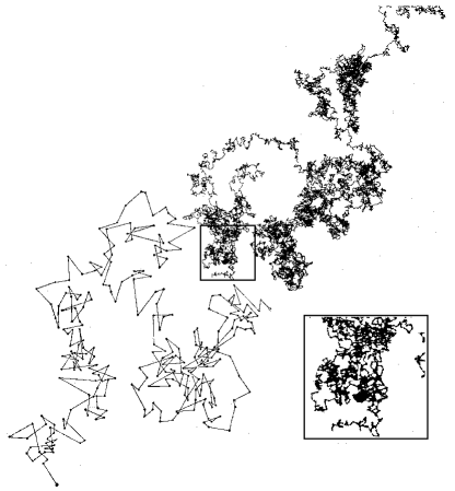
Figure 3: Brownian motion. Bottom left: Strong magnification, showing the discretized aspect of sequential recordings of the position of a particle in suspension, observed by Jean Perrin and his collaborators. Bottom right: Magnification showing the self-similarity of the continuous Brownian curve.

The conclusion was “the rigorous exactness of the formula proposed by Einstein,” and “that some unknown complication or unknown cause of systematic error oddly affected the results of Victor Henri.” They then deduced a new average value of Avogadro’s number, $\mathcal{N}=7.15\times 10^{23}$. A wonderful verification was at last made of “Maxwell’s irregularity law,” that is, of the Gaussian distribution (26) of the Brownian particle’s position in a plane orthogonal to gravity.

Jean Perrin did not stop there, but turned to rotational Brownian motion. Einstein himself did not really think that his predictions (41) were experimentally verifiable, because the speed of rotation seemed to be too large to be observable. In fact, for grains of 1 $\mu$m in diameter, the rotation is about 1 degree per hundredth of second. Perrin could then prepare spheres with larger diameter, from 10-15 $\mu$m up to 50 $\mu$m, and he succeeded in preparing them in suspension in a 27% solution of urea. In this case the angular speed falls to a few degrees per minute. The spheres carried inclusions of different refractive indices, which made their rotation observable under a microscope! The result was a spectacular verification of Einstein’s second formula (41), this time for grains 100 000 times heavier than the small grains of gamboge first studied. On 11 November 1909, Einstein wrote to Perrin: “I would not have considered a measurement of rotations as feasible. In my eyes it was only a pretty triffle”.

Perrin received the Nobel Prize in 1926 for his work on Brownian motion. His book, Atoms, one of the most finely written physics books of the 20th century, contains a postmortem, in the great classic style, about the fight for establishing the reality of molecules:

“La théorie atomique a triomphé. Encore nombreux naguère, ses adversaires enfin conquis renoncent l’un après l’autre aux défiances qui, longtemps, furent légitimes et sans doute utiles. C’est au sujet d’autres idées que se poursuivra désormais le conflit des instincts de prudence et d’audace dont l’équilibre est nécessaire au lent progrès de la science humaine.”

“The atomic theory has triumphed. Its opponents, who until recently were numerous, have been convinced and have abandoned one after the other the sceptical position that was for a long time legitimate and likely useful. Equilibrium between the instincts towards caution and towards boldness is necessary to the slow progress of human science; the conflict between them will henceforth be waged in other realms of thought.”

To conclude this section, let us return for a last time to Einstein. One reads in his autobiographical notes:

“The agreement of these considerations with experience together with Planck’s determination of the true molecular size from the law of radiation (for high temperatures) convinced the sceptics, who were quite numerous at that time (Ostwald, Mach) of the reality of atoms. The antipathy of these scholars towards atomic theory can undubitably be traced back to their positivistic philosophical attitude. This is an interesting example of the fact that even scholars of audacious spirit and fine instinct can be obstructed in the interpretation of facts by philosophical prejudices. The prejudice –which has by no means died out in the meantime– consists in the faith that facts by themselves can and should yield scientific knowledge without free conceptual construction. Such a misconception is possible only because one does not easily become aware of the free choice of such concepts, which, through verification and long usage, appear to be immediateley connected with the empirical material.”

Let us finally mention Ostwald’s magnanimous concession: In 1908 he refers to the Brownian motion results and says they “entitle even the cautious scientist to speak of the experimental proof for the atomistic constitution of space-filled matter”. In 1910, he is the first person to nominate Einstein for the Nobel Prize (for special relativity).

2 Measurements by Brownian fluctuations

Jumping ahead a century, we observe how the theory of Brownian fluctuations, whose construction we just described, today finds spectacular applications in physics applied to biology. We will give an example from the physics of DNA.

2.1 Micromanipulation of DNA molecules

2.1.1 The interest of DNA for physicists

Physicists are interested today in DNA for several reasons. First, it is a remarkable polymer for its length, reaching several centimeters, and for its monodispersity (the DNA of the virus bacteriophage-$\lambda$, for example, always has 48502 base pairs in the identical sequence). DNA is an important subject in polymer physics because it can be easily shaped by bio-molecular tools and it can be directly observed and manipulated. A fluorescent intercalation placed between base pairs (such as ethidium bromide) permits the observation, under a microscope and by fluorescence, of single DNA molecules in solution.

2.1.2 Experimental realization of a micro-manipulation

One can also micro-manipulate molecules individually. The techniques of micro-manipulation of isolated bio-molecules have developed considerably during the past few years, thanks to an ever-growing number of tools: optical or magnetic “tweezers,” atomic force microscopes, glass micro-fibers, and also hydrodynamic flow observations.

A recent example consists in pulling a single DNA molecule to measure its extension as a function of the force, which allows one to measure various important mechanical parameters of the DNA chain.

In “magnetic tweezers” (figure 4), a magnetic bead is placed in the field of a magnet; the bead is attracted towards regions with a high gradient field, and one can move the magnets or rotate them. This allows one to pull the DNA or to twist it, creating as well torsions, or super-coilings, that are a part of topological configurations for biological functions.

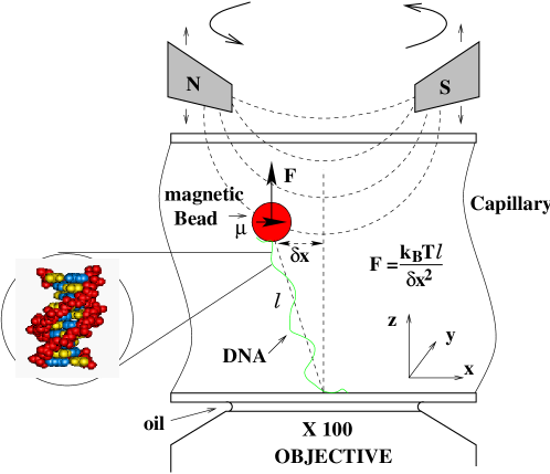
Figure 4: Micro-manipulation of a DNA molecule by “magnetic tweezers”.

We give a brief overview of forces playing a role in biology, and of the specific problems related to their smallness.

2.1.3 Biological interaction forces and thermal agitation forces.

The interaction forces in biological systems are typically generated by hydrogen or ionic bonds, as well as by van der Waals interactions that shape nucleic acids and proteins. Their order of magnitude is typically obtained by dividing $k_{B}T$, the order of magnitude of the “quantum of energy” provided by the hydrolysis of the ATP in ADP (10 $k_{B}T$), by the characteristic size of biological objects, of the order of a nanometer (nm). We then find the picoNewton:

$$\frac{k_{B}T}{1{\rm nm}}=4\underset{\begin{subarray}{c}\|\\ 10^{-12}\text{ N}\end{subarray}}{\text{p}N}.$$

Figure 5: The track of the random displacement, in a liquid, of the tip of the cantilever in an atomic force microscope. It executes a one-dimensional Brownian motion. (Kindly provided by Pascal Silberzan and Olivia du Roure, Curie Institute.)

Such a force is the one typically needed to stretch a DNA molecule. As it is extremely small, it is not easy to detect with standard measuring devices.

The smallest measurable forces are in principle limited by the thermal agitation of the measuring device (see figure 5). This thermal agitation generates Langevin’s stochastic force seen above, whose value depends on the coefficient of viscous friction of the object, and also on the temporal window of observation. We have:

$$\langle X^{2}_{\text{Langevin}}\rangle=2k_{B}T\;6\pi\eta\;a\,\delta f,$$

where $\eta$ is the medium’s viscosity, $a$ the radius of a spherical bead taken as an example, and $\delta f$ the observed frequency range. For example, for $a=1.5\;\mu{\rm m}$, in water (viscosity $\eta\simeq 10^{-2}$ Poise = $10^{-3}$ Pa/s), the average force over a period of a second is $X_{\text{Langevin}}\sim 15\underset{\begin{subarray}{c}\|\\ (10^{-15}\text{ N})\end{subarray}}{f\text{N}}$, i.e., 15 femtoNewtons.

Astonishingly, Brownian fluctuations can be used directly to measure forces of biological origin!

2.2 Measurement of force by Brownian fluctuations

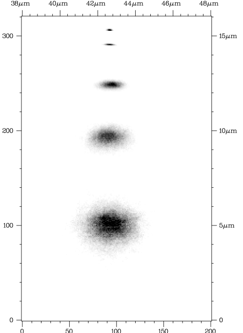
Figure 6: Brownian cloud of a bead’s fluctuating position in the vertical plane $(Ox,Oz)$, for different applied forces. The larger the force, the more a molecule is stretched, and the more the Brownian fluctuations are constrained. (Figure kindly provided by Vincent Croquette, Statistical Physics Laboratory, ENS, Paris.)

This technique of measuring a force is largely inspired by the method proposed by Einstein for measuring the elastic constant of a spring by means of Brownian fluctuations. When we apply a force upon a small magnetic bead in a gradient field, the stretched molecule and the bead form a minuscule pendulum of length $\ell$ (figure 4). The bead is animated by Brownian motion, connected to the thermal agitation of surrounding water molecules. The small magnetic pendulum is thus perturbed from its equilibrium position by Langevin’s random force. It is then brought back towards equilibrium by the pulling force exerted by the DNA (figure 6).

As we will show in detail further along, the pendulum possesses a transverse elastic constant $k_{\perp}$ that is directly related to the pulling force $F$ by $k_{\perp}=F/\ell$. If we call $x$ the position of the bead with respect to its equilibrium position in the direction perpendicular to the force $\vec{F}$, the theory states

$$F=k_{B}T\ell/\langle x^{2}\rangle,$$

where $\langle x^{2}\rangle$ is the average quadratic fluctuation of $x$. To measure the pulling force on a DNA molecule, one simply measures the length $\ell$ and the average quadratic fluctuation $\langle x^{2}\rangle$! This is reminiscent of Einstein’s formula (28), as well as of the surprise of being able to deduce Avogadro’s number from it.

To measure such fluctuations, one must follow the movements of the bead during a given amount of time, just as in Jean Perrin’s experiments of 1908 on Brownian motion. Today, a computer program analyzes in real time the images on a video of the bead observed via a microscope, and determines its positions in a three-dimensional space with a precision of 10 nm (figure 6). Such precision is obtained through a technique of image correlation.

This sort of Brownian measurement has several advantages:
- One gauges the force by absolute measurement of position fluctuations;
- There is no contact with the bead, therefore it is non-invasive;
- The range of values of $x$ is between $\mu$m to nm, the force goes from a dozen femtoNewtons to hundreds of picoNewtons.
The drawback is its slowness: to accumulate sufficient fluctuations and to have reliable statistics, a minute of recording is needed for a force of 1pN, and more than an hour for 10fN.

We shall now describe the theory of measurement by Brownian fluctuations.

2.3 Theory

2.3.1 Equilibrium and fluctuations

Figure 7: Axis of a DNA chain fluctuating around the vertical position; the extremity $M$ moves from the equilibrium position $(0,0,\ell)$ in presence of $F$ towards the random position $(x,y,\ell+z)$.

One considers a DNA chain of length $\ell_{0}$ with one extremity fixed at the origin $0$, while the other extremity $M$ is determined by $\overrightarrow{{OM}}=\vec{r}$ (see figure 7). A force $\vec{F}$ acts on the extremity $M$ along the direction of the $Oz$ axis. At equilibrium, the chain is parallel to the $Oz$ axis and is elastically stretched up to a length $\ell$ dependent on $F$. The Brownian fluctuations, originating from the shocks between the bead that is attached to the DNA chain and the molecules of the solution, induce small displacements $(x,y,z)$ that one can consider as perturbations of the macroscopic equilibrium position (0,0,$\ell$). The extremity $M$ is thus shifted from its equilibrium position $(0,0,\ell)$ (in the presence of $F$) to a random position $(x,y,\ell+z)$. Let $r=|\overrightarrow{{OM}}|$ be the radial distance between the extremities of the chain. Because of elasticity, the chain develops a restoring radial force $F_{r}(r)$. At equilibrium, one has $F_{r}(\ell)=F$, where $F$ is the external force given experimentally.

In the presence of fluctuations, the radial distance is written

$$r=[(\ell+z)^{2}+x^{2}+y^{2}))]^{1/2},$$ (80)

and the restoring force

$$\vec{F}_{r}=-\frac{\vec{r}}{r}F_{r}(r)=\begin{cases}F_{rx}=-\displaystyle\frac{x}{r}F_{r}(r)\\[11.38092pt] F_{ry}=-\displaystyle\frac{y}{r}F_{r}(r)\\[11.38092pt] F_{rz}=-\displaystyle\frac{\ell+z}{r}F_{r}(r).\end{cases}$$ (81)

2.3.2 Series expansions

One writes the series expansion of the distance $r$ for $x,y,z$ small compared to $\ell$:

$$r=[(\ell+z)^{2}+x^{2}+y^{2}]^{1/2}=\ell+z+\cdots$$ (82)

An expansion to the first linear order in $x,y,z$ will be sufficient, and from now on we will denote by $+\cdots$ all second order terms (of $O(x^{2},y^{2},z^{2})$) in the expansions.

The radial force $F_{r}(r)$ of the DNA on the bead, depends only on the radial distance $r$; therefore, from (82), it has the series expansion:

$$F_{r}(r) = F_{r}\left[\ell+z+\cdots\right]=F_{r}(\ell)+z\frac{d\,F_{r}}{d\,r}(\ell)+\cdots.$$ (83)

One can now easily determine the components (81) of the radial force by using (82) and (83):

$$F_{rx} = -\frac{x}{r}F_{r}(r)=-\frac{x}{\ell}F_{r}(\ell)+\cdots,$$

$$F_{ry} = -\frac{y}{r}F_{r}(r)=-\frac{y}{\ell}F_{r}(\ell)+\cdots,$$

$$F_{rz} = -\frac{\ell+z}{r}F_{r}(r)=-F_{r}(\ell)-z\frac{d\,F_{r}}{d\,r}(\ell)+\cdots.$$

We finally note that at the equilibrium point the external force, $\vec{F}=F\vec{u}_{z}$, exactly cancels the term $-F_{r}(\ell)\vec{u}_{z}$ of the vertical component $F_{rz}\vec{u}_{z}$. Leaving aside terms of second order, our analysis leads us to a fluctuating resultant force on the DNA :

$${\vec{f}}=F\vec{u}_{z}+{\vec{F}_{r}}=\begin{cases}-\displaystyle\frac{x}{\ell}F_{r}(\ell)\\[11.38092pt] -\displaystyle\frac{y}{\ell}F_{r}(\ell)\\[11.38092pt] -z\displaystyle\frac{dF_{r}}{d\ell}(\ell)\end{cases}\quad{=-\nabla_{\vec{r}}\,U.}$$ (84)

2.3.3 Elastic energy

The beauty of this approach is that one can determine the elastic energy of the Brownian fluctuations of the DNA chain without even knowing the analytic form of the elastic force. In these expressions, it must be understood that the equilibrium length $\ell$ is determined by the external force, while the fluctuating force (84) is linear in $x,y,z$, as expected from an expansion to first order. A quadratic potential energy $U$ is associated to the force by ${\vec{f}}=-{\nabla}_{\vec{r}}\,U$, given by the simple expression:

$$U=\frac{1}{2}\left({x^{2}}+{y^{2}}\right)\frac{1}{\ell}F_{r}(\ell)+\frac{1}{2}z^{2}\frac{d\,F_{r}}{d\,\ell}(\ell).$$ (85)

2.3.4 Elastic constants

One can write the energy $U$ (85) as that of a three-dimensional anisotropic harmonic oscillator with two elastic constants, $k_{\perp}$ and $k_{\parallel}$, corresponding to the perpendicular and parallel directions, respectively, with respect to the force:

$$U=\frac{1}{2}k_{\perp}\left({x^{2}}+{y^{2}}\right)+\frac{1}{2}k_{\parallel}\,z^{2},$$ (86)

with

$$\begin{cases}k_{\perp}&=\displaystyle\frac{F_{r}(\ell)}{\ell},\\[11.38092pt] k_{\parallel}&=\displaystyle\frac{d\,F_{r}}{d\,\ell}(\ell).\end{cases}$$ (87)

As one can intuitively imagine, the transverse elastic constant, which opposes lateral movements of the DNA molecule, is weaker than the longitudinal elastic constant, which opposes mechanical stretching of the DNA.

2.3.5 Energy equipartition

In classical statistical mechanics, we have seen the historically important result about the equipartition of energy. The theory simply states that each quadratic degree of freedom has average energy $\frac{1}{2}k_{B}T$ exactly, where $k_{B}$ is Boltzmann’s constant and $T$ is the absolute temperature. In the case of the harmonic energy (86), the theorem immediately gives us:

$$\frac{1}{2}k_{\perp}\langle{x^{2}}\rangle=\frac{1}{2}k_{\perp}\langle{y^{2}}\rangle=\frac{1}{2}k_{\parallel}\,\langle z^{2}\rangle=\frac{1}{2}k_{B}T\,.$$ (88)

Therefore we find, with the help of (87)

$$\begin{cases}k_{\perp}&=\displaystyle\frac{F_{r}(\ell)}{\ell}=\frac{k_{B}T}{\langle{x^{2}}\rangle}\,,\\[11.38092pt] k_{\parallel}&=\displaystyle\frac{d\,F_{r}}{d\,\ell}(\ell)=\frac{k_{B}T}{\langle{z^{2}}\rangle}\,.\end{cases}$$ (89)

Because of the difference between the elastic constants, $k_{\perp}<k_{\parallel}$, transverse fluctuations dominate over longitudinal ones: $\langle{x^{2}}\rangle=\langle{y^{2}}\rangle>\langle{z^{2}}\rangle$, as one can see in figure 6. One sees, for instance, that the fluctuations $\sqrt{\langle{x^{2}}\rangle}$ and $\sqrt{\langle{z^{2}}\rangle}$ are of the order of $2\,\mu{\rm m}$ and of less than $1\,\mu{\rm m}$, respectively, for the second Brownian cloud from the bottom. Such Brownian fluctuations can be directly measured optically, as can the length $\ell$, and equation (89) allows a truly ingenious direct measurement of the elastic force $F_{r}(\ell)$ and its derivative ${F_{r}^{{}^{\prime}}(\ell)}$! One can then compare the experimental results to the predictions of theoretical models for the statistical description of the DNA configurations (see figure 8).

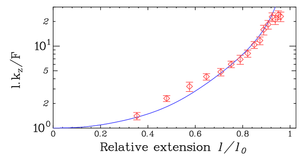
Figure 8: Dimensionless ratio $\frac{\ell k_{z}}{F}=\frac{k_{\parallel}}{k_{\perp}}=\frac{\langle{x^{2}}\rangle}{\langle{z^{2}}\rangle}=\frac{\ell}{F_{r}(\ell)}\frac{d\,F_{r}}{d\,\ell}(\ell),$ plotted as a function of the length $\ell$ of the DNA chain (in units of maximum length $\ell_{0}$). The points correspond to the ratio of experimental measurements of transverse ($\langle{x^{2}}\rangle$) and vertical ($\langle{z^{2}}\rangle$) quadratic Brownian fluctuations. The curve is theoretically predicted from the knowledge of $F_{r}(\ell)$, in a model of a semi-flexible DNA chain, also known as the Worm-like Chain Model. We stress the remarkable agreement between experiment and theory. (Figure kindly provided by Vincent Croquette.)

3 Potential theory and Brownian motion

Et ignem regunt numeri

3.1 Introduction

3.1.1 Laplace’s equation

Potential theory concerns the equilibrium properties of continuous bodies, like the distribution of electrostatic charges on conductors, the distribution of the Newtonian potential in the classic theory of gravitation, the distribution of temperature in Fourier’s theory of heat conduction, or in addition the distribution of positions of a stretched elastic membrane.

A deep relation exists between potential theory and the theory of diffusion, and therefore also with Brownian motion. We will first give an intuitive illustration within the framework of Fourier’s theory of heat conduction.

The temperature of a body, $u(x,y,z;t)$ at the point ${x,y,z}$ and at the instant $t$, follows the equation of heat

$$\frac{\partial u}{\partial t}=D\Delta u,$$ (90)

where, as in the case of Brownian motion, $D$ is the diffusion coefficient, and $\Delta$ is the Laplacian in three-dimensions $\Delta=\frac{\partial^{2}}{\partial x^{2}}+\frac{\partial^{2}}{\partial y^{2}}+\frac{\partial^{2}}{\partial z^{2}}$. In general, the Laplacian in $d$ dimensions is:

$$\Delta=\sum_{i=1}^{d}\frac{\partial^{2}}{\partial x_{i}^{2}},$$ (91)

where $x_{i}$ are $d$-dimensional Cartesian coordinates. When the temperature reaches equilibrium, the time dependence cancels, and the temperature field is described by Laplace’s equation:

$$\Delta u=0.$$ (92)

Any function with zero Laplacian is called harmonic.

Such a function, the potential, therefore can be seen as the equilibrium solution of a diffusion process (at infinite time), which is the first elementary relation we meet between potential theory and Brownian diffusion. To specify in our example the value of the temperature everywhere, we must fix the initial conditions in case one starts from an out-of-equilibrium situation.

In the case we will consider here, we want to directly study equilibrium and the associated harmonic functions, or more generally the potential. For that purpose one must know either the position of the sources of the potential, or the boundary conditions on it, in a way that will be made more precise in the following.

Giving the position of the sources is natural in the well-known theory of the Newtonian or Coulomb potential, where the sources of the potential are masses or electrostatic charges. Imposing boundary conditions on the potential is also possible, as is natural in the case of heat conduction and temperature distribution, where one gives the temperature distribution on the surface of a body to determine the internal temperature distribution.

Such representations are mathematically equivalent. Let us first recall the elementary properties of the Newtonian or Coulomb potential that will be useful for obtaining the finer properties of harmonic functions. To fix the ideas, we will adopt the familiar language of a Newton or Coulomb potential created by masses or electrostatic charges, but the mathematical results of course will not depend on this choice.

3.2 Newtonian potential

3.2.1 The potential created by a point source

In order to consider the potential in a universal way, as for gravitation or electrostatics, the physical constants like the universal gravitational constant $G$, or the electric permeability of the vacuum, $\varepsilon_{0}$, are not indicated. In general, we will adopt the electrostatic language.

The potential at a point $P$ in three dimensions created by a unit charge or mass placed at the origin $O$ is

$$u_{3}(r)=\frac{1}{4\pi r},\;\;r=|\overrightarrow{OP}|,$$ (93)

where $r$ is the distance between $O$ and $P$ (figure 9).

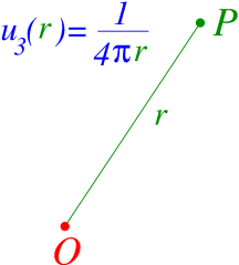
Figure 9: Newtonian potential in three dimensions.

The associated electric (or gravitational) field is

$$\vec{E}_{3}(\vec{r})=-\nabla_{\vec{r}}\,u_{3}(r)=\frac{1}{4\pi}\frac{\vec{r}}{r^{3}},$$ (94)

where $\vec{r}$ is the relative position vector $\vec{r}=\overrightarrow{OP}$.

In $d$ dimensions, the potential and field generalize to

$$u_{d}(r)=\frac{1}{(d-2)S_{d}}\frac{1}{r^{d-2}},$$ (95)

and

$$\vec{E}_{d}(\vec{r})=-\nabla_{\vec{r}}\,u_{d}(r)=\frac{1}{S_{d}}\frac{\vec{r}}{r^{d}},$$ (96)

where $S_{d}=2\pi^{d/2}/\Gamma(d/2)$ is the surface of the unit sphere in $\mathbb{R}^{d}$.

The two-dimensional case is more complicated, and leads to a logarithmic potential,

$$u_{2}(r)=\frac{1}{2\pi}\log\frac{1}{r},$$ (97)

$$\vec{E}_{2}(\vec{r})=-\nabla_{\vec{r}}\,u_{2}(r)=\frac{1}{2\pi}\frac{\vec{r}}{r^{2}}.$$ (98)

3.2.2 Laplace’s equation and the Dirac distribution

The Laplacian of the above potential $u_{d}(r)$ vanishes identically everywhere in space, except at the origin: $\Delta u_{d}(r)=0,\;r\neq 0$. At $\vec{r}=\vec{0}$ it is divergent, and its value is given by a distribution, namely

$$\Delta u_{d}(r)=\frac{1}{(d-2)S_{d}}\Delta\frac{1}{r^{d-2}}=-\delta^{d}(\vec{r}),$$ (99)

where $\delta^{d}(\vec{r})$ is the Dirac distribution in $d$ dimensions, zero everywhere except at the origin $\vec{r}=\vec{0}$, where it is singular (infinite). This divergence is such that the integral

$$\int_{\mathbb{R}^{d}}f(\vec{r})\delta^{d}(\vec{r})\,{\rm d}^{d}r=f(\vec{0})$$ (100)

yields the value at the origin of any test function $f(\vec{r})$.

Equation (99) is Poisson’s equation, where the second term represents the mass or charge density, i.e., the source of the potential. In the case of a potential (93), (95) or (97), such a source is a point, at which a singular density appears.

In the elementary approach that follows, we shall not use this formalism. Rather, we will follow the elementary path that uses Gauss’ theorem.

3.2.3 Gauss’ theorem

Gauss’ theorem says that the flux of an electric (or gravitational) field across any closed surface $\Sigma$ is equal to the total charge $Q(\Sigma)$ (or mass) enclosed by the surface:

$$\int_{\Sigma}\vec{E}\cdot\,{d\vec{S}}=Q(\Sigma).$$ (101)

This theorem can be proved in two stages. By linearity, since the case of a distribution of charges can be treated by adding the fields, one can reduce it to the case of a point charge. Actually, if each one of these fields satisfies Gauss’ theorem, their sum will as well.

Next, for a point charge enclosed by the surface, we notice that the flux of $\vec{E}$ is invariant when we deform the surface $\Sigma$ without crossing the charge. We can thus restrict attention to a sphere around the charge, for which Gauss’ theorem is trivial. Actually, because of the form (94) of the $1/r^{2}$ field with spherical symmetry, the integral (101) on a sphere of a radius $r$ is equal to the charge.

Gauss’ theorem immediately generalizes to any number of dimensions.

3.2.4 Potential generated by a sphere

Let us consider the sphere $\mathcal{S}(a)$ of radius $a$ centered at the origin $O$. Imagine that it carries a charge $Q$ uniformly distributed over its surface.

The associated field $\vec{E}(r)$ is radial and with spherical symmetry. It satisfies Gauss’ theorem (101). If we choose the surface $\Sigma$ as a sphere $\mathcal{S}(r)$ centered at $O$, of radius $r>a$, i.e., exterior to $\mathcal{S}(a)$, we have $Q(\Sigma)=Q$, and the flux of $\vec{E}(r)$ across $\Sigma$ is simply, by spherical symmetry, $E(r)4\pi r^{2}=Q$. We then deduce that $E(r)=\frac{Q}{4\pi r^{2}}$ is the same field that would be created by a charge as if it was concentrated at the center of sphere. If the surface $\Sigma$ is chosen like a sphere $\mathcal{S}(r)$ of radius $r<a$, i.e., inside $\mathcal{S}(a)$, then $Q(\Sigma)=0$ and the flux (101) is then zero. By symmetry, we then deduce that the field $\vec{E}$ is zero everywhere inside the sphere.

Let $u_{\mathcal{S}}(P)$ now be the potential created at a point $P$ by the same sphere $\mathcal{S}(a)$ of radius $a$ with total charge $Q$, uniformly distributed on the surface. This potential has a spherical symmetry, as does its associated field. Outside the sphere, the field is the same as that of a point charge $Q$ placed at the center, while inside the sphere the field is zero. The potential outside the sphere is therefore the one, (93), created by a point charge placed at the center of the sphere, while inside the sphere it is constant, and by continuity equal to its value on the boundary. One thus has

$$u_{\mathcal{S}}(P)=\frac{1}{4\pi}\frac{1}{r}\vartheta(r-a)+\frac{1}{4\pi}\frac{1}{a}\vartheta(a-r),\;\;r=|\overrightarrow{OP}|,$$ (102)

where $\vartheta$ is the Heaviside distribution $\vartheta(x<0)=0,\;\vartheta(0)=1/2,\;\vartheta(x>0)=1$.

3.3 Harmonic functions and the Theorem of the Mean

3.3.1 Gauss’ theorem of the Arithmetic Mean

The property that two bodies or two charges attract one another with equal and opposite forces, reflects itself in the potential. Actually the potential is symmetric with respect to the coordinates of the two points, in such a way that the potential at $P$ of a charge $Q$ at $S$ is the same as the potential at $S$ of a charge $Q$ at $P$. From such a simple fact follow theorems with important applications. We derive two of them, called Gauss’ theorems of the Arithmetic Mean.

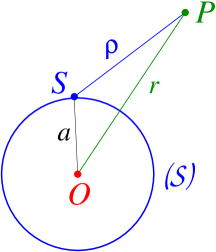
Figure 10: Newtonian potential (103) created by a uniformly charged sphere of radius $a$.

The potential

$$u_{\mathcal{S}}(P) = \frac{Q}{4\pi a^{2}}\int_{\mathcal{S}}\frac{d^{2}S}{4\pi\rho},\;\rho=|\overrightarrow{SP}|$$ (103)

is the one at point $P$, created by all points $S$ on the surface of a sphere $\mathcal{S}$ of radius $a$, and with uniform charge density $\frac{Q}{4\pi a^{2}}$ (see figure 10). In (102) we just saw that outside the sphere the potential is equal to $\frac{Q}{4\pi r}$, where $r$ is the distance $r=|\overrightarrow{OP}|$, while inside the sphere it is constant and equal to $\frac{Q}{4\pi a}$.

But because of the exchange symmetry which we just mentioned, the potential can also be interpreted as the arithmetic mean on the surface of a sphere of the potential created by the same charge $Q$, this time placed in $P$.

The equations (102) (103) therefore have the following interpretation:
a) The average on the surface of a sphere of the potential created by a charge situated outside the sphere, and at a distance $r$ from its center, is equal to the value (varying as ${1}/{r}$) of the potential at the center of the sphere;
b) The average on the surface of a sphere of the potential created by a charge in any position inside the sphere, is equal to the value (varying as ${1}/{a}$) of the potential on the sphere, after concentrating the whole charge at the center of the sphere.

Now let us suppose that we have a group of charges placed either entirely on the outside of the sphere, or entirely on the inside. By adding up the above results for each elementary charge, we find the following two generalizations:
a) Gauss’ Theorem of the Arithmetic Mean: the average on a surface of a sphere of the potential created by charges situated entirely outside the sphere is equal to the value of the potential at the center;
b) The Second Theorem of the Mean: the average of the potential on a surface of a sphere, created by charges situated entirely inside the sphere, is independent of their distribution inside the sphere, and it is equal to the total charge divided by the radius of the sphere.

3.3.2 Harmonic functions

Finally let us come back to harmonic functions, and consider a function $u$ such that $\Delta u=0$ in some domain $\mathcal{D}$. Such a harmonic function can be represented as a potential created inside the domain $\mathcal{D}$ by a distribution of charges outside $\mathcal{D}$. We can then apply the first of Gauss’ theorems, and obtain the mean-value theorem for harmonic functions: The average of a harmonic function $u$ on a sphere $\mathcal{S}$ centered at a point P is equal to the value of $u$ at $P$. For instance, in three dimensions:

$$u(P)=\int_{\mathcal{S}}u(S)\frac{d^{2}S}{4\pi a^{2}},$$ (104)

where $a$ is the radius of the sphere; the theorem can be generalized to any number of dimensions.

The reciprocal is also true: any function that fulfills the Theorem of the Mean on every sphere inside a given domain, is harmonic inside that domain. This theorem is going to be the key relation between potential theory and Brownian motion.

3.4 The Dirichlet problem

A classic problem of potential theory is that of Dirichlet. One considers a domain $\mathcal{D}$ of the Euclidean space $\mathbb{R}^{d}$ and its boundary $\partial\mathcal{D}$. The potential $u$ is given on the boundary by means of a given continuous function $f$:

$$\Delta u = 0\;\;{\rm inside}\;\;\mathcal{D},$$ (110)

$$u = f\;\;{\rm on}\;\;\partial\mathcal{D}.$$ (111)

For instance, the Dirichlet problem in the case of heat conduction is to determine the equilibrium temperature inside a conducting body $\mathcal{D}$, once the distribution $f$ of the temperature along the boundary $\partial\mathcal{D}$ is given.

It is here that Brownian motion comes into play, to provide an entirely probabilistic representation of the solution.

3.5 Relation between potential theory and Brownian motion

3.5.1 Newtonian potential and probability density

The first relation, which contains the kernel of all the others, is obtained simply by considering the Gaussian probability density (26), which represents the probability density of finding a Brownian particle at a point $\vec{r}$ at time $t$, knowing that the particle was at the origin at time $t=0$. In $d$ dimensions, formula (26) generalizes to

$$P(\vec{r};t)=\frac{1}{(4\pi Dt)^{d/2}}\exp{\left(-\frac{r^{2}}{4Dt}\right)},$$ (112)

where $r$ is the distance from the origin.

By integrating $P(\vec{r};t)$ over the time variable $t$ one obtains

$$D\int_{0}^{+\infty}P(\vec{r};t)\,{\rm d}t=\frac{1}{(d-2)S_{d}}\frac{1}{r^{d-2}}=u_{d}(r).$$ (113)

For a unit diffusion coefficient $D=1$, the total Brownian probability density of arriving at $\vec{r}$ at any time is then exactly equal to the Newtonian potential created at $\vec{r}$ by a unit charge or mass.

Let us look now at the Dirichlet problem from a more general point of view.

3.5.2 Discrete random walks and the Dirichlet problem

This problem was considered in the 1920’s with the work of Phillips and Wiener, and of Courant, Friedrichs and Lewy. They obtained a probabilistic representation of the solution of the Dirichlet problem (110, 111), in the form of an approximate sequence of random walks on a $d$-dimensional cubic lattice $\varepsilon\mathbb{Z}^{d}$, of lattice spacing $\varepsilon$.

More precisely, one considers random walkers $w=\{w_{n},n\in\mathbb{N}\}$ on the lattice $\varepsilon\mathbb{Z}^{d}$, at discrete times $n=0,1,2,\cdots$, all starting from the initial point $w_{0}=P$ in domain $\mathcal{D}$ and diffusing away. When the walkers ultimately reach the boundary, one measures the value of the function $f$ at that point on the boundary. One repeats the process and then takes the average of the values of the function $f$ over all first contact points on the boundary reached by random walkers that started from $P$.

We can formally write the averaging operation as

$$u_{\varepsilon}(P)=\sum_{{\{w:\;w_{0}=P\}}}\frac{1}{(2d)^{\tau_{\mathcal{D}}}}f(w_{\tau_{\mathcal{D}}}),$$ (114)

where the sum is over all random walks $w=\{w_{n},n\in\mathbb{N}\}$ on the lattice $\varepsilon\mathbb{Z}^{d}$, at discrete times $n=0,1,2,\cdots$, leaving the initial point $w_{0}=P$ and diffusing towards the boundary. In (114), $\tau_{\mathcal{D}}$ is the first instant at which the boundary $\partial\mathcal{D}$ is reached by the random walker, and $w_{\tau_{\mathcal{D}}}$ its position on the boundary at this instant. The sum must be normalized by the inverse of the total number $(2d)^{\tau_{\mathcal{D}}}$ of walks of length $\tau_{\mathcal{D}}$, in a way to be a probability measure on the set of discrete random walkers.

To extend the result in the continuum, one next takes the limit of the lattice spacing $\varepsilon$ to $0$. The result $\lim_{\varepsilon\to 0}u_{\varepsilon}(P)=u(P)$ is then the value of $u$ at point $P$, which is the solution of the Dirichlet problem in $\mathbb{R}^{d}$.

In the language of heat theory for instance, the temperature at point $P$ is the average of the temperature at the boundary, evaluated after random walking towards it! In mathematics, a standard notation of the average (114) is

$$u_{\varepsilon}(P)=\int f(w_{\tau_{\mathcal{D}}})\Pi_{P}^{\varepsilon}{(dw)},$$ (115)

where $\Pi_{P}^{\varepsilon}$ is the probability measure on discrete random walks in $\varepsilon\mathbb{Z}^{d}$ started at $P$.

3.5.3 Norbert Wiener

A first attempt to define integral calculus over a function space was made by Daniell (circa 1920). A few years later, Norbert Wiener introduced a measure in function space which is rigorous from a mathematical point of view (it is a bona fide Borel measure), and which made it possible to define and calculate an integral over a space of functions.

Wiener had indeed known Einstein’s theory since his visit to Cambridge in 1913. At 19, he came to study logic with Bertrand Russell, who suggested that he go listen to Hardy, the mathematician, and read Einstein!

So, motivated also by his reading of Perrin, Wiener constructed, in his fundamental article of 1923, “Differential Space,” a probability measure for Brownian paths in $\mathbb{R}$ (then in $\mathbb{R}^{d}$). The basic idea was to directly construct on the space of continuous functions $w(t)$ of a single real variable (representing the position as a function of time), a probability measure such that the changes of the positions $w(t_{i})=x_{i}$, $i=0,\cdots,n$, over disjoint time intervals, $[t_{i-1},t_{i}]$, $i=1,\cdots,n$, have a joint Gaussian probability distribution,

$$P(\{x_{i}\};\{t_{i}\})=\prod_{i=1}^{n}\frac{1}{[4\pi D(t_{i}-t_{i-1})]^{1/2}}\exp{\left[-\frac{(x_{i}-x_{i-1})^{2}}{4D(t_{i}-t_{i-1})}\right]}.$$ (116)

This is a direct generalization of the Brownian displacement distribution (25).

Wiener obtained his measure by using an explicit mapping of the space ${\mathcal{C}}$ of continuous functions into the interval (0,1) (minus a set of Lebesgue measure zero). This mapping allows to pull-back the ordinary Lebesgue measure on the space ${\mathcal{C}}$. In this language, the Brownian motion has the following probabilistic interpretation: a Brownian path corresponds to the random choice of an element of the measured set ${\mathcal{C}}$ (i.e., a continuous function), endowed with the “Wiener measure”.

Nowadays, this measure is indeed universally called Wiener measure in mathematical circles, while physicists prefer to speak of functional integrals, even though, like Monsieur Jourdain, they really calculate with the Wiener measure when they perform their formal calculations!

The integral over such a measure is called the Wiener average. It is denoted ${\mathcal{W}}({dw})$ here and more precisely ${\mathcal{W}}_{P}({dw})$ for a Brownian motion $w$ started at $P$. It corresponds to the continuous limit for $\varepsilon\to 0$ of the measure $\Pi^{\varepsilon}(dw)$ on random walks on the discrete lattice $\varepsilon\mathbb{Z}^{d}$, introduced in the preceding section.

Once that construction was made, Wiener verified that the measure of the subset of differentiable functions vanishes, in agreement with Perrin’s intuition, and that the support of the measure is given by Hölder functions (of order at least $1/2-\epsilon,\epsilon>0$). In subsequent years, he further developed the very broad ramifications of his theory.

In a study written in 1964 on Wiener and functional integration, Mark Kac highlighted the profound originality of Wiener during his time, and in counterpoint, the difficulty for mathematicians to understand his approach:

“Only Paul Lévy, in France, who had himself been thinking along similar lines, fully appreciated their significance.”

The next steps were indeed made by Paul Lévy, in his great work on Brownian motion, Processus stochastiques et mouvement brownien (1948). Since then, the blooming of the subject in mathematics was such that one can only make an extremely limited citation list. We refer the interested reader to the introductory article of J.-F. Le Gall for a first journey into the Brownian world of mathematics, and to D. Revuz and M. Yor’s book for a more thorough visit.

The connection between the Wiener path measure for Brownian motion and path integrals is perhaps best intuitively understood by considering the multiple distribution (116) for a set of successive equal time intervals, $t_{i}=\frac{i}{n}t,i\in\{1,n\}$. One conditions the path, normalized to start at the origin $x=0$ at time $t=0$, to be at times $t_{i}=\frac{i}{n}t,i\in\{1,n\}$ within intervals ${\rm d}x_{i}$ of the set of points $x_{i}$ in $\mathbb{R}$, and one then takes the formal limit $n\to\infty$:

$${\mathcal{W}}({dw}) = \lim_{n\to\infty}\prod_{i=1}^{n}{\rm d}x_{i}P(\{x_{i}\};\{t_{i}\}))$$ (117)

$$= \lim_{n\to\infty}\prod_{i=1}^{n}{\rm d}x_{i}\prod_{i=1}^{n}\frac{1}{(4\pi D\,{t}/{n})^{1/2}}\exp{\left[-\frac{(x_{i}-x_{i-1})^{2}}{4D\,{t}/{n}}\right]}$$

$$= {\mathcal{D}}w\exp\left(-\frac{1}{4D}\int_{0}^{t}\left(\frac{{\rm d}w(t^{\prime})}{{\rm d}t^{\prime}}\right)^{2}{\rm d}t^{\prime}\right),$$

now with a continuum “Lebesgue” measure on paths,

$${\mathcal{D}}w=\lim_{n\to\infty}\prod_{i=1}^{n}\frac{{\rm d}x_{i}}{(4\pi D\,{t}/{n})^{1/2}}.$$

This notation is marvellously appealing to physicists, since one recognizes in the exponential in (117) the Boltzmann-Gibbs weight associated with the classical kinetic energy of the particle. As Marc Kac noted,

“The disadvantages of such an approach from the purely mathematical point of view are obvious, although it is appealing on formal grounds”.

In $d$ dimensions, the formal equivalence between Wiener’s measure and functional integrals is simply obtained by using the $d$-dimensional Gauss distribution, so that

$${\mathcal{W}}({dw}) = {\mathcal{D}}{w}\exp\left(-\frac{1}{4D}\int_{0}^{t}\left(\frac{{\rm d}{\vec{w}}(t^{\prime})}{{\rm d}t^{\prime}}\right)^{2}{\rm d}t^{\prime}\right),$$ (118)

$${\mathcal{D}}{w} = \lim_{n\to\infty}\prod_{i=1}^{n}\frac{{\rm d}^{d}x_{i}}{(4\pi D\,{t}/{n})^{d/2}}.$$

The rigorous connection between the Wiener path integral and Brownian motion is further illuminated by the Feyman-Kac formula that allows one to write explicit path integral representations for the solutions of parabolic differential equations, corresponding to Brownian motion in presence of a general potential, the case pioneered by Smoluchowski.

When formally continued to imaginary time, the Feyman-Kac formula provides an expression for the Green function of the Schrödinger equation, thus leading to the celebrated path integral representation of Quantum Mechanics invented by Feynman in 1948.

3.5.4 S. Kakutani

The existence of the Wiener measure and Wiener integral allowed for some very important progress by S. Kakutani in 1944-1945. He showed that by substituting an integral with the Wiener measure ${\mathcal{W}}$ in the formula (115) with the discrete measure $\Pi^{\varepsilon}$ indeed solved the Dirichlet problem in continuous space $\mathbb{R}^{d}$. Thus we have Kakutani’s formula

$$u(P)=\int f(w_{\tau_{\mathcal{D}}}){\mathcal{W}}_{P}{(dw)}.$$ (119)

That means that the potential at any point $P$ is given by the average of the potential chosen at random on the boundary by a Brownian motion started at $P$ (figure 11).

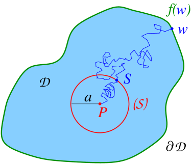
Figure 11: The Dirichlet problem in a domain $\mathcal{D}$, and its Brownian representation. The point $w=w_{\tau_{\mathcal{D}}}$ is the point of first contact of a Brownian motion that started at $P$ with the boundary $\partial\mathcal{D}$, at the instant ${\tau_{\mathcal{D}}}$ of first exit from the domain $\mathcal{D}$. The point $S$ is the point of first passage across the surface of the sphere $\mathcal{S}$.

In the following section we give an elementary demonstration of this result.

3.5.5 Demonstration

In probability theory, the quantity $u(P)$ defined by equation (119) is called the expectation value associated to the point $P$, because it represents the expectation for a random sampling of the value $f$ on the boundary, by a process of Brownian diffusion from $P$.

We want to verify that this expectation value fulfills the two conditions (110) and (111).

The second condition is easy to verify: if the point $P$ is on the boundary $\partial\mathcal{D}$, any Brownian motion $w$ coming from $P$ is immediately stopped on the boundary at $w_{\tau_{\mathcal{D}}}=P$, therefore $u(P)=f(P)$ for $P$ on $\partial\mathcal{D}$, as expected.

Moreover, if the Brownian motion leaves from an internal point $P$, close to a point $P_{0}$ of the boundary, it is (almost) certain (in a probabilistic sense) that the motion will meet the boundary in a neighborhood of $P_{0}$, and that the expectation value $u(P)$ will be close to the value $f(P_{0})$ of $f$ in $P_{0}$. Kakutani’s solution has the right properties of regularity near the boundary, under the condition that the latter has a sufficiently regular geometry and that the “temperature” $f$ on the boundary is a continuous function.

The continuity of the expectation value $u$, with respect to point $P$, is equally clear: a small displacement of $P$ will only slightly modify the Brownian trajectories diffusing from $P$, as well as their subsequent exploration of the boundary.

We will now establish the first property, (110), i.e., that the expectation value $u(P)$ (119) is a harmonic function, by showing that it satisfies the equivalent property (104) on all spheres centered in $P$.

We draw a sphere $\mathcal{S}$ of radius $a$ centered at $P$ and contained inside the domain $\mathcal{D}$ (figure 11). The aim is to show that the Brownian expectation value $u(P)$ obtained by leaving from any point $P$ is equal to the average of Brownian expectation values $u(S)$ obtained from any point $S$ on the surface of the sphere $\mathcal{S}$.

In order to move beyond the boundary $\partial\mathcal{D}$ of the domain, a Brownian motion must cross the sphere $\mathcal{S}$ at least once. Calling $S$ the first crossing point of the sphere (figure 11), and $u(P/S)$ the expectation value obtained for all Brownian motions coming from $P$ and first crossing $\mathcal{S}$ at the point $S$.

As there is no preferential direction for Brownian motion, each point of $\mathcal{S}$ can be met first with equal probability. One distinguishes the average for Brownian motions starting at $P$ in two steps: the choice of the point of first passage $S$, and diffusion across $S$, with the expectation value $u(P/S)$. By averaging the averages, one has the result that $u(P)$ must be equal to the average of $u(P/S)$ on the sphere, i.e., in mathematical terms:

$$u(P)=\int_{\mathcal{S}}u(P/S)\frac{d^{2}S}{4\pi a^{2}}.$$ (120)

The last thing to show is that the expectation value $u(P/S)$, obtained by leaving from $P$ and passing through $S$, is the same as the expectation value $u(S)$, obtained by simply starting from $S$ on the sphere. It is here that a very important property of Brownian motion comes into play: the motion at an instant $t$ only depends on the position at that instant and not on previous motions. Somehow, there is an absolute loss of memory, where only the present instant and position are important: Brownian motion is Markovian. In probability theory, one speaks generally as well of a Markov process when the future dynamic of a process is not influenced by its previous states. The future behavior of a Brownian particle leaving from $S$, or passing through $S$ knowing that it began at $P$, does not differ. It follows that $u(P/S)=u(S)$, which ends the proof of the Theorem of the Mean (104).

3.6 Recurrence properties of Brownian motion

We give an illustration of a non-trivial probabilistic property of Brownian motion, which is deduced from potential theory, that is its recurrence properties.

3.6.1 Brownian motion in one dimension

Let us consider now the one-dimensional real line $\mathbb{R}$ and points $x$ of a domain $\mathcal{D}$, here the line segment $\mathcal{D}=[0,R]$, where $R$ is a positive number. Let us search for the harmonic function $u(x)$ that satisfies the simple Dirichlet problem: $u(0)=0,\;u(R)=1$. In one dimension, the Laplacian (91) is simply the second derivative, so the harmonic equation (110) becomes ${\rm d}^{2}u(x)/{\rm d}x^{2}=0$. The solution is simply linear in $x$: $u(x)=x/R$; it evidently satisfies the required conditions at the boundaries.

Let us consider Kakutani’s solution for the Dirichlet problem by Brownian mathematical expectation. The boundary $\partial\mathcal{D}$ of the segment $\mathcal{D}=[0,R]$ is made up of two points: $\partial\mathcal{D}=\{0,R\}$. The function $f$ with Dirichlet conditions (111), takes the values on the boundary: $f(0)=0,\;f(R)=1$. According to Kakutani’s result, the value $u(x)=x/R$ of the harmonic function $u$ is the average of the function $f$ obtained from random sampling by means of a Brownian motion starting at $x$. The case of the first Brownian exit from the segment $\mathcal{D}=[0,R]$ at point $x=0$ gives a value $f=0$, and at point $x=R$ the value $f=1$. The Brownian expectation of $f$ is thus exactly the probability for the Brownian motion to first exit from the segment $[0,R]$ at the endpoint $R$ rather than at $0$, or else the probability, starting from $x$, to attain $R$ before $0$. The complementary probability to attain $0$ before $R$ is thus $p_{R}(x)=1-u(x)=1-x/R.$

Let us now keep the point $x$ fixed while taking the limit $R\to\infty$, so that the segment $\mathcal{D}$ extends to the positive real axis $\mathbb{R}^{+}$. We see that $p_{R\to\infty}(x)\to 1$, and this is for all $x$. The probability $p_{\infty}(x)$, for a Brownian motion started at $x$, to reach the origin $0$ before leaving to infinity is therefore identically equal to one.

The Brownian motion, wherever it leaves from, passes by the origin (quasi-) certainly. Since spatial and temporal origins were arbitrary in our demonstration, the following property was established: a Brownian motion in one dimension passes through all points on the real axis, infinitely many times. One says it is recurrent in one dimension.

This property did not appear as evident a priori from the probability theory side. Thanks to the relation to potential theory, it has been obtained by simply solving a second order differential equation! Einstein would surely not have thought of this in 1905, although who knows?

Now we will generalize the above study to two and then to $d$ dimensions.

3.6.2 The two-dimensional case

This time, we consider the planar annular domain $\mathcal{D}$, which is that between two concentric circles $\mathcal{C}_{1}$ and $\mathcal{C}_{2}$ centered at the origin $O$, of respective radii $\rho_{1}$ and $\rho_{2}$, with $\rho_{1}<\rho_{2}$. The boundary of the domain $\mathcal{D}$ is then made of two circles, $\partial\mathcal{D}=\mathcal{C}_{1}\cup\mathcal{C}_{2}$. We pose the Dirichlet problem in the annular domain $\mathcal{D}$:

$$\Delta u = 0\;\;{\rm inside}\;\;\mathcal{D},$$ (121)

$$u = 0\;\;{\rm on}\;\;\mathcal{C}_{1},\;\;u=1\;\;{\rm on}\;\;\mathcal{C}_{2}.$$ (122)

By using the two-dimensional Newtonian potential $u_{2}(r)$ (97), it is easy to see that the solution to the Dirichlet problem is spherically symmetric and at a distance $r$ from the center evaluates to:

$$u_{2}(r;\rho_{1},\rho_{2}) = \frac{u_{2}(r)-u_{2}(\rho_{1})}{u_{2}(\rho_{2})-u_{2}(\rho_{1})}=\frac{\log{r}-\log{\rho_{1}}}{\log{\rho_{2}}-\log{\rho_{1}}},\;\;\rho_{1}\leq r\leq\rho_{2}.$$ (123)

Actually, this function obviously satisfies (122) and is harmonic in the annular domain $\mathcal{D}$, because the potential $u_{2}(r)$ (97) is harmonic too (except at the origin, which indeed does not belong to $\mathcal{D}$).

Let us come now to Kakutani’s representation of the solution to the Dirichlet problem. In a manner similar to the one-dimensional case in the preceding paragraph, $u_{2}(r;\rho_{1},\rho_{2})$ (123) represents the probability that a Brownian motion, started at a distance $r$ from the center, hits the outer circle $\mathcal{C}_{2}$ before hitting the inner circle $\mathcal{C}_{1}$.

As in the preceding paragraph, let us fix the distance $r$ and the internal circle $\mathcal{C}_{1}$, and push the boundary of the outer circle $\mathcal{C}_{2}$ to infinity. By taking $\rho_{2}\to\infty$ in formula (123), we see that by continuity the probability that the Brownian motion goes to infinity is $u_{2}(r;\rho_{1},\infty)=0$, for all $r$ and $\rho_{1}$ finite. It means that the Brownian motion reaches the disk of radius $\rho_{1}$ with probability $1$, whatever its point of departure outside of the disk. Since the initial departure time is arbitrary too, likewise the origin in the plane, one then concludes that a two-dimensional Brownian motion passes through neighboring points of any point infinitely often. It is then recurrent in two dimensions, just as it is in one dimension.

It is equally interesting to fix $r$ and $\rho_{2}$ in (123), and to take the limit of an infinitesimal circle around the origin, i.e., $\rho_{1}\to 0$. We then find that by continuity $u_{2}(r;\rho_{1}=0,\rho_{2})=1$. The probability that a Brownian motion starting at a distance $r\neq 0$ from the origin, moves away from the origin up to a distance $\rho_{2}>r$ without having visited the origin at $\rho_{1}=0$, is then equal to $1$. In other words, a Brownian motion that does not leave from the origin $O$ avoids the origin with probability $1$, without ever being able to pass through it.

We deduce an apparently paradoxical result: in two dimensions, any Brownian motion passes through a given point with zero probability, but it passes through immediate neighboring points infinitely often with probability $1$!

Such a double result is due to the presence in the expectation (123) of one function, the logarithm, that diverges both at short distance for $\rho_{1}\to 0$, and at long distance for $\rho_{2}\to\infty$. This is peculiar to two dimensions and announces exceptional properties known as conformal invariance in two dimensions, which will be described in the following section.

In $d>2$ dimensions, a simple power law controls the Newtonian potential $u_{d}(r)$ (95), and only a divergence at short distance appears. We will see the consequences of such a divergence on the recurrence properties of Brownian motion.

Let us mention however that these properties only constitute the “tip of the iceberg”: the singular character of the potential at short distances is the source of divergences in quantum field theories, which led to the creation of renormalization theory, whose consequences have been quite fruitful in the physics of elementary particles and in statistical mechanics. Actually, the intersection of Brownian motions provides the random geometric mechanism that underlies any interacting field theory. This equivalence is fundamental in the theory of polymers and also in the rigorous theory of second order phase transitions. But “Revenons à nos moutons.”

3.6.3 The $d$-dimensional case

We are now well enough equipped to pass to the $d$-dimensional case, for $d>2$. Let us consider two concentric hyperspheres, $\mathcal{S}_{1}$ and $\mathcal{S}_{2}$, centered at origin $O$, and of respective radii $\rho_{1}$ and $\rho_{2}$, with $\rho_{1}<\rho_{2}$. The boundary of the domain $\mathcal{D}$ is then made of the two spheres $\partial\mathcal{D}=\mathcal{S}_{1}\cup\mathcal{S}_{2}$. Let us state the Dirichlet problem (111)

$$\Delta u = 0\;\;{\rm inside}\;\;\mathcal{D},$$ (124)

$$u = 0\;\;{\rm on}\;\;\mathcal{S}_{1},\;\;u=1\;\;{\rm on}\;\;\mathcal{S}_{2}.$$ (125)

Here again, in using this time the $d$-dimensional Newtonian potential $u_{d}(r)$ (95), it is easy to see that the spherically symmetric solution of the Dirichlet problem at a distance $r$ from the center, is:

$$u_{d}(r;\rho_{1},\rho_{2}) = \frac{u_{d}(r)-u_{d}(\rho_{1})}{u_{d}(\rho_{2})-u_{d}(\rho_{1})}=\frac{{r^{2-d}}-{\rho_{1}^{2-d}}}{{\rho_{2}^{2-d}}-{\rho_{1}^{2-d}}},\;\;\rho_{1}\leq r\leq\rho_{2}.$$ (126)

This function satisfies (125); it is harmonic in the annular $d$-dimensional domain $\mathcal{D}$, because the potential $u_{d}(r)$ (95) is harmonic too (except at the origin, which does not belong to $\mathcal{D}$).

Finally let us apply the probabilistic result: $u_{d}(r;\rho_{1},\rho_{2})$ (126) is the probability that a Brownian motion, starting from a given point at a distance $r$ from the center, meets the outer sphere before the internal sphere.

First, let us take in (126) the limit $\rho_{2}\to\infty$, at $r$ and $\rho_{1}$ fixed. As the dimension $d$ is here greater than $2$, one has $\rho_{2}^{2-d}\to 0$. The probability for the Brownian motion to escape to infinity, $u_{d}(r;\rho_{1},\rho_{2}\to\infty)$, is by continuity the limit $u_{d}(r;\rho_{1},\infty)=1-(\rho_{1}/r)^{d-2}$, which is finite.

This result shows that in all spaces of at least three dimensions Brownian motion is not recurrent, because the space is larger than that in one or two dimensions. We say that it is transient. Such a result, very important in probability theory, was obtained in an elegant and simple manner via potential theory.

The complementary probability at a distance $\rho_{1}\leq r$, $p_{d}(r;\rho_{1},\infty)=1-u_{d}(r;\rho_{1},\infty)$, that is, of visiting a neighborhood of the origin, is then equal to $(\rho_{1}/r)^{d-2}$. In the usual physical case, $d=3$, one finds $p_{3}(r;\rho_{1},\infty)={\rho_{1}}/{r}$, for $\rho_{1}\leq r$.

One can generalize the definition of $p_{d}(r;\rho_{1},\infty)$ to the whole space, by giving it the value $1$ inside the sphere of radius $\rho_{1}$, that is for $r\leq\rho_{1}$. Such a generalized function is called potential capacity of the sphere of radius $\rho_{1}$. The potential capacity of an ensemble $\mathcal{B}$ is an important concept in classic potential theory; it is a harmonic function outside $\mathcal{B}$, equal to $1$ inside $\mathcal{B}$, and zero at infinity. It is then the probability that a single particle, animated by Brownian motion and leaving from a given point, will reach $\mathcal{B}$.

Research in this domain allowed the discovery of important generalizations, both for the theory of Brownian motion and potential theory. We have seen that the equivalence between them rests on the Markovian property of Brownian motion. Similarly, a generalized potential theory can be associated to any “standard” Markov process.

We see therefore the profound relation that exists between the mathematical theory of potential, invented in the 17th century by Newton, then developed by Laplace, Poisson and Green, and Brownian motion, observed during the same era, but understood only in the 20th century, thanks to Sutherland, Einstein, Smoluchowski, Perrin and Langevin in physics, Bachelier, Wiener, Lévy, Kakutani and many others in mathematics.

4 The fine geometry of the planar Brownian curve

4.1 The Brownian boundary

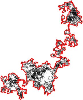
Figure 12: Boundary or outer envelope curve of a planar Brownian path.

In this last part, we are interested in the geometry of the Brownian curve in the plane. By Brownian curve, or Brownian path, we mean the random curve traced by a Brownian motion on the plane. We can see a typical representative in figure 1. In particular, we will consider the boundary of such a curve. It is the outer envelope of the Brownian curve. We observe that it is an extremely irregular curve, fractal in Mandelbrot’s sense (figure 12).

From a series of accurate numerical simulations, Mandelbrot made the conjecture in 1982 that such a boundary is the continuous limit of a particular random walk, the self-avoiding walk (SAW) (figure 13). That is a process where the random walker cannot visit any point of his own path twice. To define it, one considers a priori the ensemble of all possible random paths of a given length (with and without self-intersections) on, say, a square lattice, and select among them the small subset of all the paths that do not self-intersect. Those are then weighted with a uniform measure.

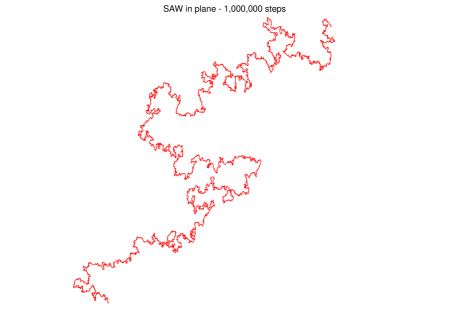
Figure 13: A self-avoiding walk in the plane, made of 1 million steps! (Kindly provided by T. G. Kennedy, University of Arizona.)

The resulting conjecture is that the fractal dimension or Hausdorff dimension of the Brownian boundary is equal to $D_{H}=4/3$, like that which was calculated by the Dutch theoretical physicist Bernard Nienhuis in 1982 for a two-dimensional self-avoiding random walk. The fractal dimension $D_{H}$ is here defined in an non-rigorous way, as follows. We cover the fractal object of size $R$ by small disjoint disks of radius $\varepsilon$, and we count the number $n$ of these disks. In general, this number grows with a power law in $R$ and $\varepsilon$, $n\propto\left(R/\varepsilon\right)^{D_{H}}$. We then see that $D_{H}$ generalizes the notion of Euclidean dimension of regular sets to the case of very irregular sets.

Nienhuis used a representation of statistical mechanics, known as the Coulomb gas, a precursor to the methods of conformal invariance or of conformal field theories that in 1984 would enter the theory of two-dimensional critical phenomena, thanks to the work of Belavin, Polyakov, and Zamolodchikov.

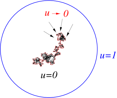
Figure 14: Dirichlet problem associated to a planar Brownian path. The latter serves as an electrode where the potential vanishes.

It was already envisioned in the mid-eighties that the critical properties of planar Brownian paths, whose conformal invariance was well-established, could be the opening gate to rigorous studies of two-dimensional critical phenomena, as advocated in particular by Michael Aizenman. A family of exponents $\zeta_{n}$, governing the non-intersection properties of $n$ Brownian paths, played a crucial role. They are defined as follows: Let $B_{1}(t),B_{2}(t),\cdots$ be independent planar Brownian motions started from distinct points at $t=0$. Then the probability $P_{n}(t)$ that their traces, $B_{1}([0,t]),\cdots,B_{n}([0,t])$, are disjoint is scaling as $t^{-\zeta_{n}}$ as $t\to+\infty$ for constant exponents $\zeta_{n}$.

The precise values of these exponents were originally conjectured in 1988 from conformal invariance and numerical studies. They correspond to a conformal field theory with “central charge” $c=0$. The planar intersection exponents $\zeta_{n}$, for $n\geq 2$, are given by

$$\zeta_{n}=\frac{4n^{2}-1}{24}\,.$$ (127)

Interestingly enough, however, their analytic derivation resisted attempts by standard “Coulomb-gas” techniques, which proved successful for self-avoiding walks, but not for simple walks. A derivation of these Brownian intersection exponents $\zeta_{n}$ (and a heuristic demonstration of Mandelbrot’s related conjecture), inspired by some probabilistic structure of conformal invariance obtained in the meantime by Lawler and Werner, was given by the author in 1998 in the framework of theoretical physics, by means of the formalism of “2D quantum gravity” in conformal field theory.

The same results for the Brownian intersection exponents and Mandelbrot’s conjecture were at last rigorously proved in the framework of probability theory in 2000 by Greg Lawler, Oded Schramm and Wendelin Werner, by means of a conformally invariant stochastic process invented by Schramm, the “$SLE$” (“Stochastic Loewner Evolution”), which is itself based on Brownian motion. Despite the simplicity of formula (127), prior to SLE, its proof by conventional probabilistic techniques had been out of reach.

W. Werner has been awarded the Fields Medal on August 22nd, 2006, at the International Congress of Mathematicians in Madrid,“for his contributions to the development of stochastic Loewner evolution, the geometry of two-dimensional Brownian motion, and conformal field theory.”

We are not going to describe this work in detail here, but we will look instead at the generalization of the results on the geometry of Brownian motion, and at the multifractal nature of its boundary. The latter actually reveals a structure made of a continuum of fractal subsets that we will describe.

In continuity with the previous part, we will focus on the potential theory associated with the neighborhood of a planar Brownian path. We will show how the fine geometry of the Brownian boundary appears as an essential component of the solution to the Dirichlet associated electrostatic problem.

4.2 Potential theory in the neighborhood of a Brownian curve

4.2.1 Brownian Dirichlet problem

Let us then consider a planar Brownian path $\mathcal{B}$ enclosed by a large circle, and the associated Dirichlet problem where the potential $u$ has the value $u=0$ on the boundary $\partial\mathcal{B}$ of the Brownian curve, and $u=1$ on the circle (figure 14). The Brownian path serves as an electrode creating the potential, and by electrostatic induction, its boundary will charge itself. This a priori appears as a rather complex problem, since the Brownian curve is completely random!

Far from the Brownian curve, the potential will depend on the global geometry of the system, and in particular on the presence of the outer circle that acts as an external electrode. Let us imagine for a moment that this circle is pushed towards infinity. Seen from intermediate regions located very far from the Brownian curve (and from the outer circle), the Brownian electrode would then appear to be confined to a point. Its potential will then coincide with that of a point charge equal to the total charge carried by the boundary of the Brownian curve, i.e., the logarithmic Newtonian potential $u_{2}(r)$ (97).

On the other hand, close to the Brownian curve, the geometry of the boundary is crucial. The potential vanishes exactly on the boundary $\partial\mathcal{B}$, and the natural question here is its analytic behavior in the neighborhood of $\partial\mathcal{B}$, i.e., the way in which it goes to $0$. As the geometry of the boundary is particularly wild, the way the potential vanishes is as well.

However, the random Brownian curve hides at its heart a fundamental structural regularity connected to its conformal invariance, and one can in fact describe the potential close to the Brownian path in a way which is probabilistic, but universal.

4.2.2 Conformal invariance

A conformal map $\Phi$ of the plane is a bijection of the plane into itself that preserves angles between curve intersections. To any analytic function $\Phi(z)$ in the complex plane can be associated one such conformal map. Locally, i.e., infinitesimally close to the image $\Phi(z)$ of any point $z$ in complex coordinates, a conformal map is the composition of a local dilation (by a factor of $|\Phi^{\prime}(z)|$), and of a rotation around $\Phi(z)$ (by an angle $\arg\Phi^{\prime}(z)$). This is why angles are locally conserved.

Let us come back for a moment to the Brownian representation of the general Dirichlet problem in a domain $\mathcal{D}$ (figure 11). An auxiliary Brownian motion issued from an arbitrary point $P$, stops upon touching the boundary $\partial\mathcal{D}$, and its Wiener integral represents the potential $u(P)$. Let us imagine the domain $\mathcal{D}$ to be transformed by a conformal map $\Phi$ into a domain ${\mathcal{D}}^{\prime}=\Phi(\mathcal{D})$, while the Brownian trajectory $\mathcal{B}$ is transformed into a curve $\Phi(\mathcal{B})$, which is thus stopped upon touching the boundary $\partial{\mathcal{D}}^{\prime}=\Phi(\partial\mathcal{D})$. Paul Lévy showed that $\Phi(\mathcal{B})$ is still the trajectory of a Brownian motion, after a time reparameterization: this is the property of conformal invariance of planar Brownian motion.

Let us then consider the new potential $u^{\prime}(P^{\prime})$ at a transformed point $P^{\prime}=\Phi(P)$, i.e., the solution to the Dirichlet problem in the transformed domain $\mathcal{D}^{\prime}$. Since all geometric objects that represent the potential were transformed by $\Phi$, and since the transformed auxiliary Brownian path is still Brownian, the result is that its Wiener integral, $u^{\prime}(P^{\prime})$, does not change. The potential $u^{\prime}(P^{\prime})$ is then equal to the potential $u(P)$, that is the solution to the Dirichlet problem in the original domain $\mathcal{D}$, and thus there is an invariance of potential under a conformal map.

In the case we are focusing on here, that is of the Dirichlet problem of a potential $u(P)$ in the neighborhood of a planar Brownian curve (figure 14), the Brownian representation of the potential introduces a second auxiliary Brownian motion that diffuses from the point $P$, while avoiding the original Brownian curve (figure 15). As we just saw, the two Brownian paths are statistically conformally invariant and this probabilistic geometric problem is invariant under any conformal map in the plane.

4.2.3 The role of angles

Conformal maps preserve angles in the plane, and this is why the latter will play an essential role in the description of the potential close to the Brownian boundary.

Let us first consider the simple problem of a potential existing in an angular sector of the plane. More precisely, let us consider an open angle $\theta$ centered at a point $w$ (figure 16). One easily shows, by using the singular conformal map of the complex plane that opens the angle $\theta$ into a flat angle, $\Phi(z)=z^{\pi/\theta}$, that the potential $u(z)$ varies at any point $z$ close to $w$ like

$$u(z)\approx r^{\pi/\theta},$$ (128)

where $r$ is the distance from $w$, $r=|z-w|$. For a flat angle, $\theta=\pi$, and we again find a linear behavior as a function of the distance, corresponding to a constant electric field close to a straight line.

4.3 Multifractality

4.3.1 Distribution of potential

Let us come back finally to the initial question of the distribution of the potential in the region close to a Brownian curve $\mathcal{B}$ (figures 14 and 15). Its boundary $\partial\mathcal{B}$ is a fractal curve without a microscopic scale, and the irregularities of this curve go down to the infinitesimally small. Among all these irregularities, it is natural, from the point of view of potential theory and of conformal invariance, to look for those that are locally like “angles”. Actually, such a distribution of angles and the distribution of the associated potential are invariant under a conformal map. They are then stable in the class of all Brownian curves which are obtained by conformal maps of a single realization of a Brownian curve.

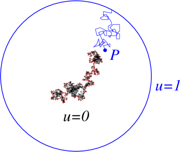
Figure 15: The Dirichlet potential $u$ created at point $P$ by a Brownian curve (center), and vanishing on the boundary of the latter, is represented by a second auxiliary Brownian motion, that diffuses from $P$ towards the exterior, while completely avoiding the first motion.

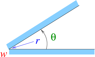
Figure 16: Angular sector with apex $w$ and angle $\theta$.

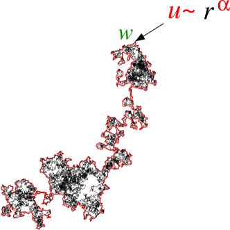
Figure 17: Singular behavior in $r^{\alpha}$ of the potential close to a point $w$ of type $\alpha$.

We can then classify the points $w$ of the boundary $\partial\mathcal{B}$ according to the properties of variation of the potential $u(z)$ when a point $P$ with complex coordinate $z$ approaches $w$ on the boundary. We say that a point $w$ is of type $\alpha$ if

$${u}\left(z\to w\right)\approx r^{\alpha},$$ (129)

in the limit where the distance $r=|z-w|\to 0.$ (Figure 17.)

By comparing the property (129) to the form (128) of the potential of an angle, we see that an exponent $\alpha$ corresponds, from the point of view of the potential, to an equivalent electrostatic angle $\theta$ such that

$$\alpha=\frac{\pi}{\theta}.$$ (130)

The behavior is as if an angle $\theta=\pi/\alpha$ existed locally on the boundary. The angular domain being such that $0\leq\theta\leq 2\pi$, the domain of the exponents $\alpha$ is $1/2\leq\alpha<\infty$, which is rigorously supported by a theorem of A. Beurling. The domain where $\alpha$ is close to $1/2$ corresponds to $\theta$ close to $2\pi$, which is a completely open angular sector, and thus to the presence of an extremely thin needle on the boundary. The domain where $\alpha$ is very large corresponds to $\theta$ close to $0$, thus to a very narrow angular sector, and one then speaks of a fjord.

Now, let ${\partial\mathcal{B}}_{\alpha}$ be the set of points of type $\alpha$ on the boundary. To measure the probability of finding such points of type $\alpha$, we introduce the Hausdorff dimension of the set ${\partial\mathcal{B}}_{\alpha}$,

$$f\left(\alpha\right)={\rm dim}\left({\partial\mathcal{B}}_{\alpha}\right).$$ (131)

This defines the multifractal spectrum $f\left(\alpha\right)$ of the potential distribution. Such a spectrum is conformally invariant in two dimensions, because in any conformal map the local exponents $\alpha=\pi/\theta$ of the potential are themselves invariant.

From a historical point of view, the concept of multifractality was introduced by B. Mandelbrot in 1974, in the context of the phenomenon of turbulence in hydrodynamics, then by H. Hentschel, I. Procaccia, U. Frisch and G. Parisi. It was then further developed at the University of Chicago by T .C. Halsey et al. It corresponds to the existence of a continuous set of fractal dimensions $f(\alpha)$, that are functions of a continuum of exponents $\alpha$.

4.3.2 The Brownian multifractal spectrum

One of the first properties is that the global Hausdorff dimension of a multifractal object is always the maximum of its multifractal spectrum. Thus, for the boundary of a Brownian curve,

$$D_{H}=\sup_{\alpha}f(\alpha)=\frac{4}{3},$$ (132)

because of Mandelbrot’s conjecture, which we mentioned above.

The complete spectrum $f(\alpha)$ for the Brownian curve was calculated in 1998 by a method called “quantum gravity”. One uses a representation of the same problem on a random surface where the metric fluctuates, instead of the normal Euclidean plane. The geometric and probabilistic laws are largely simplified by the “quantum” fluctuations of the metric, and the singular behavior of the Brownian Dirichlet problem is directly accessible!

Next, one can obtain the multifractal spectrum in the plane $\mathbb{R}^{2}$, thanks to a fundamental relationship between critical exponents in the plane and on a random surface, a formula known by the initials “KPZ,” discovered originally in 1988 by three Russian physicists, V. G. Knizhnik, A. M. Polyakov, and A. B. Zamolodchikov. We do not have space here to further develop this method.

We find the formula

$$f(\alpha)=\alpha+b-\frac{b\alpha^{2}}{2\alpha-1},\,\,\,\,\,\,b=\frac{25}{12}.$$ (133)

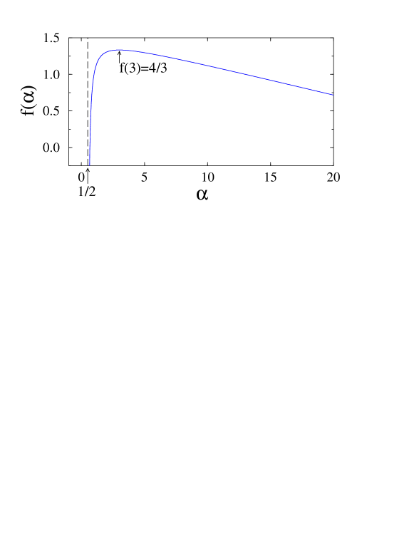
Figure 18: Multifractal function $f(\alpha)$ of the Brownian frontier.

This curve is drawn in figure 18. The definition domain is the half-line $(1/2,+\infty)$. One verifies that the maximum of $f$ is at $4/3$, in agreement with Mandelbrot’s conjecture (132) for the fractal dimension of the boundary. It corresponds to a value of $\alpha=3$, or to a typical electrostatic angle of $\pi/3$.

Moreover, one can calculate by the same method the multifractal spectrum of the potential close to a self-avoiding random walk, and one finds a spectrum which is identical to that of a Brownian curve, fully confirming the identity of the Brownian frontier to a self-avoiding walk in the scaling limit.

One also predicts by this heuristic method that the spectra of a Brownian curve and of a critical percolating cluster are identical. It then follows that both the Brownian frontier and the external perimeter of a critical percolation cluster coincide with the scaling limit of a self-avoiding walk, which further extends Mandelbrot’s conjecture.

Let us mention that the works of Lawler, Schramm, and Werner contain also in principle the necessary information to calculate the spectrum of a Brownian potential. In a rigorous approach using SLE, these authors identify the boundary with that of the ${\rm SLE}_{6}$ process, conjectured also to be an ${\rm SLE}_{8/3}$ and the scaling limit of a self-avoiding polymer.

This curve $f(\alpha)$, also called the harmonic measure spectrum, then solves the problem of the potential distribution close to a Brownian path in a probabilistic sense, since it gives the fractal dimension of the set of points where the potential varies in a specific way, namely as $r^{\alpha}$.

Other values of $b$ in (133) ($b=\frac{25-c}{12}\geq 2$, where $c\leq 1$ is the “central charge” of the associated conformal theory) generate the multifractal spectra of the potential or harmonic measure of conformally invariant random curves in the plane. These are the SLEs describing the boundaries of critical clusters in two-dimensional statistical models, such as Ising or Potts models. For an ${\rm SLE}_{\kappa}$, with $0\leq\kappa<\infty$, one simply sets in (133)

$$c=\frac{1}{4}(6-\kappa)\left(6-\frac{16}{\kappa}\right),\;\;\;\;{b}=1+\frac{1}{8}\left(\kappa+\frac{16}{\kappa}\right).$$ (134)

4.4 Generalized multifractality

4.4.1 Logarithmic spirals

Until now we have considered variations of the potential only. We can also study the form of the equipotential lines. As the potential follows the properties of conformal invariance of the Brownian curve, it is now necessary first to determine the geometric forms that are conserved by such invariance.

These are the logarithmic spirals that play a particular role in potential theory in two dimensions. One such spiral centered at the origin is defined by the logarithmic variation of the polar angle $\varphi$ as a function of the distance $r$ from the origin:

$$\varphi=\lambda\ln\,r\ ,$$

where $\lambda$ is a real positive or negative parameter.

When we apply a conformal map $\Phi$, around the center it is equivalent to a dilation $r\to|\Phi^{\prime}(0)|\,r$, composed with a rotation. The dilation transforms the angle $\varphi=\lambda\ln\,r$ into $\lambda\ln\,r+\lambda|\Phi^{\prime}(0)|$, which thus amounts to a local rotation of the spiral, whose geometrical shape is thereby locally conserved.

In the potential theory considered here, the Brownian frontier is equipotential by construction. There exists a multitude of points where such equipotential boundary will locally roll onto itself in a double logarithmic spiral, as shown in figure 19.

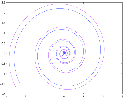
Figure 19: Double logarithmic spiral.

4.4.2 Mixed multifractal spectrum

We come then to Ilia Binder’s idea from his thesis in 1997 defining a generalized multifractality. One looks for a set ${\partial\mathcal{B}}_{\alpha,\lambda}$ of points $w$ of the boundary ${\partial\mathcal{B}}$, where the potential varies like $r^{\alpha}$, and the boundary spirals at a given rate $\lambda$. These conditions can be heuristically written for a point $z$ close to $w$:

$${u}\left(z\to w\in{\partial\mathcal{B}}_{\alpha,\lambda}\right) \approx r^{\alpha},$$

$$\varphi\left(z\to w\in{\partial\mathcal{B}}_{\alpha,\lambda}\right) \approx \lambda\ln\,r\ ,$$ (135)

in the limit $r=|z-w|\to 0$. The Hausdorff dimension $f\left(\alpha,\lambda\right)={\rm dim}\left({\partial\mathcal{B}}_{\alpha,\lambda}\right)$ then defines the mixed multifractal spectrum, which is conformal invariant because under a conformal map both $\alpha$ and $\lambda$ are locally invariant.

With Ilia Binder, we computed such a mixed spectrum for a Brownian motion, by the quantum gravity method. It satisfies an exact scaling law

$$f(\alpha,\lambda)=(1+\lambda^{2})f\left(\frac{\alpha}{1+\lambda^{2}}\right)-b\lambda^{2}\ ,$$ (136)

which gives from (133)

$$f(\alpha,\lambda)=\alpha+b-\frac{b\alpha^{2}}{2\alpha-1-\lambda^{2}},\,\,\,\,\,\,b=\frac{25}{12}.$$ (137)

Its domain of definition is ${\alpha}\geq\frac{1}{2}({1+\lambda^{2}})$, according to a theorem of Beurling. Different spectra are represented in figure 20.

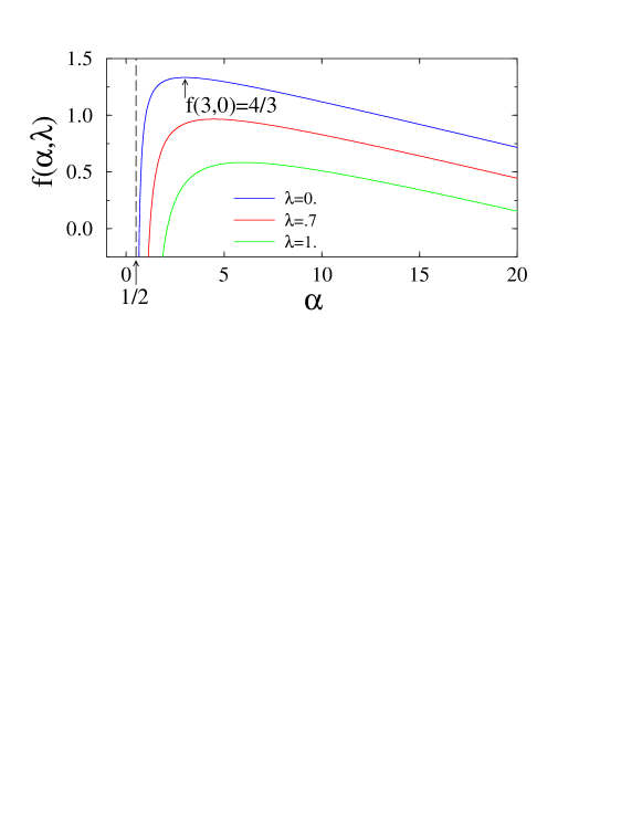
Figure 20: Universal multifractal spectrum $f(\alpha,\lambda)$ of a Brownian path for different values of spiral rate $\lambda$. The maximum $f(3,0)=4/3$ is the Hausdorff dimension of the Brownian frontier.

Since this function does not depend on the sign of $\lambda$, spiral rotations in positive and negative directions are equiprobable, as expected. One recovers the harmonic spectrum $f(\alpha)$ as the maximum

$$f(\alpha)=f(\alpha,\lambda=0)={\sup}_{\alpha}f(\alpha,\lambda).$$

By symmetry, the most probable situation for a point on the boundary is the absence of spiral rotation, i.e., $\lambda=0$.

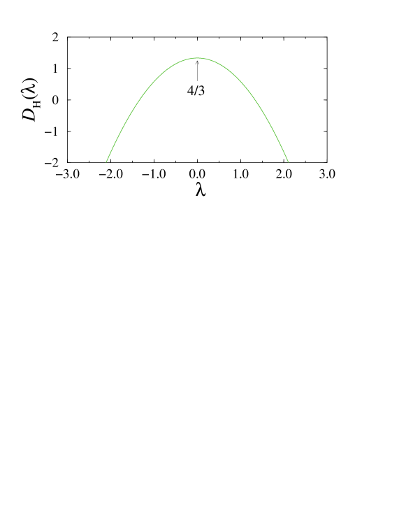
Figure 21: Fractal dimension $D_{H}(\lambda)$ of spirals of type $\lambda$ along the Brownian boundary.

One can then also consider only the fractal dimension $D_{H}(\lambda)$ of the points on the boundary, which are the tips of logarithmic spirals of type $\lambda$. For this, we take the maximum of the mixed spectrum with respect to the other variable, $\alpha$:

$$D_{H}(\lambda)={\sup}_{\alpha}f(\alpha,\lambda)=\frac{4}{3}-\frac{3}{4}\lambda^{2}.$$

This fractal dimension then has the form of a parabola as a function of $\lambda$, whose maximum is still the global Hausdorff dimension of the boundary, $D_{H}=4/3$ (figure 21).

Let us add a few final remarks.

The quantum gravity calculations can be generalized to the whole class of conformally invariant curves on the plane, and to Schramm’s SLE process. The spectra are given by the same formulae (133) and (137) for different values of the parameter $b$. For the ${\rm SLE}_{\kappa}$ process, one substitutes:

$${b}=1+\frac{1}{8}\left(\kappa+\frac{16}{\kappa}\right)=\frac{1}{2\kappa}\left(2+\frac{\kappa}{2}\right)^{2},\;\;\kappa\in\mathbb{R}^{+}.$$

Lastly, these multifractal results, originally found heuristically in theoretical physics, can in principle be rigorously proved in the general probabilistic framework of ${\rm SLE}_{\kappa}$. The application of this general result to the case of the Brownian and percolation cluster frontiers is then obtained by identifying those boundaries to that of the ${\rm SLE}_{6}$ process (thanks to works by Lawler, Schramm, and Werner and also by S. Smirnov, and V. Beffara), while, from a rigorous point of view, the similar identification of the scaling limit of a self-avoiding walk to a ${\rm SLE}_{8/3}$ process, although certainly true, remains to be proven!

Here we pause in 2005 at the end of the path started in 1827 by Robert Brown with his observations at the microscope, and by Einstein in 1905 with his theory of Brownian fluctuations. The new paradigm of stochastic paths could be today the SLE, or Stochastic Loewner Evolution, generated itself by Brownian motion on the boundary of a planar domain, and its rather extraordinary conformal invariance properties in the Euclidean plane. This process brought us to the shores of two-dimensional quantum gravity, where the SLE stochasticity seems to call for fluctuations of the metric, hence “quantum gravity.” In some sense, we are brought back to the work of Einstein, whose 1916 general relativity theory explained how gravitation is equivalent to a change of metric. Now it is Statistical Mechanics that stands in the breach, let us wish for fruitful developments!

Acknowledgements:

I would like to thank John Stachel, Editor of the Complete Papers of Albert Einstein, for his kind permission to reproduce some material of the Editorial Notes.

I thank Bruce H. J. McKellar and Rod W. Home for kindly providing first-hand information regarding the work of W. Sutherland, and Hector Giacomini for information about the Besso-Einstein correspondence. I also wish to thank Jean-Pierre Kahane for stimulating exchanges about R. Brown and A. Brongniart, Giovanni Gallavotti about G. Cantoni, as well as André Rougé about L. Bachelier. I also thank Christian Van den Broeck and Chris Jarzynski for providing up-to-date information about their latest works, and for interesting discussions about Brownian motion, the Maxwell demon and the second principle.

I wish to thank Emmanuel Guitter for creating the figures, and Michel Bauer, Denis Bernard, Vincent Pasquier, and Jean-Louis Sikorav for useful comments.

Special thanks go to Thomas C. Halsey, David Kosower, Robert S. MacKay, Kirone and Shamlal Mallick, and Larry S. Schulman for their careful and critical proofreading of this article, to Thomas C. Halsey for introducing me to the concept of multifractality almost 20 years ago, and to Kirone Mallick and Ugo Moschella for their precious help during the completion of this article.

Last, but not least, I wish to express my gratitude to Emily Parks (and to Graziano Vernizzi!) who carried out the redoubtable task of translating the original text from French into English.

Bertrand Duplantier
Service de Physique Théorique
Orme des Merisiers
CEA/Saclay
F-91191 Gif-sur-Yvette Cedex, France
e-mail: Bertrand.Duplantier@cea.fr