Polaronic features in the optical properties of the Holstein-$t$-$J$ model

Abstract

We derive the exact solution for the optical conductivity $\sigma(\omega)$ of one hole in the Holstein-$t$-$J$ model in the framework of dynamical mean-field theory (DMFT). We investigate the magnetic and phonon features associated with polaron formation as a function of the exchange coupling $J$, of the electron-phonon interaction $\lambda$ and of the temperature. Our solution directly relates the features of the optical conductivity to the excitations in the single-particle spectral function, revealing two distinct mechanisms of closing and filling of the optical pseudogap that take place upon varying the microscopic parameters. We show that the optical absorption at the polaron crossover is characterized by a coexistence of a magnon peak at low frequency and a broad polaronic band at higher frequency. An analytical expression for $\sigma(\omega)$ valid in the polaronic regime is presented.

I Introduction

The problem of a single hole in the $t$-$J$ model interacting also with the lattice degrees of freedom has recently attracted a notable interest in connection with the physical properties of the high-$T_{c}$ cuprates. mish1 ; rosch1 ; rosch3 ; gunn ; prev In particular, in parent and strongly underdoped compounds, angle resolved photoemission spectroscopy (ARPES) reveals a low energy peak whose dispersion is well described by the $t$-$J$ model, while its anomalously large broadness has been ascribed to incoherent multi-phonon shake-off processes.shen ; shen2 ; mish1 ; rosch3 A similar interplay between electron-electron and electron-phonon interactions should in principle be reflected in the optical conductivity spectra. As a matter of fact, the most remarkable features observed in the underdoped region are an ubiquitous mid-infrared (MIR) peak at $\approx 0.5$ eV, and a weaker peak around $\approx 0.1$ eV, the latter being more strongly doping and temperature dependent.MIR-review ; MIR-review2 Several interpretations have been proposed for the origin of these features, including midgap or impurity states, impurityMIR1 ; impurityMIR2 charge/spin stripes,stripesMIR ; stripesMIR2 polaronic excitations,polaronMIR ; polaronMIRb ; polaronMIR2 ; polaronMIR3 ; polaronMIR4 and the interaction with the antiferromagnetic background.impurityMIR2

The first proposal of the $t$-$J$ model as a suitable basis to discuss the optical spectra of the cuprates was advanced by Zhang and Rice zr who observed that the $1/\omega$ behaviortimusk of the optical absorption above $\approx 0.5$ eV could be naturally associated to the incoherent motion in an antiferromagnetic background. Successively, the optical conductivity of the $t$-$J$ model has been investigated in detail using several techniques, such as exact-diagonalization,dagotto analytical approximationstikofsky ; bang ; kyung_tJ ; jackeli and dynamical mean-field theory (DMFT).strack ; logan ; jarrell ; haule However, and in spite of the above discussed relevance of the electron-phonon coupling, the optical conductivity of the $t$-$J$ model in the presence of the lattice degrees of freedom has not been thoroughly investigated. Numerical calculations based on exact-diagonalization of finite clusters were employed for instance in Ref. feshke, to evaluate $\sigma(\omega)$. Alternatively, the optical conductivity was calculated analytically in Ref. kyung, based on a non-crossing Born approximation, which is however unable to describe the polaron formation.

In this paper we present results for the optical conductivity of a single hole in the Holstein-$t$-$J$ model obtained in the framework of dynamical mean-field theory. One-hole spectral properties at zero temperature were discussed in a previous publication where antiferromagnetic correlations were shown to enhance the effects of the electron-phonon coupling.cc A similar result was found also in the antiferromagnetic phase of the Holstein-Hubbard model using DMFT techniques.StJAF A serious drawback of DMFT, which is obtained as the exact solution of the lattice problem in the limit of infinite dimensions, is that the magnetic background is treated in a classical way. This, together with the fact that Trugman loops are negligible in infinite dimensions, prevents the possibility to account for coherent hole-propagation, which is related to the spin-flip fluctuations. As a consequence, no Drude peak can be observed in the optical conductivity. On the other hand, the incoherent contributions of $\sigma(\omega)$ are mainly dominated by local properties, such as the local electron-phonon scattering and spin-string excitations within the magnetic polaron, which are well captured by this approach.cc

Bearing the above limitations in mind, the aim of the present work is thus to focus on the incoherent part of the optical conductivity of a single-hole and to investigate in detail its features in the different physical regimes of the Holstein-$t$-$J$ model. The dependence of the optical spectra on the microscopic parameters is analyzed with special attention to the intermediate coupling region, where the interplay between magnetic and lattice degrees of freedom is strongest. We show that a crucial role is played by the formation of the lattice polaron, which drives a transfer of spectral weight towards higher frequencies, opening a pseudogap at low frequencies. Conversely, starting from the polaronic phase, two different mechanisms can be clearly identified as being responsible for the disappearance of the pseudogap: $i$) reducing the effective exchange energy scale suppresses the positive feedback of magnetism on polaron formation and can lead to a closing of the pseudogap as the system crosses back to the non-polaronic regime; $ii$) increasing the temperature, which does not alter the lattice/magnetic interplay, leads to a filling of the pseudogap more similar to what is expected in purely polaronic models. In the immediate vicinity of the polaron crossover, the spectra are characterized by a coexistence of a magnon peak at low frequency and a broad polaronic band at higher frequency, which closely resembles the experimental situation observed in the cuprates.

On theoretical grounds, the definition of the optical conductivity of a single hole is a delicate matter which needs particular care. We provide an analytical derivation which generalizes the results of Refs. logan, ; fratini, to the Holstein-$t$-$J$ model. This approach permits us to identify the role of the different one-particle properties on the optical conductivity. Comparison with numerical data is also discussed, showing a good agreement between our findings and exact diagonalization results.

The paper is organized as follows. In Sec. II we discuss the exact solution in infinite dimensions for the one-hole Green’s function of the Holstein-$t$-$J$ model at finite temperature. Results for the one-particle spectral features are discussed in Sec. III. An analytical expression for the optical conductivity $\sigma(\omega)$ is derived in Sec. IV where we also investigate the different polaronic features and their dependence on the microscopic parameters. In Sec. V we present a further simplified expression for $\sigma(\omega)$ valid in the lattice polaron regime. The main results are briefly summarized in Sec. VI where also the consequences of including spin fluctuations (here neglected) is also discussed. Finally, a detailed derivation of the analytical expression for the one-particle spectral function and the optical conductivity is reported in the Appendices.

II Holstein-$t$-$J$ model in infinite dimensions

In the following we consider the case of a single hole in an antiferromagnetic (AF) background interacting with local Holstein phonons. Using the linear spin-wave approximationmartinez ; ramsak ; marsiglio and neglecting terms that vanish in the limit of large coordination number $z\gg 1$, we can write the Hamiltonian as:cc

$$H = \frac{t}{2\sqrt{z}}\sum_{\langle ij\rangle}\left(h_{j}^{\dagger}h_{i}a_{j}+{\rm h.c.}\right)+\frac{J(1-2x)}{2}\sum_{i}a_{i}^{\dagger}a_{i}+$$ (1)

$$+ g\sum_{i}h_{i}^{\dagger}h_{i}\left(b_{i}+b_{i}^{\dagger}\right)+\omega_{0}\sum_{i}b_{i}^{\dagger}b_{i}.$$

Here $a^{\dagger}$ is the creation operator for boson spin defects, $h^{\dagger}$ is the single spinless hole operator and $x=\langle a^{\dagger}a\rangle$ represents the density of spin defects which is finite at nonzero temperature. Note that in the thermodynamical limit the presence of a single hole does not affect the magnetic state, which can be thus evaluated (in the $z\gg 1$ limit) in the absence of spin dynamics. The density of spin defects can be obtained from the magnetization $m=1-2x$ via the Curie-Weiss equation:

$$m=\tanh\left(\frac{\beta Jm}{4}\right),$$ (2)

which defines a Néel temperature $T_{\rm N}=J/4$. Concerning the electron-lattice interaction, we shall mainly focus on the adiabatic regime $\omega_{0}\ll t$ which is relevant to the experimental systems of interest. In this regime, a dimensionless electron-phonon coupling constant can be defined as $\lambda=g^{2}/\omega_{0}t$, the polaron energy in units of the hopping integral.

An exact solution for the thermodynamical and the one-particle spectral properties of Eq. (1) at $T=0$ was obtained in Ref. cc, in terms of a continued fraction. In order to derive the optical conductivity, the one-particle Green’s function must be generalized to finite temperature, which involves the following steps: $i$) one has to allow for thermally excited phonons; $ii$) the presence of thermally excited spin defects requires the introduction of a “spin-resolved” Green’s function, to distinguish hole excitations created on sites with/without spin defects; $iii$) finally, the reduced magnetization introduces an effective exchange coupling $\tilde{J}=Jm<J$. The details of a formal derivation of the one-particle propagator at finite temperature are reported in Appendix A; we summarize here the main results.

Following Ref. logan, , we define $\bar{G}_{i,0}(\omega)=\bar{G}_{i}(\omega)$ as the Green’s function for one hole created on a site in the absence of spin defects. A careful analysis (see Appendix A) shows that the Green’s function $\bar{G}_{i,1}(\omega)$ for a hole created on a site with a spin defect is simply $\bar{G}_{i,1}(\omega)=\bar{G}_{i}(\omega+J)$. In addition, at finite temperature the Green’s function $\bar{G}_{i}(\omega)$ itself is defined as a thermal average over the phonons:

$$\bar{G}(\omega)=\frac{1}{Z_{\rm ph}}\sum_{n}\mbox{e}^{-\beta n\omega_{0}}\bar{G}^{nn}(\omega+n\omega_{0}),$$ (3)

where $\bar{G}^{nn}(\omega)$ represents the propagation of one hole created on a site with $n$ excited phonons and $Z_{\rm ph}$ is the single-site phonon partition function $Z_{\rm ph}=1/(1-\mbox{e}^{-\beta\omega_{0}})$. Following Ref. polarone, , we can derive a self-consistent expression for $\bar{G}^{nn}$ in terms of a continued fraction. We can write:

$$\bar{G}^{nn}(\omega)=\frac{1}{{\cal G}^{-1}(\omega-n\omega_{0})-\Sigma_{\rm em}^{n}(\omega)-\Sigma_{\rm abs}^{n}(\omega)},$$ (4)

where

$$\Sigma_{\rm em}^{n}(\omega) = \frac{(n+1)g^{2}}{\displaystyle{\cal G}^{-1}(\omega-(n+1)\omega_{0})-\frac{\displaystyle(n+2)g^{2}}{\displaystyle{\cal G}^{-1}(\omega-(n+2)\omega_{0})-\frac{\displaystyle(n+3)g^{2}}{\displaystyle\ldots}}},$$ (5)

$$\Sigma_{\rm abs}^{n}(\omega) = \frac{ng^{2}}{\displaystyle{\cal G}^{-1}(\omega-n\omega_{0})-\frac{\displaystyle(n-1)g^{2}}{\displaystyle{\cal G}^{-1}(\omega-(n-1)\omega_{0})-\frac{\displaystyle(n-2)g^{2}}{\displaystyle\ldots}}}.$$ (6)

Carrier motion and exchange interactions are taken into account by the bath propagator

$${\cal G}^{-1}(\omega)=\omega-\Sigma_{t}(\omega),$$ (7)

where the “hopping” self-energy is defined as

$$\Sigma_{t}(\omega)=\frac{t^{2}}{4}\left[(1-x)\bar{G}_{j}(\omega-\tilde{J}/2)+x\bar{G}_{j}(\omega+\tilde{J}/2)\right].$$ (8)

Finally, the spin-defect averaged Green’s function, which is the physically probed quantity in photoemission experiments, is obtained as:

$$G(\omega)=(1-x)\bar{G}(\omega)+x\bar{G}(\omega+\tilde{J}/2).$$ (9)

Note that the factors $(1-x)$ and $x$ in front of $\bar{G}_{j}(\omega-\tilde{J}/2)$ and $\bar{G}_{j}(\omega+\tilde{J}/2)$ account for the probability of a site to be, respectively, free or populated by a spin defect. Note also that the Green’s function $\bar{G}(\omega)$ appearing in Eqs. (7,8) is a phonon averaged quantity, so that the solution of Eqs. (3)-(9) involves the simultaneous self-consistency of all of the $\bar{G}_{i}^{nn}$, which is much more computationally expensive than the solution at zero temperature.

It is easy to check that in the absence of electron-phonon interaction Eq. (9) recovers the thermal Green’s function for the pure $t$-$J$ model as defined in Eq. (2.12) by Stumpf and Logan.logan On the other hand, it should be stressed that the present solution, although it formally recovers the results for the pure Holstein model in the limit $\tilde{J}\rightarrow 0$ (paramagnetic case) [Eqs. (40)-(42) of Ref. polarone, ], is still described by a purely local Green’s function $G_{i,j}(\omega)=\delta_{i,j}G(\omega)$ due to the assumption of a classical (although disordered) spin background. The main drawback of this assumption is thus that no coherent dispersive peak is obtained in this framework even in the $J\rightarrow 0$ limit of the $t$-$J$ Holstein model, and, consequently, no Drude peak appears in the optical conductivity. Notwithstanding this limitation the present approach, as we will show below, is still quite able to reproduce in more than qualitative agreement the incoherent features of both the one-particle Green’s function and of the optical conductivity.

III One-hole spectral properties

Before discussing the optical conductivity, let us briefly present our results for the one-particle spectral function in the Holstein-$t$-$J$ model at finite temperature. Previous approaches have focused separately on thermal effects either in the pure Holstein or in the pure $t$-$J$ model. The temperature evolution of the hole spectral function $\rho(\omega)=-(1/\pi)\mbox{Im}G(\omega)$ for the $t$-$J$ model in the infinite dimensional limit has been analyzed in Ref. logan, . At $T=0$, it consists of a series of $\delta$-function magnon peaks whose distribution reflects the strength of the magnetic polaron: for sufficiently large $J/t$ the profile is rapidly decaying with energy (reminiscent of the string picture of small magnetic polarons) whereas for small $J/t$ it acquires a more symmetric shape, reducing to a semi-circular function in the limit $J/t\rightarrow 0$. The effect of a non-zero temperature within this context is to broaden each $\delta$-function with a bandwidth $W_{x}$ which is ruled by the thermal spin defect probability $x$. We shall term this effect the intrinsic magnetic broadening. Such intrinsic magnetic broadening $W_{x}$ is however exponentially small for $T/T_{\rm N}\ll 1$, and it becomes significant only close to $T_{\rm N}$. A semi-circular shape is recovered also in the paramagnetic phase $T\geq T_{\rm N}$, where $\tilde{J}/t=0$.

As the electron-lattice coupling is turned on, each magnon peak splits into several sub-peaks spaced by $\omega_{0}$, reflecting the dressing of the hole by phononic excitations. In this context the strength of the electron-phonon coupling rules not only the number of phonon satellites but also its spectral weight profile. Just as in the pure Holstein model, while the number of phonon peaks is quite small in the weak coupling regime, in the polaronic state a large number of phonon satellites appear with a characteristic Gaussian profile. The envelope of the phononic fine structure has a spread which is governed by the energy associated with the lattice fluctuations: it is given by $\sqrt{\lambda\omega_{0}t}=g$ in the quantum limit, and increases $\sqrt{2\lambda Tt}$ as $T\gtrsim\omega_{0}/2$. hohu

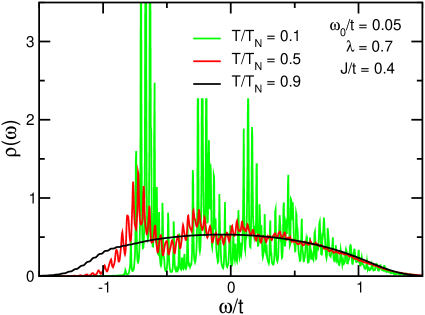
Figure 1: (color online) Temperature evolution of the total spectral function $\rho(\omega)=-(1/\pi)\mbox{Im}G(\omega)$ in the polaronic regime. Microscopical parameters: $\lambda=0.7$, $\omega_{0}/t=0.05$, $J/t=0.4$ and $T/T_{\rm N}=0.1,0.5,0.9$ (corresponding to $T/\omega_{0}=0.2,1,1.8$). Numerical calculations have been done with a small imaginary frequency part $\eta=0.007$.

In Fig. 1 we show the temperature evolution of a typical polaronic spectral function, at $\lambda=0.7$, $\omega_{0}/t=0.05$ and $J/t=0.4$. Throughout the paper, when not specified, we shall take the hopping matrix element $t$ as the energy unit. The temperatures considered here are $T/T_{\rm N}=0.1,0.5,0.9$, corresponding to $T/\omega_{0}=0.2,1,1.8$. At the lowest temperature ($T/T_{\rm N}=0.1$) a phononic fine structure can be clearly seen, superimposed on the magnon peaks. The width of each phononic peak is due to the intrinsic magnetic broadening $W_{x}$ described in Ref. logan, . It is exponentially small at this temperature, so that a small Lorentzian broadening $\eta=0.007$ has been introduced for clarity. On the other hand, the spread of the multiphonon structure gives rise to an overall width to the magnon peaks that is in good agreement with the expected value $g=0.19$.

Upon increasing the temperature to $T/T_{\rm N}=0.5$, two different effects are visible. First, the width $W_{x}$ of each of the fine peaks increases due to the intrinsic magnetic broadening, leading to a much smoother curve (this effect actually overcomes the small Lorentzian broadening $\eta$ introduced previously). Also, the overall spread of the multiphonon profiles increases due to the thermal phonon fluctuations, as expected for $T\gtrsim\omega_{0}/2$. Finally, at $T/T_{\rm N}=0.9$, the system is so close to the paramagnetic phase that neither the phonon peaks nor the magnon structure can be resolved.

At this point, it is useful to comment about the effects of coherent hole propagation, that are implicitly neglected in our approach. These would induce a finite dispersion of order $\sim J$ to the lowest energy magnon peak.mish1 ; feshke ; kyung ; martinez ; kane ; marsiglio It is clear that such dispersion would be visible only at sufficiently low temperatures and at moderate electron-phonon coupling strengths, when the energy scale $J$ is smaller than both the intrinsic magnetic broadening and the Gaussian phonon spread, whereas in the opposite case it will presumably be hidden below a featureless background. These considerations give further support to the present DMFT approach in the polaronic and/or high temperature regime, where neglecting the coherent hole propagation would not affect significantly the spectral properties. As we shall see below, this is even more true for what regards the finite-frequency optical conductivity, where any dispersive peak would be convolved in any case with high-energy featureless structures.

IV Optical conductivity

The evaluation of the optical conductivity for a single hole is a delicate matter, which is only partly simplified in the context of DMFT due to the absence of vertex corrections.khurana A controlled procedure is derived in terms of an expansion of the inverse fugacity at finite temperature, performing the limit $\mu\rightarrow-\infty$ to enforce the thermodynamically vanishing particle density. We can thus define the optical conductivity per hole, $\sigma(\omega)=\lim_{n_{h}\rightarrow 0}\sigma(\omega;n_{h})/n_{h}$, which is a finite quantity and which presents the same features as in the dilute (but finite) hole density limit. Applying this formalism one derives a similar expression as obtained in Refs. zr, ; logan, , here adapted to take into account the electron-phonon interaction. Leaving once more the technical details in Appendix B, we report here the main results. The optical conductivity per hole is expressed as

$$\sigma(\omega) = \frac{t^{2}\pi(1-\mbox{e}^{-\beta\omega})}{4\omega}\int d\Omega\,\bar{\rho}^{\rm w}(\Omega)$$ (10)

$$\times\left[x\bar{\rho}(\omega+\Omega+\tilde{J}/2)+(1-x)\bar{\rho}(\omega+\Omega-\tilde{J}/2)\right],$$

where

$$\bar{\rho}(\omega) = -\frac{1}{\pi}\mbox{Im}\bar{G}(\omega),$$ (11)

and

$$\bar{\rho}^{\rm w}(\omega) = \frac{\mbox{e}^{-\beta\omega}\bar{\rho}(\omega)}{\int d\omega\,\mbox{e}^{-\beta\omega}\bar{\rho}(\omega)}.$$ (12)

The last line defines a “weighted spectral function”, $\bar{\rho}^{\rm w}(\omega)$, which represents thermally excited states and plays an important role in the determination of the optical conductivity.

Let us remark that, although Eqs. (10)-(12) are formally analogous to those for the pure $t$-$J$ model, the electron-phonon interaction appears implicitly in them in the evaluation of the local Green’s function $\bar{G}(\omega)$. Note also that, in the paramagnetic limit $\tilde{J}\rightarrow 0$, Eqs. (10)-(12) do not recover the results of the Holstein model,fratini because Eq. (10) involves the convolution of two local rather than k-dependent propagators. As discussed above, this is due to the classical treatment of the spin degrees of freedom which does not allow for coherent transport, so that no Drude peak is recovered in the present analysis. This, however, has only a minor influence on the finite-frequency optical conductivity, which is dominated by local incoherent excitations.

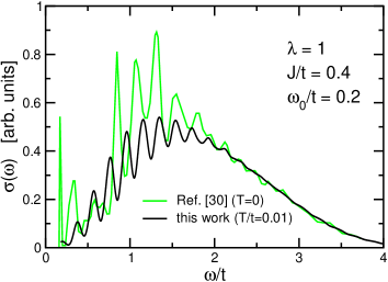
Figure 2: (color online) Comparison between the optical conductivity $\sigma(\omega)$ obtained by our DMFT solution and Lanczos diagonalization in two dimensions on a finite cluster (Ref. feshke, , arbitrarily scaled). A Gaussian broadening $\Delta=3\omega_{0}/5$ for $\sigma(\omega)$ has been employed in our DMFT analysis (see text for details).

In order to assess the validity of the present treatment, we compare in Fig. 2 the optical conductivity of the Holstein-$t$-$J$ model in infinite dimensions, as described by Eqs. (10)-(12), with numerical calculations using Lanczos diagonalization for a single hole in the 2D Holstein-$t$-$J$ model on a $\sqrt{10}\times\sqrt{10}$ cluster.feshke For technical reasons (see discussion below), DMFT data are averaged with a Gaussian filter of amplitude $\Delta=3\omega_{0}/5$ such that phonon resonances are still well separated. Microscopic values are $\lambda=1$, $J/t=0.4$, $\omega_{0}/t=0.2$, and $T=0$ (for Ref. feshke, ) and $T=0.01t=0.1T_{\rm N}$ for the present results. These values correspond to a case where the lattice/magnetic polaron is formed and incoherent contributions to the optical conductivity are indeed dominant. The good agreement of the overall shape confirms the feasibility of our analysis to investigate the finite frequency optical conductivity.

IV.1 Technical details

As discussed in the previous Section, the one-hole spectral function consists of a set of narrow bands whose width $W_{x}$ is controlled by the intrinsic magnetic broadening. This intrinsic width vanishes at low temperature due to the absence of spin-wave dispersion, making the direct evaluation of Eqs. (10)-(12) quite hard to perform. Special care is thus needed in order to calculate numerically the optical conductivity.

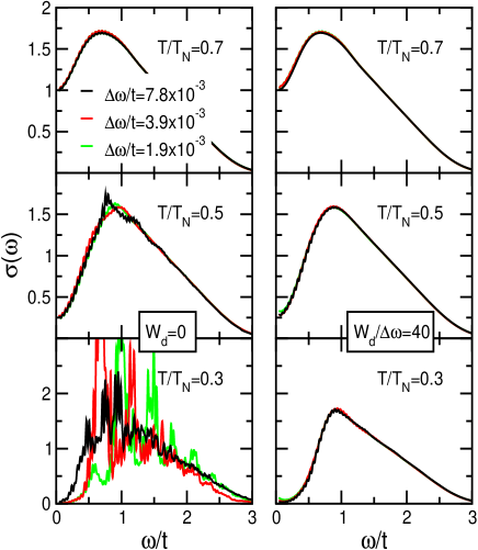
Figure 3: (color online) Left panels: Gaussian averaged optical conductivity as a function of the sampling mesh $\Delta\omega$ for different temperatures. Right panel: the corresponding Gaussian averaged optical conductivity in the presence of a disorder-induced bandwidth $W_{d}/\Delta\omega=40$ as described by our scaling procedure. The microscopic parameters are $\lambda=0.7$, $\omega_{0}/t=0.05$ and $J/t=0.4$.

We shall be mainly interested in the features of the optical conductivity that are related to the electron-lattice coupling. We shall therefore retain the details of the spectra on the scale of the phonon frequency $\omega_{0}$. From the practical point of view, the primary object of our analysis will be a Gaussian average of the optical conductivity $\sigma(\omega)$ with a Gaussian filter of amplitude $\Delta=3\omega_{0}/5$.notagaux Note that, even though the Gaussian average preserves the total spectral weight of the original set of data, the accuracy of the final result will be limited by the finite frequency sampling $\Delta\omega$. In explicit terms, if the spacing $\Delta\omega$ is larger than the intrinsic peak-width $W_{x}$, the data sampling will probe the spectral features in a random way, yielding a highly inaccurate result for both the shape and spectral weight of the optical conductivity. This is shown in the left panels of Fig. 3 where we plot the dependence of the (Gaussian averaged) optical conductivity on the sampling spacing $\Delta\omega$ for different temperatures. At high temperature $T/T_{\rm N}=0.7$ the intrinsic magnetic broadening $W_{x}$ is large enough so that both the shape and the total spectral weight of the optical conductivity are well captured even with a relatively large mesh ($\Delta\omega/t=7.8\times 10^{-3}$). At lower temperature $T/T_{\rm N}=0.5$ however $W_{x}$ becomes so small that a much finer mesh ($\Delta\omega/t=1.9\times 10^{-3}$) is needed in order to get accurate results. At $T/T_{\rm N}=0.3$, finally, no convergence is achieved even for the finest sampling mesh considered in this paper, $\Delta\omega/t=1.1\times 10^{-4}$ (in Fig. 3, for graphical reasons, we plot curves only up to $\Delta\omega/t=1.9\times 10^{-3}$). Clearly, since the intrinsic peak-width $W_{x}$ vanishes exponentially at low $T$, the problem evidenced here cannot be solved by merely reducing the sampling mesh.

To overcome this difficulty we add to the system a small uncorrelated disorder with semielliptic distribution of amplitude $W_{d}$,strack ; logan which is able to yield a finite peak-width even in the zero temperature limit. We choose $W_{d}=40\Delta\omega$ to assure a sufficiently dense mesh for an accurate sampling. We then scale $W_{d}\rightarrow 0$ keeping fixed the ratio $W_{d}/\Delta\omega=40$ in order to approach the correct physical limit in the absence of disorder. Results obtained with a finite $W_{d}$ are shown in the right panels of Fig. 3. No appreciable difference is visible at high temperature $T/T_{\rm N}=0.7$ where the thermally driven magnetic broadening $W_{x}$ is large enough to guarantee the convergence even in the absence of disorder. On the other hand our procedure provides a clear improvement already at $T/T_{\rm N}=0.5$ where the convergence as function of the sampling spacing is more easily achieved in the presence of disorder (note that the converged results coincide with the results for the most dense mesh in the absence of disorder, showing that no spurious structures appear due to our scaling procedure). Finally, for $T/T_{\rm N}=0.3$ the disorder scaling procedure is the only way to guarantee convergence of both the shape and the total spectral weight of the optical conductivity.

IV.2 Results

Using the above described procedure, we shall now concentrate on the evolution of the optical conductivity in the adiabatic regime, fixing the ratio $\omega_{0}/t=0.05$. This value is qualitatively representative of the cuprates, where the half-bandwidth $t\approx 1.2$ eV and typical optical phonon frequencies $\omega_{\rm ph}\approx 60$ meV. This regime is also the most interesting one from the theoretical point of view, since in this case the interplay between lattice and spin degrees of freedom has its most dramatic effects.

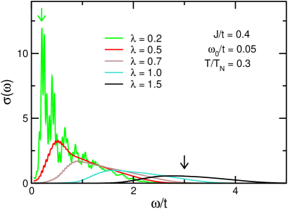
Figure 4: (color online) Optical conductivity versus $\lambda$ across the polaron crossover, at fixed $J=0.4$, $\omega_{0}/t=0.05$ and $T/\omega_{0}=0.6$ ($T/T_{N}=0.3$). The two arrows at low and high energy mark respectively the first magnon peak at $\omega\approx J/2$ in the weak electron-phonon coupling limit $\lambda\ll 1$, and the position $\omega\approx 2\lambda t$ of the broad polaronic absorption expected at $\lambda\gg 1$ (shown here for $\lambda=1.5$).

Fig. 4 shows the evolution of the optical absorption at fixed $J/t=0.4$ and low temperature $T/T_{N}=0.3$, upon varying the electron-lattice coupling. At $\lambda=0.2$, the result is very reminiscent of the spectra calculated for the pure $t$-$J$ model in Ref. logan, . It consists of a series of magnetic peaks, dominated by the sharp single-magnon peak located at $\omega\simeq J/2$ and rapidly decaying at higher frequency. In this weak-coupling regime $\lambda=0.2$, the electron-phonon interaction simply gives rise to a multi-phonon fine-structure with a Gaussian profile. Each magnon peak acquires thus a phonon-driven width without modifying however the overall distribution of spectral weight.

The main effect of increasing the electron-lattice coupling is a progressive shift of the spectral weight towards higher frequencies. This is an evidence of the formation of the lattice polaron, which occurs through a gradual crossover in the presence of a finite $\omega_{0}$. Increasing $\lambda$ also modifies the shape of the low-energy absorption edge, converting the sharp magnon-peak at $\lambda\to 0$ into a smoother Gaussian lineshape, typical of polaronic absorption. In the strong coupling regime ($\lambda\gg 1$), characteristic of a small lattice polaron, the position of the maximum in the optical conductivity is expected to scale linearly as $\omega=2\lambda t$. This is in good qualitative agreement with our data reported in Fig. 4 where however the effects of a finite hopping integral $t$ (Ref. fratini, ) and of the $1/\omega$ behavior at high frequency (see Ref. zr, ) result in a slight redshift of the maximum of the polaronic structure.

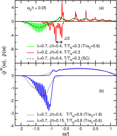
Figure 5: (color online) Spectral function $\bar{\rho}(\omega)$ and weighted spectral function $\bar{\rho}^{\rm w}(\omega)$ for the different cases reported in the legend. For better readability, the weighted spectral function $\bar{\rho}^{\rm w}(\omega)$ is reported on the negative axis. The dashed black line in panel (a) refers to the strong coupling (SC) approximate formula as discussed in Sec. V.

The evolution of the optical conductivity with $\lambda$ can be understood by analyzing the building blocks of Eqs. (11,12). In Fig. 5(a), we report both the spectral function $\bar{\rho}$ and the weighted spectral function $\bar{\rho}^{\rm w}$ for two typical values $\lambda=0.2$ and $\lambda=0.7$. In the first case (dark red curve), there is no energy separation between the single-hole excitations in $\bar{\rho}$ and the thermally excited states in $\bar{\rho}^{\rm w}$. The low-frequency gap in the optical absorption seen in Fig. 4 arises due to the explicit shift of the spectral function by the quantity $\tilde{J}/2$ in Eq. (10), representing the energy cost to create one spin-defect as the hole hops in the AF background. It is now interesting to compare these features with the results for $\lambda=0.7$ [light green curve in Fig. 5(a)]. As we can see, the spectral functions $\bar{\rho}(\omega)$ for $\lambda=0.7$ and $\lambda=0.2$ are qualitatively similar, the only major difference being the increased number of phonon satellites involved in each magnetic peak, reflecting the increased number of phonons in the polaron cloud. In order to understand the modification of the optical conductivity we thus focus on the weighted spectral function $\bar{\rho}^{\rm w}$. The latter undergoes a much more drastic change reflecting in an explicit way the signature of polaron formation. Of particular relevance is the shift of $\bar{\rho}^{\rm w}$ to much more negative energies which characterizes the lattice trapping. Note also that the magnetic peaks that are clearly visible at $\lambda=0.2$ are completely washed out at $\lambda=0.7$, merging into a broad polaronic-like spectrum centered at higher “binding” energies. This change in the nature of the thermally excited states is at the origin of both the opening of a polaronic pseudogap and of the smoothening of the features observed in $\sigma(\omega)$.

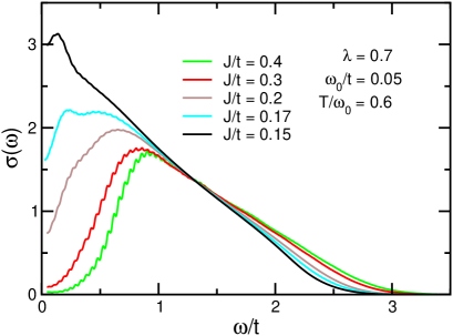
Figure 6: (color online) Optical conductivity across the polaron crossover, as varying $J$ for fixed $\lambda=0.7$, $\omega_{0}/t=0.05$ and fixed temperature $T/\omega_{0}=0.6$. Note that this fixed temperature corresponds to different $T/T_{\rm N}$ for $J/t=0.4,0.3,0.2,0.17,0.15$, respectively $T/T_{\rm N}=0.3,0.4,0.6,0.7,0.8$.

A qualitatively similar evolution is observed upon varying $J$, which gives a clear illustration of the positive interplay between magnetic and lattice polaron effects. This is shown in Fig. 6 where we report the optical conductivity for different values of $J$ at constant $\lambda=0.7$ and at the same temperature $T/\omega_{0}=0.6$ as in Fig. 4 (note that this corresponds to different $T/T_{\rm N}$ as $T_{\rm N}$ scales with $J$). Remarkably, even though $\lambda$ is kept constant, reducing the magnetic exchange from the initial value $J=0.4$ leads to a gradual loss of the lattice polaronic features and to the undressing of the hole from multi-phonon excitations. This results in a shift of spectral weight from the polaronic peak to a magnon peak at lower frequency. The magnon peak is already visible as a shoulder in the data of Fig. 6 at $J/t=0.3$ and $J/t=0.2$, and it emerges more clearly at lower values of $J$. At $J=0.17$, in particular, both the magnetic peak and the broad polaronic band are visible in the absorption spectrum. The featureless nature of the absorption curves at low $J/t$ can be ascribed to the increasing disorder of the AF environment as $J$ diminishes and $T/T_{N}$ increases.logan

Once again, the comparison of $\bar{\rho}^{\rm w}$ and $\bar{\rho}$ for $J/t=0.4$ [light green curve in 5(a)] and for $J/t=0.15$ [dark blue curve in 5(b)] allows to visualize in a simple way the loss of the polaronic features. Even in this case the most relevant quantity is the weighted spectral function $\bar{\rho}^{\rm w}$ whose main excitations, for $J=0.15$, are shifted to much less negative energies than for $J/t=0.4$, closing the gap between $\bar{\rho}^{\rm w}$ and $\bar{\rho}$. Note in addition that, although less evident than at $J/t=0.4$, a magnetic peak in the spectral function $\bar{\rho}$ is still visible even for $J/t=0.15$. The convolution of $\bar{\rho}$ with $\bar{\rho}^{\rm w}$ gives rise to the small magnetic peak at $\omega\simeq\tilde{J}/2$ observed in the optical conductivity.

In Fig. 7 we report the evolution of the optical spectra versus temperature in the polaronic regime at $\lambda=0.7$, $\omega_{0}/t=0.05$ and $J/4=0.4$. Although Fig. 7 can look at a first glance quite similar to Fig. 4, no shift of the peak of $\sigma(\omega)$ is observed here. Instead, there is a progressive filling of the low frequency gap with temperature that is quite similar to what is observed in the pure Holstein model.fratini This can be pointed out again by the comparative study of $\bar{\rho}$ with $\bar{\rho}^{\rm w}$. For $T/T_{\rm N}=0.9$ [light brown curve in 5(b)] the weighted spectral function $\bar{\rho}^{\rm w}(\omega)$ still presents an extended peak at negative energy $\omega/t\approx-1.3$, signalizing that the lattice polaron is not completely destroyed. However, the broadening of $\bar{\rho}^{\rm w}(\omega)$ is now significantly enhanced as $T\gtrsim\omega_{0}$. This feature, along with a similar broadening of the spectral function $\rho(\omega)$ due to the approaching of the paramagnetic limit $T/T_{\rm N}\rightarrow 1$ (see Sec. III), leads to a significant overlap of the two spectral functions and to a continuous filling of the gap in the optical conductivity as the temperature is increased.

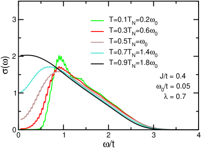
Figure 7: (color online) Temperature evolution of the optical conductivity for $\lambda=0.7$, $J/t=0.4$ and $\omega_{0}/t=0.05$.

V Strong coupling formula

In the previous section we have discussed the technical difficulties involved in the calculation of the optical conductivity. Even adopting the proposed scaling procedure (cf. Sec. IV.1), the computational cost can still be quite demanding, especially in the strong coupling lattice polaron regime where the number of phonons to be taken into account scales as $\alpha^{2}=\lambda t/\omega_{0}$. In this section we present a simple analytical formulation of the optical conductivity which is valid precisely in the adiabatic ($\omega_{0}\rightarrow 0$) small polaron regime and which involves almost no numerical effort.

The basis of this simplified formulation is the polaronic nature of the weighted spectral function $\bar{\rho}^{\rm w}$ pointed out in Fig. 5. We have seen indeed that at moderate values of the electron-lattice coupling, just above the polaron crossover, the function $\bar{\rho}^{\rm w}$ becomes essentially independent of the exchange term $J$. A closer look shows that in the lattice polaron regime the spectral function $\bar{\rho}^{\rm w}$ can be well approximated with the result of the atomic limit $t\to 0$,Mahan

$$\bar{\rho}^{\rm w}(\omega)=\frac{1}{\sqrt{2\pi s^{2}}}\exp\left[-\frac{(\omega+2\lambda t)^{2}}{2s^{2}}\right],$$ (13)

where $s=g/\sqrt{\tanh(\omega_{0}/2T)}$. This function for the case $\lambda=0.7$, $J/t=0.4$, $\omega_{0}/t=0.05$, $T/T_{\rm N}=0.3$ is shown in Fig. 5a compared with the full numerical solution for the same parameters. The good agreement can be ascribed to the atomic nature of the thermally induced excitations, which do not hybridize with the hopping continuum described by the self-energy Eq. (8) (an equivalent result was already pointed out in Ref. fratini, ). Eq. (13) provides thus a simple analytical expression for $\bar{\rho}^{\rm w}(\omega)$ which can be employed in Eq. (10) for the evaluation of the optical conductivity.

A simple analytical approximation can also be derived for the one-hole spectral function $\bar{\rho}(\omega)$ involved in Eq. (10). At this level, we are mainly interested in the overall shape of the optical conductivity $\sigma(\omega)$, disregarding the multi-phonon fine structure that will be anyway washed out at large $\lambda$ as shown in Fig. 4. In this perspective we can consider formally the limit $\omega_{0}\rightarrow 0$ and use the approach devised in Refs. polarone, ; hohu, as well as in Ref. rosch1, to treat the adiabatic limit. In particular, the sum over the discrete energy levels in Eq. (3) can be replaced by an integration over Gaussianly distributed local random energies $\nu$ which account for the thermal/quantum fluctuations of the phonon field. The local propagator thus becomespolarone ; hohu ; rosch1

$$\bar{G}(\omega)=\int d\nu\frac{P(\nu)}{{\mathcal{G}}^{-1}(\omega)-\nu},$$ (14)

where $P(\nu)=(1/\sqrt{2\pi s^{2}})\mbox{e}^{-\nu^{2}/2s^{2}}$ is a Gaussian function with the same variance as in Eq. (13 ). Self-consistency is achieved by employing Eqs. (7)-(8). The comparison between the approximate formula for $\bar{\rho}(\omega)$ valid in the polaronic regime and the full numerical solution is also shown in Fig. 5a for $\lambda=0.7$, $J/t=0.4$, $\omega_{0}/t=0.05$, $T/T_{\rm N}=0.3$. Note that, although the bath propagator ${\mathcal{G}}(\omega)$ does not depend explicitly on the local random energies $\nu$, it still depends parametrically on $\lambda$ and $J$ through the self-consistency conditions Eqs. (7)-(8), so that it still retains the relevant lattice and magnetic spectral structures.

Once the approximate analytical expressions for the spectral functions $\bar{\rho}$ and $\bar{\rho}^{\rm w}$ are provided, we can now simply evaluate the optical conductivity by using Eq. (10). Let us stress that the numerical solution of the approximate expressions for $\bar{\rho}$ and $\bar{\rho}^{\rm w}$, defined in Eqs. (13)-(14) requires a remarkably smaller computational cost than the full numerical solution, especially in the lattice polaronic regime where Eqs. (13)-(14) are valid and where the computational cost of the full numerical solution is highest. The comparison of the approximate formula with the full numerical solution as function of the electron-phonon coupling constant $\lambda$ is illustrated in Fig. 8. The agreement is excellent in the small polaron regime $\lambda\gtrsim 0.7$ and it is still quite satisfactory even for moderate electron-phonon coupling $\lambda=0.5$.

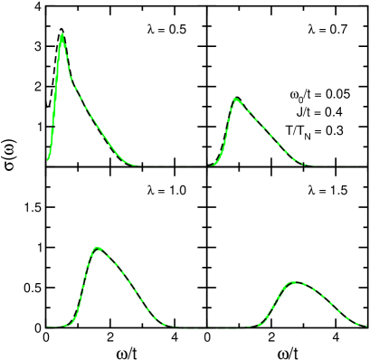
Figure 8: (color online) Comparison of the optical conductivity evaluated from the full numerical solution (light green lines) and by means of the strong coupling formula (dashed black lines). The agrement is accurate already at moderate values of $\lambda$.

VI Summary and conclusions

In this work, we have provided an analytical treatment for the optical conductivity $\sigma(\omega)$ of one hole in the Holstein-$t$-$J$ model at finite temperature, in the limit of infinite dimensions. In this context a dynamical mean-field solution can be derived where the local self-consistent problem is solved exactly. Due to intrinsic limitations enforced in infinite dimensions, we are not able to account for the coherent propagation of a single hole in the antiferromagnetic background. Nevertheless, we have shown how the incoherent optical processes, related to local excitations (Einstein phonons and local spin-flips) are well described in our approach, as confirmed by the comparison with numerical results obtained by Lanczos diagonalization.

Our main aim has been to investigate the incoherent features of $\sigma(\omega)$ in an intermediate coupling region where the positive interplay between the magnetic and lattice degrees of freedom is more relevant, sustaining the formation of a spin-lattice polaron. In this context we have studied the evolution of polaronic features in the optical conductivity as function of the different microscopic parameters, as the electron-phonon coupling $\lambda$, the temperature $T$ and the effective exchange energy $\tilde{J}$. We remind that $\tilde{J}$ does not represent the bare exchange energy but rather a mean-field-like Weiss exchange coupling which depends on the local magnetization $m$. In the cuprates, for example, this parameter can be tuned by varying the hole doping starting from the parent AF phase. We have shown that the role of the electron-phonon coupling is twofold. On one hand it rules the formation of the lattice polaron, changing the incoherent part of $\sigma(\omega)$ from a typical spin-polaron spectrum, characterized by magnetic peaks and by an optical gap at $J/2$, to a broad lattice-polaron-like shape located at higher frequency, from which the magnetic peaks are essentially washed out. On the other hand it also tunes the amount of quantum lattice fluctuations, reflected in the emergence of multi-phonon satellite peaks. This fine structure survives also when the lattice polaron is destroyed at small $\lambda$ and it gives rise to an effective broadening of the magnetic peaks which can be much larger than the intrinsic broadening driven by the thermal magnetic fluctuations.

The present approach allows us to distinguish between two different mechanisms leading to a suppression of the polaronic pseudogap: $i$) at intermediate values of the electron-phonon coupling, the reduction of the effective exchange energy $\tilde{J}$ leads to a shift of spectral weight from high energy lattice polaronic features to low energy magnetic excitations. This results in a closing of the pseudogap as the hole undresses from its lattice polaron cloud; $ii$) Conversely, increasing the temperature within the polaronic regime, gives rise to a filling of the pseudogap. Both mechanisms are actually observed in the optical spectra of the underdoped cuprates.onose

As a final remark, we briefly comment on the robustness of our results in physical systems where quantum spin fluctuations are present, allowing for coherent motion of the holes. As discussed above, one of the main effects is the emergence of a dispersive pole with small spectral weight in the one-particle spectral function. In the optical spectra, this gives rise to a Drude-like low-frequency response, but it does not affect the high-frequency incoherent part (moreover the coherent spectral weight is strongly reduced when the electron-lattice coupling is turned on). Regarding the high-frequency part, the intrinsic dispersion of the spin fluctuations is itself expected to smear the magnetic peaks. This would affect our results only in the weak electron-phonon coupling regime, where no lattice polaron is formed. In this case an intrinsic broadening of the magnetic peaks in the optical spectra due to the spin-fluctuation dispersion should be considered for a quantitative analysis. On the other hand, the effects of the dispersion of spin-fluctuations are expected to be barely visible in the lattice polaron regime, where the smearing due to the multi-phonon satellite structure around each magnetic peak dominates.

Appendix A Finite temperature Green’s function of the Holstein-$t$-$J$ model in infinite dimensions

In this Appendix we provide a detailed derivation of the Green’s function of one hole in the Holstein-$t$-$J$ model at finite temperature in the infinite dimensional limit. A formal derivation for the pure $t$-$J$ model was discussed in Ref. logan, , while the derivation for the full Holstein-$t$-$J$ model at $T=0$ was provided in Ref. cc, . On this ground, here we limit ourselves to the derivation of the finite temperature self-consistent equations in terms of continued fractions.

Let us start by writing the Hamiltonian in Eq. (1) as $H=H_{t}+H_{\rm L}$, where $H_{t}$ represents the non-local hopping term while $H_{\rm L}$ contains all the other, purely local, contributions. We also define the Green’s function as:

$$G_{i}(t) = -i\theta(t)\frac{1}{Z^{\rm T}(N)}\sum_{\{n\}_{i},\{s\}_{i}}\left\langle\{s\}_{j\neq i},\{n\}_{j\neq i};s_{i},n_{i}\right|\mbox{e}^{-\beta H}\mbox{e}^{-iHt}c_{i}^{\dagger}\mbox{e}^{iHt}c_{i}\left|n_{i},s_{i}=0;\{n\}_{j\neq i},\{s\}_{j\neq i}\right\rangle,$$ (15)

where $\left|n_{i},s_{i};\{n\}_{j\neq i},\{s\}_{j\neq i}\right\rangle$ denotes the state with $n_{i}$ phonons and $s_{i}$ spin defects ($s_{i}=0$: no spin defect, $s_{i}=1$: spin defect) on the site $i$ and with a generic set $\{n\}_{j\neq i}$ of phonons and $\{s\}_{j\neq i}$ of spin defects on all the other sites. With these notations $c_{i}=h_{i}^{\dagger}$ when $s_{i}=0$ and $c_{i}=h_{i}^{\dagger}a_{i}$ when $s_{i}=1$. In addition, $Z^{\rm T}(N)$ is the total partition function of the system in the absence of holes, $N$ being the number of sites; in this case $H_{t}$ does not contribute and $Z^{\rm T}(N)$ factorizes into a phonon and a spin part as $Z^{\rm T}(N)=Z^{\rm ph}(N)Z^{\rm spin}(N)$. Each of them can be in addition factorized with respect to the site index, e.g. $Z^{\rm spin}(N)=Z^{\rm spin}_{i}\prod_{j\neq i}Z^{\rm spin}_{j}$. Similar considerations hold true for the exponential terms $\mbox{e}^{-\beta H}\mbox{e}^{-iHt}$ which apply on the states with no holes on the right side of Eq. (15). Reminding $H_{\rm L}|n_{i},s_{i}\rangle=n_{i}\omega_{0}+s_{i}\tilde{J}/2$, we can write, after few straightforward steps, in the Fourier space:

$$G_{i}(\omega) = \sum_{n_{i},s_{i}}\frac{\mbox{e}^{-\beta[n_{i}\omega_{0}+s_{i}\tilde{J}/2]}}{Z^{\rm ph}_{i}Z^{\rm spin}_{i}}\sum_{\{n\}_{j\neq i},\{s\}_{j\neq i}}\frac{\mbox{e}^{-\beta\sum_{j\neq i}[n_{j}\omega_{0}+s_{j}\tilde{J}/2]}}{Z^{\rm ph}_{j\neq i}Z^{\rm spin}_{j\neq i}}$$ (16)

$$\times\left\langle\{s\}_{j\neq i},\{n\}_{j\neq i};s_{i},n_{i}\right|c_{i}^{\dagger}\frac{1}{\omega+n_{i}\omega_{0}+s_{i}\tilde{J}/2-H}c_{i}\left|n_{i},s_{i};\{n\}_{j\neq i},\{s\}_{j\neq i}\right\rangle.$$

This can be rewritten as

$$G_{i}(\omega) = \frac{1}{Z^{\rm ph}}\sum_{n}\mbox{e}^{-\beta n\omega_{0}}G_{i}^{nn}(\omega+n\omega_{0}),$$ (17)

where

$$G_{i}^{nn}(\omega) = \sum_{s_{i}}\frac{\mbox{e}^{-\beta s_{i}\tilde{J}/2}}{Z^{\rm spin}_{i}}\sum_{\{n\}_{j\neq i},\{s\}_{j\neq i}}\frac{\mbox{e}^{-\beta\sum_{j\neq i}[n_{j}\omega_{0}+s_{j}\tilde{J}/2]}}{Z^{\rm ph}_{j\neq i}Z^{\rm spin}_{j\neq i}}$$ (18)

$$\times\left\langle\{s\}_{j\neq i},\{n\}_{j\neq i};s_{i},n_{i}\right|c_{i}^{\dagger}\frac{1}{\omega+s_{i}\tilde{J}/2-H}c_{i}\left|n_{i},s_{i};\{n\}_{j\neq i},\{s\}_{j\neq i}\right\rangle.$$

Similarly, the factor $p_{s}=\mbox{e}^{-\beta s_{i}\tilde{J}/2}/Z^{\rm spin}_{i}$ defines the local population of spin defects which can be evaluated within the mean-field theory enforced by the infinite dimensional limit, namely $p_{1}=x$, $p_{0}=1-x$. We have thus:

$$G_{i}^{nn}(\omega)=(1-x)\bar{G}_{i,0}^{nn}(\omega)+x\bar{G}_{i,1}^{nn}(\omega),$$ (19)

with

$$\bar{G}_{i,s_{i}}^{nn}(\omega) = \sum_{\{n\}_{j\neq i},\{s\}_{j\neq i}}\frac{\mbox{e}^{-\beta\sum_{j\neq i}[n_{j}\omega_{0}+s_{j}\tilde{J}/2]}}{Z^{\rm ph}_{j\neq i}Z^{\rm spin}_{j\neq i}}\left\langle\{s\}_{j\neq i},\{n\}_{j\neq i};s_{i},n_{i}\right|c_{i}^{\dagger}\frac{1}{\omega+s_{i}\tilde{J}/2-H}c_{i}\left|n_{i},s_{i};\{n\}_{j\neq i},\{s\}_{j\neq i}\right\rangle.$$ (20)

Finally, using the definition of $c_{i}$, one can see that $\bar{G}_{i,1}^{nn}(\omega)=\bar{G}_{i,0}^{nn}(\omega+\tilde{J}/2)$, and we can write

$$G_{i}^{nn}(\omega)=(1-x)\bar{G}_{i}^{nn}(\omega)+x\bar{G}_{i}^{nn}(\omega+\tilde{J}/2),$$ (21)

where

$$\bar{G}_{i}^{nn}(\omega) = \sum_{\{n\}_{j\neq i},\{s\}_{j\neq i}}\frac{\mbox{e}^{-\beta\sum_{j\neq i}[n_{j}\omega_{0}+s_{j}\tilde{J}/2]}}{Z^{\rm ph}_{j\neq i}Z^{\rm spin}_{j\neq i}}\left\langle\{s\}_{j\neq i},\{n\}_{j\neq i};n_{i}\right|\frac{1}{\omega-H}\left|n_{i};\{n\}_{j\neq i},\{s\}_{j\neq i}\right\rangle.$$ (22)

Here $\left|n_{i};\{n\}_{j\neq i},\{s\}_{j\neq i}\right\rangle$ denotes the state with $n_{i}$ phonons on site $i$, $\{n\}_{j\neq i}$, $\{s\}_{j\neq i}$ being the phonon/spin configurations on the sites $j\neq i$ with one hole on the site $i$.

We can write Eq. (22) using the short-hand notation:

$$\bar{G}_{i}^{nn}(\omega) = \hat{P}_{i}\left\langle n_{i}\right|\frac{1}{\omega-H}\left|n_{i}\right\rangle,$$ (23)

where $|n_{i}\rangle\equiv|n_{i};\{n\}_{j\neq i},\{s\}_{j\neq i}\rangle$, and where the operator

$$\hat{P}_{i}\left\langle n_{i}\right|\ldots\left|n_{i}\right\rangle = \sum_{\{n\}_{j\neq i},\{s\}_{j\neq i}}\frac{\mbox{e}^{-\beta\sum_{j\neq i}[n_{j}\omega_{0}+s_{j}\tilde{J}/2]}}{Z^{\rm ph}_{j\neq i}Z^{\rm spin}_{j\neq i}}$$ (24)

$$\times\left\langle\{s\}_{j\neq i},\{n\}_{j\neq i}\right|\ldots\left|\{n\}_{j\neq i},\{s\}_{j\neq i}\right\rangle,$$

denotes the average over the spin and phonon configurations on all the sites but $i$. The operator $\hat{P}_{i}$ represents a direct generalization of the quantity $P(s)$ introduced by Stumpf and Logan in Ref. logan, to include the phonon degrees of freedom. It is also convenient to note that (for $j\neq i$):

$$\hat{P}_{i}\left\langle n_{i}\right|\ldots\left|n_{i}\right\rangle = \hat{P}_{i}\sum_{n_{j},s_{j}}\hat{P}_{ij}\frac{\mbox{e}^{-\beta[n_{j}\omega_{0}+s_{j}\tilde{J}/2]}}{Z^{\rm ph}_{j}Z^{\rm spin}_{j}}$$ (25)

$$\times\left\langle s_{j},n_{j},n_{i}\right|\ldots\left|n_{i},n_{j},s_{j}\right\rangle,$$

where $\hat{P}_{ij}$ is defined in similar way as $\hat{P}_{i}$ as the average over the spin and phonon configurations on all the sites except $i$ and $j$.

Having introduced the necessary definitions, from now on we can follow the derivation in Ref. cc, properly adapted to the finite temperature case. In particular we can introduce the local Green’s function $\bar{g}_{i}^{nn}(\omega)$ defined as the atomic $t=0$ limit of Eq. (23). Note that in the atomic limit $\hat{P}_{i}=1$ so that

$$\bar{g}_{i}^{nn}(\omega) = \frac{1}{\omega-n\omega_{0}}.$$ (26)

We can also generalize Eq. (23) for off-diagonal local phonon matrix elements:

$$\bar{g}_{i}^{np}(\omega) = \hat{P}_{i}\left\langle n_{i}\right|\frac{1}{\omega-H_{\rm L}}\left|p_{i}\right\rangle,$$ (27)

whose analytical expression will be provided In Eq. (32).

We can now employ the standard relation

$$\frac{1}{\omega-H} = \frac{1}{\omega-H_{\rm L}}+\frac{1}{\omega-H_{\rm L}}H_{t}\frac{1}{\omega-H_{\rm L}}$$ (28)

$$+ \frac{1}{\omega-H_{\rm L}}H_{t}\frac{1}{\omega-H_{\rm L}}H_{t}\frac{1}{\omega-H_{\rm L}}+\ldots,$$

which, on a classical spin background, gives rise to the retraceable path approximation. We have thus

$$\bar{G}_{i}^{nm}(\omega) = \bar{g}_{i}^{nm}(\omega)-\sum_{p}\bar{g}_{i}^{np}(\omega)\bar{\Sigma}_{j}^{(p)_{i}}(\omega)\bar{G}_{i}^{pm}(\omega),$$ (29)

where $\bar{\Sigma}_{j}^{(p)_{i}}(\omega)$ represents the dynamics of the hole after hopping on the neighboring site $j$. Since, in the leading term of a $1/d$ expansion, the hopping process and the further dynamics of the hole do not involve the phonon degrees of freedom on site $i$, such evolution occurs in the presence of $p$ phonons on the site $i$, which are reflected in an shift of the frequency argument, $\bar{\Sigma}_{j}^{(p)_{i}}(\omega)=\bar{\Sigma}_{j}(\omega-p\omega_{0})$. Note that $\bar{\Sigma}_{j}(\omega)$ still contains the full thermal average on the phonons at site $j$, so that it is related to the thermally averaged Green’s function defined in Eq. (17). In addition, $\bar{\Sigma}_{j}(\omega)$ will depend also on the initial spin configuration $s_{j}$ at site $j$: hopping to a site $j$ free of spin defects will create a spin defect on the site $i$, while hopping to a site $i$ with a spin defect will restore the initial magnetic background at site $i$ destroying a spin defect at $i$. Using these considerations we have thus:

$$\Sigma_{j}(\omega) = \frac{t^{2}}{4}\left[\sum_{s_{j}}p_{s_{j}}\bar{G}_{j}(\omega+(2s_{j}-1)\tilde{J}/2)\right]$$ (30)

$$=\frac{t^{2}}{4}\left[(1-x)\bar{G}_{j}(\omega-\tilde{J}/2)+x\bar{G}_{j}(\omega+\tilde{J}/2)\right],$$

and we can write Eq. (29) in the compact form:

$$\bar{G}^{nm}(\omega)=\bar{g}^{nm}(\omega)-\sum_{p}\bar{g}_{i}^{np}(\omega)\Sigma_{t}(\omega-p\omega_{0})\bar{G}^{pm}(\omega),$$ (31)

where we have dropped the unnecessary site indices and we have added the index $\Sigma_{t}$ to denote a self-energy term arising from the hopping processes.

We can indeed employ now the usual procedure to obtain the electron-phonon self-energy in terms of a continued fraction. In particular, in addition to the diagonal elements of Eq. (26), we specify also the non-diagonal ones which read:

$$\left[\bar{g}(\omega)\right]^{nm}=\left[\omega-n\omega_{0}\right]\delta_{n,m}+gX^{n,m}.$$ (32)

Using the standard derivation, we can thus write the Green’s function $\bar{G}_{i}^{nn}(\omega)$ as

$$\bar{G}^{nn}(\omega)=\frac{1}{{\cal G}^{-1}(\omega-n\omega_{0})-\Sigma_{\rm em}^{n}(\omega)-\Sigma_{\rm abs}^{n}(\omega)},$$ (33)

where ${\cal G}^{-1}(\omega)=\omega-\Sigma_{t}(\omega)$, and

$$\Sigma_{\rm em}^{n}(\omega)=\frac{(n+1)g^{2}}{\displaystyle{\cal G}^{-1}(\omega-(n+1)\omega_{0})-\frac{\displaystyle(n+2)g^{2}}{\displaystyle{\cal G}^{-1}(\omega-(n+2)\omega_{0})-\frac{\displaystyle(n+3)g^{2}}{\displaystyle\ldots}}},$$ (34)

and

$$\Sigma_{\rm abs}^{n}(\omega)=\frac{ng^{2}}{\displaystyle{\cal G}^{-1}(\omega-n\omega_{0})-\frac{\displaystyle(n-1)g^{2}}{\displaystyle{\cal G}^{-1}(\omega-(n-1)\omega_{0})-\frac{\displaystyle(n-2)g^{2}}{\displaystyle\ldots}}}.$$ (35)

Appendix B Optical conductivity

In the previous Appendix we have derived an exact expression for the Green’s function of a single hole in the Holstein-$t$-$J$ model in infinite dimensions. Here we investigate within the same framework the optical conductivity per hole, $\sigma(\omega)$, in the zero density limit. To this aim we provide an alternative derivation with respect to Ref. logan, . The main advantage of the present approach is to deal at the same level with both the spin and phonon degrees of freedom, allowing thus for an immediate generalization of the $t$-$J$ model to the Holstein-$t$-$J$ model. As a result we obtain a final expression of the optical conductivity as a functional of the one-hole Green’s function which is formally similar to the one of Ref. logan, but where the local Green’s function takes into account the electron-phonon interaction.

The formal way to derive the optical conductivity $\sigma(\omega)$ for a single charge, is to consider the limit $\sigma(\omega)=\lim_{n_{h}\rightarrow 0}\sigma(\omega;n_{h})/n_{h}$, where $\sigma(\omega;n_{h})$, $n_{h}$ are quantities defined in the grand-canonical ensemble $\langle O\rangle=\sum_{N_{h}}\mbox{e}^{\beta\mu N_{h}}\mbox{\rm Tr}\left\{O\right\}_{N_{h}}/Z_{\rm G.C.}$, and where $N_{h}$ it the total number of charges. The limit $n_{h}\rightarrow 0$ is enforced by expanding to lowest order in terms of the fugacity $z=\mbox{e}^{\beta\mu}$ ($\mu\rightarrow-\infty$). In this limit only the subsector $N_{h}=1$ survives both in $\sigma(\omega;n_{h})$ and in $n_{h}$.

Let us first consider the hole density, which we can write as:

$$n_{h}=\frac{\mbox{e}^{\beta\mu}}{Z^{\rm T}}\sum_{i,\alpha}\mbox{e}^{-\beta E_{\alpha}}\left\langle\alpha\left|h_{i}^{\dagger}h_{i}\right|\alpha\right\rangle,$$ (36)

where $|\alpha\rangle$ is a complete set of eigenstates with eigenvalues $E_{\alpha}$ of one single hole (subspace $N_{h}=1$). Here, since the state $|\alpha\rangle$ must contain one hole at site $i$, the hole-number operator is simply defined as $\hat{N}_{h,i}=h_{i}^{\dagger}h_{i}$ without any spin defect. Inserting now into Eq. (36) a complete set of eigenstates $|\gamma\rangle$ in the subspace $N_{h}=0$ (no hole) and a $\delta$-function, we obtain

$$n_{h} = \mbox{e}^{\beta\mu}\int d\omega\mbox{e}^{-\beta\omega}$$ (37)

$$\times \left[\sum_{i,\alpha,\gamma}\frac{\mbox{e}^{-\beta E_{\gamma}}}{Z^{\rm T}}\left|\left\langle\alpha\left|h_{i}^{\dagger}\right|\gamma\right\rangle\right|^{2}\delta(\omega-E_{\alpha}+E_{\gamma})\right].$$

Note that only the $|\gamma\rangle$ which do not contain any spin defect at site $i$ would contribute to Eq. (37), otherwise, after the hole $h^{\dagger}$ creation, we would end up with a state with one hole and one spin defect present, which is forbidden in the Hilbert space. We have thus:

$$n_{h} = N\mbox{e}^{\beta\mu}p_{0}\int d\omega\mbox{e}^{-\beta\omega}$$ (38)

$$\times \left[\sum_{\alpha,\gamma}\frac{\mbox{e}^{-\beta E_{\gamma}}}{Z^{\rm T}}\left|\left\langle\alpha\left|h_{i}^{\dagger}\right|\gamma\right\rangle\right|^{2}\delta(\omega-E_{\alpha}+E_{\gamma})\right],$$

where $p_{0}$ is the statistical probability to have a site with no spin defect and where now only the $|\gamma\rangle$ with no spin defect at the site $i$ are selected. The square bracket in Eq. (38) is just the local spectral function $\bar{\rho}(\omega)=-(1/\pi)\mbox{Im}\bar{G}_{0}(\omega)$, namely

$$\bar{\rho}(\omega)=\sum_{\alpha,\gamma}\frac{\mbox{e}^{-\beta E_{\gamma}}}{Z^{\rm T}}\left|\left\langle\alpha\left|h_{i}^{\dagger}\right|\gamma\right\rangle\right|^{2}\delta(\omega-E_{\alpha}+E_{\gamma}),$$ (39)

[remind that $\bar{G}_{0}(\omega)=\bar{G}(\omega)$], so that we have

$$n_{h} = N\mbox{e}^{\beta\mu}p_{0}\int d\omega\mbox{e}^{-\beta\omega}\bar{\rho}(\omega).$$ (40)

Let us turn now to the optical conductivity or, more precisely, to the current-current response function $\Pi(\omega)$ which is related to $\sigma(\omega;n_{h})$ through the relation $\sigma(\omega;n_{h})=-\mbox{Im}\Pi(\omega+i\delta)/\omega$. According to the previous argumentation, in the limit $n_{h}\rightarrow 0$ we can limit our analysis to the $N_{h}=1$ subspace and write:

$$\Pi(\tau)=-\frac{\mbox{e}^{\beta\mu}}{Z^{\rm T}}\mbox{Tr}\left\{T_{\tau}\mathcal{J}(\tau)\mathcal{J}\right\}_{N_{h}=1},$$ (41)

where $\tau$ is the imaginary time in the Matsubara space and $\mathcal{J}$ is the current operator to be defined below.

After usual manipulations we can write in the Fourier space:

$$\Pi(i\omega_{m})=\mbox{e}^{\beta\mu}\sum_{\alpha}\frac{\mbox{e}^{-\beta E_{\alpha}}}{Z^{\rm T}}\left\langle\alpha\left|\mathcal{J}\frac{1-\mbox{e}^{-\beta(H-E_{\alpha})}}{i\omega_{m}-H+E_{\alpha}}\mathcal{J}\right|\alpha\right\rangle,$$ (42)

where $\omega_{m}=2\pi mT$ are bosonic frequencies and where we remind that $|\alpha\rangle$ are eigenstates in the $N_{h}=1$ subspace.

The current density operator can be written as $\mathcal{J}=(it/2\sqrt{z})\sum_{\langle i,j\rangle}\left(c_{i}^{\dagger}c_{j}-c_{j}^{\dagger}c_{i}\right)$, where we are summing explicitly on all possible directions (this prescription compensates for the well-known vanishing of the current-current response in infinite dimensionsstrack ). As discussed in Refs. cc, ; martinez, and as appearing in Eq. (1), $c_{i}^{\dagger}c_{j}=h_{i}h_{j}^{\dagger}a_{j}$ if there is a spin defect on the site $j$ ($s_{j}=1$), while $c_{i}^{\dagger}c_{j}=a_{i}^{\dagger}h_{i}h_{j}^{\dagger}$ if there is no spin defect on the site $j$ ($s_{j}=0$). Due to the classical nature of the magnetic background, it is easy to realize that a retraceable path approximation is enforced also in the current-current response function just as in the one-particle Green’s function. We obtain thus:

$$\Pi(i\omega_{m}) = \frac{t^{2}\mbox{e}^{\beta\mu}}{4z}\sum_{\alpha}\frac{\mbox{e}^{-\beta E_{\alpha}}}{Z^{\rm T}}$$ (43)

$$\times\sum_{\langle i,j\rangle}\left\langle\alpha\left|c_{i}^{\dagger}c_{j}\frac{1-\mbox{e}^{-\beta(H-E_{\alpha})}}{i\omega_{m}-H+E_{\alpha}}c_{j}^{\dagger}c_{i}\right|\alpha\right\rangle.$$

As usual, we can now insert twice in Eq. (43) the identity operator $\sum_{\gamma}|\gamma\rangle\langle\gamma|$, where $|\gamma\rangle$ are eigenstates in the subspace without any hole. We have thus:

$$\Pi(i\omega_{m}) = \frac{t^{2}\mbox{e}^{\beta\mu}}{4z}\sum_{\alpha,\gamma,\gamma^{\prime}}\frac{\mbox{e}^{-\beta E_{\alpha}}}{Z^{\rm T}}\sum_{\langle i,j\rangle}\left\langle\alpha\left|c_{j}\right|\gamma\right\rangle\left\langle\gamma\left|c_{i}^{\dagger}\frac{1-\mbox{e}^{-\beta(H-E_{\alpha})}}{i\omega_{m}-H+E_{\alpha}}c_{i}\right|\gamma^{\prime}\right\rangle\left\langle\gamma^{\prime}\left|c_{j}^{\dagger}\right|\alpha\right\rangle.$$ (44)

Let us summarize the physical meaning of Eq. (44). The eigenstate $|\alpha\rangle$ contains one hole at the site $j$, and Eq. (44) describes the hopping of the hole to site $i$. If no spin defect is initially present at $i$ ($s_{i}=0$), this process involves the creation of a spin defect at $j$, and hence $c_{i}=h_{i}^{\dagger}$, $c_{j}^{\dagger}=a_{j}^{\dagger}h_{j}$. On the other hand, in the alternative case where a spin defect is initially present at $i$ ($s_{i}=1$), the hopping process destroys the spin defect at the site $i$, so that $c_{i}=a_{i}h_{i}^{\dagger}$ and $c_{j}^{\dagger}=h_{j}$.

Let us consider for the moment the first case. We have thus:

$$\Pi_{0}(i\omega_{m}) = \frac{t^{2}\mbox{e}^{\beta\mu}}{4z}\sum_{\alpha,\gamma,\gamma^{\prime}}\frac{\mbox{e}^{-\beta E_{\alpha}}}{Z^{\rm T}}\sum_{\langle i,j\rangle}\left\langle\alpha\left|h_{j}^{\dagger}a_{j}\right|\gamma\right\rangle\left\langle\gamma\left|h_{i}\frac{1-\mbox{e}^{-\beta(H-E_{\alpha})}}{i\omega_{m}-H+E_{\alpha}}h_{i}^{\dagger}\right|\gamma^{\prime}\right\rangle\left\langle\gamma^{\prime}\left|a_{j}^{\dagger}h_{j}\right|\alpha\right\rangle.$$ (45)

Let us now ask ourselves the following question: how much does the one-hole state $|\alpha\rangle$ differ from the “free-like” state $|\gamma\rangle$ in the absence of holes? It is clear that in the $t=0$ case only the phonon-spin configuration on the site $j$ is affected by the presence of the hole, whereas all the other sites would be unaffected. In the presence of hole dynamics ($t\neq 0$), however, all the other sites are in principle affected. We remind also that, because of the classical magnetic background, the hole dynamics obeys a retraceable path approximation just as in a Bethe lattice, as depicted in Fig. 9.

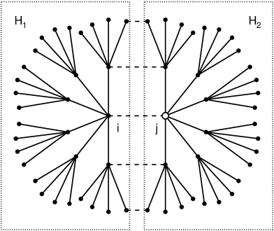
Figure 9: Schematic picture of the hole dynamics in the retraceable path approximation for $z\rightarrow\infty$. Given a hole at site $j$ [subspace (2)], the probability to affect the subspace (1), through the link $\langle i,j\rangle$ or other links (dashed connections), is $O(1/\sqrt{z})$. In the leading order $1/z\rightarrow 0$ the subspace $H_{1}$, $H_{2}$ are thus independent.

Let us consider now a given specific link of two nearest neighbor sites, $\langle i,j\rangle$. In a true Bethe lattice, the whole system can be divided in two subspaces, (1) and (2), connected by the hopping term $t_{ij}\propto t/\sqrt{z}$. This means that, to leading order, the presence of one hole on the site $j$ would not affect the subspace (1). Similar considerations hold true for a generic lattice under the retraceable path conditions: additional links between the two subspaces (dashed lines in Fig. 9), will contribute only to $O(1/\sqrt{z})$ and they can be neglected in the $z\rightarrow\infty$ limit. For practical purposes we can thus split the total Hamiltonian as $H=H_{1}+H_{2}$, where $H_{1}$ accounts for the phonon-spin degrees of freedom of the subspace (1) (not including $j$), while $H_{2}$ contains the phonon-spin degrees of freedom of the subspace (2) (not including $i$). In a similar way the eigenstates $|\alpha\rangle$, $|\gamma\rangle$ can be written (in the leading order of a $1/z$ expansion) as $|\alpha\rangle=|\alpha_{1}\rangle\otimes|\alpha_{2}\rangle$ and $|\gamma\rangle=|\gamma_{1}\rangle\otimes|\gamma_{2}\rangle$. Employing these results, and noting that $\langle\alpha|h_{j}^{\dagger}a_{j}|\gamma\rangle=\langle\alpha_{1}|h_{j}^{\dagger}a_{j}|\gamma_{1}\rangle\delta{\alpha_{2},\gamma_{2}}$, $\langle\gamma^{\prime}|a_{j}^{\dagger}h_{j}|\alpha\rangle=\langle\gamma^{\prime}_{1}|a_{j}^{\dagger}h_{j}|\alpha_{1}\rangle\delta{\gamma^{\prime}_{2},\alpha_{2}}$, $\langle\gamma|h_{i}\ldots h_{i}^{\dagger}|\gamma^{\prime}\rangle=\langle\gamma_{2}|h_{i}\ldots h_{i}^{\dagger}|\gamma^{\prime}_{2}\rangle\delta{\gamma_{1},\gamma^{\prime}_{1}}$, we have thus:

$$\Pi_{0}(i\omega_{m}) = \frac{t^{2}\mbox{e}^{\beta\mu}}{4z}\left\{\sum_{\langle j\rangle_{i},\alpha_{1},\gamma_{1}}\frac{\mbox{e}^{-\beta E_{\alpha_{1}}}}{Z^{\rm T}_{1}}\left|\left\langle\alpha_{1}\left|h_{j}^{\dagger}a_{j}\right|\gamma_{1}\right\rangle\right|^{2}\right\}$$ (46)

$$\times\left\{\sum_{i,\alpha_{2}}\frac{\mbox{e}^{-\beta E_{\alpha_{2}}}}{Z^{\rm T}_{2}}\left\langle\alpha_{2}\left|h_{i}\frac{1-\mbox{e}^{-\beta(E_{\gamma_{1}}+H_{2}-E_{\alpha_{1}}-E_{\alpha_{2}})}}{i\omega_{m}-E_{\gamma_{1}}-H_{2}+E_{\alpha_{1}}+E_{\alpha_{2}}}h_{i}^{\dagger}\right|\alpha_{2}\right\rangle\right\},$$

where $Z^{\rm T}_{1}$, $Z^{\rm T}_{2}$ are the partition functions of the corresponding subspaces and $\sum_{\langle j\rangle_{i}}$ denotes a sum over the $z$ nearest neighbors of the site $i$. Performing the analytical continuation $i\omega_{m}\rightarrow\omega+i\delta$, and introducing once more appropriate $\delta$-functions, we end up thus with:

$$\sigma_{0}(\omega;n_{h}) = -\frac{\mbox{Im}\Pi_{0}(\omega+i\delta)}{\omega}$$ (47)

$$= \frac{t^{2}\pi\mbox{e}^{\beta\mu}\left[1-\mbox{e}^{-\beta\omega}\right]}{4z\omega}\int d\Omega\mbox{e}^{-\beta\Omega}\left\{\sum_{\langle j\rangle_{i},\alpha_{1},\gamma_{1}}\frac{\mbox{e}^{-\beta E_{\gamma_{1}}}}{Z^{\rm T}_{1}}\left|\left\langle\alpha_{1}\left|h_{j}^{\dagger}a_{j}\right|\gamma_{1}\right\rangle\right|^{2}\delta(\Omega-E_{\alpha_{1}}+E_{\gamma_{1}})\right\}$$

$$\times\left\{\sum_{i,\alpha_{2},\lambda_{2}}\frac{\mbox{e}^{-\beta E_{\alpha_{2}}}}{Z^{\rm T}_{1}}\left|\left\langle\alpha_{2}\left|h_{i}\right|\lambda_{2}\right\rangle\right|^{2}\delta(\omega+\Omega-E_{\lambda_{2}}+E_{\alpha_{2}})\right\}$$

$$= \frac{t^{2}\pi N\mbox{e}^{\beta\mu}\left[1-\mbox{e}^{-\beta\omega}\right]}{4\omega}p_{0}p_{1}\int d\Omega\mbox{e}^{-\beta\Omega}\bar{\rho}_{1}(\Omega)\bar{\rho}_{0}(\omega+\Omega),$$

where $|\lambda_{2}\rangle$ are eigenstates in the $N_{h}=1$ subspace, $p_{0}=1-x$, $p_{1}=x$ are the statistical probabilities to have no spin defect and one spin defect, respectively, and where

$$\bar{\rho}_{1}(\omega)=\sum_{\alpha,\gamma}\frac{\mbox{e}^{-\beta E_{\gamma}}}{Z^{\rm T}}\left|\left\langle\alpha\left|h_{i}^{\dagger}a_{i}\right|\gamma\right\rangle\right|^{2}\delta(\omega-E_{\alpha}+E_{\gamma}).$$ (48)

The same derivation can be now employed for the case when a spin defect is present on the site $i$. After few straightforward calculations, we obtain:

$$\sigma_{1}(\omega;n_{h}) = \frac{t^{2}\pi N\mbox{e}^{\beta\mu}\left[1-\mbox{e}^{-\beta\omega}\right]}{4\omega}p_{0}p_{1}$$ (49)

$$\times\int d\Omega\mbox{e}^{-\beta\Omega}\bar{\rho}_{0}(\Omega)\bar{\rho}_{1}(\omega+\Omega).$$

Summing the two contributions (47), (49), and reminding $\bar{\rho}_{0}(\omega)=\bar{\rho}(\omega)$, $\bar{\rho}_{1}(\omega)=\bar{\rho}(\omega+\tilde{J}/2)$, after a change of variable we obtain:

$$\sigma(\omega;n_{h})=\sigma_{0}(\omega;n_{h})+\sigma_{1}(\omega;n_{h})$$ (50)

$$= \frac{t^{2}\pi N\mbox{e}^{\beta\mu}\left[1-\mbox{e}^{-\beta\omega}\right]p_{0}}{4\omega}\int d\Omega\mbox{e}^{-\beta\Omega}\bar{\rho}(\Omega)$$

$$\times\left[p_{1}\bar{\rho}(\omega+\Omega+\tilde{J}/2)+p_{0}\bar{\rho}(\omega+\Omega-\tilde{J}/2)\right],$$

where we made use also of the relation $p_{1}\mbox{e}^{\beta\tilde{J}/2}=p_{0}$. Finally, dividing Eq. (50) by (40) we obtain the dimensionless quantity Eq. (10). Note that, dividing Eq. (50) by (40), the common factors $N\mbox{e}^{\beta\mu}$ cancel out, so that the limit $\mu\rightarrow-\infty$ is well defined.

References

- (1) A.S. Mishchenko and N. Nagaosa, Phys. Rev. Lett. 93, 036402 (2004); id., Phys. Rev. B 73, 092502 (2006).
- (2) O. Rösch and O. Gunnarsson, Phys. Rev. Lett. 92, 146403 (2004); id., Eur. Phys. J. B 43, 11 (2005).
- (3) O. Rösch, O. Gunnarsson, X.J. Zhou, T. Yoshida, T. Sasagawa, A. Fujimori, Z. Hussain, Z.-X. Shen, and S. Uchida, Phys. Rev. Lett. 95, 227002 (2005).
- (4) O. Gunnarsson and O. Rösch, Phys. Rev. B 73, 174521 (2006).
- (5) P. Prelovšek, R. Zeyher, and P. Horsch, Phys. Rev. Lett. 96, 086402 (2006).
- (6) K.M. Shen, F. Ronning, D.H. Lu, W.S. Lee, N.J.C. Ingle, W. Meevasana, F. Baumberger, A. Damascelli, N.P. Armitage, L.L. Miller, Y. Kohsaka, M. Azuma, M. Takano, H. Takagi, and Z.-X. Shen, Phys. Rev. Lett. 93, 267002 (2004).
- (7) K.M. Shen, F. Ronning, W. Meevasana, D.H. Lu, N.J.C. Ingle, F. Baumberger, W.S. Lee, L.L. Miller, Y. Kohsaka, M. Azuma, M. Takano, H. Takagi, and Z.-X. Shen, Phys. Rev. B 75, 075115 (2007).
- (8) M.A. Kastner, R.J. Birgeneau, G. Shirane, and Y. Endoh, Rev. Mod. Phys. 70, 897 (1998).
- (9) D.N. Basov and T. Timusk, Rev. Mod. Phys. 77, 721 (2005).
- (10) M. Tachiki and S. Takahashi, Phys. Rev. B 38, 218 (1988).
- (11) G.A. Thomas, D.H. Rapkine, S.L. Cooper, S-W. Cheong, A.S. Cooper, L.F. Schneemeyer, and J. V. Waszczak, Phys. Rev. B 45, 2474 (1992)
- (12) A. Lucarelli, S. Lupi, M. Ortolani, P. Calvani, P. Maselli, M. Capizzi, P. Giura, H. Eisaki, N. Kikugawa, T. Fujita, M. Fujita, and K. Yamada, Phys. Rev. Lett. 90, 037002 (2003).
- (13) M. Dumm, S. Komiya, Y. Ando, and D. N. Basov, Phys. Rev. Lett. 91, 077004 (2003).
- (14) D. Mihailovic, C.M. Foster, K. Voss, and A.J. Heeger, Phys. Rev. B 42, 7989 (1990); D. Mihailovic, C.M. Foster, K.F. Voss, T. Mertelj, I. Poberaj, and N. Herron, Phys. Rev. B 44, 237 (1991).
- (15) J.P. Falck, A. Levy, M.A. Kastner, and R. J. Birgeneau, Phys. Rev. B 48, 4043 (1993).
- (16) S. Lupi, P. Maselli, M. Capizzi, P. Calvani, P. Giura and P. Roy, Phys. Rev. Lett. 83, 4852 (1999).
- (17) P. Quémerais and S. Fratini, Physica C 341, 229 (2000); S. Fratini and P. Quémerais, Eur. Phys. Journ. B 29, 41 (2002).
- (18) J. Tempere and J.T. Devreese, Phys. Rev. B 64, 104504 (2001).
- (19) T.M. Rice and F.C. Zhang, Phys. Rev. B 39, 815 (1989).
- (20) T. Timusk and D.B. Tanner, in Physical Properties of High Temperature Superconductors I, ed. by D.M. Ginsberg (World Scientific, Singapore, 1987).
- (21) For a review of early works see E. Dagotto, Rev. Mod. Phys. 66, 763 (1994). See also later papers as: J. Jaklič and P. Prelovšek, Phys. Rev. B 52, 6903 (1995); M.M. Zemljič and P. Prelovšek, Phys. Rev. B 72, 075108 (20055).
- (22) A.M. Tikofsky, R.B. Laughlin, and Z. Zou, Phys. Rev. Lett. 69, 3670 (1992).
- (23) Y. Bang and G. Kotliar, Phys. Rev. B 48, 9898 (1993).
- (24) B. Kyung and S.I. Mukhin, Phys. Rev. B 55, 3886 (1997).
- (25) G. Jackeli and N. M. Plakida, Phys. Rev. B 60, 5266 (1999).
- (26) R. Strack and D. Vollhardt, Phys. Rev. B 46, 13852 (1992).
- (27) M.P.H. Stumpf and D.E. Logan, Eur. Phys. J. B, 8, 377 (1999)
- (28) M. Jarrell, J. K. Freericks, and Th. Pruschke, Phys. Rev. B 51, 011704 (1995).
- (29) K. Haule, G. Kotliar, arXiv:cond-mat/0601478v1 (2006).
- (30) B. Baüml, G. Wellein, and H. Fehske, Phys. Rev. B 58, 3663 (1998).
- (31) B. Kyung, S.I. Mukhin, V.N. Kostur, and R.A. Ferrell, Phys. Rev. B 54, 13167 (1996).
- (32) E. Cappelluti and S. Ciuchi, Phys. Rev. B 66, 165102 (2002).
- (33) G. Sangiovanni, O. Gunnarsson, E. Koch, C. Castellani, and M. Capone Phys. Rev. Lett. 97, 046404 (2006)
- (34) S. Fratini and S. Ciuchi, Phys. Rev. B 74, 075101 (2006).
- (35) G. Martínez and P. Horsch, Phys. Rev. B 44, 317 (1991).
- (36) A. Ramšak, P. Horsch, and P. Fulde, Phys. Rev. B 46, 14305 (1992).
- (37) F. Marsiglio, A.E. Ruckenstein, S. Schmitt-Rink, and C.M. Varma, Phys. Rev. B 43, 10882 (1991).
- (38) S. Ciuchi, F. de Pasquale, S. Fratini, and D.Feinberg, Phys. Rev. B 56, 4494 (1997).
- (39) S. Fratini and S. Ciuchi, Phys. Rev. B 72, 235107 (2005).
- (40) C.L. Kane, P.A. Lee, and N. Read, Phys. Rev. B 39, 6880 (1989).
- (41) A. Khurana, Phys. Rev. Lett. 64, 1990 (1990).
- (42) We define the amplitude of the Gaussian filter as three times the variance , so that .
- (43) G.D. Mahan, Many-Particle Physics (Plenum, New York, 1981).
- (44) Y. Onose, Y. Taguchi, K. Ishizaka, and Y. Tokura, Phys. Rev. B 69, 024504 (2004).