Chemical enrichment of galaxy clusters from hydrodynamical simulations

Abstract

We present cosmological hydrodynamical simulations of galaxy clusters aimed at studying the process of metal enrichment of the intra–cluster medium (ICM). These simulations have been performed by implementing a detailed model of chemical evolution in the Tree-SPH GADGET-2 code. This model allows us to follow the metal release from SNII, SNIa and AGB stars, by properly accounting for the lifetimes of stars of different mass, as well as to change the stellar initial mass function (IMF), the lifetime function and the stellar yields. As such, our implementation of chemical evolution represents a powerful instrument to follow the cosmic history of metal production. The simulations presented here have been performed with the twofold aim of checking numerical effects, as well as the impact of changing the model of chemical evolution and the efficiency of stellar feedback. In general, we find that the distribution of metals produced by SNII are more clumpy than for product of low–mass stars, as a consequence of the different time–scales over which they are released. Using a standard Salpeter IMF produces a radial profile of Iron abundance which is in fairly good agreement with observations available out to $\simeq 0.6R_{500}$. This result holds almost independent of the numerical scheme adopted to distribute metals around star–forming regions. The mean age of enrichment of the ICM corresponds to redshift $z\sim 0.5$, which progressively increases outside the virial region. Increasing resolution, we improve the description of a diffuse high–redshift enrichment of the inter–galactic medium (IGM). This turns into a progressively more efficient enrichment of the cluster outskirts, while having a smaller impact at $R\raise-2.0pt\hbox{\hbox to0.0pt{\hbox{$\sim$}\hss}\raise 5.0pt\hbox{$<$}\ }0.5R_{500}$. As for the effect of the model of chemical evolution, we find that changing the IMF has the strongest impact. Using an IMF, which is top–heavier than the Salpeter one, provides a larger Iron abundance, possibly in excess of the observed level, also significantly increasing the [O/Fe] relative abundance. Our simulations always show an excess of low–redshift star formation and, therefore, of the abundance of Oxygen in central cluster regions, at variance with observations. This problem is not significantly ameliorated by increasing the efficiency of the stellar feedback.

1 Introduction

Observations of the power spectrum of the CMB anisotropies, combined with those of the cosmic distance scales, and the statistical properties of cosmic structures are now providing a convincing validation of the standard cosmological scenario and placing quite stringent constraints on the value of the cosmological parameters (see Springel et al., 2006, for a recent review, and references therein). As for the study of the formation process of cosmic structures, this allows us to disentangle the effects of cosmic evolution from those induced by the astrophysical processes which determine the observational properties of galaxies and of the diffuse baryons. Star formation, feedback of energy and metals from explosions of supernovae (SN) and from Active Galactic Nuclei (AGN) play a fundamental role in determining the thermo-dynamical and chemo-dynamical status of cosmic baryons.

In this respect, clusters of galaxies play a very important role. Thanks to the high density and temperature reached by the gas trapped in their potential wells, they are the ideal signposts where to trace the past history of the inter–galactic medium (IGM). Observations in the X–ray band with the Chandra and XMM–Newton satellites are providing invaluable information on the thermodynamical properties of the intra–cluster medium (ICM; see Rosati et al. 2002 and Voit 2005, for reviews). These observations highlight that non–gravitational sources of energy, such as energy feedback from SN and AGN have played an important role in determining the ICM physical properties.

At the same time, spatially resolved X–ray spectroscopy permits to measure the equivalent width of emission lines associated to transitions of heavily ionized elements and, therefore, to trace the pattern of chemical enrichment (e.g., Mushotzky, 2004, for a review). In turn, this information, as obtainable from X–ray observations, are inextricably linked to the history of formation and evolution of the galaxy population (e.g. Renzini, 1997; Pipino et al., 2002, , and references therein), as inferred from observational in the optical band. For instance, De Grandi et al. (2004) have shown that cool core clusters are characterized by a significant central enhancement of the Iron abundance in the ICM, which closely correlates with the magnitude of the Brightest Cluster Galaxies (BCGs) and the temperature of the cluster. This demonstrates that a fully coherent description of the evolution of cosmic baryons in the condensed stellar phase and in the diffuse hot phase requires properly accounting for the mechanisms of production and release of both energy and metals.

In this framework, semi–analytical models of galaxy formation provide a flexible tool to explore the space of parameters which describe a number of dynamical and astrophysical processes. In their most recent formulation, such models are coupled to dark matter (DM) cosmological simulations, to trace the merging history of the halos where galaxy formation takes place, and include a treatment of metal production from type-Ia and type-II supernovae (SNIa and SNII, hereafter; De Lucia et al. 2004; Nagashima et al. 2005; Monaco et al. 2006), so as to properly address the study of the chemical enrichment of the ICM. Cora (2006) recently applied an alternative approach, in which non–radiative SPH cluster simulations are used to trace at the same time the formation history of DM halos and the dynamics of the gas. In this approach, metals are produced by SAM galaxies and then suitably assigned to gas particles, thereby providing a chemo–dynamical description of the ICM. Domainko et al. (2006) used hydrodynamical simulations, which include simple prescriptions for gas cooling, star formation and feedback, to address the specific role played by ram–pressure stripping in determining the distribution of metals.

While these approaches offer obvious advantages with respect to standard semi–analytical models, they still do not provide a fully self–consistent picture, where chemical enrichment is the outcome of the process of star formation, associated to the cooling of the gas infalling in high density regions, as described in the numerical hydrodynamical treatment. In this sense, a fully self–consistent approach requires that the simulations must include the processes of gas cooling, star formation and evolution, along with the corresponding feedback in energy and metals.

A number of authors have presented hydrodynamical simulations for the formation of cosmic structures, which include treatments of the chemical evolution at different levels of complexity, using both Eulerian and SPH codes. Starting from the pioneering work by Theis et al. (1992), a number of chemo–dynamical models based on Eulerian codes have been presented (e.g., Samland, 1998; Recchi et al., 2001) with the aim of studying the metallicity evolution of galaxies. Although not in a cosmological framework, these analyses generally include detailed models of chemical evolution, thereby accounting for the metal production from SNIa, SNII and intermediate– and low–mass stars. Raiteri et al. (1996) presented SPH simulations of the Galaxy, forming in a isolated halo, by following Iron and Oxygen production from SNII and SNIa stars, also accounting for the effect of stellar lifetimes. Mosconi et al. (2001) presented a detailed analysis of chemo–dynamical SPH simulations, aimed at studying both numerical stability of the results and the enrichment properties of galactic objects in a cosmological context. Lia et al. (2002) discussed a statistical approach to follow metal production in SPH simulations, which have a large number of star particles, showing applications to simulations of a disc–like galaxy and of a galaxy cluster. Kawata & Gibson (2003) carried out cosmological chemo–dynamical simulations of elliptical galaxies, with an SPH code, by including the contribution from SNIa and SNII, also accounting for stellar lifetimes. Valdarnini (2003) applied the method presented by Lia et al. (2002) to an exteded set of simulated galaxy clusters. This analysis showed that profiles of the Iron abundance are steeper than the observed ones. Tornatore et al. (2004) presented results from a first implementation of a chemical evolution model in the GADGET-2 code (Springel, 2005), also including the contribution from intermediate and low mass stars. Using an earlier version of the code presented in this paper, they studied the effect of changing the prescription for the stellar initial mass function (IMF) and of the feedback efficiency on the ICM enrichment in Iron, Oxygen and Silicon. A similar analysis has been presented by Romeo et al. (2006), who also considered the effect of varying the IMF and the feedback efficiency on the enrichment pattern of the ICM. Scannapieco et al. (2005) presented another implementation of a model of chemical enrichment in the GADGET-2 code, coupled to a self–consistent model for star formation and feedback (see also Scannapieco et al., 2006). In their model, which was applied to study the enrichment of galaxies, they included the contribution from SNIa and SNII, assuming that all long–lived stars die after a fixed delay time.

In this paper we present in detail a novel implementation of chemical evolution in the Tree+SPH GADGET-2 code (Springel et al., 2001; Springel, 2005), which largely improves that originally introduced by Springel & Hernquist (2003a) (SH03 hereafter). The model by SH03 assumes that feedback in energy and metals is provided only by SNII, by assuming a Salpeter initial mass function (IMF; Salpeter, 1955), under the instantaneous recycling approximation (IRA; i.e. stars exploding at the same time of their formation). Furthermore, no detailed stellar yields are taken into account, so that the original code described a global metallicity, without following the production of individual elements. Finally, radiative losses of the gas are described by a cooling function computed at zero metallicity.

As a first step to improve with respect to this description, we properly include life-times for stars of different masses, so as to fully account for the time–delay between star formation and release of energy and metals. Furthermore, we account for the contribution of SNII, SNIa and low and intermediate mass stars to the production of metals, while only SNII and SNIa contribute to energy feedback. The contributions from different stars are consistently computed for any choice of the IMF. Also, radiative losses are computed by accounting for the dependence of the cooling function on the gas local metallicity. Accurate stellar yields are included so as to follow in detail the production of different heavy elements. The code implementation of chemical evolution is build in the GADGET-2 structure in an efficient way, so that its overhead in terms of computational cost is always very limited.

In the following of this paper, we will discuss in detail the effect that parameters related both to numerics and to the model of chemical evolution have on the pattern and history of the ICM chemical enrichment. While observational results on the ICM enrichment will be used to guide the eye, we will not perform here a detailed comparison with observations, based on a statistical ensemble of simulated clusters. In a forthcoming paper, we will compare different observational constraints on the ICM metal content with results from an extended set of simulated clusters.

The plan of the paper is as follows. In Section 2 we describe the implementation of the models of chemical evolution. After providing a description of the star formation algorithm and of its numerical implementation, we will discuss in detail the ingredients of the model of chemical evolution, finally reviewing the model of feedback through galactic winds, as implemented by SH03. In Section 3 we will present the results of our simulations. This presentation will be divided in three parts. The first one will focus on the role played by numerical effects related to the prescription adopted to distribute metals around star forming regions (Sect. 3.1). The second part will concentrate on the numerical effects related to mass and force resolution (Sect. 3.2), while the third part (Sect. 3.3) describes in detail how changing IMF, yields, feedback strength and stellar life-times affects the resulting chemical enrichment of the ICM. The readers not interested in the discussion of the numerical issues can skip Sect. 3.1 and 3.2. We will critically discuss our results and draw our main conclusions in Section 4.

2 The simulation code

We use the TreePM-SPH GADGET-2 code (Springel et al., 2001; Springel, 2005) as the starting point for our implementation of chemical evolution in cosmological hydrodynamical simulations. The GADGET-2 code contains a fully adaptive time–stepping, an explicit entropy–conserving formulation of the SPH scheme (Springel & Hernquist, 2002), heating from a uniform evolving UV background (Haardt & Madau, 1996), radiative cooling from a zero metallicity cooling function, a sub–resolution model for star formation in multi–phase interstellar medium (SH03), and a phenomenological model for feedback from galactic ejecta powered by explosions of SNII. Chemical enrichment was originally implemented by accounting only for the contribution of the SNII expected for a Salpeter IMF (Salpeter, 1955), under the instantaneous recycling approximation (IRA) using global stellar yields.

As we will describe in this Section, we have improved this simplified model along the following lines.

(a)

We include the contributions of SNIa, SNII and AGB stars to the chemical enrichment, while both SNIa and SNII contributes to thermal feedback.

(b)

We account for the age of different stellar populations, so that metals and energy are released over different time–scales by stars of different mass.

(c)

We allow for different Initial Mass Functions (IMFs), so as to check the effect of changing its shape both on the stellar populations and on the properties of the diffuse gas.

(d)

Different choices for stellar yields from SNII, SNIa and PNe are considered.

(e)

Different schemes to distribute SN ejecta around star forming regions are considered, so as to check in detail the effect of changing the numerical treatment of metal and energy spreading.

2.1 The star formation model

In the original GADGET-2 code, SH03 modeled the star formation process through an effective description of the inter-stellar medium (ISM). In this model, the ISM is described as an ambient hot gas containing cold clouds, which provide the reservoir of star formation, the two phases being in pressure equilibrium. The density of the cold and of the hot phase represents an average over small regions of the ISM, within which individual molecular clouds cannot be resolved by simulations sampling cosmological volumes.

In this description, baryons can exist in three phases: hot gas, clouds and stars. The mass fluxes between the these phases are regulated by three physical processes: (1) hot gas cools and forms cold clouds through radiative cooling; (2) stars are formed from the clouds at a rate given a Schmidt Law; (3) stars explode, thereby restoring mass and energy to the hot phase, and evaporating clouds with an efficiency, which scales with the gas density. Under the assumption that the time–scale to reach equilibrium is much shorter than other timescales, the energy from SNe also sets the equilibrium temperature of the hot gas in the star–formation regions.

The original GADGET-2 code only accounts for energy from SNII, that are supposed to promptly explode, with no delay time from the star formation episode. Therefore, the specific energy available per unit mass of stars formed is $\epsilon_{SNe}=e_{SNe}\times n_{SN}^{II}$. Here, the energy produced by a single SN explosion is assumed to be $e_{SNe}=10^{51}$ ergs, while the number of stars per solar mass ending in SNII for a Salpeter IMF (Salpeter 1955, S55 hereafter) is $n_{SN}^{II}=0.0074$ M${}_{\odot}^{-1}$.

In the effective model by SH03, a gas particle is flagged as star–forming whenever its density exceeds a given density–threshold, above which that particle is treated as multi–phase. Once the clouds evaporation efficiency and the star–formation (SF) timescale are specified, the value of the threshold is self–consistently computed by requiring (1) that the temperature of the hot phase at that density coincides with the temperature, $T_{ti}$, at which thermal instability sets on, and (2) that the specific effective energy (see eq. [11] of SH03) of the gas changes in a continuous way when crossing that threshold. Accordingly, the value of the density threshold for star formation depends on the value of the cooling function at $T_{ti}$, on the characteristic time–scale for star formation, and on the energy budget from SNII. For reference, SH03 computed this threshold to correspond to $n_{H}\simeq 0.14$ cm^-3 for the number density of hydrogen atoms in a gas of primordial composition.

In the simulations presented in this paper, we adopt the above effective model of star formation from a multi-phase medium. However, in implementing a more sophisticated model of chemical evolution we want to account explicitly for stellar life–times, thereby avoiding the approximation of instantaneous recycling, as well as including the possibility to change the IMF and the yields. Therefore, while the general structure of the SH03 effective model is left unchanged, we have substantially modified it in several aspects. Here below we describe the key features that we have implemented in the code, while we postpone further technical details to Sec. (2.3).

(1)

The amount of metals and energy produced by each star particle during the evolution are self–consistently computed for different choices of the IMF. In principle, the code also allows one to treat an IMF which changes with time and whose shape depends on the local conditions (e.g., metallicity) of the star–forming gas. This feature is not used in the simulations that we will discuss in this paper.

(2)

As in the original SH03 model, self–regulation of star formation is achieved by assuming that the energy of short–living stars is promptly available, while all the other stars die according to their lifetimes. We define as short living all the stars with mass $\geq M_{SL}$, where $M_{SL}$ must be considered as a parameter whose value ranges from the minimum mass of core–collapse SNe (we assume $8M_{\odot}$), up to the maximum mass where the IMF is computed. This allows us to parametrize the feedback strength in the self–regulation of the star formation process. We emphasize that the above mass threshold for short living stars is only relevant for the energy available to self–regulate star formation, while metal production takes place by accounting for life–times, also for stars with mass $\geq M_{SL}$. In the following runs we set $M_{SL}=8M_{\odot}$, thus assuming that all the energy from SNII is used for the self–regulation of star formation.

(3)

We include the contribution of metals to the cooling function. To this purpose, our implementation of cooling proceeds as follows. The original cooling function provided in the GADGET-2 code is used to account for the photo-ionization equilibrium of Hydrogen and Helium, while the tables by Sutherland & Dopita (1993) are used to account for the contribution of metals to the cooling function. We note that the cooling tables by Sutherland & Dopita (1993) assume the relative proportions of different metal species to be solar. Including more refined cooling rates, which depend explicitly on the individual abundances of different metal species, involves a straightforward modification of the code. Due to the lack of an explicit treatment of metal diffusion, a heavily enriched gas particle does not share its metal content with any neighbor metal poor particle. This may cause a spurious noise in the cooling process, in the sense that close particles may have heavily different cooling rates, depending on how different is their metallicity. To overcome this problem, we decided to smooth gas metallicity using the same kernel used for the computation of the hydrodynamical forces (i.e., a B–spline kernel using 64 neighbors), but only for the purpose of the computation of the cooling function. Therefore, while each particle retains its metal mass, its cooling rate is computed by accounting also for the enrichment of the surrounding gas particles.

(4)

A self–consistent computation of the density threshold for star formation implies introducing a complex interplay between different ingredients. Firstly, changing the IMF changes the amount of energy available from short–living stars, in such a way that the threshold increases with this energy. Secondly, including the dependence of the cooling function on the local metallicity causes the density threshold to decrease for more enriched star forming gas. In the following, we fix the value of this threshold at $n_{H}=0.1$ cm^-3 in terms of the number density of hydrogen atoms, a value that has been adopted in a number of previous studies of star formation in hydrodynamical simulations (e.g., Summers, 1993; Navarro & White, 1993; Katz et al., 1996; Kay et al., 2002), and which is comparable to that, $n_{H}=0.14$ cm^-3, computed by SH03 in their effective model. We defer to a future analysis the discussion of a fully self–consistent model to compute the star formation threshold.

(5)

The computation of the fraction of clouds proceeds exactly as in the original effective model (see eq.[18] in SH03), except that we explicitly include the dependence of the cooling function on the local gas metallicity, and the SN energy used for the computation of the pressure equilibrium is consistently computed for a generic IMF, as described above.

2.2 The numerical implementation of star formation

In order to the define the rule to transform star–forming gas particles into collisionless star particles we closely follow the implementation by SH03 of the algorithm originally developed by Katz et al. (1996). This algorithm describes the formation of star particles as a stochastic process, rather than as a “smooth” continuous process. Basically, at a given time the star formation rate of a multi–phase gas particle is computed using a Schmidt-type law (Schmidt, 1959):

$$\dot{m}_{\star}=xm/t_{\star}\,.$$ (1)

Here, $x$ is the fraction of gas in cold clouds, so that $xm$ is the mass of cold clouds providing the reservoir for star formation. Within the effective star formation model by SH03, the star formation time–scale, $t_{\star}({\rho})$, is computed as

$$t_{\star}(\rho)=t_{0}^{*}(\rho/\rho_{th})^{-1/2}\,,$$ (2)

where $t_{0}^{*}$ is a parameter of the model, while $\rho_{th}$ is the density threshold for star formation, that we defined above. SH03 showed that the value of $t_{0}^{*}$ should be chosen so as to reproduce the observed relation between the disc–averaged star formation per unit area and the gas surface density (Kennicutt, 1998). Following Springel & Hernquist (2003b), we assume $t_{0}^{*}=1.5$ Gyr, and checked that with this value we reproduce the Kennicutt law within the observational uncertainties.

Following eq.(1), the stellar mass expected to form in a given time interval $\Delta t$ is

$$m_{\star}=m\left\{1-\exp\left(-\frac{x\Delta t}{t_{\star}}\right)\right\}\,.$$ (3)

Within the stochastic approach to star formation, we define the number of stellar generations, $N_{*}$, as the number of star particles, which are generated by a single gas particles. Therefore, each star particle will be created with mass

$$m_{*,0}=m_{g,0}/N_{\star}\,,$$ (4)

where $m_{g,0}$ is the initial mass of the gas particles. Within this approach, a star particle is created once a random number drawn in the interval $[0,1]$ falls below the probability

$$p=\frac{m_{g,0}}{m_{*,0}}\left[1-\exp\left(-\frac{x\Delta t}{t_{\star}}\right)\right]\,.$$ (5)

After the occurrence of a large enough number of star formation events, the stochastic star formation history will converge to the continuous one. In case a gas particle already spawned $(N_{g}^{\star}-1)$ star particles, then it is entirely converted into a star particle. As we shall discuss in Section Sec. (2.3.1), star particles are allowed, in our implementation of chemical evolution, to restore part of their mass to the gas phase, as a consequence of stellar mass loss. Since this restored mass is assigned to surrounding gas particles, the latter have masses which can change during the evolution. Therefore, in the eq.(4) the actual mass $m_{g}$ replaces the initial mass $m_{g,0}$, which is assumed to be the same for all gas particles. As a consequence, star particles can have different masses due to (a) their mass loss, and (b) the mass of their parent gas particles.

Clearly, the larger the number of generations, the closer is the stochastic representation to the continuous description of star formation. In the simulations presented in this paper we will use $N_{*}=3$ as a reference value for the number of stellar generations, while we checked that there is no appreciable variation of the final results when increasing it to $N_{*}=12$.

2.3 The chemical evolution model

Due to the stochastic representation of the star formation process, each star particle must be treated as a simple stellar population (SSP), i.e. as an ensemble of coeval stars having the same initial metallicity. Every star particle carries all the physical information (e.g. birth time $t_{b}$, initial metallicity and mass), which are needed to calculate the evolution of the stellar populations, that they represent, once the lifetime function (see Section 2.3.2), the IMF (see Section 2.3.4) and the yields (see Section 2.3.3) for SNe and AGB stars have been specified. Therefore, we can compute for every star particle at any given time $t>t_{b}$ how many stars are dying as SNII and SNIa, and how many stars undergo the AGB phase, according to the equations of chemical evolution that we will discuss in Sec. (2.3.1) below. The accuracy with which chemical evolution is followed is set by defining suitable “chemical” time–steps. These time–steps are adaptively computed during the evolution by fixing the percentage of SNe of each type, which explode within each time step. In our simulations, we choose this fraction to be 10 per cent for SNII and 2 per cent for SNIa. As such, these time–steps depend both on the choice of the IMF and on the life–time function.

In the following, we assume that SNIa arises from stars belonging to binary systems, having mass in the range 0.8–8 $M_{\odot}$ (Greggio & Renzini, 1983), while SNII arise from stars with mass $>8M_{\odot}$. Besides SNe, which release energy and metals, we also account for the mass loss by the stars in the AGB phase. They contribute to metal production, but not to the energy feedback, and are identified with those stars, not turning into SNIa, in the mass range 0.8–8 $M_{\odot}$.

In summary, the main ingredients that define the model of chemical evolution, as we implemented in the code, are the following: (a) the SNe explosion rates, (b) the adopted lifetime function, (c) the adopted yields and (d) the IMF which fixes the number of stars of a given mass. We describe each of these ingredients here in the following.

As we shall discuss in Sec. (3.1), once produced by a star particle, metals are spread over surrounding particles according to a suitable kernel.

2.3.1 The equations of chemical evolution

We describe here the equations for the evolution of the rates of SNIa, SNII and AGB stars, along with their respective metal production. We provide here a short description of the basic results and of the equations, which are actually solved in our simulations, while we refer to the textbook by Matteucci (2003) for a detailed discussion.

Let $\tau(m)$ be defined as the life–time function, i.e. the age at which a star of mass $m$ dies. Accordingly, the the rate of explosions of SNIa reads

$$R_{SNIa}(t) = -\frac{\textrm{d}\,m(t)}{\textrm{d}t}\bigg{|}_{m_{2}\equiv\tau^{-1}(t)}$$

$$\times 24\,m_{2}^{2}\,A\int_{M_{Bm}}^{M_{BM}}\phi(m_{B})\frac{1}{m_{B}^{3}}dm_{B}\,.$$

where the term in the first line is the mass of stars dying at the time $t$, $\tau^{-1}(t)$ is the inverse of the lifetime function $\tau(m)$, $\phi(m)$ is the IMF and $A$ is the fraction of stars in binary systems of that particular type to be progenitors of SNIa. The integral is over the mass $m_{B}$ of the binary system, which runs in the range of the minimum and maximum allowed for the progenitor binary system, $M_{Bm}$ and $M_{BM}$, respectively. Following Greggio & Renzini (1983) and Matteucci & Greggio (1986), we assume $A=0.1$, $M_{Bm}=3M_{\odot}$ and $M_{BM}=16M_{\odot}$. Matteucci & Gibson (1995) applied a model of chemical enrichment of the ICM and found that $A=0.1$ was required to reproduce the observed Iron enrichment, by assuming a Scalo IMF (Scalo, 1986). Changing the IMF would in principle require to change the value of $A$. Since our model of ICM enrichment is quite different from that by Matteucci & Gibson (1995), we prefer here to fix the value of $A$ and check the agreement with observations for different IMFs, rather than adjusting by hand its value case by case. Eq.(2.3.1) holds under the assumption of impulsive star formation. Indeed, since each star particle is considered as a SSP, the associated star formation history, $\psi(t)$, is a delta–function, $\delta(t-t_{0})$, centered on the formation time $t_{0}$.

As for the SNII and the low and intermediate mass stars stars, the rate is given by

$$R_{SNII|AGB}(t)=\phi(m(t))\times\left(-\frac{d\,m(t)}{d\,t}\right)\,.$$ (7)

We note that the above expression must be multiplied by a factor of $(1-A)$ for AGB rates if the interested mass $m(t)$ falls in the same range of masses which is relevant for the secondary stars of SNIa binary systems.

The release of energy and chemical elements by stars (binary systems in case of SNIa) of a given mass is obtained by multiplying the above rates by the yields $p_{Z_{i}}(m,Z)$, which give the mass of the element $i$ produced by a star of mass $m$ and initial metallicity $Z$. Then, the equation which describes the evolution of the mass $\rho_{i}(t)$ for the element $i$, holding for a generic form of the star formation history $\psi(t)$, reads:

$$\begin{array}[]{l}\dot{\rho}_{i}(t)=-\psi(t)Z_{i}(t)+\\ \\ A\int_{M_{Bm}}^{M_{BM}}\phi(m)\left[\int_{\mu_{min}}^{0.5}f(\mu)\psi(t-\tau_{m_{2}})p_{Z_{i}}(m,Z)\,d\mu\right]\,dm+\\ \\ (1-A)\int_{M_{Bm}}^{M_{BM}}\psi(t-\tau(m))p_{Z_{i}}(m,Z)\varphi(m)\,dm+\\ \\ \int_{M_{L}}^{M_{Bm}}\psi(t-\tau(m))p_{Z_{i}}(m,Z)\varphi(m)\,dm+\\ \\ \int_{M_{BM}}^{M_{U}}\psi(t-\tau(m))p_{Z_{i}}(m,Z)\varphi(m)\,dm.\end{array}$$ (8)

In the above equation, $M_{L}$ and $M_{U}$ are the minimum and maximum mass of a star, respectively. In the following we use $M_{L}=0.1M_{\odot}$ and $M_{U}=100M_{\odot}$. The term in the first line of eq.(8) accounts for the metals which are locked up in stars. The term in the second line accounts for metal ejection contributed by SNIa. Here we have explicitly written the inner integral that accounts for all the possible mass ratios $\mu=m_{2}/(m_{1}+m_{2})$ between the secondary star mass and the total mass; $\mu_{\rm min}$ is the minimum value of $\mu$ and $f(\mu)$ is the corresponding distribution function. The terms on the third and fourth lines describe the enrichment by mass–loss from intermediate and low mass stars, while the last line accounts for ejecta by SNII.

The $\mu$ distribution function is assumed to be

$$f(\mu)=2^{1+\gamma}(1+\gamma)\mu^{\gamma}$$ (9)

where $\gamma=2$. This functional form of $f(\mu)$ has been derived from statistical studies of the stellar population in the solar neighborhood (Tutukov & Iungelson, 1980; Matteucci & Recchi, 2001). The value of $\mu_{\rm min}$ is calculated for a binary system of mass $M_{B}$ as

$$\mu_{\rm min}={\rm max}\left(\frac{m_{2}}{m_{B}},\frac{m_{B}-0.5M_{BM}}{m_{B}}\right).$$ (10)

Taking the impulsive star–formation, the terms in eq.(8) must be recast in the form that we actually use for calculating the rates.

In order to solve eqs.(2.3.1), (7) and (8) in the GADGET-2 code we proceed as follows. At the beginning of each run, two tables, one for SNII and one for SNIa and low and intermediate mass stars, are built to specify at what delay times the chemical evolution should be calculated. The accuracy of these “chemical time–steps” is set by two run-time parameters that specify what fraction of stars must be evolved at each step. Accordingly, during each global time-step of the code only a small fraction (typically few percent) of all stars is processed. This implementation of chemical evolution is quite efficient in terms of computational cost, especially when the number of stars grows. We verified that using $N_{*}=3$ for the number of stellar generations, the overhead associated to the chemical evolution part amounts only to $\raise-2.0pt\hbox{\hbox to0.0pt{\hbox{$\sim$}\hss}\raise 5.0pt\hbox{$<$}\ }10$ per cent of the total computational cost for a typical simulation.

2.3.2 The lifetime function

In our reference run, we use the function given by Padovani & Matteucci (1993) (PM hereafter),

$$\tau(m)=\left\{\begin{array}[]{ll}10^{[(1.34-\sqrt{1.79-0.22(7.76-\log(m))})/0.11]-9}\\ {\rm for}\,\,m\leq 6.6~{}{\rm M}_{\odot}\\ \\ 1.2\,m^{-1.85}+0.003\,\,\,\,\,{\rm otherwise}\\ \end{array}\right.$$ (11)

Furthermore, we also consider the lifetime function originally proposed by Maeder & Meynet (1989) (MM hereafter), and extrapolated by Chiappini et al. (1997) to very high ($>60M_{\odot}$) and very low ($<1.3M_{\odot}$) masses:

$$\tau(m)=\left\{\begin{array}[]{ll}10^{-0.6545\log m+1}&m\leq 1.3~{}{\rm M}_{\odot}\\ \vspace{-0.2cm}&\\ 10^{-3.7\log m+1.351}&1.3<m\leq 3~{}{\rm M}_{\odot}\\ \vspace{-0.2cm}&\\ 10^{-2.51\log m+0.77}&3<m\leq 7~{}{\rm M}_{\odot}\\ \vspace{-0.2cm}&\\ 10^{-1.78\log m+0.17}&7<m\leq 15~{}{\rm M}_{\odot}\\ \vspace{-0.2cm}&\\ 10^{-0.86\log m-0.94}&15<m\leq 53~{}{\rm M}_{\odot}\\ \vspace{-0.3cm}&\\ 1.2\times m^{-1.85}+0.003&otherwise\end{array}\right.$$ (12)

We refer to the paper by Romano et al. (2005) for a detailed discussion on the effects of different lifetime functions on the chemical enrichment model of the Milky Way.

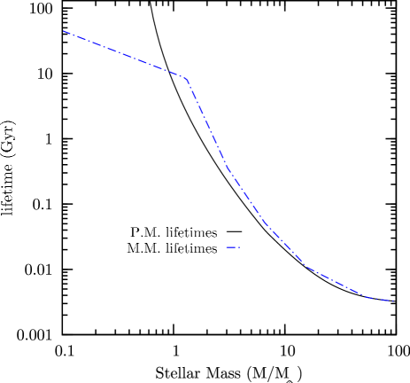
Figure 1: The dependence of the lifetime functions on the stellar mass. The solid and the dashed lines are for the lifetimes by Padovani & Matteucci (1993) and by Maeder & Meynet (1989), respectively.

A comparison between the life–time functions of eqs.(11) and (12) is shown in Figure 1. The main difference between these two functions concerns the life–time of low mass stars ($<8\,M_{\odot}$). The MM function delays the explosion of stars with mass $\raise-2.0pt\hbox{\hbox to0.0pt{\hbox{$\sim$}\hss}\raise 5.0pt\hbox{$>$}\ }1\,M_{\odot}$, while it anticipates the explosion of stars below $1\,M_{\odot}$ with respect to PM function. Only for masses below $1M_{\odot}$, the PM function predict much more long–living stars. We have verified that, assuming a Salpeter IMF (see below), the SNIa rate from a coeval stellar population is expected to be higher after $\sim 3$ Gyr when the MM lifetime function is adopted. This implies that different life–times will produce different evolution of both absolute and relative abundances. This will be discussed in more detail in Sect. 3.3.3.

We point out that the above lifetime functions are independent of metallicity, whereas in principle this dependence can be included in a model of chemical evolution. For instance, Raiteri et al. (1996) used the metallicity–dependent lifetimes as obtained from the Padova evolutionary tracks Bertelli et al. (1994).

2.3.3 Stellar yields

The stellar yields specify the quantity $p_{Z_{i}}(m,Z)$, which appears in eq.8 and, therefore, the amount of different metal species which are released during the evolution of each star particle. In the runs presented in this work, we adopt the yields provided by van den Hoek & Groenewegen (1997) the low and intermediate mass stars and by Thielemann et al. (2003) for SNIa. As for SNII we adopt the metallicity–dependent yields by Woosley & Weaver (1995) in the reference run, while we will also show the effect of using instead the yields by Chieffi & Limongi (2004) (WW and CL respectively, hereafter; see Table 2). We also assume that all the stars having masses $>40\,M_{\odot}$ directly end in black holes.

Along with freshly produced elements, stars also release non–processed elements. Sometimes, papers presenting yields table do not explicitly take into account these non–processed yields (e.g., van den Hoek & Groenewegen, 1997). In order to account for them, whenever necessary, we assume that the non–processed metals are ejected along with Helium and non–processed Hydrogen.

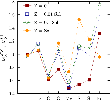
Figure 2: The ratio $M_{j}^{WW}/M_{j}^{CL}$ between the mass of species $j$, produced by the SNII of a SSP, when using the two sets of yields by Woosley & Weaver (1995) and by Chieffi & Limongi (2004) for different values of the initial SSP metallicity. Different symbols are for different values of the initial metallicity of the SSP, as reported by the labels.

Besides H and He, in the simulations presented in this paper we trace the production of Fe, O, C, Si, Mg, S. The code can be easily modified to include other metal species.

In Figure 2 we show the ratios between the abundances of different elements, as expected for the WW and the CL yields, from the SNII of a SSP. Different curves and symbols here correspond to different values of the initial metallicity of the SSP. Quite apparently, the two sets of yields provide significantly different metal masses, by an amount which can sensitively change with initial metallicity. In Sect.3.3.2 we will discuss the effect of changing yields on the resulting enrichment of the ICM and of the stellar population in simulated clusters.

2.3.4 The initial mass function

The initial mass function (IMF) is one of the most important quantity in modeling the star formation process. It directly determines the relative ratio between SNII and SNIa and, therefore, the relative abundance of $\alpha$–elements and Fe–peak elements. The shape of the IMF also determines how many long–living stars will form with respect to massive short–living stars. In turn, this ratio affects the amount of energy released by SNe and the present luminosity of galaxies, which is dominated by low mass stars, and the (metal) mass–locking in the stellar phase.

As of today, no general consensus has been reached on whether the IMF at a given time is universal or strongly dependent on the environment, or wheter it is time–dependent, i.e. whether local variations of the values of temperature, pressure and metallicity in star–forming regions affect the mass distribution of stars.

Nowadays, there are growing evidences that the IMF in the local universe, expressed in number of stars per unit logarithmic mass interval, is likely to be a power–law for $m_{\star}>1\,M_{\odot}$ with slope $x\sim 1.35$, while it becomes flat below the $1\,M_{\odot}$ threshold, possibly even taking a negative slope below $\sim 0.2\,M_{\odot}$ (e.g., Kroupa, 2001). Theoretical arguments (e.g., Larson, 1998) suggest that the present–day characteristic mass scale $\sim 1\,M_{\odot}$ should have been larger in the past, so that the IMF at higher redshift was top–heavier than at present. Chiappini et al. (2000) showed that varying the IMF by decreasing the characteristic mass with time, leads to results at variance with observations of chemical properties of the Galaxy. While the shape of the IMF is determined by the local conditions of the inter–stellar medium, direct hydrodynamical simulations of star formation in molecular clouds are only now approaching the required resolution and sophistication level to make credible predictions on the IMF (e.g., Bate & Bonnell, 2005).

In order to explore how the IMF changes the pattern of metal enrichment, we implement it in the code in a very general way, so that we can easily use both single-slope and multi–slope IMFs, as well as time–evolving IMFs. In this work we use single-slope IMFs defined as

$$\phi(m)\,=\,\textrm{d}\,{N}/\textrm{d}{\log m}\propto m^{-x}$$ (13)

using $x=1.35$ for the standard Salpeter IMF (Salpeter, 1955) in our reference run. In the above equation, $N$ is the number of stars per unit logarithmic mass interval. We will explore the effect of changing the IMF by also using a top–heavier IMF with $x=0.95$ (Arimoto & Yoshii, 1987, AY hereafter), as well as the multi–slope IMF by Kroupa (2001), which is defined as

$$\phi(m)\,\propto\,\left\{\begin{array}[]{ll}m^{-1.7}&m\geq 1\,{\rm M}_{\odot}\\ \vspace{-0.2cm}&\\ m^{-1.2}&0.5\leq m<1\,{\rm M}_{\odot}\\ \vspace{-0.2cm}&\\ m^{-0.3}&m\leq 0.5\,{\rm M}_{\odot}\\ \end{array}\right.$$ (14)

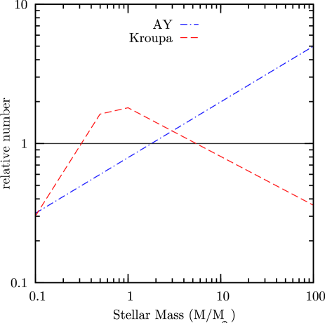
Figure 3: The dependence of the shape of the IMF on the stellar mass, relative to the Salpeter IMF (Salpeter, 1955). Dashed and dot-dashed curves are for the IMF by Arimoto & Yoshii (1987) and by Kroupa (2001), respectively. The horizontal solid line indicates for reference the Salpeter IMF.

We show in Figure 3 the number of stars, as a function of their mass, predicted by the AY and Kroupa IMFs, relative to those predicted by the Salpeter IMF. As expected, the AY IMF predicts a larger number of high–mass stars and, correspondingly, a smaller number of low–mass stars, the crossover taking place at $\simeq 2M_{\odot}$. As a result, we expect that the enrichment pattern of the AY IMF will be characterized by a higher abundance of those elements, like Oxygen, which are mostly produced by SNII. On the other hand, the Kroupa IMF is characterized by a relative deficit of high–mass stars and, correspondingly, a relatively lower enrichment in Oxygen is expected.

Since clusters of galaxies basically behave like “closed boxes”, the overall level of enrichment and the relative abundances should directly reflect the condition of star formation. While a number of studies have been performed so far to infer the IMF shape from the enrichment pattern of the ICM, no general consensus has been reached. For instance, Renzini (1997), Pipino et al. (2002) and Renzini (2004) argued that both the global level of ICM enrichment and the $\alpha$/Fe relative abundance can be reproduced by assuming a Salpeter IMF, as long as this relative abundance is subsolar. Indeed, a different conclusion has been reached by other authors (e.g., Loewenstein & Mushotzky, 1996) in the attempt of explaining $[\alpha/{\rm Fe}]>0$ in the ICM. For instance, Portinari et al. (2004) used a phenomenological model to argue that a standard Salpeter IMF can not account for the observed $\alpha$/Fe ratio in the ICM. A similar conclusion was also reached by Nagashima et al. (2005), who used semi–analytical models of galaxy formation to trace the production of heavy elements, and by Romeo et al. (2006), who used hydrodynamical simulations including chemical enrichment. Saro et al. (2006) analysed the galaxy population from simulations similar to those presented here. This analysis led us to conclude that runs with a Salpeter IMF produce a color–magnitude relation that, with the exception of the BCGs, is in reasonable agreement with observations. On the contrary, the stronger enrichment provided by a top–heavier IMF turns into too red galaxy colors.

In summary, our implementation of chemical evolution is quite similar to that adopted by Kawata & Gibson (2003) and by Kobayashi (2004), while differences exist with respect to other implementations. For instance, Raiteri et al. (1996) and Valdarnini (2003) also used a scheme similar to ours, but neglected the contribution from low- and intermediate-mass stars. Lia et al. (2002) adopted a coarse stochastic description of the ejecta from star particles: differently from our continuous description, in which enriched gas is continuously released by star particles, they assumed that each star particle is assigned a given probability to be entirely converted into an enriched gas particle. Finally, Mosconi et al. (2001) and Scannapieco et al. (2005) neglected delay times for SNII, assumed a fixed delay time for SNIa and neglected the contribution to enrichment from low- and intermediate-mass stars.

2.4 Feedback through galactic winds

SH03 discussed the need to introduce an efficient mechanism to thermalize the SNe energy feedback, in order to regulate star formation, thereby preventing overcooling. To this purpose, they introduced a phenomenological description for galactic winds, which are triggered by the SNII energy release. We provide here a basic description of this scheme for galactic winds, while we refer to the SH03 paper for a more detailed description. The momentum and the kinetic energy carried by these winds are regulated by two parameters. The first one specifies the wind mass loading according to the relation, $\dot{M}_{W}=\eta\dot{M}_{*}$, where $\dot{M}_{*}$ is the star formation rate. Following SH03, we assume in the following $\eta=3$. The second parameter determines the fraction of SNe energy that powers the winds, ${1\over 2}\dot{M}_{W}v_{W}^{2}=\chi\epsilon_{SNe}\dot{M}_{*}$, where $\epsilon_{SNe}$ is the energy feedback provided by the SNe under the IRA for each $M_{\odot}$ of stars formed. In the framework of the SH03 effective model for star formation, winds are uploaded with gas particles which are stochastically selected among the multiphase particles, with a probability proportional to their local star formation rate. As such, these particles come from star–forming regions and, therefore, are heavely metal enriched. Furthermore, SH03 treated SPH particles that become part of the wind as temporarily decoupled from hydrodynamical interactions, in order to allow the wind particles to leave the dense interstellar medium without disrupting it. This decoupling is regulated by two parameters. The first parameter, $\rho_{\rm dec}$, defines the minimum density the wind particles can reach before being coupled again. Following SH03, we assumed this density to be 0.5 times the threshold gas density for the onset of star formation. The second parameter, $l_{\rm dec}$, provides the maximum length that a wind particle can travel freely before becoming hydrodynamically coupled again. If this time has elapsed, the particle is coupled again, even if it has not yet reached $\rho_{\rm dec}$. We assumed $l_{\rm dec}=10\,h^{-1}$kpc.

While we leave the scheme of kinetic feedback associated to wind galactic unchanged, we decide to use instead the value of the wind velocity, $v_{w}$, as a parameter to be fixed. For the reference run, we assume $v_{w}=500\,{\rm km\,s^{-1}}$. With the above choice for the wind mass loading and assuming that each SN provides an energy of $10^{51}$ ergs, this value of $v_{w}$ corresponds to $\epsilon_{SNe}\simeq 1$ for a Salpeter IMF. We will also explore which is the effect of assuming instead a stronger feedback, with $v_{w}=1000\,{\rm km\,s^{-1}}$, on the pattern of chemical enrichment.

3 Results

In this Section we will discuss the results of a set of simulations of one single cluster. The cluster that we have simulated has been extracted from a low–resolution cosmological box for a flat $\Lambda$CDM cosmology with $\Omega_{m}=0.3$ for the matter density parameter, $h=0.7$ for the Hubble parameter, $\Omega_{b}=0.039$ for the baryon density parameter and $\sigma_{8}=0.8$ for the normalization of the power spectrum of density perturbations. Using the Zoomed Initial Condition (ZIC) technique (Tormen et al., 1997), mass resolution is increased in the Lagrangian region surrounding the cluster, while also high–frequency modes of the primordial perturbation spectrum are added. The main characteristics of this cluster (Cl1 hereafter) are summarized in Table 1, along with the mass resolution and the Plummer–equivalent softening parameter used in the runs (note that the softenings are set fixed in physical units from $z=2$ to $z=0$, while they are fixed in comoving units at higher redshift).

The reference run of Cl1 is performed under the following assumptions: (a) metals produced by a star particle are distributed to surrounding gas particles by using a SPH spline kernel with density weighting over 64 neighbors for the distribution of metals around star forming particles (see Sect. 3.1); (b) Salpeter IMF; (c) stellar yields from Thielemann et al. (2003) for SNIa, van den Hoek & Groenewegen (1997) for the low and intermediate mass stars and Woosley & Weaver (1995) for SNII; (d) Life–time function from Padovani & Matteucci (1993); (e) $v_{w}=500\,{\rm km\,s^{-1}}$ for the velocity of winds. In the following we will show the effect of changing each one of these assumptions. Therefore, we will explore neither the cluster-by-cluster variation in the enrichment pattern of the ICM, nor any dependence on the cluster mass. We perform instead a detailed study of the effect of changing a number of parameters which specify both the numerical details of the implementation of the model of chemical evolution model. We defer to a forthcoming paper the properties of the ICM enrichment for a statistical ensemble of simulated galaxy clusters. We summarize in Table 2 the aspects in which the various runs of Cl1 differ from the reference one.

In addition, we also performed simulations of another cluster (Cl2 in Table 1), whose initial conditions are generated at three different resolutions, for the same cosmological model, by spanning a factor 15 in mass resolution (see also Borgani et al. 2006). The lowest resolution at which the Cl2 cluster is simulated is comparable to that of the Cl1 runs. As such, this series of runs, that is performed for the same setting of the Cl1 reference (R) run, allows us to check in detail the effect of resolution on the ICM chemical enrichment.

Besides global properties, we will describe the details of the ICM enrichment by showing radial profiles of the Iron abundance and of the relative abundances of [O/Fe] and [Si/Fe], the histograms of the fraction of gas and stars having a given level of enrichment, and the time evolution of the metal production and enrichment. A comparison with observational data will only be performed for the abundance profiles of Iron, which is the element whose distribution in the ICM is best mapped. As a term of comparison, we will use a subset of 5 clusters, out of the 16, observed with Chandra and analysed by Vikhlinin et al. (2005). These clusters are those having temperature in the range 2–4 keV, comparable to that of the simulated Cl1 and Cl2 clusters. Since the profiles of Fe abundance are compared with observations, we plot them out to $R_{500}$ which is the maximum scale sampled by observations. We plot instead profiles of [Si/Fe] and [O/Fe] out to 2$R_{\mathrm{vir}}$in order to show the pattern of relative enrichment over a large enough range of scales, where the different star formation histories generates different contributions from stars of different mass. Here and in the following we assume that a SPH particle belongs to the hot diffuse gas of the ICM when it meets the following three conditions: (i) whenever the particle is tagged as multiphase, its hot component should include at least 90 per cent of its mass; (ii) temperature and density must not be at the same time below $3\times 10^{4}$K and above $500\bar{\rho}_{bar}$ respectively, where $\bar{\rho}_{bar}$ is the mean cosmic baryon density. While observational data on the Iron abundance profiles are used to “guide the eye”, we emphasize that the primary aim of this paper is not that of a detailed comparison with observations. This would require a statistically significant set of simulated clusters, sampling a wider range of temperatures, and is deferred to a forthcoming paper.

Cluster $M_{\rm 200}$ $R_{\rm 200}$ $m_{gas}$ $\epsilon_{Pl}$ $10^{14}\,h^{-1}M_{\odot}$ $\,h^{-1}{\rm Mpc}$ $10^{8}\,h^{-1}M_{\odot}$ $h^{-1}$kpc Cl1 2.2 0.98 5.7 5.0 Cl2 1.4 0.85 R1 2.31 5.2 R2 0.69 3.5 R3 0.15 2.1

Table 1: Basic properties of the two simulated clusters Column 1: cluster name; Column 2: mass within the radius, $R_{200}$, encompassing an overdensity of 200 times the critical density, $\rho_{c}$; Column 3: value of $R_{200}$; Column 4: initial mass of the gas particles; Column 5: Plummer–equivalent softening of the gravitational force at $z=0$.

R	Reference run
N16/N128	B-spline kernel for metal distribution with 16/128 neighbors
MW	B-spline kernel for metal distribution using mass weighting
TH	Top–hat kernel for metal distribution
AY	Top–heavier IMF (Arimoto & Yoshii 1987)
Kr	Kroupa IMF (Kroupa, 2001)
CL	Yields for SNII from Chieffi & Limongi (2004)
NW	No feedback associated to winds
SW	Strong winds with $v_{w}=1000\,{\rm km\,s^{-1}}$
MM	Life–time function by Maeder & Meynet (1989)

Table 2: Characteristics of the different Cl1 runs with respect to the reference run (see text). Column 1: Name of the run; Column 2: characteristic of the run.

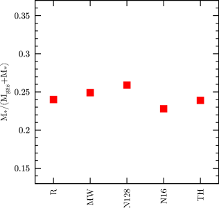
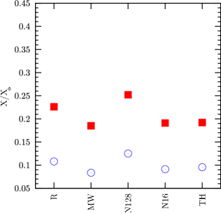
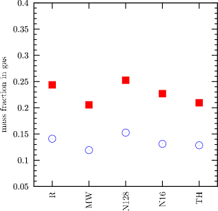
Figure 4: The effect of the numerical parameters, which define the distribution of metals, on global quantities computed within the virial radius of the Cl1 cluster: total mass fraction of baryons in stars (left panel), mass–weighted Iron abundance (central panel) and fraction of metal mass in the diffuse gas (right panel). In the central and in the right panels, filled squares refer to Iron while open circles refer to Oxygen. The labels indicating the different runs are as reported in Table 2.

3.1 The effect of metal spreading

A crucial issue in the numerical modeling of ICM enrichment concerns how metals are distributed around the star particles, where they are produced. In principle, the diffusion of metals around star forming regions should be fully determined by local physical processes, such as thermal motions of ions (e.g., Sarazin, 1988), turbulence (Rebusco et al., 2005), ram–pressure stripping (e.g., Domainko et al., 2006), galactic ejecta (e.g., Strickland & Heckman, 2006). However, for these mechanisms to be correctly operating in simulations, it requires having high enough resolution for them to be reliably described. A typical example is represented by turbulent gas motions (e.g., Rebusco et al., 2005). The description of turbulence requires not only sampling a wide enough dynamical range, where the energy cascade takes place, but also a good knowledge of the plasma viscosity, which determine the scale at which turbulent energy is dissipated (e.g., Dolag et al., 2005). While approaches to include physical viscosity in the SPH scheme have been recently pursued (Sijacki & Springel, 2006b), a full accounting for its effect requires including a self–consistent description of the magnetic field which suppresses the mean free path of ions.

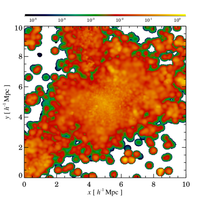
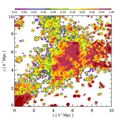
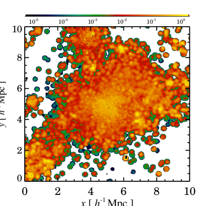
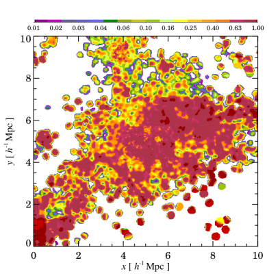
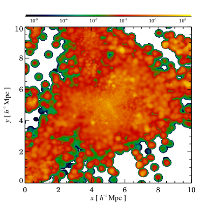
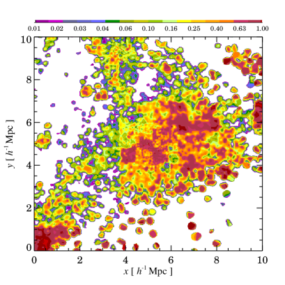
Figure 5: Maps of gas metallicity for the three different IMFs. Top, central and bottom panels refer to the Salpeter (1955) IMF, to the top–heavy (Arimoto & Yoshii, 1987) IMF and to the Kroupa (2001) IMF, respectively. The left panels are for the Iron abundance, while the right panels show the fractional contribution of SNII to the global metallicity. For reference, the virial region of the cluster is marked with the white square. The maps have been done by smoothing the contribution of each gas particle with a SPH kernel using the corresponding smoothing length. The projection has been done through a slice of $1\,h^{-1}{\rm Mpc}$ thickness, around the centre of the cluster.

Owing to the present limitations in a fully self–consistent numerical description of such processes, we prefer to adopt here a simplified numerical scheme to describe the diffusion of metals away from star forming regions. We will then discuss the effect of modifying this scheme, so as to judge the robustness of the results against the uncertainties in the modeling of the metal transport and diffusion.

Every time a star particle evolves, the stars of its population, the ejected heavy elements and energy must be distributed over the surrounding gas. The code accomplishes this task by searching for a number $N_{g}$ of gas neighbours and then using a kernel to spread metals and energy according to the relative weights that the kernel evaluation assigns to each gas particle. In this way, the fraction of metals assigned to the $i$–th neighbour gas particle can be written as

$$w_{i}\,=\,\frac{W_{i}}{\sum_{j=1}^{N_{nb}}W_{j}}\,.$$ (15)

where $W_{i}$ is kernel value at the position of the $i$-th particle $N_{nb}$ is the number of neighbors over which metals are distributed and the denominator enforce conservation of the mass in metals.

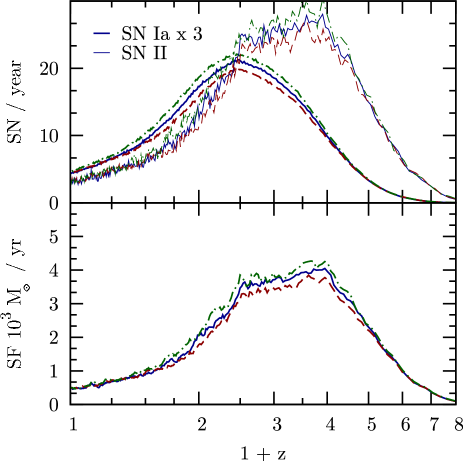
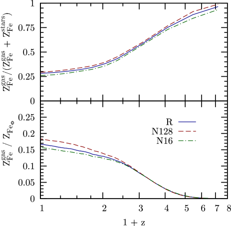
Figure 6: Left panel: the effect of changing the number of neighbours for metal spreading on the star formation rate (bottom) and on the SN rates (top; heavy and solid lines are for SNIa and SNII, respectively). Right panel: the enrichment history of Iron. The bottom panel shows the evolution of the mean Iron abundance in the gas; the top panel is for the evolution of the fraction of the total mass of Iron which is in the diffuse gas, the rest being locked in stars. In all panels, solid, dashed and dot-dashed curves are for the reference run (R), for the runs using 128 (N128) and 16 (N16) neighbors for metal spreading, respectively, when using the B-spline kernel with density weighting.

As for the weighting function $W$, the most natural choice, which is the one usually adopted in the SPH chemo–dynamical models so far presented in the literature, is to use the same B-spline kernel used for the computation of the hydrodynamical quantities, also using the same number of neighbors (e.g., Mosconi et al., 2001). Since it is a peaked function that rapidly declines to zero, it seems suitable to mimic what would be the expected behaviour of the metal deposition process. Nevertheless, it may be argued that the stochastic nature of the star formation algorithm, that samples the underlying “real” star formation on a discrete volume, should require weighting equally all the volume surrounding each stars particle. In order to judge the sensitivity of the resulting enrichment pattern on the choice of the weighting kernel, we will discuss in the following the effects of using instead a top–hat filter.

Once the functional form of $W$ is defined, one should choose the physical quantity with respect to which the weight is assigned. A first possibility is to weight according to the mass $m_{g}$ of each gas particle, in such a way that more massive particles receive a relatively larger amount of metals. An alternative choice is to weight instead according to the SPH volume carried by each particle, i.e. using the quantity $m_{g}/\rho_{g}$, where $\rho_{g}$ is the gas density associated to a particle. With this choice one gives more weight to those particles which sample a larger volume and, therefore, collect a larger amount of metals, under the assumption that they are released in a isotropic way by each star particle. Therefore, one expects that weighting according to the volume assigns more metals to gas particles which are relatively more distant from the star forming regions and, therefore, at lower density.

In the following, we will assume in our reference run that the spreading of metals is performed with the spline kernel, by weighting over 64 neighbors according to the volume of each particle. In order to check the stability of the results, we also modified the scheme for metal and energy spreading in the following ways: (i) use the same kernel and density weighting, but with 16 and 128 neighbours (N16 and N128 runs, respectively); (ii) weight according to the mass of the gas particle, instead of according to its volume, using $N_{nb}=64$ (MW run); (iii) use a top–hat window encompassing 64 neighbors, weighting by mass (TH run).

Figure 4 shows the global properties of the simulated cluster at $z=0$, in terms of amount of stars produced, mass–weighted ICM metallicity and fraction of metals in the gas, for the different numerical schemes used to distribute metals. In general, we note that changing the details of the metal spreading has only a modest effect on the overall stellar population and level of enrichment. We find that the amount of stars within the cluster virial region ranges between 23 and 26 per cent of the total baryon budget. As for the global ICM enrichment, it is $Z_{Fe}\simeq(0.20-0.25)Z_{Fe,\odot}$ and $Z_{O}\simeq 0.15Z_{O,\odot}$ for the mass–weighted Iron and Oxygen abundance, respectively. Quite interestingly, only about a quarter of the total produced Iron is in the diffuse hot gas, while this fraction decreases to about 15 per cent for Oxygen. This different behaviour of Oxygen and Iron can be explained on the ground of the different life–times of the stars which provide the dominant contribution to the production of these elements. Since Oxygen is produced by short–living stars, it is generally released in star forming regions and therefore likely to be distributed among star–forming gas particles. For this reason, Oxygen has a larger probability to be promptly locked back into stars. On the other hand, Iron is largely contributed by long–living stars. Therefore, by the time it is released, the condition of star formation around the parent star particle may be significantly changed. This may happen both as a consequence of the suppression of star formation inside galaxies or because the star particle may have later taken part to the diffuse stellar component (e.g., Murante et al., 2004). In both cases, Iron is more likely to be distributed among non star–forming particles and, therefore, contributes to the ICM enrichment, instead of being locked back in stars.

This effect is clearly visible in the right panels of Figure 5, where we show the map of the fractional contribution of SNII to the global metal enrichment. Clearly, SNII provide a major contribution (magenta–red color) in high–density patchy regions, within and around the star forming sites. On the contrary, the contribution from SNIa and AGB dominates in the diffuse medium. This is a typical example of how the pattern of the ICM enrichment is determined by the competing effects of the chemical evolution model and of the complex dynamics taking place in the dense environment of galaxy clusters. It confirms that a detailed study of the chemical enrichment of the diffuse gas indeed requires a correct accounting of such dynamical effects. We find that the contribution in Oxygen within the cluster virial radius from SNII, from SNIa and from low– and intermediate mass stars is of about 70, 5 and 25 per cent respectively, while that in Iron is 25, 70 and 5 per cent. This demonstrates that none of these three sources of metals can be neglected in a detailed modelling of the chemical enrichment of the ICM. As shown in the left panels of Fig. 5, the distribution of Iron generally follows the global large–scale structure of gas inside and around the cluster, with an excess of enrichment inside the virial region and along the filaments from which the cluster accrete pre–enriched gas. We will comment in Sect. 3.3.1 the dependence of this enrichment pattern on the IMF.

Quite interestingly, Gal-Yam et al. (2003) discovered two SNIa not associated to cluster galaxies in Virgo and argued that up to about 30 per cent of the SNIa parent stellar population is intergalactic (see also Maoz et al., 2005). This is exactly the SNIa population that in our simulations is responsible for the diffuse enrichment in Iron. As the statistics of the observed population of intergalactic SNIa population improves, it will be interesting to compare it with the predictions of our simulations and to better quantify their contribution to the ICM enrichment.

Figure 6 shows how the history of enrichment and of star formation changes by changing the scheme for distributing metals. In the left panel, the star–formation rate (SFR) is compared to the rate of SN explosions. As expected, the SNII rate follows quite closely the SFR (see left panel), and peaks at $z\simeq 2$–3. On the other hand, the rate of SNIa is substantially delayed, since they arise from stars with longer life–times. Therefore, this rate peaks at $z\simeq 1.5$ with a slower decline at low redshift than for SNII. Since the rate of SNIa is given by the combined action of SFR, life–time function and IMF, computing it by adding a constant time–delay to the SFR is generally too crude and inaccurate an approximation. As shown in Figure 7, the different redshift dependence of the SNIa and SNII rates is reflected by the different histories of enrichment in Iron and Oxygen. Since Oxygen is only contributed by short–living stars, the corresponding gas enrichment stops at $z\raise-2.0pt\hbox{\hbox to0.0pt{\hbox{$\sim$}\hss}\raise 5.0pt\hbox{$<$}\ }1$, when the SFR also declines. On the contrary, the gas enrichment in Iron keeps increasing until $z=0$, as a consequence of the significant SNIa rate at low redshift. An interesting implication of Fig.7 is that the relative abundance of Oxygen and Iron in the ICM can be different from that implied by the stellar yields. Therefore, the commonly adopted procedure to compare X–ray measurements of relative ICM abundances to stellar yields (e.g., Finoguenov & Ponman, 1999; Baumgartner et al., 2005) may lead to biased estimates of the relative contributions from SNIa and SNII (e.g., 2005PASA...22..49). We finally note that observations of SNIa rates in clusters indicates fairly low rates, for both nearby and distant objects (e.g., Gal-Yam et al., 2002), also consistent with the rates observed in the field. We postpone to a future analysis a detailed comparison between the observed and the simulated SNIa rates, and the implications on the parameters defining the model of chemical enrichment.

Figure 7: The evolution of enrichment for the reference (R) run in both Iron (solid curves) and Oxygen (dashed curves). The bottom panel shows the evolution of the mean abundances in the gas, while the top panel is for the evolution of the fraction of the total metal mass which is in the diffuse gas, the rest being locked in stars.

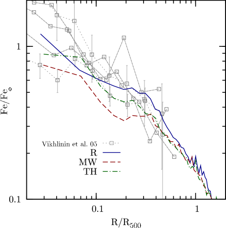
Figure 8: The effect of changing the metal spreading on the Iron abundance profiles. Left panel: comparison between the reference run (solid curve) and runs done by changing the number of neighbours to 16 (N16; short–dashed line) and to 128 (N128; long–dashed line). Right panel: comparison between the reference run (solid curve) and the runs in which metal spreading is performed using mass–weighting with the SPH kernel (MW; short–dashed line) and the top–hat kernel (TH; long–dashed line). The data points refer to a subset of four clusters, out of 16 observed with Chandra ana analysed by Vikhlinin et al. (2005), which have temperature in the range 2–4 keV. For reasons of clarity, errorbars are not reported.

In general, using a different number of neighbours to spread metals has only a minor impact on the history of star formation and enrichment (see Fig. 6). We only note that increasing the number of neighbors turns into a slight increase of the SFR at all redshifts, with a corresponding slight increase of the metallicity. In fact, increasing the number of neighbours has the effect of distributing metals more uniformly among gas particles. This causes a larger number of particles to have a more efficient cooling and, therefore, to become eligible for star formation.

In the left panel of Figure 8 we show the effect of changing the number of neighbors over which to distribute metals on the profile of the Iron abundance. As expected, increasing the number of neighbors corresponds to an increasing efficiency in distributing metals outside star forming regions. As a result, metallicity profiles becomes progressively shallower, with a decrease in the central regions and an increase in the outer regions. Although this effect is not large, it confirms the relevance of understanding the details of the mechanisms which determine the transport and diffusion of the metals.

As for the comparison with data, we note that the differences between the different weighting schemes are generally smaller than the cluster-by-cluster variations of the observed abundance gradients. In general, the simulated profiles are in reasonable agreement with the observed ones. A more detailed comparison with observed abundance profiles will be performed in a forthcoming paper, based on a larger set of simulated clusters (Fabjan et al. in preparation).

Finally, we show in the right panel of Figure 8 the variation of the Iron abundance profile when changing the weighting scheme for the distribution of metals, while keeping fixed to 64 the number of neighbors. As for the Iron profile, using volume, instead of mass, in the SPH kernel has a rather small effect. Only in the innermost bin, the Iron abundance increases when weighting according to the mass as a result of the less effective spreading to less dense gas particles. As for the top–hat kernel, its Iron profile lies below the other ones at all radii, although by a rather small amount.

3.2 The effect of resolution

In this Section we present the results of the simulations of the Cl2 cluster, done at three different resolutions (see Table 1).

Figure 10 shows the effect of resolution on the rates of star formation and SN explosions (left panel) and on the history of chemical enrichment (right panel). As expected, increasing resolution enhances the high–redshift tail of star formation, as a consequence of the larger number of resolved small halos which collapse first and within which gas cooling occurs efficiently. Quite interestingly, the increase with resolution of the high–$z$ star formation rate is compensated by a corresponding decrease at lower, $z\raise-2.0pt\hbox{\hbox to0.0pt{\hbox{$\sim$}\hss}\raise 5.0pt\hbox{$<$}\ }1$, redshift. As a net result, the total amount of stars formed within the cluster virial region by $z=0$ (left panel of Figure 9) turns out to be almost independent of resolution. This results is in line with that already presented by Borgani et al. (2006) for a similar set of simulations, but not including the chemical enrichment. On the one hand, increasing resolution increase the cooling consumption of gas at high redshift, thereby leaving a smaller amount of gas for subsequent low–$z$ star formation. On the other hand, smaller halos, forming at higher redshift when increasing resolution, generate winds which can more easily escape the shallow potential wells. As a result, the gas is pre–heated more efficiently, so as to reduce the later star formation.

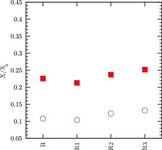
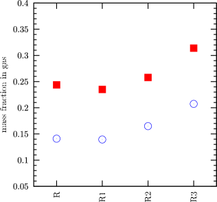
Figure 9: The same as in Figure 4, but for the runs of the Cl2 cluster at three different resolutions. The labels indicating the different runs are as reported in Table 2.

In spite of the stable star fraction, the level of ICM enrichment, both in Iron and in Oxygen (central panel of Fig. 9) increases with resolution. The reason for this is the larger fraction of metals which are found in the diffuse gas at increasing resolution (left panel of Fig.9). The fact that increasing resolution corresponds to a more efficient distribution of metals is also confirmed by the behaviour of the Iron abundance profiles (left panel of Figure 11), which become systematically shallower at large radii, $R\raise-2.0pt\hbox{\hbox to0.0pt{\hbox{$\sim$}\hss}\raise 5.0pt\hbox{$>$}\ }0.5R_{500}$. The reason for this more efficient spreading of metals from star–forming regions has two different origins.

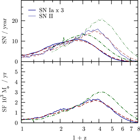
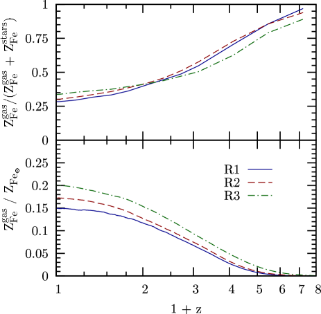
Figure 10: Left panel: the effect of resolution on the star formation rate (bottom) and supernova rates (top; tick lines: SNIa; thin lines: SNII). Right panel: the effect of resolution on the effect on the enrichment history. The upper panel shows the evolution of the fraction of Iron in contained in gas, while the lower panel shows the evolution of the Iron abundance in the gas. Solid, dashed and dot–dashed lines are for the R1, R2 and R3 runs, respectively.

First of all, by increasing resolution one better resolves processes, like “turbulent” gas motions and ram–pressure stripping, which are effective in diffusing metals away from the star forming regions, thus preventing them to be locked back in stars. Furthermore, the better–resolved and more wide–spread star formation at high redshift releases a larger fraction of metals in relatively shallower potential wells. Therefore, galactic winds are more efficient in distributing metals in the IGM.

As for the history of enrichment (right panel of Figure 10), we note that increasing resolution has the effect of progressively increasing the gas Iron abundance at all redshifts. While the overall effect is of about $\simeq 30$ per cent at $z=0$ it is by a factor of 2 or more at $z\raise-2.0pt\hbox{\hbox to0.0pt{\hbox{$\sim$}\hss}\raise 5.0pt\hbox{$>$}\ }4$. This illustrates that, while resolution has a modest, though sizable, effect at low redshift, it must be increased by a substantial factor to follow the enrichment process of the high–redshift IGM. As for the evolution of the fraction of Iron in gas, we note that it decreases with resolution at high redshift, while increasing at low redshift. The high–$z$ behaviour is consistent with the increasing star–formation efficiency with resolution, which locks back to stars a larger fraction of metals. On the other hand, at low redshift this trend is inverted (see also the right panel of Fig.9). This transition takes place at about the same redshift, $z\sim 2.5$, at which the star formation rate of the R3 run drops below that of the R1 runs, thus confirming the link between star–formation efficiency and locking of metals in stars.

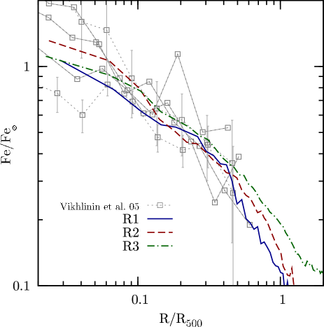
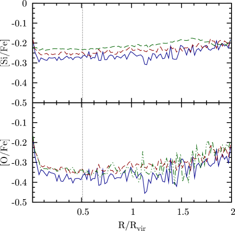
Figure 11: The effect of resolution on the abundance profiles of the Cl2 cluster. Left panel: profile of the mass–weighted Iron abundance, out to $R_{500}$. The observational data points in the left panel are the same as in Figure 8. Right panel: the profiles of the relative abundance of Silicon (top) and Oxygen (bottom) with respect to Iron, plotted out to 2$R_{\mathrm{vir}}$. The meaning of the different line types is the same as in the left panel of Figure 11. The dotted vertical line indicates the value of $R_{500}$.

An increased efficiency with resolution in distributing metals in the diffuse medium is also confirmed by the the Iron abundance profile (left panel of Figure 11). While we do not detect any obvious trend at small radii, $R\raise-2.0pt\hbox{\hbox to0.0pt{\hbox{$\sim$}\hss}\raise 5.0pt\hbox{$<$}\ }0.2R_{500}$, there is a clear trend for profiles to be become shallower at larger radii as resolution increases. In order to better show this effect, we plot in Figure 12 the Iron abundance profile out to 2$R_{\mathrm{vir}}$, by using linear scales for the cluster–centric distance. This allows us to emphasize the regime where the transition from the ICM to the high–density Warm-Hot Intergalactic Medium (WHIM) takes place (e.g., Cen & Ostriker, 2006). Quite interestingly, the effect of resolution becomes more apparent in the outskirts of clusters. Behind the virial radius, the abundance of Iron increases by 50 per cent from the low–resolution (LR) to the high–resolution (HR) runs. In these regions the effect of ram–pressure stripping is expected to be less important, owing to the lower pressure of the hot gas. This demonstrates that the increasing of the ICM metallicity with resolution is mainly driven by a more efficient ubiquitous high–redshift enrichment, rather than by ram-pressure stripping of enriched gas from merging galaxies.

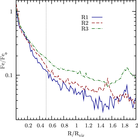
Figure 12: The effect of resolution on the profiles or Iron abundance, out to 2$R_{\mathrm{vir}}$. Linear scales are used for the radius, to emphasize the behaviour of the profiles in the cluster outskirts.

As for the profiles of the relative abundance (right panel of Fig. 11), they are rather flat out to $R_{\mathrm{vir}}$, with a relatively higher abundance for Silicon. In the innermost regions, the abundance ratios increase, with a more pronounced trend for [O/Fe]. The reason for this increase is an excess of recent star formation taking place at the cluster centre. As a consequence, elements mainly produced by short living stars, such as Oxygen, are released in excess with those, like Iron, which are mostly contributed by long–living stars. This also explains why the central increase is less apparent for [Si/Fe], being Silicon contributed by SNIa more than Oxygen is. An excess of star formation in the central regions of galaxy clusters is a well known problem of simulations, like those discussed here, which include only stellar feedback. For instance, Saro et al. (2006) analysed a set of simulations, similar to those presented here, to study the properties of the galaxy population. They concluded that the brightest cluster galaxies (BCGs) are always much bluer than observed, as a consequence of the low efficiency of SN feedback to regulate overcooling in the most massive galaxies.

In the outer regions, $R\raise-2.0pt\hbox{\hbox to0.0pt{\hbox{$\sim$}\hss}\raise 5.0pt\hbox{$>$}\ }$$R_{\mathrm{vir}}$, the two relative abundances tend to increase, again more apparently for Oxygen. The outskirts of galaxy clusters have been enriched at relatively higher redshift (see also discussion in Sect. 3.3.3, below), when the potential wells are shallower and the enrichment pattern tends to be more uniformly distributed. This causes the products of short–living stars to be more effectively distributed to the diffuse gas than at lower redshift. In this sense, the increasing trend of the relative abundances produced by short– and long–living stars represents the imprint of the different enrichment epochs. As for the dependence on resolution, we note a systematic trend for an increase of Oxygen and, to a lesser extent, of Silicon, at least for $R\raise-2.0pt\hbox{\hbox to0.0pt{\hbox{$\sim$}\hss}\raise 5.0pt\hbox{$>$}\ }0.1R_{500}$. This behaviour is consistent with the increased star formation rate at high redshift. Since Oxygen is relatively more contributed by short–living stars, then it is released at higher redshift than Iron and, therefore, has a more uniform distribution, an effect that increases with resolution. In the innermost cluster regions, $R\raise-2.0pt\hbox{\hbox to0.0pt{\hbox{$\sim$}\hss}\raise 5.0pt\hbox{$<$}\ }0.1R_{500}$, resolution acts in the direction of reducing the excess of Oxygen and Silicon. This can also be explained in terms of the dependence of the SFR on resolution: since most of the low–redshift SFR is concentrated at the cluster centre, its reduction at low redshift also reduces in these regions the relative amount of metals released from short–living stars.

In conclusion, our resolution study demonstrates that the general pattern of the ICM chemical enrichment is rather stable in the central regions of clusters, $R\raise-2.0pt\hbox{\hbox to0.0pt{\hbox{$\sim$}\hss}\raise 5.0pt\hbox{$<$}\ }0.3R_{500}$. However, the situation is quite different in the cluster outskirts, where both absolute and relative abundances significantly change with resolution, as a consequence of the different efficiency with which high–redshift star formation is described. On the one hand, this lack of numerical convergence becomes quite apparent on scales $\raise-2.0pt\hbox{\hbox to0.0pt{\hbox{$\sim$}\hss}\raise 5.0pt\hbox{$>$}\ }R_{500}$, which can be hardly probed by the present generation of X–ray telescopes. On the other hand, resolution clearly becomes important in the regime which is relevant for the study of the WHIM, which is one of the main scientific drives for X–ray telescopes of the next generation (e.g., Yoshikawa et al., 2004).

3.3 Changing the model of chemical evolution

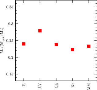
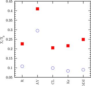
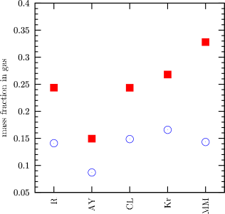
Figure 13: The same as in Figure 4, but changing parameters related to the model of chemical evolution and to the feedback. The labels indicating the different runs are as reported in Table 2.

3.3.1 The effect of the IMF

As already discussed in 2.3.4, a vivid debate exists in the literature as to whether the level of the ICM enrichment can be accounted for by a standard, Salpeter–like, IMF or rather requires a top–heavier shape. The absolute level of enrichment in one element, e.g. Iron, does not necessarily represent an unambiguous imprint of the IMF in our simulations. For instance, an exceedingly top–light IMF could still produce an acceptable Iron abundance in the presence of an excess of star formation in simulations. For this reason, it is generally believed that a more reliable signature of the IMF is provided by the relative abundances of elements which are produced by SNIa and SNII.

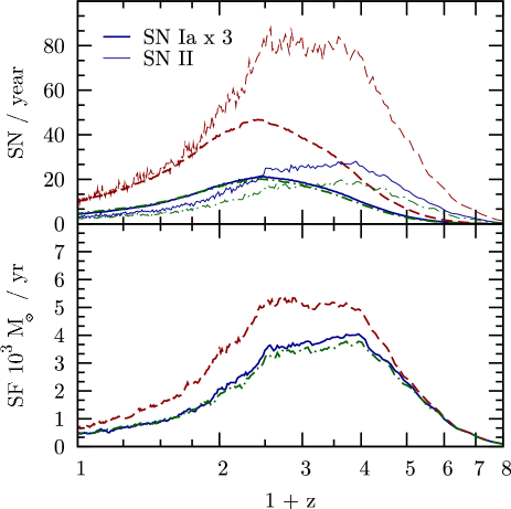
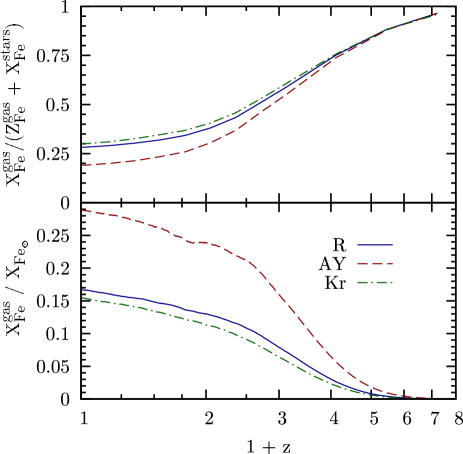
Figure 14: The same as Figure 6, but changing the IMF. The solid lines correspond to the reference run, while the short–dashed and the long–dashed lines are for the IMFs by Arimoto & Yoshii (1987) and by Kroupa (2001), respectively.

As shown in Figure 14 the effect of assuming an IMF, which is top–heavier than the Salpeter one, is that of significantly increasing the number of SNII and, to a lesser extent, also the number of SNIa. This is consistent with the plot of Fig. 3, which shows that an Arimoto–Yoshii IMF predicts more stars than the Salpeter one already for $M_{*}\simeq 1.5M_{\odot}$. The larger number of SN clearly generates a higher level of enrichment at all redshifts (bottom right panel of Fig. 14. A higher level of gas enrichment increases the cooling efficiency and, therefore, the star–formation rate (bottom left panel of 14). A higher star formation efficiency has, in turn, the effect of increasing the fraction of Iron which is locked in the stellar phase (top–right panel of 14).

In Figure 5 we show the maps of Iron abundance (left panels) and of the fractional enrichment from SNII for the three IMFs. The effect of a top–heavy IMF is confirmed to increase the overall level of enrichment in Iron. At the same time, the contribution of SNII becomes more important, thus consistent with the increase of the number of massive stars.

The effect of assuming a top–heavier IMF is quite apparent on the profiles of Iron abundance (left panel of Figure 15). The level of enrichment increases quite significantly, up to factor of two or more at $R\raise-2.0pt\hbox{\hbox to0.0pt{\hbox{$\sim$}\hss}\raise 5.0pt\hbox{$>$}\ }0.5R_{500}$, bringing it to a level in excess of the observed one. As expected, the larger fraction of core–collapse SN also impacts on the relative abundances (right panel of Fig. 15), especially for [O/Fe]. Since Oxygen is largely contributed by SNII, its relative abundance to Iron increases by about 60 per cent.

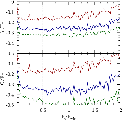
Figure 15: The effect of changing the IMF and the yields on the abundance profiles. Left panel: profiles of the mass–weighted Iron abundance. The data points are the same as in Figure 8. Right panel: the relative abundance of Silicon (top) and Oxygen (bottom) with respect to Iron, for the same runs shown in the left panel. The different line–types have the same meaning as in Figure 14.

This result goes in the direction of alleviating the tension between the largely sub–solar [O/Fe] values found for the Salpeter IMF and the nearly solar value reported by observational analyses (e.g., Tamura et al., 2004). However, an overestimate of Oxygen from the spectral fitting, used in the analysis of observational data, may arise as a consequence of a temperature–dependent pattern of enrichment. Rasia et al. (in preparation) analysed mock XMM–Newton observations of simulated clusters, including chemical enrichment with the purpose of quantifying possible biases in the measurement of ICM metallicity. As for the Iron abundance, they found that its emission–weighted definition is a good proxy of the spectroscopic value. On the contrary, the spectroscopic measurement of the Oxygen abundance turns out to be significantly biased high with the respect to the intrinsic abundance. The reason for this bias is that, unlike Iron, the Oxygen abundance is obtained from emission lines which are in the soft part of the spectrum. On the other hand, relatively colder structures such as filaments, seen in projection and surrounding the ICM, give a significant contribution to the soft tail of the spectrum. Since these structures are on average more enriched than the hot ICM, they are over–weighted when estimating element abundances from soft ($\raise-2.0pt\hbox{\hbox to0.0pt{\hbox{$\sim$}\hss}\raise 5.0pt\hbox{$<$}\ }1$ keV) transitions. This is the case of Oxygen, whose abundance is generally estimated from the O-VIII line, which is at about 0.65 keV.

Addressing the issue of observational biases in the measurement of the ICM enrichment is outside the scope of this paper. Still, the above example illustrates that such biases need definitely to be understood in detail if the enrichment pattern of the ICM has to be used as a fossil record of the past history of star formation in cluster galaxies.

As for the results based on the IMF by Kroupa (2001), we note that it induces only a small difference in the SFR with respect to the Salpeter IMF. While the SNIa rate is also left essentially unchanged, the SNII rate is now decreased by about 50 per cent. The reason for this is that the Kroupa IMF falls below the Salpeter one in the high mass end, $\raise-2.0pt\hbox{\hbox to0.0pt{\hbox{$\sim$}\hss}\raise 5.0pt\hbox{$>$}\ }5M_{\odot}$ (see Figure 3). This is consistent with the maps shown in the bottom panels of Fig. 5. The global pattern of Iron distribution is quite similar to that provided by the Salpeter IMF, while the relative contribution from SNII is significantly reduced. Consistent with this picture, the profile of the Iron abundance shown in Fig. 15 does not show an appreciable variation with respect to the reference case. On the contrary, the profile of the Oxygen abundance and, to a lesser extent, of Silicon abundance, decreases significantly.

Our results confirm that $[\alpha/Fe]$ relative abundances are sensitive probes of the IMF. However, we have also shown that different elements are spread in the ICM with different efficiencies. This is due to the fact that long–lived stars can release metals away from star forming regions and, therefore, their products have an enhanced probability to remain in the diffuse medium (see discussion in Sect. 3.1). Therefore, both a correct numerical modeling of such processes and an understanding of observational biases are required for a correct interpretation of observed metal content of the ICM.

3.3.2 Changing the yields

In Figure 16 we show the effect of using the yields by Chieffi & Limongi (2004) (CL) for the SNII, instead of those by Woosley & Weaver (1995) (WW) as in the reference run, on the Iron density profile. As for the enrichment pattern of the ICM, using either one of the two sets of yields gives quite similar results, both for the abundance of Iron and for the [O/Fe] relative abundance. This is apparently at variance with the results shown in Fig.2, where we have shown the differences in the production of different metals from an SSP for the two sets of yields. However, we note from that figure that such differences in the metal production have a non trivial dependence on the SSP characteristics, being different elements over– or under–produced for one set of yields, depending on the SSP initial metallicity. On the other hand, the metallicity of each star particle in the simulations depends on the redshift at which it is created, with the star–formation history being in turn affected by the enrichment pattern.

As for the enrichment in Iron (left panel of Fig. 16), we remind that this element is mostly contributed by SNIa, while the contribution from SNII is not only sub-dominant, but also preferentially locked back in stars. Since we are here changing the yields of the SNII, there is not much surprise that the effect of the profiles of $Z_{Fe}$ is marginal. The situation is in principle different for Oxygen (right panel of Fig.16). However, Fig.2 shows that the WW yields for Oxygen are in excess or in defect with respect to the CL ones, depending on the initial metallicity. As a result, we find that [O/Fe] for the diffuse gas is left again substantially unchanged, while a significant variation is found for stars, whose [O/Fe] is about 40 per cent larger when using the CL yields table. The profiles of [O/Fe] for stars show a mild decrease at large radii, consistent with the fact that Oxygen is more efficiently spread around stars in the regions where enrichment takes place at higher redshift (see discussion in Sect. 3.1). Once again, this difference in the enrichment pattern of gas and stars reflects the different efficiency that gas dynamical processes have in transporting metals away from star forming regions.

As a final remark, we would like to emphasize that several other tables of stellar yields have been presented in the literature, besides the ones by WW and CL considered here, which refer only to massive stars, and those by van den Hoek & Groenewegen (1997) and by Thielemann et al. (2003) that we adopted for low and intermediate mass stars and for SNIa, respectively. Besides the yields for intermediate–mass stars computed by Renzini & Voli (1981), other sets of metallicity–dependent yields have been provided by Iwamoto et al. (1999) and Marigo (2001) for intermediate and low–mass stars, and by Portinari et al. (1998) for massive stars. The differences among such sets of yields are due to the different stellar evolutionary tracks used and/or to the different way of describing the structure of the progenitor star. A different approach has been followed by François et al. (2004), who inferred stellar yields by requiring that their model of chemical evolution reproduces the observed enrichment pattern of the Milky Way.

Assessing in detail which one of them should be preferred to trace the cosmic evolution of metal production with hydrodynamical simulations is beyond the scopes of this paper. It is however clear that any uncertainty in the models on which yields computations are based can produce significant changes in the pattern the ICM enrichment (e.g., Gibson et al., 1997).

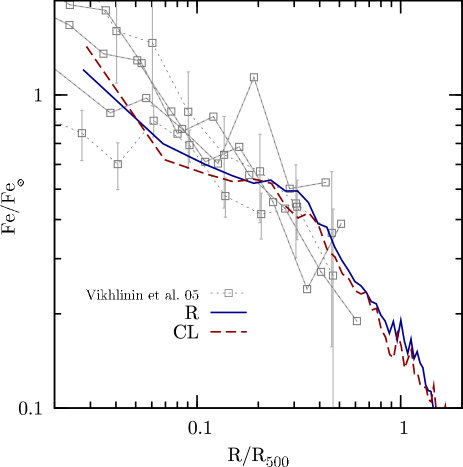
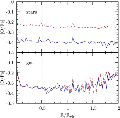
Figure 16: The effect of changing the SNII yields on the abundance profiles. Left panel: profile of the Fe abundance in the ICM; the data points are the same as in Figure 8. Right panel: the profiles of the [O/Fe] relative abundances for the ICM (lower panel) and for the stars (upper panel). Solid and dashed curves refer to the reference (R) run, based on the yields by Woosley & Weaver (1995), and to a run (CL) in which the yields by Chieffi & Limongi (2004) are used instead.

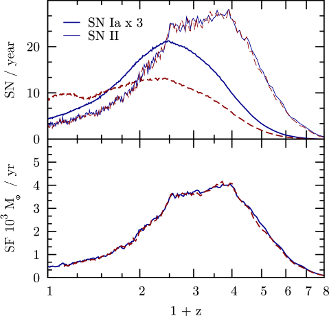
Figure 17: Left panel: the effect of changing the lifetime function on the star formation rate (bottom panel) and supernova rates (top panel; tick lines: SNIa; thin lines: SNII). The meaning of the different line types is the same as in the left panel of Figure 11. Right panel: the effect of the lifetime function on the profile of the Iron abundance (right panel). The data points are the same as in Figure 8. The solid line is for the reference (R) run, which uses the lifetime function by Padovani & Matteucci (1993), while the dashed line is for the MM run which uses the lifetime function by Maeder & Meynet (1989).

3.3.3 The effect of the lifetimes

As we have shown in Figure 1, using the lifetime function by Maeder & Meynet (1989), instead of that by Padovani & Matteucci (1993), corresponds to significantly increasing the delay time for the release of energy and metals from low–mass stars with $M\raise-2.0pt\hbox{\hbox to0.0pt{\hbox{$\sim$}\hss}\raise 5.0pt\hbox{$<$}\ }1M_{\odot}$, while leaving substantially unchaged that of massive stars. As a result, we expect that the SNII rate will remain substantially unchanged, while shifting towards lower redshift the rate of SNIa. This expectation is completely in line with the results shown in the left panel of Figure 17: changing the lifetime function has a small enough effect on the history of enrichment that the resulting SFR and SNII rate are left completely unchanged; on the other hand the SNIa rate is suppressed at high redshift, while it is substantially increased at $z\raise-2.0pt\hbox{\hbox to0.0pt{\hbox{$\sim$}\hss}\raise 5.0pt\hbox{$<$}\ }0.5$.

The consequence of changing the lifetimes on the typical epoch of the ICM enrichment can be can be appreciated from Fig. 18. To this purpose, we computed for each gas particle the mean value of the cosmic time at which it has been enriched. This quantity is obtained by weighting each epoch, at which an enrichment episode takes place, by the mass of metals received within that time–step. In Figure 18 we plot the radial profile of the mean cosmic epoch of enrichment, which is computed by averaging over all the gas particles falling inside different radial intervals. Outside the virial radius, for both lifetime functions the enrichment is progressively more pristine as we go to larger cluster-centric distances. While at $R_{\mathrm{vir}}$the mean redshift of enrichment is about 0.7, this increases to $\raise-2.0pt\hbox{\hbox to0.0pt{\hbox{$\sim$}\hss}\raise 5.0pt\hbox{$>$}\ }1.5$ at 2$R_{\mathrm{vir}}$. Quite interestingly, inside $\simeq 0.8$$R_{\mathrm{vir}}$the age of enrichment becomes nearly constant down to the central regions, $\sim 0.2$$R_{\mathrm{vir}}$. This change of behaviour further indicates that processes other than star formation, e.g. related to gas dynamical processes, become important in determining the enrichment pattern. In the core region, $\raise-2.0pt\hbox{\hbox to0.0pt{\hbox{$\sim$}\hss}\raise 5.0pt\hbox{$<$}\ }0.2$$R_{\mathrm{vir}}$, there is a sudden decrease of the enrichment redshift. This is due to the excess of recent star formation, which takes place in the central cluster galaxy, and which also causes the spike in the [O/Fe] relative abundance.

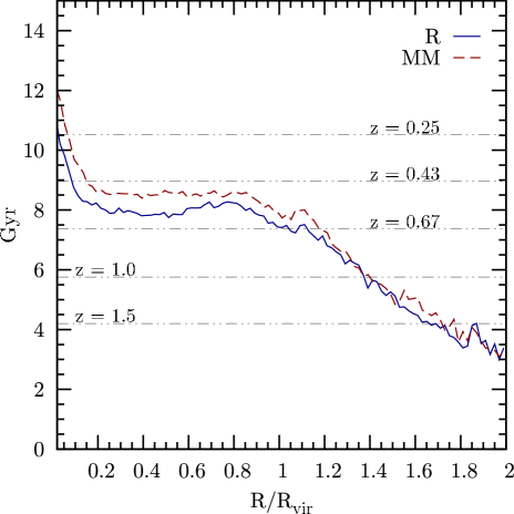
Figure 18: The radial dependence of the mean value of the age of the Universe at which the ICM has been enriched. The solid curve is for the reference (R) runs, which uses the lifetimes by Padovani & Matteucci (1993), while the dashed curve is when using the lifetimes by Maeder & Meynet (1989). Horizontal dashed lines indicate different values of redshift corresponding to difference cosmic times.

Using the lifetimes by Maeder & Meynet (1989) turns into a more recent enrichment of the ICM. We should remember here that this figure shown the mean age at which gas has been enriched in all metals. Since the global metallicity is dominated by Oxygen, mostly produced by SNII, we expect a more pronunced effect on the enrichment in Iron. In principle, a more recent enrichment due to longer delay times of SNIa could help explaining the observational evidences for an evolution of the ICM iron content at $z\raise-2.0pt\hbox{\hbox to0.0pt{\hbox{$\sim$}\hss}\raise 5.0pt\hbox{$<$}\ }0.5$ (Balestra et al., 2007). We will postpone a more detailed comparison with the observed ICM metallicity evolution to a forthcoming paper (Fabjan et al., in preparation).

As for the profile of the Iron abundance, we note that there is a small but sizeable increase, especially at small radii. This increase is due to a more efficient unlocking of Iron from star forming regions. Since the delay time is enhanced for SNIa, they have an larger probability to release metals outside star forming regions. On the other hand, we verified that the enrichment is Oxygen is left unchanged, as expected from the stability of the SNII rates. As a result, we find that [O/Fe] decreases by about 0.1 at $R_{500}$ and by 0.2 in the innermost regions.

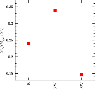
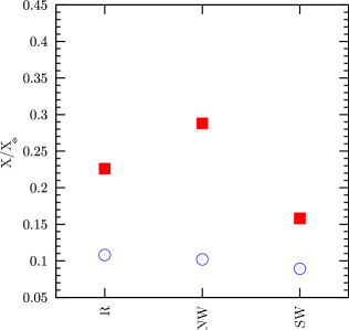
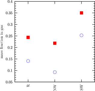
Figure 19: The same as in Figure 4, but changing the velocity of the galactic winds. The labels indicating the different runs are as reported in Table 2.

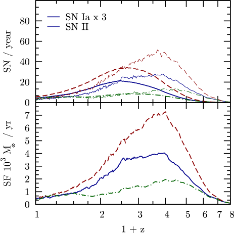
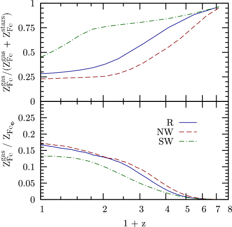
Figure 20: The same as Figure 6, but changing the feedback strength associated to galactic winds. The solid lines correspond to the reference run, while the short–dashed and the long–dashed lines are for the runs with strong winds (SW) and switching off winds (NW), respectively.

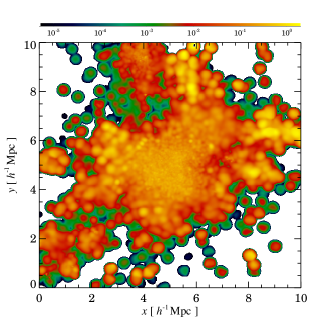
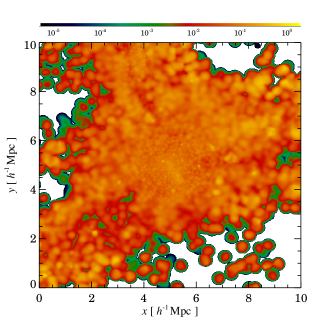
Figure 21: Maps of the Iron metallicity for the run with no winds (NW, left panel), for the reference run (R, central panel; $v_{w}=500\,{\rm km\,s^{-1}}$) and for the run with strong winds (SW, right panel; $v_{w}=1000\,{\rm km\,s^{-1}}$). Details of the maps are the same as in Fig.5.

3.3.4 Changing the feedback strength

Feedback from galactic winds has been originally implemented in the GADGET code with the purpose of preventing overcooling (Springel & Hernquist, 2003a) in simulations of galaxy formation. Besides producing a realistic star formation in cosmological simulations (Springel & Hernquist, 2003b), galactic winds are also expected to play a crucial role in the transport of metals outside star–forming regions and, therefore, in the enrichment of the diffuse gas. According to the implementation of galactic ejecta in the GADGET code, gas particles to be uploaded in winds are chosen among star forming particles which, by definition, are those more metal rich. Recent numerical studies of the key role played by winds in enriching diffuse cosmic baryons have been presented by Davé & Oppenheimer (2006), who focused their analysis on the high–redshift IGM, and by Cen & Ostriker (2006), who concentrated on the study of the WHIM.

The left panel of Figure 19 clearly shows that neglecting the effect of winds increases the star fraction in clusters up to $\sim 35$ per cent. This value is possibly even an underestimate, owing to the lack of numerical convergence of the star fraction in the absence of winds Borgani et al. (2006). On the other hand, increasing the wind speed to $1000\,{\rm km\,s^{-1}}$ reduces the fraction of cooled gas by almost a factor two. This reduction of the star fraction inside the cluster virial region at $z=0$ is just the consequence of the suppressed star formation due to the wind action (see the left panel of Figure 20). As shown in the right panel of Figure 19, an increasing wind efficiency also provides a more efficient distribution of metals in the gas. This is confirmed by the maps of Iron abundance shown in Figure 21. In the absence of winds, the pattern of the Iron distribution is quite patchy, with lumps of high abundance surrounding the star–forming regions. On the other hand, including the effect of winds turns into a more diffused enrichment pattern, an effect which increases with the winds’ speed.

As shown in the right panel of Fig. 19, this effect is more pronounced for Oxygen, whose mass fraction in gas increases by a factor of about 2.5, than for Iron, for which the same fraction increases by about 50 per cent. As already discussed, Iron is more efficiently distributed outside star–forming regions. This is due to the fact that Iron is largely contributed by long–lived stars, which explode when star particles possibly had the time to leave star–forming regions. Therefore, these regions are expected to be relatively more enriched in Oxygen. Since galactic winds are uploaded with gas from star–forming particles, they are relatively more enriched in Oxygen. As a consequence, increasing the feedback from winds has the general effect of increasing the diffusion of metals, by an amount which is larger for Oxygen than for Iron. This effect also explains why the ICM metallicity is not suppressed in the same proportion of star formation, when feedback from winds increases (see left and central panel of Fig. 19).

As shown in the right panel of Fig.20, the effect of winds in unlocking metals from stars is more effective at high redshift. This is quite expected, owing to the shallower potential wells which are present at earlier times and make winds more effective in transporting metals outside star–forming regions. This result further illustrate the fundamental role that winds have played in establishing the enrichment pattern of the high–redshift IGM (Davé & Oppenheimer, 2006).

The dependence of the abundance profiles on the feedback strength is shown in Figure 22. The effect of increasing the wind speed from $500\,{\rm km\,s^{-1}}$ to $1000\,{\rm km\,s^{-1}}$ is that of suppressing the profile of Iron abundance, as a consequence of the suppressed star formation, bringing it below the level indicated by observational data. On the other hand, the effect of neglecting galactic winds has a less direct interpretation. While for $R\raise-2.0pt\hbox{\hbox to0.0pt{\hbox{$\sim$}\hss}\raise 5.0pt\hbox{$>$}\ }0.3R_{500}$ the enrichment level is higher, due to the larger amount of stars, it falls below the profile of the reference (R) run at smaller radii, due to the reduced efficiency of metal transport. Only in the innermost regions, the excess of star formation, taking place in the absence of efficient feedback, causes a spike in the Iron abundance.

As for the profiles of the relative abundances of [O/Fe] and [Si/Fe] (right panel of Fig.22), they confirm the different effect that feedback has in determining the enrichment level for different elements. Consistent with what shown in Fig.19, Silicon and Oxygen becomes progressively over–abundant with respect to Iron as the feedback strength increases. In the innermost regions, the excess of low–redshift star formation in the absence of efficient feedback manifests itself through a sudden increase of the relative abundances. A comparison of this figure with the right panel of Fig.15 shows that the effect of a stronger feedback is similar to that induced by assuming a top–heavier IMF. This highlights once more that using the observational determination of the [$\alpha$/Fe] abundances to infer the IMF requires a good knowledge of other gas–dynamical effects.

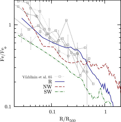
Figure 22: The effect of changing the feedback strength on the abundance profiles. The dot–dashed lines are for the run with strong winds (SW), while the dashes lines are for the run without winds (NW). Left panel: profiles of the mass–weighted Iron abundance. The data points are the same as in Figure 8. Right panel: the relative abundance of Silicon (top) and Oxygen (bottom) with respect to Iron, for the same runs shown in the left panel.

4 Discussion and conclusions

We presented results from hydrodynamical simulations of galaxy clusters, aimed at studying the metal enrichment of the Intra–Cluster Medium (ICM). Our simulations were based on a version of the Tree-SPH GADGET-2 code (Springel et al., 2001; Springel, 2005), which includes a detailed treatment of the production of metals from different stellar populations. In particular, we account for the delay times at which different stellar populations release energy and metals from SNIa and SNII explosions and stellar mass loss. The resulting chemo–dynamical code is rather flexible since it allows one to change the assumed stellar initial mass function (IMF), the life–time function and the tables of stellar yields. Thanks to the efficient implementation of the way in which the equations of the chemical evolution model are solved, the corresponding computational cost is only of about 10 per cent of the total cost of a simulation in a typical configuration.

The analyses presented in this paper have been carried out with the twofold aim of assessing in detail the impact of numerical effects and of changing the parameters defining the chemical evolution and the feedback model on the resulting pattern of ICM enrichment. For this reason, we have concentrated our analysis only on two medium poor clusters, having virial masses $M_{\rm vir}\simeq 2\times 10^{14}\,h^{-1}M_{\odot}$, which have been simulated in a variety of conditions. For this reason, we have preferred not to perform here any detailed comparison with observational X–ray data. Such a comparison would require simulations of a more extended set of clusters, so as to appreciate both the cluster-to-cluster variation of the enrichment pattern and the dependence on the cluster mass (Fabjan et al., in preparation).

The main results of our analysis can be summarized as follows.

(a)

Gas–dynamical effects, related to gas mixing, galactic winds and ram–pressure stripping, play an important role in determining the distribution and relative abundances of different chemical species. For instance, we find that the products of SNII are generally more concentrated around star–forming regions than those of low–mass stars, due to the different time–scales over which stars of different mass release metals. This emphasizes the relevance of properly including in the simulations a correct description of the lifetimes of different stellar populations.

(b)

A comparison with observed metallicity profiles obtained by Vikhlinin et al. (2005) from Chandra data shows a reasonable and encouraging agreement in both shape and normalization, when using a Salpeter (1955) IMF, within $\simeq 0.5R_{\rm vir}$. The [O/Fe] relative abundance is predicted to be undersolar, $\simeq-0.35$ over the cluster virial region, with a mild increase at larger radii and with a sudden increase in the core region, due to an excess of recent star formation.

(c)

For each gas particle we estimated the metallicity–weighted cosmic time of enrichment. We find that this typical age of enrichment of the hot gas corresponds to redshift $z\simeq 0.5$, over the whole cluster virial region. Only in the innermost region, which is heavily affected by the presence of the Brightest Cluster Galaxy (BCG), the enrichment took place at a significantly more recent epoch, due to an excess of low–redshift star formation.

(d)

As expected, the IMF has a strong impact on the enrichment level of both the ICM and the stellar populations. Assuming a top–heavy IMF (Arimoto & Yoshii, 1987), instead of the Salpeter (1955) one, it turns into an increase of the Iron abundance and of the [O/Fe] relative abundance. Within the cluster virial regions, the Iron metallicity of the ICM increases by almost a factor of two, while Oxygen increases by about a factor of three. Using the IMF proposed by Kroupa (2001), it turns into a general decrease of [O/Fe] with respect to the prediction of a Salpeter IMF, owing to the relatively smaller number of massive stars.

(e)

Increasing the velocity of galactic ejecta from $500\,{\rm km\,s^{-1}}$ to $1000\,{\rm km\,s^{-1}}$ provides a strong suppression of the star formation history and of the corresponding level of enrichment. The fraction of baryonic mass in stars within $R_{\rm vir}$ drops by about a factor of two, while the level of Iron enrichment drops only by about 40 per cent. This is due to the increasing efficiency of stronger winds to unlock metals from star–forming regions.

In order to judge the stability of our results against numerical effects, we have considered several different prescriptions to distribute metals around stars and the effect of progressively increasing resolution. For instance, we find that in the central regions, $R\raise-2.0pt\hbox{\hbox to0.0pt{\hbox{$\sim$}\hss}\raise 5.0pt\hbox{$<$}\ }0.3R_{500}$, the pattern of ICM enrichment is quite insensitive to the shape of the weighting kernel, to the number of neighbours over which metals are distributed. The only significant trend found is for the profiles of the Iron abundance to become higher at larger radii as the number of neighbors used for the spreading increases. As a general result, we can then conclude that our results are not strongly affected by the details with which metals are distributed around star–forming regions. Furthermore, we find no obvious trend in the Iron abundance profile with resolution within $0.3R_{500}$. However, we do find a significant and systematic increase of the enrichment level with resolution in the cluster outskirts: at $R\raise-2.0pt\hbox{\hbox to0.0pt{\hbox{$\sim$}\hss}\raise 5.0pt\hbox{$>$}\ }R_{\rm vir}$ the Iron abundance in the highest resolution run is about 60 per cent higher that in the low resolution run. These differences are not due to a lack of convergence of resolution of the total amount of stars found at $z=0$. Instead, they are mainly due to the better–resolved star formation at high redshift, which provides a more uniform enrichment of the inter–galactic medium (IGM). This calls for the need of significantly increasing the resolution to have numerically converged results on the enrichment pattern in the cluster outskirts and in the Warm-Hot Intergalactic Medium (WHIM).

The results presented in this paper and those from previous chemo–dynamical models of the ICM (e.g., see also Lia et al., 2002; Valdarnini, 2003; Sommer-Larsen et al., 2005) demonstrate that sophisticated models of chemical evolution can be efficiently included in advanced codes for cosmological simulations of galaxy clusters. This opens the possibility of accurately describing the history of metal production through cosmic epochs, in a variety of environments. While we have focused our analysis on the low–redshift enrichment of the ICM, a number of other studies can be foreseen, from the enrichment of the IGM at high redshift, $z\raise-2.0pt\hbox{\hbox to0.0pt{\hbox{$\sim$}\hss}\raise 5.0pt\hbox{$>$}\ }2$, to the metal abundances in both elliptical and disk galaxies (e.g., Kawata & Gibson, 2003; Kobayashi, 2004; Scannapieco et al., 2006).

Even restricting to the study of the ICM, a number of directions of further developments and improvements with respect to the analysis presented here can be devised.

As for the comparison with observational data, a fundamental step is represented by understanding in detail possible observational biases in the measurement of the ICM metallicity. In the analysis of observational data, the ICM metallicity is estimated by fitting the X–ray spectrum to a plasma model. On the other hand, in the analysis of simulations, metallicity is usually estimated by either mass–weighting or emission–weighting the metallicity carried by each gas particle. The best way of approaching this problem is by performing mock observations of simulated clusters, which reproduce as close as possible the observational setup (i.e., instrument response and PSF, instrumental background, etc.; Rasia et al., in preparation), and analyse them exactly in the same way as observational data. The preliminary comparison with observational data, presented in this paper, shows an encouraging agreement with the profiles of the Iron abundance as obtained from Chandra observations of a set of nearby relaxed clusters (Vikhlinin et al., 2005). As a word of caution, we point out that for a numerical model to be fully successful, it should reproduce at the same time the properties of the ICM and those of the cluster galaxy population. However, a well known problem of simulations based on stellar feedback, like those presented here, is that they produce central cluster galaxies which are much bluer and more star–forming than observed (e.g., Saro et al., 2006). In this respect, AGN feedback is generally considered as the most credible candidate to quench star formation at low redshift, thereby accounting for the observed properties of both the brightest cluster galaxies and of the “cool cores”. Besides regulating star formation, AGN feedback should also play an important role in distributing metals from the core regions, through the generation of buoyant bubbles created by collimated jets, which shock on the dense ambient gas (e.g., Dalla Vecchia et al., 2004; Sijacki & Springel, 2006a; Roediger et al., 2007, and references therein).

From the observational side, the sensitivity of the present generation of X–ray satellites are allowing us to measure the distribution of metals at most out to about $R_{500}$ for nearby, $z\sim 0.1$, clusters, while global measurement of the ICM metallicity are possible for distant cluster, out to $z\sim 1$ (e.g., Balestra et al., 2007). X–ray telescopes of the next generation, thanks to a much larger collecting area, improved spectral resolution and lower instrumental background, will open a new window on our knowledge of the chemo–dynamical history of the cosmic baryons. Deep pointings of distant clusters will provide the signature of the metal enrichment in the just–assembling ICM, out to $z\sim 2$, thus bridging the gap between observations of the metal–enrichment of the low–$z$ ICM and of the high–$z$ IGM. There is little doubt that numerical simulations, like those presented here, will provide the ideal tool for the interpretation of these observations within the framework of cosmological models of structure formation.

References

- Arimoto & Yoshii (1987) Arimoto N., Yoshii Y., 1987, A&A, 173, 23
- Balestra et al. (2007) Balestra I., Tozzi P., Ettori S., Rosati P., Borgani S., Norman V. M. C., Viola M., 2007, A&A, 462, 429
- Bate & Bonnell (2005) Bate M. R., Bonnell I. A., 2005, MNRAS, 356, 1201
- Baumgartner et al. (2005) Baumgartner W. H., Loewenstein M., Horner D. J., Mushotzky R. F., 2005, ApJ, 620, 680
- Bertelli et al. (1994) Bertelli G., Bressan A., Chiosi C., Fagotto F., Nasi E., 1994, A&AS, 106, 275
- Borgani et al. (2006) Borgani S., Dolag K., Murante G., Cheng L.-M., Springel V., Diaferio A., Moscardini L., Tormen G., Tornatore L., Tozzi P., 2006, MNRAS, 367, 1641
- Cen & Ostriker (2006) Cen R., Ostriker J. P., 2006, ApJ, 650, 560
- Chiappini et al. (1997) Chiappini C., Matteucci F., Gratton R., 1997, ApJ, 477, 765
- Chiappini et al. (2000) Chiappini C., Matteucci F., Padoan P., 2000, ApJ, 528, 711
- Chieffi & Limongi (2004) Chieffi A., Limongi M., 2004, ApJ, 608, 405
- Cora (2006) Cora S. A., 2006, MNRAS, 368, 1540
- Dalla Vecchia et al. (2004) Dalla Vecchia C., Bower R. G., Theuns T., Balogh M. L., Mazzotta P., Frenk C. S., 2004, MNRAS, 355, 995
- Davé & Oppenheimer (2006) Davé R., Oppenheimer B. D., 2006, ArXiv Astrophysics e-prints
- De Grandi et al. (2004) De Grandi S., Ettori S., Longhetti M., Molendi S., 2004, A&A, 419, 7
- De Lucia et al. (2004) De Lucia G., Kauffmann G., White S. D. M., 2004, MNRAS, 349, 1101
- Dolag et al. (2005) Dolag K., Vazza F., Brunetti G., Tormen G., 2005, MNRAS, 364, 753
- Domainko et al. (2006) Domainko W., Mair M., Kapferer W., van Kampen E., Kronberger T., Schindler S., Kimeswenger S., Ruffert M., Mangete O. E., 2006, A&A, 452, 795
- Finoguenov et al. (2002) Finoguenov A., Matsushita K., Böhringer H., Ikebe Y., Arnaud M., 2002, A&A, 381, 21
- Finoguenov & Ponman (1999) Finoguenov A., Ponman T. J., 1999, MNRAS, 305, 325
- François et al. (2004) François P., Matteucci F., Cayrel R., Spite M., Spite F., Chiappini C., 2004, A&A, 421, 613
- Gal-Yam et al. (2003) Gal-Yam A., Maoz D., Guhathakurta P., Filippenko A. V., 2003, AJ, 125, 1087
- Gal-Yam et al. (2002) Gal-Yam A., Maoz D., Sharon K., 2002, MNRAS, 332, 37
- Gastaldello & Molendi (2002) Gastaldello F., Molendi S., 2002, ApJ, 572, 160
- Gibson et al. (1997) Gibson B. K., Loewenstein M., Mushotzky R. F., 1997, MNRAS, 290, 623
- Greggio & Renzini (1983) Greggio L., Renzini A., 1983, A&A, 118, 217
- Haardt & Madau (1996) Haardt F., Madau P., 1996, ApJ, 461, 20
- Iwamoto et al. (1999) Iwamoto K., Brachwitz F., Nomoto K., Kishimoto N., Umeda H., Hix W. R., Thielemann F.-K., 1999, ApJS, 125, 439
- Katz et al. (1996) Katz N., Weinberg D. H., Hernquist L., 1996, ApJS, 105, 19
- Kawata & Gibson (2003) Kawata D., Gibson B. K., 2003, MNRAS, 340, 908
- Kay et al. (2002) Kay S. T., Pearce F. R., Frenk C. S., Jenkins A., 2002, MNRAS, 330, 113
- Kennicutt (1998) Kennicutt Jr. R. C., 1998, ApJ, 498, 541
- Kobayashi (2004) Kobayashi C., 2004, MNRAS, 347, 740
- Kravtsov et al. (2006) Kravtsov A. V., Vikhlinin A., Nagai D., 2006, ApJ, 650, 128
- Kroupa (2001) Kroupa P., 2001, MNRAS, 322, 231
- Larson (1998) Larson R. B., 1998, MNRAS, 301, 569
- Lia et al. (2002) Lia C., Portinari L., Carraro G., 2002, MNRAS, 330, 821
- Loewenstein & Mushotzky (1996) Loewenstein M., Mushotzky R. F., 1996, ApJ, 466, 695
- Maeder & Meynet (1989) Maeder A., Meynet G., 1989, A&A, 210, 155
- Maoz et al. (2005) Maoz D., Waxman E., Loeb A., 2005, ApJ, 632, 847
- Marigo (2001) Marigo P., 2001, A&A, 370, 194
- Matteucci (2003) Matteucci F., 2003, The Chemical Evolution of the Galaxy. The Chemical Evolution of the Galaxy. By Francesca Matteucci, Department of Astronomy, University of Trieste, Italy. Astrophysics and Space Science Library Volume 253 reprint Kluwer Academic Publishers, Dordrecht
- Matteucci & Gibson (1995) Matteucci F., Gibson B. K., 1995, A&A, 304, 11
- Matteucci & Greggio (1986) Matteucci F., Greggio L., 1986, A&A, 154, 279
- Matteucci & Recchi (2001) Matteucci F., Recchi S., 2001, ApJ, 558, 351
- Mazzotta et al. (2004) Mazzotta P., Rasia E., Moscardini L., Tormen G., 2004, MNRAS, 354, 10
- Monaco et al. (2006) Monaco P., Fontanot F., Taffoni G., 2006, ArXiv Astrophysics e-prints
- Mosconi et al. (2001) Mosconi M. B., Tissera P. B., Lambas D. G., Cora S. A., 2001, MNRAS, 325, 34
- Murante et al. (2004) Murante G., Arnaboldi M., Gerhard O., Borgani S., Cheng L. M., Diaferio A., Dolag K., Moscardini L., Tormen G., Tornatore L., Tozzi P., 2004, ApJ, 607, L83
- Mushotzky (2004) Mushotzky R. F., 2004, in Mulchaey J. S., Dressler A., Oemler A., eds, Clusters of Galaxies: Probes of Cosmological Structure and Galaxy Evolution Clusters of Galaxies: An X-ray Perspective. pp 123–+
- Nagashima et al. (2005) Nagashima M., Lacey C. G., Baugh C. M., Frenk C. S., Cole S., 2005, MNRAS, 358, 1247
- Navarro & White (1993) Navarro J. F., White S. D. M., 1993, MNRAS, 265, 271
- Padovani & Matteucci (1993) Padovani P., Matteucci F., 1993, ApJ, 416, 26
- Pipino et al. (2002) Pipino A., Matteucci F., Borgani S., Biviano A., 2002, New Astronomy, 7, 227
- Portinari et al. (1998) Portinari L., Chiosi C., Bressan A., 1998, A&A, 334, 505
- Portinari et al. (2004) Portinari L., Moretti A., Chiosi C., Sommer-Larsen J., 2004, ApJ, 604, 579
- Raiteri et al. (1996) Raiteri C. M., Villata M., Navarro J. F., 1996, A&A, 315, 105
- Rasia et al. (2006) Rasia E., Ettori S., Moscardini L., Mazzotta P., Borgani S., Dolag K., Tormen G., Cheng L. M., Diaferio A., 2006, MNRAS, 369, 2013
- Rebusco et al. (2005) Rebusco P., Churazov E., Böhringer H., Forman W., 2005, MNRAS, 359, 1041
- Recchi et al. (2001) Recchi S., Matteucci F., D’Ercole A., 2001, MNRAS, 322, 800
- Renzini (1997) Renzini A., 1997, ApJ, 488, 35
- Renzini (2004) Renzini A., 2004, in Mulchaey J. S., Dressler A., Oemler A., eds, Clusters of Galaxies: Probes of Cosmological Structure and Galaxy Evolution The Chemistry of Galaxy Clusters. pp 260–+
- Renzini & Voli (1981) Renzini A., Voli M., 1981, A&A, 94, 175
- Roediger et al. (2007) Roediger E., Brüggen M., Rebusco P., Böhringer H., Churazov E., 2007, MNRAS, 375, 15
- Romano et al. (2005) Romano D., Chiappini C., Matteucci F., Tosi M., 2005, A&A, 430, 491
- Romeo et al. (2006) Romeo A. D., Sommer-Larsen J., Portinari L., Antonuccio-Delogu V., 2006, MNRAS, 371, 548
- Rosati et al. (2002) Rosati P., Borgani S., Norman C., 2002, ARAA, 40, 539
- Salpeter (1955) Salpeter E. E., 1955, ApJ, 121, 161
- Samland (1998) Samland M., 1998, ApJ, 496, 155
- Sarazin (1988) Sarazin C. L., 1988, X-ray emission from clusters of galaxies. Cambridge University Press, Cambridge
- Saro et al. (2006) Saro A., Borgani S., Tornatore L., Dolag K., Murante G., Biviano A., Calura F., Charlot S., 2006, MNRAS, 373, 397
- Scalo (1986) Scalo J. M., 1986, Fundamentals of Cosmic Physics, 11, 1
- Scannapieco et al. (2005) Scannapieco C., Tissera P. B., White S. D. M., Springel V., 2005, MNRAS, 364, 552
- Scannapieco et al. (2006) Scannapieco C., Tissera P. B., White S. D. M., Springel V., 2006, MNRAS, 371, 1125
- Schmidt (1959) Schmidt M., 1959, ApJ, 129, 243
- Sijacki & Springel (2006a) Sijacki D., Springel V., 2006a, MNRAS, 366, 397
- Sijacki & Springel (2006b) Sijacki D., Springel V., 2006b, MNRAS, 371, 1025
- Sommer-Larsen et al. (2005) Sommer-Larsen J., Romeo A. D., Portinari L., 2005, MNRAS, 357, 478
- Springel (2005) Springel V., 2005, MNRAS, 364, 1105
- Springel et al. (2006) Springel V., Frenk C. S., White S. D. M., 2006, Nature, 440, 1137
- Springel & Hernquist (2002) Springel V., Hernquist L., 2002, MNRAS, 333, 649
- Springel & Hernquist (2003a) Springel V., Hernquist L., 2003a, MNRAS, 339, 289
- Springel & Hernquist (2003b) Springel V., Hernquist L., 2003b, MNRAS, 339, 312
- Springel et al. (2001) Springel V., Yoshida N., White S., 2001, New Astronomy, 6, 79
- Strickland & Heckman (2006) Strickland D. K., Heckman T. M., 2006, ArXiv Astrophysics e-prints
- Summers (1993) Summers F. J., 1993, PhD thesis, AA(California Univ.)
- Sutherland & Dopita (1993) Sutherland R. S., Dopita M. A., 1993, ApJS, 88, 253
- Tamura et al. (2004) Tamura T., Kaastra J. S., den Herder J. W. A., Bleeker J. A. M., Peterson J. R., 2004, A&A, 420, 135
- Theis et al. (1992) Theis C., Burkert A., Hensler G., 1992, A&A, 265, 465
- Thielemann et al. (2003) Thielemann F.-K., Argast D., Brachwitz F., Hix W. R., Höflich P., Liebendörfer M., Martinez-Pinedo G., Mezzacappa A., Panov I., Rauscher T., 2003, Nuclear Physics A, 718, 139
- Tormen et al. (1997) Tormen G., Bouchet F., White S., 1997, MNRAS, 286, 865
- Tornatore et al. (2004) Tornatore L., Borgani S., Matteucci F., Recchi S., Tozzi P., 2004, MNRAS, 349, L19
- Tutukov & Iungelson (1980) Tutukov A. V., Iungelson L. R., 1980, in Plavec M. J., Popper D. M., Ulrich R. K., eds, IAU Symp. 88: Close Binary Stars: Observations and Interpretation Statistical investigation of spectroscopic binary stars. pp 15–22
- Valdarnini (2003) Valdarnini R., 2003, MNRAS, 339, 1117
- van den Hoek & Groenewegen (1997) van den Hoek L. B., Groenewegen M. A. T., 1997, A&AS, 123, 305
- Vikhlinin (2006) Vikhlinin A., 2006, ApJ, 640, 710
- Vikhlinin et al. (2005) Vikhlinin A., Markevitch M., Murray S. S., Jones C., Forman W., Van Speybroeck L., 2005, ApJ, 628, 655
- Voit (2005) Voit G. M., 2005, Reviews of Modern Physics, 77, 207
- Woosley & Weaver (1995) Woosley S. E., Weaver T. A., 1995, ApJS, 101, 181
- Yoshikawa et al. (2004) Yoshikawa K., Dolag K., Suto Y., Sasaki S., Yamasaki N. Y., Ohashi T., Mitsuda K., Tawara Y., Fujimoto R., Furusho T., Furuzawa A., Ishida M., Ishisaki Y., Takei Y., 2004, PASJ, 56, 939