The tension of cosmological magnetic fields as a contribution to dark energy

We propose that cosmological magnetic fields generated in regions of finite spatial dimensions may manifest themselves in the global dynamics of the Universe as ‘dark energy’. We test our model in the context of spatially flat cosmological models by assuming that the Universe contains non-relativistic matter $\rho_{m}\propto\alpha^{-3}$, dark energy $\rho_{Q}\propto\alpha^{-3(1+w)}$, and an extra fluid with $\rho_{B}\propto\alpha^{n-3}$ that corresponds to the magnetic field. We place constraints on the main cosmological parameters of our model by combining the recent supernovae type Ia data and the differential ages of passively evolving galaxies. In particular, we find that the model which best reproduces the observational data when $\Omega_{m}=0.26$ is one with $\Omega_{B}\simeq 0.03$, $n\simeq 7.68$, $\Omega_{Q}\simeq 0.71$ and $w\simeq-0.8$.

1 Introduction

Recent advances in observational cosmology based on the analysis of a multitude of high quality observational data (type Ia supernovae, hereafter SNIa, cosmic microwave background, large scale structure, age of globular clusters, high redshift galaxies), strongly indicate that we are living in a flat ($\Omega=1)$ accelerating Universe containing a small baryonic component, non-baryonic cold dark matter needed to explain the clustering of extragalactic sources, and an extra component with negative pressure, usually called ‘dark energy’, needed to explain the present accelerated expansion of the Universe (eg. Riess et al. 1998; Perlmutter et al. 1999; Efstathiou et al. 2002; Caldwell 2002; Percival et al. 2002; Spergel et al. 2003; Tonry et al. 2003; Riess et al. 2004; Tegmark et al. 2004; Corasaniti et al. 2004).

From a theoretical point of view, various candidates for the exotic dark energy have been proposed, most of them characterized by an equation of state $p_{Q}=w\rho_{Q}$ with $w<-1/3$ (see Caldwell 2002; Peebles & Ratra 2003; Corasaniti et al. 2004 and references therein). A particular case of dark energy is the traditional $\Lambda$-model which corresponds to $w=-1$. Note that a redshift dependence of $w$ is also possible but present measurements are not precise enough to allow meaningful constraints (eg. Dicus & Repko 2004; Wang & Mukherjee 2006). From the observational point of view and for a flat geometry, a variety of studies, and especially the SNIa data, indicate that $w<-1$ (eg. Riess et al. 2004; Basilakos & Plionis 2005; Sanchez et al. 2006; Spergel et al. 2006; Wood-Vasey et al. 2007 and references therein). For such a fluid the condition $w<-1$ is problematic since it presents instabilities and causality problems (de la Macorra 2007). This may be considered as an indication that the dark energy interacts with another fluid, for example magnetic fields. Tsagas (2001) gave an interesting perspective to the problem by claiming that the effect of a primordial magnetic field may resemble that of dark energy through the coupling between the magnetic field and space time.

In the present paper, we would like to investigate the potential of present day large scale magnetic fields to account for the effect of dark energy in the observed acceleration of the expansion of the Universe. As we show in § 2, if the magnetic field is highly tangled, it cannot account for the cosmic tension implied by the presence of dark energy. On the other hand, we argue that, if the cosmic magnetic field is generated in sources whose overall dimensions remain unchanged during the expansion of the Universe, the stretching of this field by the expansion generates a tension that behaves as dark energy. In order to test our model, we introduce in § 3 an extra energy density term in the cosmological equations which we associate with the magnetic field. In § 4 we place constraints on the main parameters of our model by performing a join likelihood analysis utilizing the ‘gold sample’ of SNIa data (Riess et al. 2007) as well as the ages of the passively evolving galaxies (Simon et al. 2005). We conclude with a discussion on the possible values of cosmological magnetic fields in § 5.

2 Tension in a cosmological magnetic field

It is well known that a positive pressure in the expanding cosmic fluid contributes to the deceleration of the expansion. It is easy to understand this when we realize that every expanding part of the Universe is pushed against the expansion by its neighboring parts. As a result, each expanding part performs work against its surroundings, and thus loses kinetic energy. The exact opposite takes place when the expanding fluid feels a tension force. In that case, each expanding part is pulled outwards by its neighbors, and the work done on it by its neighbors contributes to the acceleration of its expansion (e.g. Harwit 1982). Dark energy is, therefore, the cosmic tension that accounts for the observed present accelerated expansion of the Universe.

When one talks about tension, one immediately comes to think about magnetic fields. Magnetic field lines may be considered as strained ropes, with a highly anisotropic pattern of tension and pressure. We do observe magnetic fields up to several tens of $\mu G$ in galaxy clusters (see Carilli & Taylor 2002 for a review), but their origin remains a mystery. There is a general belief that cosmic magnetic fields are produced through some type of dynamo process that amplified a weak protogalactic seed magnetic field of the order of $10^{-20}$ G (e.g. Ruzmaikin, Shukurov & Sokoloff (1988); Kulsrud et al. (1997)). In this picture, the magnetic field permeates the cosmic fluid which is assumed highly conductive. In other words, the sources of the cosmic magnetic field are electric currents distributed more or less isotropically throughout the expanding cosmic fluid. Furthermore, because of flux conservation, the magnetic field scales with the expansion of the Universe as $\alpha^{-2}$, where $\alpha$ is the Universe scale factor, and therefore, the magnetic energy contained in any expanding volume of the Universe scales as $\alpha^{-1}$. Such a magnetic field generates a positive isotropic (on average) pressure $p_{B}=\rho_{B}/3$, and $\rho_{B}\equiv B^{2}/8\pi\propto\alpha^{-4}$. The same result may be obtained after averaging out the magnetic pressure and tension terms. In other words, the equation of state of a highly tangled magnetic field is the same as that obtained for a fluid of highly relativistic particles, and therefore, it cannot account for the cosmic tension implied by the presence of dark energy. The above led the community to conclude that isotropic tension, or equivalently negative pressure, is peculiar to a scalar field (Zeldovich (1986)).

Here, we would like to investigate the potential of a different scenario in which the magnetic tension does manifest itself in the expansion of the Universe as dark energy. We thus propose that the sources of cosmological magnetic fields are of finite dimensions, and that these dimensions remain unchanged during the expansion of the Universe. It is interesting to note that, galaxy clusters are the largest gravitationally bound structures in the Universe and as such, they have decoupled from the background expansion. What we have in mind here is some mechanism that results in the generation of magnetic fields of order $B_{0}$ around ‘sources’ of spatial dimensions $r_{0}$ (such as galaxies, or clusters of galaxies). Such a scenario may not be unreasonable. In fact, we have already proposed a physical picture where magnetic fields are generated without the need for a dynamo mechanism, through the Poynting-Robertson effect on electrons in a highly conducting plasma around bright gravitating sources such as active galactic nuclei, black holes, neutron stars, and protostars (Contopoulos & Kazanas (1998); Contopoulos, Kazanas & Christodoulou (2006)).

If we assume the existence of such sources of cosmic magnetic fields, it is natural to further assume that the magnetic field around each source has a dipolar structure. In that case, the magnetic field drops with distance $r$ as

$$B(r)\approx B_{0}\left(\frac{r}{r_{0}}\right)^{-3}$$ (1)

in the region influenced by a source of size $r_{0}$ at its center. We argue that the Universe may be filled with several such expanding regions of comoving size $R\alpha(t)$, which contain cosmic magnetic sources of size $r_{0}\ll R\alpha$. The magnetic field energy in each such region is equal to

$$E_{B}=\int_{r=r_{0}}^{R\alpha}\frac{B^{2}(r)}{8\pi}4\pi r^{2}{\rm d}r\approx\frac{B_{0}^{2}r_{0}^{3}}{6}.$$ (2)

Obviously, the expansion of the Universe will gradually stretch each dipolar configuration described by eq. (1) into a monopolar configuration described by

$$B(r)\rightarrow B_{0}\left(\frac{r}{r_{0}}\right)^{-2}$$ (3)

in the region around each source. The magnetic field energy in the expanding region will approach the value

$$E_{B}=\int_{r=r_{0}}^{R\alpha}\frac{B^{2}(r)}{8\pi}4\pi r^{2}{\rm d}r\rightarrow\frac{B_{0}^{2}r_{0}^{3}}{2}\ ,$$ (4)

which is 3 times larger than the expression in eq. (2)!

We showed here that the magnetic energy $E_{B}$ contained inside a region of size $R\alpha(t)$ increases with increasing $\alpha$. This may be parametrized around the present epoch with a simple power law

$$E_{B}=fB_{0}^{2}r_{0}^{3}\alpha^{n}\ ,$$ (5)

where, $f\sim 1/3$, and $n$ is a positive parameter to be determined from observations (see § 4). As a result,

$$\rho_{B}=\left(\frac{3f}{4\pi}\right)B_{0}^{2}\left(\frac{r_{0}}{R}\right)^{3}\alpha^{n-3}\ ,\;\;\mbox{and}$$ (6)

$$p_{B}=-\frac{n}{3}\rho_{B}\ .$$ (7)

Note that in our picture, the magnetic field $B_{0}$ is not primordial, because if that were the case, by the time the Universe doubles its size, the magnetic field in each region of magnetic influence will have effectively completely transformed itself from purely dipolar to purely (split) monopolar. When that happens, the magnetic field contribution to the cosmological tension dies out. In our scenario, we expect that the physical mechanism responsible for the generation of the cosmic magnetic field (e.g. Contopoulos & Kazanas 1998) requires a certain number of years $\tau$ in order to build a value of the order of $B_{0}$.

3 Cosmological evolution

We test our hypothesis by introducing an extra term that accounts for the magnetic field in the standard cosmological equations. In particular, we assume that the Universe is homogeneous, isotropic, flat, and consists of the following three components denoted by subscripts ‘$m$’, ‘$Q$’ and ‘$B$’ respectively: non-relativistic matter (with zero pressure), an exotic fluid (dark energy), and a magnetic fluid with an equation of state given by eq. (7). The corresponding equation of state parameters $w\equiv p_{Q}/\rho_{Q}$ and $n\equiv-3p_{B}/\rho_{B}$ are assumed here for simplicity to be constant. Therefore, the evolution of the fluid densities $\rho_{m}$, $\rho_{Q}$ and $\rho_{B}$ is given by $\dot{\rho}_{m}=-3H\rho_{m}$, $\dot{\rho}_{Q}=-3(w+1)H\rho_{Q}$ and $\dot{\rho}_{B}=(n-3)H\rho_{B}$. The scale factor of the Universe $\alpha(t)$ evolves according to the Friedmann equation:

$$H^{2}\equiv\left(\frac{\dot{\alpha}}{\alpha}\right)^{2}=\frac{8\pi G}{3}(\rho_{m}+\rho_{Q}+\rho_{B})\ .$$ (8)

Differentiating the Friedman equation and using at the same time the above formalism we obtain

$$\frac{\ddot{\alpha}}{\alpha}=-\frac{4\pi G}{3}[\rho_{m}+(3w+1)\rho_{Q}+(-n+1)\rho_{B}]\;\;.$$ (9)

In this framework, we define the density parameters $\Omega_{m}(\alpha)$, $\Omega_{Q}(\alpha)$ and $\Omega_{B}(\alpha)$ as

$$\Omega_{m}(\alpha)\equiv\frac{\rho_{m}}{\rho_{m}+\rho_{Q}+\rho_{B}}\equiv\frac{\Omega_{m}\alpha^{-3}}{E^{2}(\alpha)}\ ,$$

$$\Omega_{Q}(\alpha)\equiv\frac{\rho_{Q}}{\rho_{m}+\rho_{Q}+\rho_{B}}\equiv\frac{\Omega_{Q}\alpha^{-3(1+w)}}{E^{2}(\alpha)}\ ,$$

$$\Omega_{B}(\alpha)\equiv\frac{\rho_{B}}{\rho_{m}+\rho_{Q}+\rho_{B}}\equiv\frac{\Omega_{B}\alpha^{-3+n}}{E^{2}(\alpha)}\ ,$$

with

$$E(\alpha)=\left(\Omega_{m}\alpha^{-3}+\Omega_{Q}\alpha^{-3(1+w)}+\Omega_{B}\alpha^{-3+n}\right)^{1/2}\ .$$ (10)

Here, the Hubble parameter is given by $H(\alpha)=H_{0}E(\alpha)$, where $H_{0}$ is the Hubble constant at the present time. Also, $\Omega_{m}+\Omega_{Q}+\Omega_{B}=1$.

Note that in the context of our model, $\Lambda$-models correspond to $(w,\rho_{B})=(-1,0)$ or $(n,\rho_{Q})=(3,0)$, while if $n=0$ or $w=0$, the extra fluid behaves like pressureless matter. It is interesting to mention that the interplay between the values of $w$ and $n$ could yield flat cosmological models for which there is not a one-to-one correspondence between the global geometry and the expansion of the Universe. Indeed, in a flat low-$\Omega_{m}$ model with $(w,n)=(-1/3,1)$ we have the same dynamics as in an open Universe, despite the fact that these models have a spatially flat geometry!

In this cosmological scenario, there is an epoch which corresponds to a value of $\alpha=\alpha_{I}$, where $\ddot{\alpha_{I}}=0$. This is called the inflection point. After that epoch we reach an acceleration phase with $\ddot{\alpha}>0$. Eq. (9) thus implies that at the inflection point,

$$\rho_{m,I}+(3w+1)\rho_{Q,I}+(-n+1)\rho_{B,I}=0\ ,$$ (11)

or

$$\Omega_{m}+\Omega_{Q}(3w+1)\alpha^{-3w}_{I}+\Omega_{B}(-n+1)\alpha^{n}_{I}=0\;\;.$$ (12)

Therefore, in order for the latter equation to contain roots in the interval of $\alpha\in[0,1]$, we obtain a theoretical boundary for the possible $(n,w_{Q})$ values, namely

$$3w\Omega_{Q}-n\Omega_{B}<-1\;\;{\rm with}\;\;w<0\;\;{\rm and}\;\;n>0\ .$$ (13)

It is obvious that when $\Omega_{B}\rightarrow 0$, the above constraint tends to the Quintessence case $w<-1/3$, as it should.

4 Likelihood Analysis

In order to constrain the cosmological parameters in our model, we use the ‘gold’ sample of 182 supernovae of Riess et al. 2007. In particular, we define the likelihood estimator as: ${\cal L}^{\rm SNIa}({\bf c})\propto{\rm exp}[-\chi^{2}_{\rm SNIa}({\bf c})/2]$ with:

$$\chi^{2}_{\rm SNIa}({\bf c})=\sum_{i=1}^{182}\left[\frac{{\cal M}^{\rm th}(z_{i},{\bf c})-{\cal M}^{\rm obs}(z_{i})}{\sigma_{i}}\right]^{2}\;\;.$$ (14)

where ${\cal M}$ is the distance modulus ${\cal M}=5{\rm log}D_{\rm L}+25$, $D_{\rm L}(z)$ is the luminosity distance $D_{\rm L}(z)=(1+z)x(z)$, $z_{i}$ is the observed redshift, $\sigma_{i}$ is the observed uncertainty, and ${\bf c}$ is a vector containing the cosmological parameters that we want to fit (Riess et al. 2007). Note, that $x$ is the coordinate distance related to the redshift through

$$x(z)=\frac{c}{H_{0}}\int_{0}^{z}\frac{{\rm d}y}{E(y)}\;\;.$$ (15)

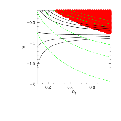
Figure 1: Likelihood contours in the $(\Omega_{Q},w)$ plane for $\Omega_{m}=0.26$. The contours are plotted where $-2{\rm ln}{\cal L}/{\cal L}_{\rm max}$ is equal to 2.30, 6.16 and 11.83, corresponding to 1$\sigma$, 2$\sigma$ and 3$\sigma$ confidence level. Note that the continuous and the dashed lines correspond to the SNIa and $H(z)$ results respectively, while the shadowed area is ruled out by stellar ages.

We remind the reader that we work here within the framework of flat cosmology ($\Omega_{m}+\Omega_{Q}+\Omega_{B}=1$) with non-zero large scale magnetic fields $\Omega_{B}\geq 0$. Furthermore, we use the results of the HST key project (Freedman et al. 2001) and fix the Hubble parameter to its nominal value $H_{0}\simeq 72$ km/s/Mpc. The matter density $\Omega_{m}$ remains the most weakly constrained cosmological parameter. In principle, $\Omega_{m}$ is constrained by the maximum likelihood fit to the WMAP and SNIa data, but in the spirit of this work, we want to use measures which are completely independent of the dark energy component. An estimate of $\Omega_{m}$ without conventional priors is not an easy task in observational cosmology. However, many authors using mainly large scale structure studies, have tried to put constraints to the $\Omega_{m}$ parameter. In particular, from the analysis of the power spectrum, Sanchez et al. (2006 and references therein) obtain a value $\Omega_{m}\simeq 0.24$. Moreover, Feldman et al. 2003 and Mohayee & Tully 2005 analyze the peculiar velocity field in the local Universe and obtain the values $\Omega_{m}\simeq 0.3$ and $\simeq 0.22$ respectively. In addition, Andernach et al. 2005, based on the cluster mass-to-light ratio, claim that $\Omega_{m}$ lies in the interval $0.15-0.26$ (see Schindler 2002 for a review). In the present paper, we decided to fix $\Omega_{m}$ to the value $0.26$.

In this case, the vector of unknown cosmological parameters is ${\bf c}\equiv(\Omega_{Q},w,n)$. We, therefore, sample the various parameters as follows: the dark energy density $\Omega_{Q}\in[0.01,0.74]$ in steps of 0.01, the dark energy parameter $w\in[-4,-0.1]$ in steps of 0.02, and the magnetic field scaling parameter $n\in[0.1,10]$ in steps of 0.02. Doing so, the likelihood function peaks at $\Omega_{Q}\simeq 0.5$ ($\Omega_{B}\simeq 0.24$) with $w\simeq-1.32$ and $n\simeq 0.44$ (or $w_{B}\simeq-0.15$) which corresponds to an age of the Universe of 12.3 Gyr. The latter appears to be ruled out by stellar ages. Indeed, in order to put further constraints on our solutions we use additionally the so called age limit, given by the age of the oldest globular clusters in our Galaxy ($\simeq 12.5-13$ Gyr; Caputo, Castellani & Quatra 1988; Cayrel et al. 2001; Hansen 2002 and 2004; Krauss 2003 and references therein). Taking into account the above age limit, the resulting best fit solution is: $\Omega_{B}\simeq 0.04$ ($\Omega_{Q}\simeq 0.7$), $w\simeq-0.8$ and $n\simeq 2.52$ (or $w_{B}\simeq-0.84$), corresponding to an age of 13.1 Gyr.

Figure 2: Left panel: We show the effective equation of state parameter as a function of the scale factor of the Universe. Right panel: We present the evolution of the density parameters $\Omega_{m}$ (solid), $\Omega_{Q}$ (dot-dashed) and $\Omega_{B}$ (dashed). The vertical lines corresponds to the present epoch.

In fig.1 (solid lines) we present the 1$\sigma$, 2$\sigma$ and $3\sigma$ confidence levels in the $(\Omega_{Q},w)$ plane by marginalizing over $n$. It is evident that $\Omega_{Q}$ is degenerate with respect to $w$ and that all the values in the interval $0\leq\Omega_{Q}\leq 0.74$ are acceptable within the $1\sigma$ uncertainty. Therefore, in order to put further constraints on $\Omega_{Q}$ we additionally use measures of $H(z)$ (see Simon et al. 2005) from the differential ages of passively evolving galaxies (hereafter $H(z)$ data). Note that the sample contains 9 entries. Doing so, the $H(z)$ likelihood function can be written as: ${\cal L}^{H}({\bf c})\propto{\rm exp}[-\chi^{2}_{H}({\bf c})/2]$ with:

$$\chi^{2}_{H}({\bf c})=\sum_{i=1}^{9}\left[\frac{H^{\rm th}(z_{i},{\bf c})-H^{\rm obs}(z_{i})}{\sigma_{i}}\right]^{2}\;\;,$$ (16)

where $H(z)$ is the Hubble parameter (see section 3), $H(z)=H_{0}E(z)$. The dashed lines in fig. 1 represents the $1\sigma$, $2\sigma$, and $3\sigma$, confidence levels in the $(\Omega_{Q},w)$ plane. In this case, we find that the best fit solution is $\Omega_{Q}\simeq 0.56$ ($\Omega_{B}\simeq 0.18$), $w\simeq-0.68$, and $n\simeq 8$ (with $T\simeq 13.2$Gyr). We now join the likelihoods,

$${\cal L}^{\rm joint}({\bf c})={\cal L}^{SNIa}\times{\cal L}^{H}\;\;,$$

and the overall function peaks at $\Omega_{Q}=0.71^{+0.03}_{-0.26}$ ($\Omega_{B}\simeq 0.03)$, $w=-0.80^{+0.14}_{-0.04}$ and $n\simeq 7.68^{+2.42}_{-4.00}$ (or $w_{B}\simeq-2.56$). Note that, the corresponding age of the Universe is $13.2$Gyr, while solving numerically eq. (12) the inflection point is at $\alpha_{I}\simeq 0.57$ (or $z_{I}\simeq 0.76$). Finally, due to the fact that the association of the extra term in the Friedman equation with the magnetic field is arbitrary, we may equally well consider the solution $\Omega_{B}\simeq 0.71$ ($\Omega_{Q}\simeq 0.03$), $w\simeq-2.56$ and $n\simeq 2.4$ (or $w_{B}\simeq-0.8$).

5 Discussion

The above values of $\Omega_{B}$ correspond to an average cosmic magnetic field

$$\langle B\rangle=(8\pi\Omega_{B}\rho_{cr}c^{2})^{1/2}\approx 650\Omega_{B}^{1/2}h\;\mu G\ ,$$ (17)

where, $\rho_{cr}\simeq 1.88\times 10^{-29}h^{2}\;\mbox{g}\ \mbox{cm}^{-3}$ is the critical density of the Universe; $h$ is the Hubble constant in units of 100 km/s/Mpc; and $c$ is the speed of light. If $\Omega_{B}\simeq 0.03$, $\langle B\rangle\simeq 80\mu G$, whereas if $\Omega_{B}\simeq 0.71$, $\langle B\rangle\simeq 400\mu G$. In the present work we do not discuss what physical mechanism may account for the generation of such high magnetic fields. Magnetic fields of the order of several tens of $\mu G$ have been observed in the centers of cooling flow clusters. We refer the reader to Vogt & Enßlin (2003) (and references therein) for a detailed discussion of the techniques used to estimate such high values of cluster magnetic fields. Furthermore, a number of authors have investigated the possibility that $\sim 50\mu G$ fields may provide magnetic pressure support in cluster atmospheres (e.g. Loeb & Mao 1994; Miralda-Escude & Babul 1995; Dolag & Schindler 2000; but see also Rudnick & Blundell 2003). We argued that dark energy (or equivalently cosmic tension) manifests itself as a tension agent between galaxy clusters, and as such, it obviously acts in intra-cluster space. Moreover, there is a theoretical indication that strong magnetic fields lie in regions of significantly reduced plasma density (e.g. Gazzola et al. 2007), which would make observations of cosmic magnetic fields through Farady rotation or X-ray emission in intra-cluster cosmic voids very difficult. We must keep in mind that the study of cosmic magnetic fields on scales of clusters of galaxies is a fairly new area of research (see Carilli & Taylor 2002 for a review), and therefore, we cannot preclude future observational surprises. In particular, any observation of magnetic fields of the order of $100\mu G$ over cosmological scales would give credence to our scenario.

We would like to end this section with a short discussion on the equation of state of the dark energy. As we mentioned in the introduction, there is strong indication for an equation of state more complicated than the simple assumption of a constant ratio between the pressure and the energy density. We may thus combine our two dark energy fluids into one with an effective dark energy parameter

$$w_{\rm eff}=\frac{P_{\rm eff}}{\rho_{\rm eff}}=\frac{P_{Q}+P_{B}}{\rho_{Q}+\rho_{B}}\;\;.$$ (18)

Using the evolution of $\rho_{Q}$ and $\rho_{B}$ the effective dark energy parameter as a function of time is given by

$$w_{\rm eff}(\alpha)=\frac{3w-n\nu\alpha^{3w+n}}{3(1+\nu\alpha^{3w+n})}\;\;\;\;{\rm where}\;\;\;\;\nu=\frac{\Omega_{B}}{\Omega_{Q}}\;\;.$$ (19)

Using our best fit parameters, $w_{\rm eff}\sim-0.9$ for $\alpha\sim 1$, $w_{\rm eff}\sim-0.8$ in the limit $\alpha\ll 1$, and $w_{\rm eff}\sim-2.6$ in the limit $\alpha\gg 1$. In the left panel of fig. 2, the solid line shows the evolution of the effective equation of state parameter as a function of the Universe scale factor. A first order Taylor expansion around the present epoch (Linder 2003) yields

$$w_{\rm eff}(\alpha)\simeq-0.87+0.36(1-\alpha)\;\;.$$ (20)

In the right panel of fig. 2 we show the evolution of the density parameters $\Omega_{m}$ (solid line), $\Omega_{Q}$ (dot-dashed) and $\Omega_{B}$ (dashed). It is interesting that, although at the present time the dark energy in dominant, before the inflection point ($\alpha_{I}\simeq 0.57$) the Universe was matter dominated, i.e. $\Omega_{m}(\alpha\ll 1)\approx 1$. In fact, we estimate that prior to the inflection point, $\Omega_{B}\leq 0.2\%\Omega_{m}$, which corresponds to an average cosmic magnetic field $\langle B\rangle\leq 30\mu G$. This value was well under equipartition, and therefore, one may argue that, at an early enough epoch, matter is able to generate the cosmological magnetic fields required in our scenario (for example, through the Poynting-Robertson mechanism described in Contopoulos & Kazanas 1998).

We conclude with a summary of the main elements of our scenario:

1. The cosmological magnetic field is generated in sources of characteristic size $r_{0}$ with characteristic value $B_{0}$. The main idea is that the size of these sources does not follow the overall expansion of the Universe. We know that the expansion of the Universe manifests itself over length scales larger than the typical size of clusters of galaxies. This leads us to suggest that the size of our putative magnetic field sources is of the order of a few Mpc.

2. Each source is associated with a region of magnetic influence around it where the large scale field is due to the central source. The sources are uniformly and isotropically distributed throughout the Universe.

3. As the Universe expands, the magnetic field in each region of influence is stretched, and the total magnetic field energy grows. This results in the acceleration of the expansion. The acceleration will decrease unless new sources are continuously generated throughout the Universe.

4. We model the effect of the magnetic field with an extra term $\rho_{B}\propto\alpha^{n-3}$ in the Freedman equations. The model that best reproduces the observational data when $\Omega_{m}=0.26$ is one with $\Omega_{B}\simeq 0.03$, $n\simeq 7.68$, $\Omega_{Q}\simeq 0.71$ and $w\simeq-0.8$, which yields an average cosmic magnetic field of the order of $\sim 80\mu G$. Obviously, we may equally well consider the solution $\Omega_{B}\simeq 0.71$, $n\simeq 2.4$, $\Omega_{Q}\simeq 0.03$ and $w\simeq-2.56$. The latter corresponds to an average cosmic magnetic field of the order of $\sim 400\mu G$.

References

- (1) Andernach, H., Plionis, M., Lopez-Cruz, O., Tago, E., Basilakos, S., 2005, Astronomical Society of the Pacific Conference Series, vol. 329, p. 289-293. Nearby Large-Scale Structures and the Zone of Avoidance, Proceedings of a meeting held in Cape Town, South Africa, March 28 – April 2, 2004, San Francisco: Astronomical Society of the Pacific, 2005.
- (2) Basilakos, S. & Plionis, M., 2005, MNRAS, 360, L35
- (3) Caldwell, R. R., 2002, Physics Letters B, 545, 23
- (4) Caputo, F., Castellani, V., Quarta, M. L, 1988, A Self-Consistent Approach to the Age of Globular Cluster M15, The Early Universe: Reprints Edited by Edward W. Kolb and Michael S. Turner. Frontiers in Physics, Reading: Addison-Wesley, p.263
- (5) Carilli, C. L. & Taylor, G. B. 2002, Ann.Rev.A& A, 40, 319
- (6) Cayrel, R., et al. 2001, Nature, 409, 691
- Contopoulos & Kazanas (1998) Contopoulos, I. & Kazanas, D. 1998, ApJ, 508, 859
- Contopoulos, Kazanas & Christodoulou (2006) Contopoulos, I., Kazanas, D. & Christodoulou, D. M. 2006, ApJ, 652, 1451
- (9) Corasaniti, P. S., Kunz, M., Parkinson, D., Copeland, E. J., Bassett, B. A., 2004, Phys. Rev. Lett., 80, 3006
- (10) de la Macorra, A., 2007, submitted (astro-ph/0701635)
- (11) Dicus, D. A. & Repko, W.W., 2004, Phys.Rev.D, 70, 3527,
- (12) Dolag, K. & Schindler, S. 2000, A& A, 364, 491
- (13) Efstathiou, G. et al. 2002, MNRAS, 330, L29
- (14) Feldman, H. et al. 2003, ApJL, 596, L131
- (15) Freedman, W., L., et al., 2001, ApJ, 553, 47
- (16) Gazzola, L., King, E. J., Pearce, F. R. & Coles, P. 2007, MNRAS, 375, 657
- (17) Hansen B. et al. ApJL, 2002, 574, 155
- (18) Hansen B. et al. ApJS, 2004, 155, 551
- Harwit (1982) Harwit, M. 1982, in Astrophysical Concepts (Wiley: New York)
- (20) Krauss, L. M., 2003, ApJ, 596, L1
- Kulsrud et al. (1997) Kulsrud, R. M., Cen R., Ostriker, J. P. & Ryu, D. 1997, ApJ, 480, 481
- (22) Linder E. V., Phys. Rev. Lett., 2003, 90, 1301
- (23) Loeb, A. & Mao, S. 1994, ApJ, 435, 109
- (24) Miralda-Escude, J. & Babul, A. 1995, ApJ, 449, 18
- (25) Mohayaee, R. & Tully, B., 2005, AJ, 130, 1502
- (26) Peebles P. J. E., & Ratra, B., 2003, RvMP, 75, 559
- (27) Perlmutter, S. et al. 1999, ApJ, 517, 565
- (28) Percival, J. W. et al. 2002, MNRAS,337, 1068
- (29) Riess, A. G. et al. 1998, AJ, 116, 1009
- (30) Riess, A. G. et al. 2004, ApJ, 607, 665
- (31) Riess, A. G. et al. 2007, ApJ, 659, 98
- (32) Rudnick, L. & Blundell, K. M. 2003, ApJ, 588, 143
- Ruzmaikin, Shukurov & Sokoloff (1988) Ruzmaikin, A. A., Shukurov, A. M. & Sokoloff, D. D. 1988, in Astrophysics and Space Science Library, Magnetic Fields in Galaxies (Dordrecht: Kluwer)
- (34) Sanchez, A. G., Baugh, C. M., Percival, W. J., Peacock, J. A., Padilla, N. D., Cole, S., Frenk, C. S., Norberg, P., 2006, MNRAS, 366, 189
- (35) Schindler S., Space Science Reviews, 2002, 100, 299
- (36) Simon, J., Verde, L., Jimenez, R., 2005, Phys. Rev. D., 71, 123001
- (37) Spergel, D. N. et al. 2003, ApJS, 148, 175
- (38) Spergel D. N. et al. ApJ, 2007, in press (astro-ph/0603449)
- (39) Tegmark M. et al. 2004, Phys.Rev.D., 69, 3501
- (40) Tonry et al. 2003, ApJ, 594, 1
- (41) Tsagas, C., 2001, Phys. Rev. Letters, 86, 5421
- (42) Vogt, C. & Enßlin, T. A. 2003, A& A, 412, 373
- (43) Wang, Y. & Mukherjee, P., 2006, ApJ, 650, 1
- (44) Wood-Vasey, M. W. et al. 2007, submitted (astro-ph/0701041)
- Zeldovich (1986) Zeldovich, Y. B. 1986, Sov. Sci. Rev. E Astrophys. Space Phys, 5, 1