Conservation-Law-Induced Quantum Limits for Physical Realizations of the Quantum NOT Gate

Tokishiro Karasawa jidai@nii.ac.jp National Institute of Informatics, Chiyoda-ku, Tokyo, 101-8430, Japan    Masanao Ozawa ozawa@math.is.tohoku.ac.jp Graduate School of Information Sciences, Tôhoku University, Aoba-ku, Sendai, 980-8579, Japan
Abstract

In recent investigations, it has been found that conservation laws generally lead to precision limits on quantum computing. Lower bounds of the error probability have been obtained for various logic operations from the commutation relation between the noise operator and the conserved quantity or from the recently developed universal uncertainty principle for the noise-disturbance trade-off in general measurements. However, the problem of obtaining the precision limit to realizing the quantum NOT gate has eluded a solution from these approaches. Here, we develop a new method for this problem based on analyzing the trace distance between the output state from the realization under consideration and the one from the ideal gate. Using the mathematical apparatus of orthogonal polynomials, we obtain a general lower bound on the error probability for the realization of the quantum NOT gate in terms of the number of qubits in the control system under the conservation of the total angular momentum of the computational qubit plus the the control system along the direction used to encode the computational basis. The lower bound turns out to be more stringent than one might expect from previous results. The new method is expected to lead to more accurate estimates for physical realizations of various types of quantum computations under conservation laws, and to contribute to related problems such as the accuracy of programmable quantum processors.

pacs:
03.67.Lx, 03.67.-a, 03.65.Yz, 03.65.Ta

I Introduction

Recently, there have been extensive research efforts to explore whether fundamental physical laws put any constraints on realizing scalable quantum computing. Soon after the discovery of Shor’s algorithm Shor (1994), it was pointed out by several physicists Unruh (1995); Palma et al. (1996); Haroche and Raimond (1996) that the decoherence, the exponential decay of coherence in time, caused by the coupling between a quantum computer and the environment would cancel out the computational advantage of quantum computers. To overcome this difficulty, quantum error-correction was proposed Shor (1995); Steane (1996), and the subsequent development has established the so-called threshold theorem: if the error caused by the decoherence in individual quantum gates is below a certain constant threshold, it is possible in principle to efficiently perform an arbitrary scale of fault-tolerant quantum computation with error-correction Nielsen and Chuang (2000). Thus, the error-correction reduces, in principle, the scalability problem to the accuracy problem requiring individual quantum logic gates to clear the error threshold, though being still quite demanding.

In general, decoherence in quantum computer components can be classified into two classes: (i) static decoherence, arising from the interaction between computational qubits, typically in the memory, and the environment, and (ii) dynamical decoherence, arising from the interaction between computational qubits, typically in the register, and the control system of gate operations Ozawa (2003a). The static decoherence may be overcome by developing materials with long decoherence time. On the other hand, the dynamical decoherence poses a dilemma between controllability and decoherence; the control needs coupling, whereas the coupling causes decoherence. Thus, even if the interaction with the environment is completely suppressed, the error caused by the dynamical decoherence still remains. Clearly, if the control system is described classically, there is no decoherence. However, this never happens in reality with finite resources.

Barnes, Warren Barnes and Warren (1999), Gea-Banacloche Gea-Banacloche (2002), van Enk, and Kimble van Enk and Kimble (2002) have been focused on the atom-field interaction between atom qubits and control electromagnetic fields, and shown that, when the control field is in a coherent state, the gate error scales as the inverse of the average photon number. In contrast to those model-dependent approaches, one of the authors Ozawa (2002a) explored the physical constraint on the error caused by dynamical decoherence generally imposed by conservation laws and obtained accuracy limits by quantitatively generalizing the so-called Winger-Araki-Yanase theorem Wigner (1952); Araki and Yanase (1960): observables which do not commute with bounded additive conserved quantities have no precise and non-disturbing measurements. It is natural to assume that conservation laws are satisfied by the interaction between the qubit and the external control system. If the control system were to be completely described as a classical system, the conservation law would not cause any conflict in realizing a unitary operation on the computational qubit, since the classical interaction causes no decoherence and yet conserves the (infinite) total quantum number. However, in reality, the interaction may cause decoherence and the time evolution operator on the composite system is limited to one commuting with the conserved quantity. Under these conditions, the accuracy of the realized gate operation generally depends on the kind of gate being considered. It has been shown that the SWAP gate can be realized in principle without error Ozawa (2002a). However, the controlled NOT gate and the Hadamard gate have lower bounds of the error probability that scales as the inverse of the size of the control system, as follows.

The impossibility of precise and non-disturbing measurements under conservation laws was generalized to an inequality for the lower bound of the sum of the noise and the disturbance of measuring process under a conservation law Ozawa (2003a). This inequality leads to a general lower bound for the error probability of any realization of the controlled-NOT gate under conservation laws Ozawa (2002a, 2003a, 2003b). For single-spin qubits controlled by the $N$-qubit control system, the angular momentum conservation law leads to the minimum error probability $(4N^{2})^{-1}$ Ozawa (2002a). Thus, assuming the threshold error probability $10^{-4}-10^{-5}$ Nielsen and Chuang (2000), a two-qubit unitary operator needs to be realized by an interaction with more than 100 qubit systems, suggesting the usefulness of schemes based on multiple-spin encoded qubits such as the universal encoding based on decoherence-free subspaces Lidar (2003); Ozawa (2003b); Kawano and Ozawa (2006). In bosonic controls, such as electromagnetic fields in coherent states, the minimum error probability amounts to $(16\bar{n})^{-1}$ Ozawa (2002a), where $\bar{n}$ is the average number of photons. The above result also leads to a conclusion that in any universal set of elementally logic operations there is at least one logic operation that obeys the error limit with the same scaling as above Ozawa (2002a).

On the other hand, without assuming the non-disturbing condition the lower bound for the noise in arbitrary measurements under arbitrary conservation laws was derived from the commutation relation for noise operator and the conserved quantity Ozawa (2002b) or simply from the universal uncertainty principle Ozawa (2003c); see Refs. Ozawa (2003d, e, 2004) for the universal uncertainty principle. This inequality also leads to a general lower bound for the error probability of the realization of the Hadamard gate that amounts to the minimum error probability $(4N^{2})^{-1}$ for any $N$-qubit control system and $(16\bar{n})^{-1}$ for any electromagnetic control field in a coherent state with average number of photons $\bar{n}$ Ozawa (2003c). Gea-Banacloche and one of the authors Gea-Banacloche and Ozawa (2005) compared the above result for electromagnetic control fields with the previous result obtained by Gea-Banacloche Gea-Banacloche (2002) for the Jaynes-Cummings interaction, and it was concluded that the constraint based on the angular momentum conservation law represents an ultimate limit closely related to the fluctuations in the quantum field phase. The use of the Jaynes-Cummings model in the above model-dependent approach Gea-Banacloche (2002); van Enk and Kimble (2002) was questioned by Itano Itano (2003) and subsequently Silberfarb and Deutsch Silberfarb and Deutsch (2004) justified the Jaynes-Cummings model in the limit of small entanglement; see also replies to Itano by van Enk and H. J. Kimble van Enk and Kimble (2003) and by Gea-Banacloche Gea-Banacloche (2003). The above consistency result between the model-dependent and model-independent approaches enforces the validity of the use of the Jaynes-Cummings model and substantially clarifies the whole situation.

The above methods for deriving conservation-law-induced quantum limits for quantum logic operations are also applicable to the Toffoli gate and the Fredkin gate to obtain similar lower bounds. However, the problem of obtaining the precision limit to realizing the quantum NOT gate has eluded a solution from these approaches, and hence the problem has been open as to how the minimum error for that gate scales with the size of the control system. In this paper, in order to solve this problem we devise a new method of deriving the precision limit, and show that there exists a non-zero lower bound, which indeed scales as the inverse size of the control system, of the error probability for the quantum NOT gate.

Our formulation has various common features with the formulation of programmable quantum processors Nielsen and Chuang (1997); Vidal and Cirac (2000); Hillery et al. (2006), in which a set of unitary operators is to be realized by selecting a unitary operator on the composite system, the system plus the ancilla, and by selecting a set of ancilla states, whereas in our problem a single unitary operator is to be realized under a conservation law by selecting a unitary operator on the composite system satisfying the conservation laws and by selecting a single ancilla state. In previous investigations the accuracy of programmable quantum computing has been measured by the so-called process fidelity, a fidelity based distance measure between two operations, whereas here we investigate in the completely bounded (CB) distance or gate trace distance, a trace-distance based measure. Thus, our method is expected to contribute to the problem of programmable quantum processors and related subjects D’Ariano and Perinotti (2005a, b, c) in future investigations.

The paper is organized as follows. Sec. II gives basic formulations and main results. We define the error probability in realizing the quantum NOT gate based on the CB distance. We subsequently show that a pure input state gives the worst error probability. This enables us to assume, without loss of generality, that the input state is a pure state. In preparation for deriving the lower bound of the error probability, in Sec. III we generally describe the maximum trace distance between the two output states from the realization and from the ideal quantum NOT gate. In Sec. IV, we introduce the conservation law into the discussion. By minimizing the error probability over arbitrary choices of the evolution operator obeying the conservation law, we give a lower bound which depends only on the ancilla input state. In Sec. V, we optimize the ancilla input state and derive a general lower bound expressed as a function of the size (the number of qubits) of the ancilla. Chebyshev polynomials of the second kind, a family of orthogonal polynomials, are used to solve this problem. To show the tightness of the bound, in Sec. VI, we consider classically complete realizations, realizations which correctly carry out the quantum NOT operation when the input state is a computational basis state. We obtain the attainable lower bound for classically complete realizations. This result also shows that the general lower bound can be attained up to constant factor of the ancilla size. In the final section, we summarize our study and comment on the direction of future studies.

II Formulation and main results

II.1 Qubits and conservation laws

The problem to be considered is formulated as follows. The main system $\mathbf{S}$ is a single qubit described by a two dimensional Hilbert space $\mathcal{H}_{\mathbf{S}}$ with a fixed computational basis $\{|0\rangle,|1\rangle\}$. The Pauli operators $X_{\mathbf{S}},Y_{\mathbf{S}}$, and $Z_{\mathbf{S}}$ on $\mathcal{H}_{\mathbf{S}}$ are defined by $X_{\mathbf{S}}=|0\rangle\langle 1|+|1\rangle\langle 0|$, $Y_{\mathbf{S}}=-i|0\rangle\langle 1|+i|1\rangle\langle 0|$, and $Z_{\mathbf{S}}=|0\rangle\langle 0|-|1\rangle\langle 1|$. We refer to $X_{\mathbf{S}}$ as the quantum NOT gate.

We suppose that the computational basis is represented by the $z$-component of spin, and consider the constraint on realizing the quantum NOT gate $X_{\mathbf{S}}$ under the angular momentum conservation law. More specifically, we assume that the control system is described as an $N$-qubit system $\mathbf{A}$ also called the ancilla, and that the interaction between $\mathbf{S}$ and $\mathbf{A}$ preserves the $z$-component of the angular momentum of the composite system $\mathbf{S}+\mathbf{A}$, and study the unavoidable error probability in realizing the quantum NOT operation.

Each qubit ${\mathbf{A}}_{i}$ for $i=1,2,\cdots,N$ in the ancilla $\mathbf{A}$ is described by a two dimensional Hilbert space $\mathcal{H}_{{\mathbf{A}}_{i}}$. Accordingly, the Hilbert space $\mathcal{H}_{\mathbf{A}}$ of the ancilla $\mathbf{A}$ is the tensor product $\mathcal{H}_{\mathbf{A}}=\otimes^{N}_{i=1}\mathcal{H}_{{\mathbf{A}}_{i}}$, and the Hilbert space $\mathcal{H}$ of the composite system $\mathbf{S}+\mathbf{A}$ is $\mathcal{H}=\mathcal{H}_{{\mathbf{S}}}\otimes\mathcal{H}_{\mathbf{A}}.$ The observable $Z_{\mathbf{S}}$ on $\mathcal{H}_{{\mathbf{S}}}$ is identified with $Z_{{\mathbf{S}}}\otimes I_{\mathbf{A}_{1}}\otimes I_{\mathbf{A}_{2}}\otimes\cdots\otimes I_{\mathbf{A}_{N}},$where $I_{{\mathbf{A}}_{i}}$ for $i=1,2,\cdots,N$ is the identity operator on $\mathcal{H}_{{\mathbf{A}}_{i}}$, respectively. Let $Z_{\mathbf{A}_{i}}$ be the Pauli Z operator on $\mathcal{H}_{{\mathbf{A}}_{i}}$, which is also identified with the corresponding operator on $\mathcal{H}$. The sum of Pauli Z operators on $\mathbf{A}$ is denoted by

$${Z}_{\mathbf{A}}=\sum_{i=1}^{N}{Z}_{{\mathbf{A}}_{i}},$$

and the corresponding sum of $\mathbf{S}+\mathbf{A}$ is denoted by

$$Z={Z}_{{\mathbf{S}}}+{Z}_{\mathbf{A}}.$$

Let $U$ be the evolution operator of $\mathbf{S}+\mathbf{A}$ during the interaction between $\mathbf{S}$ and $\mathbf{A}$ to realize the quantum NOT gate on $\mathbf{S}$. We assume that $U$ satisfies the conservation law

$\displaystyle[U,Z]=0,$ (1)

where $[U,Z]=UZ-ZU$. We shall show that the conservation law (1) causes unavoidable decoherence in realizing $X_{\mathbf{S}}$ by $U$.

To obtain the error probability, we describe the output state of $\mathbf{S}$ resulting from the evolution of $\mathbf{S}+\mathbf{A}$. Let $\rho_{\mathbf{S}}$ and $\rho_{\mathbf{A}}$ be states of $\mathbf{S}$ and $\mathbf{A}$, respectively, so that the input state of $\mathbf{S}+\mathbf{A}$ is the product state $\rho_{\mathbf{S}}\otimes\rho_{\mathbf{A}}$. Then the output state $\mathcal{E}_{U,\rho_{\mathbf{A}}}(\rho_{\mathbf{S}})$ of $\mathbf{S}$ is given by

$\displaystyle\mathcal{E}_{U,\rho_{\mathbf{A}}}(\rho_{\mathbf{S}})={\mathrm{Tr}}_{\mathbf{A}}\left[U\left(\rho_{{\mathbf{S}}}\otimes\rho_{\mathbf{A}}\right)U^{\dagger}\right],$ (2)

where ${\mathrm{Tr}}_{\mathbf{A}}\left[\cdot\right]$ is the partial trace over $\mathcal{H}_{\mathbf{A}}$. On the other hand, for the perfect quantum NOT gate, the output state $\mathcal{E}_{X_{\mathbf{S}}}(\rho_{\mathbf{S}})$ of $\mathbf{S}$ would be

$\displaystyle\mathcal{E}_{X_{\mathbf{S}}}(\rho_{\mathbf{S}})$ $\displaystyle=$ $\displaystyle X_{\mathbf{S}}\rho_{\mathbf{S}}{X_{\mathbf{S}}}^{\dagger}.$ (3)

In the following sections we shall show that there exists an unavoidable error probability of the output state (2) in realizing the output state (3) under the conservation law (1). The unavoidable error probability for any unitary operator $U$ satisfying the conservation law (1) will be evaluated to be at least

$$\frac{1}{2}\Big{(}1-\cos\frac{\pi}{N+2}\Big{)}$$

for the worst input state $\rho_{\mathbf{S}}$ of $\mathbf{S}$ and for the best input state $\rho_{\mathbf{A}}$ of $\mathbf{A}$, and the achievability to this lower bound will be shown asymptotically. This lower bound is much tighter than the lower bound $\frac{1}{16N^{2}+4}$ anticipated from the previous investigations for other gates as to be shown numerically.

II.2 Error probability and CB distance

To state our results more precisely, we introduce the following definitions. Any pair $(U,\rho_{\mathbf{A}})$ consisting of a unitary operator $U$ on $\mathcal{H}_{\mathbf{S}}\otimes\mathcal{H}_{\mathbf{A}}$ and a state $\rho_{\mathbf{A}}$ on $\mathcal{H}_{\mathbf{A}}$ is called a gate implementation or simply an implementation with ancilla $\mathbf{A}$. Every implementation $(U,\rho_{\mathbf{A}})$ determines the trace-preserving completely positive (CP) map $\mathcal{E}_{U,\rho_{\mathbf{A}}}$ of the states of $\mathbf{S}$ by Eq. (2) called the gate operation determined by $(U,\rho_{\mathbf{A}})$; see Ref. Nielsen and Chuang (2000) for trace-preserving CP maps in quantum information theory. An implementation $(U,\rho_{\mathbf{A}})$ is said to be conservative if it satisfies Eq. (1). We consider the problem as to how accurately we can make the gate operation $\mathcal{E}_{U,\rho_{\mathbf{A}}}$ to realize the quantum NOT gate $\mathcal{E}_{X_{\mathbf{S}}}$. The worst error probability of this realization is defined by the completely bounded distance Paulsen (1986); Belavkin et al. (2005) (the CB distance, or the half-CB-norm-distance) between $\mathcal{E}_{U,\rho_{\mathbf{A}}}$ and $\mathcal{E}_{X_{\mathbf{S}}}$, given by

$\displaystyle D_{{\mathrm{CB}}}(\mathcal{E}_{U,\rho_{\mathbf{A}}},\mathcal{E}_{X_{\mathbf{S}}})$ (4)
$\displaystyle=$ $\displaystyle\sup_{n,\rho}D\left(\mathcal{E}_{U,\rho_{\mathbf{A}}}\otimes id_{n}\left(\rho\right),\mathcal{E}_{X_{\mathbf{S}}}\otimes id_{n}\left(\rho\right)\right),$

where $D(\cdot,\cdot)$ denotes the trace distance (or the half-trace-norm-distance) Nielsen and Chuang (2000) defined by

$$D(\rho_{1},\rho_{2})=\frac{1}{2}\mathrm{Tr}[|\rho_{1}-\rho_{2}|]$$

for any states $\rho_{1}$ and $\rho_{2}$ of $\mathbf{S}$, $id_{n}$ is the identity operation on an $n$-level system ${\mathbf{E}}$, and $\rho$ runs over the density operators on $\mathbf{S}+{\mathbf{E}}$. Since the trace distance of the output states can be interpreted as the achievable upper bound on the classical trace distances, or the total-variation distances, between the probability distributions arising from any measurements on those states Nielsen and Chuang (2000), the CB distance can be interpreted as the ultimate achievable upper bound on those classical trace distances with further allowing measurements over the environment with entangled input states; see, for example, Hotta et al. (2005) for a discussion on the enhancement of channel discriminations with an entanglement assistance. Thus, we interpret $D_{\mathrm{CB}}(\mathcal{E}_{U,\rho_{\mathbf{A}}},\mathcal{E}_{X_{\mathbf{S}}})$ as the worst error probability of $\mathcal{E}_{U,\rho_{\mathbf{A}}}$ in realizing $\mathcal{E}_{X_{\mathbf{S}}}$. The phrase “error probability” in the following discussion means the CB distance (4). Clearly,

$$D_{{\mathrm{CB}}}(\mathcal{E}_{U,\rho_{\mathbf{A}}},\mathcal{E}_{X_{\mathbf{S}}})\geq\max_{\rho_{\mathbf{S}}}D(\mathcal{E}_{U,\rho_{\mathbf{A}}}(\rho_{\mathbf{S}}),\mathcal{E}_{X_{\mathbf{S}}}(\rho_{\mathbf{S}})),$$

and minimizing $\max_{\rho_{\mathbf{S}}}D(\mathcal{E}_{U,\rho_{\mathbf{A}}}(\rho_{\mathbf{S}}),\mathcal{E}_{X_{\mathbf{S}}}(\rho_{\mathbf{S}}))$ over all the conservative implementations $(U,\rho_{\mathbf{A}})$, we find

$\displaystyle D_{\mathrm{CB}}(\mathcal{E}_{U,\rho_{\mathbf{A}}},{\mathcal{E}}_{X_{\mathbf{S}}})$ (5)
$\displaystyle\geq$ $\displaystyle\min_{(U,\rho_{\mathbf{A}})}\max_{\rho_{{\mathbf{S}}}}D\left(\mathcal{E}_{U,\rho_{\mathbf{A}}}(\rho_{{\mathbf{S}}}),\mathcal{E}_{X_{\mathbf{S}}}(\rho_{{\mathbf{S}}})\right).$

The right-hand side of this inequality can be interpreted as a precision limit of the quantum NOT gate under the conservation law (1). If the limit could take zero, it might be considered that there exists a perfect realization in $\mathcal{E}_{U,\rho_{\mathbf{A}}}$. However, we show that such a realization does not exist because of the conservation law (1).

II.3 Sufficiency of pure input states

Now, we shall simplify the maximization over the input state $\rho_{\mathbf{S}}$ by showing that it suffices to consider only pure state $\rho_{\mathbf{S}}$. To show this, we use the fact that the output trace distance is jointly convex in its inputs:

$\displaystyle D\Big{(}\mathcal{E}_{U,\rho_{\mathbf{A}}}\Big{(}\sum_{i}p_{i}\rho_{i}\Big{)},\mathcal{E}_{X_{\mathbf{S}}}\Big{(}\sum_{i}p_{i}\rho_{i}\Big{)}\Big{)}$
$\displaystyle\leq\sum_{i}p_{i}D\left(\mathcal{E}_{U,\rho_{\mathbf{A}}}\big{(}\rho_{i}\big{)},\mathcal{E}_{X_{\mathbf{S}}}\big{(}\rho_{i}\big{)}\right),$ (6)

where $\sum_{i}p_{i}=1$ and $p_{i}\geq 0$. This follows easily from the joint convexity of the trace distance Nielsen and Chuang (2000) and the linearity of operations $\mathcal{E}_{X_{\mathbf{S}}}$ and $\mathcal{E}_{U,\rho_{\mathbf{A}}}$.

From the above inequality, a pure input state certainly gives the maximum of the trace distance. To see this briefly, let $\rho_{\mathbf{S}}=\sum_{i}q_{i}\left|\psi_{i}\right\rangle\left\langle\psi_{i}\right|$, where $\sum_{i}q_{i}=1$ and $q_{i}\geq 0$. Then, there exists a pure state $|\psi_{j}\rangle$ such that

$\displaystyle D\Big{(}\mathcal{E}_{U,\rho_{\mathbf{A}}}\Big{(}\sum_{i}q_{i}|\psi_{i}\rangle\langle\psi_{i}|\Big{)},\mathcal{E}_{X_{\mathbf{S}}}\Big{(}\sum_{i}q_{i}\left|\psi_{i}\right\rangle\left\langle\psi_{i}\right|\Big{)}\Big{)}$
$\displaystyle\leq\sum_{i}q_{i}D(\mathcal{E}_{U,\rho_{\mathbf{A}}}(|\psi_{i}\rangle\langle\psi_{i}|),\mathcal{E}_{X_{\mathbf{S}}}(|\psi_{i}\rangle\langle\psi_{i}|))$
$\displaystyle\leq D(\mathcal{E}_{U,\rho_{\mathbf{A}}}(|\psi_{j}\rangle\langle\psi_{j}|),\mathcal{E}_{X_{\mathbf{S}}}(|\psi_{j}\rangle\langle\psi_{j}|)).$ (7)

Thus in considering $\max_{\rho_{{\mathbf{S}}}}D(\mathcal{E}_{U,\rho_{\mathbf{A}}}(\rho_{{\mathbf{S}}}),\mathcal{E}_{X_{\mathbf{S}}}(\rho_{{\mathbf{S}}})),$ we shall assume in later discussions without loss of generality that the input state $\rho_{{\mathbf{S}}}$ is a pure state.

II.4 Pure conservative implementations

An implementation $(U,\rho_{\mathbf{A}})$ is said to be pure if $\rho_{\mathbf{A}}$ is a pure state. In this case, we shall write $(U,\rho_{\mathbf{A}})=(U,|A\rangle)$ if $\rho_{\mathbf{A}}=|A\rangle\langle A|$. In the following sections, we shall mainly consider the case where the ancilla state is a pure state. Here, we shall show a purification method that makes any general conservative implementation a pure conservative implementation, so that every conservative implementation with $N$ qubit ancilla has a pure conservative implementation with $N+\lceil\log_{2}\mathrm{rank}(\rho_{\mathbf{A}})\rceil$ qubit ancilla, where $\mathrm{rank}(\rho_{\mathbf{A}})$ denotes the rank of $\rho_{\mathbf{A}}$.

Let $(U,\rho_{\mathbf{A}})$ be a conservative implementation with $N$ qubit ancilla $\mathbf{A}$. Then, we have the spectral decomposition

$\displaystyle\rho_{\mathbf{A}}=\sum_{j=1}^{R}p_{j}|\phi_{j}\rangle\langle\phi_{j}|,$ (8)

where $R=\mathrm{rank}(\rho_{\mathbf{A}})$, $\langle\phi_{j}|\phi_{k}\rangle=\delta_{jk}$, $p_{j}>0$ for all $j,k=1,\ldots,R$, and $\sum_{j}p_{j}=1$. Let $\mathbf{A}^{\prime}$ be the $N^{\prime}$ qubit ancilla system extending $\mathbf{A}$ satisfying $N^{\prime}=N+\lceil\log_{2}R\rceil$. Let $|A^{\prime}\rangle\in\mathcal{H}_{\mathbf{A}^{\prime}}$ be such that

$\displaystyle|A^{\prime}\rangle=\sum_{j=1}^{R}\sqrt{p_{j}}|\phi_{j}\rangle\otimes|\xi_{j}\rangle,$ (9)

where $|\xi_{j}\rangle\in\mathcal{H}_{\mathbf{A}^{\prime}-\mathbf{A}}$, $\langle\xi_{j}|\xi_{k}\rangle=\delta_{jk}$ for all $j,k=1,\ldots,R$. We define a unitary operator $U^{\prime}$ on $\mathcal{H}_{\mathbf{S}}\otimes\mathcal{H}_{\mathbf{A}}\otimes\mathcal{H}_{\mathbf{A}^{\prime}-\mathbf{A}}$ by $U^{\prime}=U\otimes I$, where $I$ is the identity operator on $\mathcal{H}_{\mathbf{A}^{\prime}-\mathbf{A}}$.

Now, we consider the implementation $(U^{\prime},|A^{\prime}\rangle)$. It is easy to see that $U^{\prime}$ satisfies the conservation law $[U^{\prime},Z]=0$, where $Z$ is the sum of Pauli $Z$ operators in $\mathbf{S}+\mathbf{A}^{\prime}$. We shall show the relation

$\displaystyle\mathcal{E}_{U,\rho_{\mathbf{A}}}=\mathcal{E}_{U^{\prime},|A^{\prime}\rangle}.$ (10)

Let $\rho_{\mathbf{S}}$ be any input state. Then, by Eq. (9) we have

$\displaystyle\mathrm{Tr}_{\mathbf{A}^{\prime}-\mathbf{A}}[\rho_{\mathbf{S}}\otimes|A^{\prime}\rangle\langle A^{\prime}|]=\rho_{\mathbf{S}}\otimes\rho_{\mathbf{A}}.$ (11)

We also have

$\displaystyle\mathcal{E}_{U^{\prime},|A^{\prime}\rangle}(\rho_{\mathbf{S}})$
$\displaystyle=$ $\displaystyle\mathrm{Tr}_{\mathbf{A}^{\prime}}[U^{\prime}(\rho_{\mathbf{S}}\otimes|A^{\prime}\rangle\langle A^{\prime}|){U^{\prime}}^{\dagger}]$
$\displaystyle=$ $\displaystyle\mathrm{Tr}_{\mathbf{A}}\mathrm{Tr}_{\mathbf{A}^{\prime}-\mathbf{A}}[(U\otimes I)(\rho_{\mathbf{S}}\otimes|A^{\prime}\rangle\langle A^{\prime}|)(U^{\dagger}\otimes I)]$
$\displaystyle=$ $\displaystyle\mathrm{Tr}_{\mathbf{A}}[U\mathrm{Tr}_{\mathbf{A}^{\prime}-\mathbf{A}}[\rho_{\mathbf{S}}\otimes|A^{\prime}\rangle\langle A^{\prime}|]U^{\dagger}].$

From Eq. (11), we have

$$\mathcal{E}_{U^{\prime},|A^{\prime}\rangle}(\rho_{\mathbf{S}})=\mathrm{Tr}_{\mathbf{A}}[U(\rho_{\mathbf{S}}\otimes\rho_{\mathbf{A}})U^{\dagger}].$$

Since $\rho_{\mathbf{S}}$ is arbitrary, Eq. (10) follows from Eq. (2).

The implementation $(U^{\prime},|A^{\prime}\rangle)$ is a pure conservative implementation and has $N^{\prime}=N+\lceil\log_{2}\mathrm{rank}(\rho_{\mathbf{A}})\rceil$ qubit ancilla.

II.5 Gate fidelity and gate trace distance

For any two trace-preserving CP maps $\mathcal{E}_{1}$ and $\mathcal{E}_{2}$ their distance measures are defined as follows. The gate fidelity Nielsen and Chuang (2000) $F(\mathcal{E}_{1},\mathcal{E}_{2})$ between $\mathcal{E}_{1}$ and $\mathcal{E}_{2}$ is defined by

$\displaystyle F(\mathcal{E}_{1},\mathcal{E}_{2})=\inf_{\rho_{\mathbf{S}}}F(\mathcal{E}_{1}(\rho_{\mathbf{S}}),\mathcal{E}_{2}(\rho_{\mathbf{S}})),$ (12)

where $\rho_{\mathbf{S}}$ varies over all the states of $\mathbf{S}$ and $F(\cdot,\cdot)$ in the right-hand-side denotes the fidelity defined by

$\displaystyle F(\rho_{1},\rho_{2})=\mathrm{Tr}[(\rho_{1}^{1/2}\rho_{2}\rho_{1}^{1/2})^{1/2}]$ (13)

for all states $\rho_{1}$ and $\rho_{2}$ of $\mathbf{S}$. By the joint concavity of the fidelity (Nielsen and Chuang, 2000, p. 415) the infimum in Eq. (12) can be replaced by the one over only all the pure states $\rho_{\mathbf{S}}$ of $\mathbf{S}$.

We define the gate trace-distance $D(\mathcal{E}_{1},\mathcal{E}_{2})$ between $\mathcal{E}_{1}$ and $\mathcal{E}_{2}$ by

$\displaystyle D(\mathcal{E}_{1},\mathcal{E}_{2})=\sup_{\rho_{\mathbf{S}}}D(\mathcal{E}_{1}(\rho_{\mathbf{S}}),\mathcal{E}_{2}(\rho_{\mathbf{S}})),$ (14)

where $\rho_{\mathbf{S}}$ varies over all the states of $\mathbf{S}$. By the result obtained in subsection II.3, the supremum in Eq. (14) can be replaced by the one over only all the pure states $\rho_{\mathbf{S}}$ of $\mathbf{S}$.

For any state $\rho_{1}$ and any pure state $\rho_{2}$, the fidelity and the trace distance are related by

$\displaystyle D(\rho_{1},\rho_{2})\geq 1-F(\rho_{1},\rho_{2})^{2}$

(see Eq. (9,111) of Ref. Nielsen and Chuang (2000)). Since $\mathcal{E}_{X_{\mathbf{S}}}(\rho_{\mathbf{S}})$ is a pure state provided that $\rho_{\mathbf{S}}$ is pure, we have

$\displaystyle D(\mathcal{E}_{U,\rho_{\mathbf{A}}}(\rho_{\mathbf{S}}),\mathcal{E}_{X_{\mathbf{S}}}(\rho_{\mathbf{S}}))\geq 1-F(\mathcal{E}_{U,\rho_{\mathbf{A}}}(\rho_{\mathbf{S}}),\mathcal{E}_{X_{\mathbf{S}}}(\rho_{\mathbf{S}}))^{2}$

for any pure state $\rho_{\mathbf{S}}$ of $\mathbf{S}$. Taking supremum over all the pure states $\rho_{\mathbf{S}}$ of the both sides of Eq. (II.5), for any implementation $(U,\rho_{\mathbf{A}})$ we obtain

$\displaystyle D_{{\mathrm{CB}}}(\mathcal{E}_{U,\rho_{\mathbf{A}}},\mathcal{E}_{X_{\mathbf{S}}})$ $\displaystyle\geq$ $\displaystyle D(\mathcal{E}_{U,\rho_{\mathbf{A}}},\mathcal{E}_{X_{\mathbf{S}}})$ (16)
$\displaystyle\geq$ $\displaystyle 1-F(\mathcal{E}_{U,\rho_{\mathbf{A}}},\mathcal{E}_{X_{\mathbf{S}}})^{2}.$

In Ref. Ozawa (2003c), the realization of the Hadamard gate $H_{\mathbf{S}}=(1/\sqrt{2})(|0\rangle\langle 0|+|1\rangle\langle 0|+|0\rangle\langle 1|-|1\rangle\langle 1|)$ has been considered and it has been proved that for any pure conservative implementation $(U,|A\rangle)$ with $N$ qubit ancilla $\mathbf{A}$, we have

$$1-F(\mathcal{E}_{U,|A\rangle},\mathcal{E}_{H_{\mathbf{S}}})^{2}\geq\frac{1}{4N^{2}+4},$$ (17)

where $\mathcal{E}_{H_{\mathbf{S}}}(\rho_{\mathbf{S}})=H_{\mathbf{S}}\rho_{\mathbf{S}}H_{\mathbf{S}}^{\dagger}$ 111Note that the presentation of Ref. Ozawa (2003c) discusses the conservation law for the $x$-component of the spin instead of the $z$-component considered in the present paper. However, in that argument the $x$-component and the $z$-component are completely interchangeable, since we have both relations $H^{\dagger}XH=Z$ and $H^{\dagger}ZH=X$ from $H=H^{\dagger}$.. Since any conservative implementation $(U,\rho_{\mathbf{A}})$ with $N$ qubit ancilla $\mathbf{A}$ can be purified to be a pure conservative implementation $(U^{\prime},|A^{\prime}\rangle)$ with $N+\lceil\log_{2}\mathrm{rank}(\rho_{\mathbf{A}})\rceil$ qubit ancilla $\mathbf{A}^{\prime}$, we have

$\displaystyle 1-F(\mathcal{E}_{U,\rho_{\mathbf{A}}},\mathcal{E}_{H_{\mathbf{S}}})^{2}\geq\frac{1}{4(N+\log_{2}\mathrm{rank}(\rho_{\mathbf{A}}))^{2}+4}.$ (18)

Since $N+\lceil\log_{2}\mathrm{rank}(\rho_{\mathbf{A}})\rceil\leq 2N$, we conclude that every conservative implementation $(U,\rho_{\mathbf{A}})$ with $N$ qubit ancilla $\mathbf{A}$ satisfies

$\displaystyle 1-F(\mathcal{E}_{U,\rho_{\mathbf{A}}},\mathcal{E}_{H_{\mathbf{S}}})^{2}\geq\frac{1}{16N^{2}+4}.$ (19)

In other words, we have

$\displaystyle\min_{(U,|A\rangle)}\max_{\rho_{\mathbf{S}}}[1-F(\mathcal{E}_{U,|A\rangle},\mathcal{E}_{H_{\mathbf{S}}})^{2}]\geq\frac{1}{4N^{2}+4},$ (20)

where $(U,|A\rangle)$ varies over all the pure conservative implementations with $N$ qubit ancilla $\mathbf{A}$, and we have

$\displaystyle\min_{(U,\rho_{\mathbf{A}})}\max_{\rho_{\mathbf{S}}}[1-F(\mathcal{E}_{U,\rho_{\mathbf{A}}},\mathcal{E}_{H_{\mathbf{S}}})^{2}]\geq\frac{1}{16N^{2}+4},$ (21)

where $(U,\rho_{\mathbf{A}})$ varies over all the conservative implementations with $N$ qubit ancilla $\mathbf{A}$.

II.6 Main results

Unfortunately, the method for deriving Eq. (17) cannot be applied to the quantum NOT gate. In this paper we develop a new method for analyzing the gate trace-distance $D(\mathcal{E}_{U,\rho_{\mathbf{A}}},\mathcal{E}_{X_{\mathbf{S}}})$ instead of considering the gate fidelity $F(\mathcal{E}_{U,\rho_{\mathbf{A}}},\mathcal{E}_{X_{\mathbf{S}}})$ and we shall prove the following relations. In section V, we shall show that any pure conservative implementation $(U,|A\rangle)$ with $N$ qubit ancilla satisfies

$\displaystyle D(\mathcal{E}_{U,|A\rangle},\mathcal{E}_{X_{\mathbf{S}}})\geq\frac{1}{2}\Big{(}1-\cos\frac{2\pi}{N+4}\Big{)}.$ (22)

It follows from the above, any conservative implementation $(U,\rho_{\mathbf{A}})$ with $N$ qubit ancilla satisfies

$\displaystyle D(\mathcal{E}_{U,\rho_{\mathbf{A}}},\mathcal{E}_{X_{\mathbf{S}}})\geq\frac{1}{2}\Big{(}1-\cos\frac{2\pi}{N+\log_{2}\mathrm{rank}(\rho_{\mathbf{A}})+4}\Big{)}.\quad$ (23)

An implementation $(U,\rho_{\mathbf{A}})$ is called a classically complete implementation of the quantum NOT gate, or classically complete implementation for short, if it satisfies

$\displaystyle\mathcal{E}_{U,\rho_{\mathbf{A}}}(|0\rangle\langle 0|)$ $\displaystyle=$ $\displaystyle|1\rangle\langle 1|,$ (24)
$\displaystyle\mathcal{E}_{U,\rho_{\mathbf{A}}}(|1\rangle\langle 1|)$ $\displaystyle=$ $\displaystyle|0\rangle\langle 0|.$ (25)

In section VI, we shall consider classically complete pure conservative implementations. We shall find the attainable lower bound for this case, so that we obtain

$\displaystyle\min_{(U,|A\rangle)}\max_{\rho_{\mathbf{S}}}D(\mathcal{E}_{U,\left|A\right\rangle}(\rho_{\mathbf{S}}),\mathcal{E}_{X_{\mathbf{S}}}(\rho_{\mathbf{S}}))$ (26)
$\displaystyle=$ $\displaystyle\frac{1}{2}\Big{(}1-\cos\frac{2\pi}{N+2}\Big{)},$

where $(U,|A\rangle)$ varies over all the classically complete pure conservative implementations with $N$ qubit ancilla $\mathbf{A}$ provided $N$ is even, and we obtain

$\displaystyle\min_{(U,|A\rangle)}\max_{\rho_{\mathbf{S}}}D(\mathcal{E}_{U,\left|A\right\rangle}(\rho_{\mathbf{S}}),\mathcal{E}_{X_{\mathbf{S}}}(\rho_{{\mathbf{S}}}))$ (27)
$\displaystyle=$ $\displaystyle\frac{1}{2}\Big{(}1-\cos\frac{2\pi}{N+1}\Big{)},$

provided $N$ is odd. From the above, any classically complete conservative implementation $(U,\rho_{\mathbf{A}})$ with $N$ qubit ancilla satisfies

$\displaystyle D(\mathcal{E}_{U,\rho_{\mathbf{A}}},\mathcal{E}_{X_{\mathbf{S}}})\geq\frac{1}{2}\Big{(}1-\cos\frac{2\pi}{N+\log_{2}\mathrm{rank}(\rho_{\mathbf{A}})+2}\Big{)}.\quad$ (28)

Since $N+\log_{2}\mathrm{rank}(\rho_{\mathbf{A}})\leq 2N$, from the above we have

$\displaystyle\frac{1}{2}\Big{(}1-\cos\frac{2\pi}{N+1}\Big{)}$ (29)
$\displaystyle\geq$ $\displaystyle\min_{(U,\rho_{\mathbf{A}})}\max_{\rho_{\mathbf{S}}}D(\mathcal{E}_{U,\rho_{\mathbf{A}}}(\rho_{\mathbf{S}}),\mathcal{E}_{X_{\mathbf{S}}}(\rho_{\mathbf{S}}))$
$\displaystyle\geq$ $\displaystyle\frac{1}{2}\Big{(}1-\cos\frac{\pi}{N+1}\Big{)},$

where $(U,\rho_{\mathbf{A}})$ varies over all the classically complete implementations with $N$ qubit ancilla. From Eqs. (22) and (27), we have

$\displaystyle\frac{1}{2}\Big{(}1-\cos\frac{2\pi}{N+1}\Big{)}$ (30)
$\displaystyle\geq$ $\displaystyle\min_{(U,|A\rangle)}\max_{\rho_{{\mathbf{S}}}}D(\mathcal{E}_{U,|A\rangle}(\rho_{{\mathbf{S}}}),\mathcal{E}_{X_{\mathbf{S}}}(\rho_{\mathbf{S}}))$
$\displaystyle\geq$ $\displaystyle\frac{1}{2}\Big{(}1-\cos\frac{2\pi}{N+4}\Big{)},$

where $(U,|A\rangle)$ varies over all the pure conservative implementations. Finally, from Eqs. (23) and (27), we have

$\displaystyle\frac{1}{2}\Big{(}1-\cos\frac{2\pi}{N+1}\Big{)}$ (31)
$\displaystyle\geq$ $\displaystyle\min_{(U,\rho_{\mathbf{A}})}\max_{\rho_{\mathbf{S}}}D(\mathcal{E}_{U,\rho_{\mathbf{A}}}(\rho_{{\mathbf{S}}}),\mathcal{E}_{X_{\mathbf{S}}}(\rho_{\mathbf{S}}))$
$\displaystyle\geq$ $\displaystyle\frac{1}{2}\Big{(}1-\cos\frac{\pi}{N+2}\Big{)},$

where $(U,\rho_{\mathbf{A}})$ varies over all the conservative implementations with $N$ qubit ancilla $\mathbf{A}$.

III Lower bound of gate trace distance

In this section, we investigate the maximum trace distance over all possible input states of $\mathbf{S}$ for given $U$ and $\rho_{\mathbf{A}}$ in a general way without considering the conservation law.

III.1 System input state and trace distance

We start with a description of the output states controlled by any unitary operator $U$ on $\mathcal{H}_{\mathbf{S}}\otimes\mathcal{H}_{\mathbf{A}}$. Any pure input state $|\psi\rangle$ of $\mathbf{S}$ can be described as

$\displaystyle\left|\psi\right\rangle=\alpha|0\rangle+\beta|1\rangle,$ (32)

where $|\alpha|^{2}+|\beta|^{2}=1$. We assume that the input state of $\mathbf{A}$ is a pure state $|A\rangle$, so that the input state of the composite system $\mathbf{S}+\mathbf{A}$ is the product state $|\psi\rangle\otimes|A\rangle$. When $|0\rangle$ or $|1\rangle$ is an input state of $\mathbf{S}$ the corresponding output state of $\mathbf{S}+\mathbf{A}$ can be generally expressed as

$\displaystyle U\left(|0\rangle\otimes\left|A\right\rangle\right)$ $\displaystyle=$ $\displaystyle|0\rangle\otimes|A^{0}_{0}\rangle+|1\rangle\otimes|A^{0}_{1}\rangle,$
$\displaystyle U\left(|1\rangle\otimes|A\rangle\right)$ $\displaystyle=$ $\displaystyle|0\rangle\otimes|A^{1}_{0}\rangle+|1\rangle\otimes|A^{1}_{1}\rangle,$ (33)

where $|A^{i}_{j}\rangle\in\mathcal{H}_{\mathbf{A}}$ for $i,j=0,1$. Normalizing these states gives

$\displaystyle\||A^{0}_{0}\rangle\|^{2}+\||A^{0}_{1}\rangle\|^{2}$ $\displaystyle=$ $\displaystyle 1,$
$\displaystyle\||A^{1}_{0}\rangle\|^{2}+\||A^{1}_{1}\rangle\|^{2}$ $\displaystyle=$ $\displaystyle 1.$ (34)

The output state of $\mathbf{S}+\mathbf{A}$ corresponding to $|\psi\rangle$ can then be expressed as

$\displaystyle U(|\psi\rangle\otimes|A\rangle)$ $\displaystyle=$ $\displaystyle\alpha\left(|0\rangle\otimes|A^{0}_{0}\rangle+|1\rangle\otimes|A^{0}_{1}\rangle\right)$ (35)
$\displaystyle+\beta\left(|0\rangle\otimes|A^{1}_{0}\rangle+|1\rangle\otimes|A^{1}_{1}\rangle\right).$

Normalizing Eq. (35) gives

$\displaystyle{\mathrm{Re}}\left[\alpha^{*}\beta\left(\langle A^{0}_{0}|A^{1}_{0}\rangle+\langle A^{0}_{1}|A^{1}_{1}\rangle\right)\right]=0.$ (36)

The output state $\mathcal{E}_{U,|A\rangle}(\left|\psi\right\rangle):=\mathcal{E}_{U,|A\rangle}(|\psi\rangle\langle\psi|)$ of $\mathbf{S}$ is given by the partial trace of Eq. (35) with respect to $\mathbf{A}$ as follows.

$\displaystyle\mathcal{E}_{U,|A\rangle}(\left|\psi\right\rangle)$ $\displaystyle=$ $\displaystyle{\mathrm{Tr}}_{\mathbf{A}}[U(|\psi\rangle\langle\psi|\otimes|A\rangle\langle A|)U^{\dagger}]$ (37)
$\displaystyle=$ $\displaystyle(|\alpha|^{2}\||A^{0}_{0}\rangle\|^{2}+\alpha\beta^{*}\langle A^{1}_{0}|A^{0}_{0}\rangle+\alpha^{*}\beta\langle A^{0}_{0}|A^{1}_{0}\rangle+|\beta|^{2}\||A^{1}_{0}\rangle\|^{2})|0\rangle\left\langle 0\right|$
$\displaystyle+\left(|\alpha|^{2}\langle A^{0}_{1}|A^{0}_{0}\rangle+\alpha\beta^{*}\langle A^{1}_{1}|A^{0}_{0}\rangle+\alpha^{*}\beta\langle A^{0}_{1}|A^{1}_{0}\rangle+|\beta|^{2}\langle A^{1}_{1}|A^{1}_{0}\rangle\right)|0\rangle\left\langle 1\right|$
$\displaystyle+\left(|\alpha|^{2}\langle A^{0}_{0}|A^{0}_{1}\rangle+\alpha\beta^{*}\langle A^{1}_{0}|A^{0}_{1}\rangle+\alpha^{*}\beta\langle A^{0}_{0}|A^{1}_{1}\rangle+|\beta|^{2}\langle A^{1}_{0}|A^{1}_{1}\rangle\right)|1\rangle\left\langle 0\right|$
$\displaystyle+\left(|\alpha|^{2}\||A^{0}_{1}\rangle\|^{2}+\alpha\beta^{*}\langle A^{1}_{1}|A^{0}_{1}\rangle+\alpha^{*}\beta\langle A^{0}_{1}|A^{1}_{1}\rangle+|\beta|^{2}\||A^{1}_{1}\rangle\|^{2}\right)|1\rangle\left\langle 1\right|.$

On the other hand, if the quantum NOT gate were to be perfectly realized, the output state $\mathcal{E}_{X_{{\mathbf{S}}}}(\left|\psi\right\rangle):=\mathcal{E}_{X_{{\mathbf{S}}}}(|\psi\rangle\langle\psi|)$ would be given by

$\displaystyle\mathcal{E}_{X_{{\mathbf{S}}}}(\left|\psi\right\rangle)=X_{{\mathbf{S}}}\left|\psi\right\rangle\left\langle\psi\right|X_{{\mathbf{S}}}^{\dagger}=|\beta|^{2}|0\rangle\left\langle 0\right|+\alpha^{*}\beta|0\rangle\left\langle 1\right|+\alpha\beta^{*}|1\rangle\left\langle 0\right|+|\alpha|^{2}|1\rangle\left\langle 1\right|.$ (38)

We now consider the trace distance between $\mathcal{E}_{U,|A\rangle}(|\psi\rangle)$ and $\mathcal{E}_{X}(|\psi\rangle).$ Note that the trace distance between two-dimensional states, $\sigma^{\xi}$ and $\sigma^{\eta}$, can be described as

$\displaystyle D(\sigma^{\xi},\sigma^{\eta})=\sqrt{|\sigma^{\xi}_{01}-\sigma^{\eta}_{01}|^{2}-(\sigma^{\xi}_{00}-\sigma^{\eta}_{00})(\sigma^{\xi}_{11}-\sigma^{\eta}_{11})},$ (39)

where $\sigma_{ij}^{k}=\langle i|\sigma^{k}|j\rangle$ for $k=\xi,\eta$. Using this relation, the trace distance $D(\mathcal{E}_{X_{{\mathbf{S}}}}(\left|\psi\right\rangle),\mathcal{E}_{U,|A\rangle}(\left|\psi\right\rangle))$ is

$\displaystyle D(\mathcal{E}_{U,|A\rangle}(\left|\psi\right\rangle),\mathcal{E}_{X_{{\mathbf{S}}}}(\left|\psi\right\rangle))$ (40)
$\displaystyle=$ $\displaystyle\Big{\{}\big{|}\alpha^{*}\beta-\big{(}|\alpha|^{2}\langle A^{0}_{1}|A^{0}_{0}\rangle+\alpha\beta^{*}\langle A^{1}_{1}|A^{0}_{0}\rangle+\alpha^{*}\beta\langle A^{0}_{1}|A^{1}_{0}\rangle+|\beta|^{2}\langle A^{1}_{1}|A^{1}_{0}\rangle\big{)}\big{|}^{2}$
$\displaystyle-\big{[}|\beta|^{2}-\big{(}|\alpha|^{2}\||A^{0}_{0}\rangle\|^{2}+\alpha\beta^{*}\langle A^{1}_{0}|A^{0}_{0}\rangle+\alpha^{*}\beta\langle A^{0}_{0}|A^{1}_{0}\rangle+|\beta|^{2}\||A^{1}_{0}\rangle\|^{2}\big{)}\big{]}$
$\displaystyle\times\big{[}|\alpha|^{2}-\big{(}|\alpha|^{2}\||A^{0}_{1}\rangle\|^{2}+\alpha\beta^{*}\langle A^{1}_{1}|A^{0}_{1}\rangle+\alpha^{*}\beta\langle A^{0}_{1}|A^{1}_{1}\rangle+|\beta|^{2}\||A^{1}_{1}\rangle\|^{2}\big{)}\big{]}\Big{\}}^{\frac{1}{2}}.$

Let $\epsilon_{0}=\||A^{0}_{0}\rangle\|^{2}$ and $\epsilon_{1}=\||A^{1}_{1}\rangle\|^{2}$. Then $\||A^{0}_{1}\rangle\|^{2}=1-\epsilon_{0}$ and $\||A^{1}_{0}\rangle\|^{2}=1-\epsilon_{1}$ by Eq. (34). Thus Eqs. (36) and (40) give

$\displaystyle D(\mathcal{E}_{U,|A\rangle}(|\psi\rangle),\mathcal{E}_{X_{{\mathbf{S}}}}(|\psi\rangle))$ $\displaystyle=$ $\displaystyle\Big{\{}\big{|}\alpha^{*}\beta(1-\langle A^{0}_{1}|A^{1}_{0}\rangle)-\alpha\beta^{*}\langle A^{1}_{1}|A^{0}_{0}\rangle-|\alpha|^{2}\langle A^{0}_{1}|A^{0}_{0}\rangle-|\beta|^{2}\langle A^{1}_{1}|A^{1}_{0}\rangle\big{|}^{2}$ (41)
$\displaystyle+\big{[}-|\alpha|^{2}\epsilon_{0}+|\beta|^{2}\epsilon_{1}-2\mathrm{Re}\left(\alpha^{*}\beta\langle A^{0}_{0}|A^{1}_{0}\rangle\right)\big{]}^{2}\Big{\}}^{\frac{1}{2}}.$

Clearly $\left[\left(-|\alpha|^{2}\epsilon_{0}+|\beta|^{2}\epsilon_{1}\right)-2\mathrm{Re}\left(\alpha^{*}\beta\langle A^{0}_{0}|A^{1}_{0}\rangle\right)\right]^{2}\geq 0$, and hence we obtain

$\displaystyle D(\mathcal{E}_{U,|A\rangle}(|\psi\rangle),\mathcal{E}_{X_{{\mathbf{S}}}}(|\psi\rangle))$ (42)
$\displaystyle\geq$ $\displaystyle\big{|}\alpha^{*}\beta\left(1-\langle A^{0}_{1}|A^{1}_{0}\rangle\right)-\alpha\beta^{*}\langle A^{1}_{1}|A^{0}_{0}\rangle-|\alpha|^{2}\langle A^{0}_{1}|A^{0}_{0}\rangle$
$\displaystyle-|\beta|^{2}\langle A^{1}_{1}|A^{1}_{0}\rangle\big{|}.$

III.2 Lower bound for maximum trace distance

In the following, we shall prove that for any $U$ and $|A\rangle$, we have

$\displaystyle\max_{\rho_{{\mathbf{S}}}}D\left(\mathcal{E}_{U,\left|A\right\rangle}(\rho_{{\mathbf{S}}}),\mathcal{E}_{X_{\mathbf{S}}}(\rho_{{\mathbf{S}}})\right)$ $\displaystyle\geq$ $\displaystyle\frac{1}{2}\left|1-\langle A^{0}_{1}|A^{1}_{0}\rangle\right|,\quad$ (43)

by considering the maximization of Eq. (42) over the input state $|\psi\rangle$ of $\mathbf{S}$. This means that the output trace distance must satisfy Eq. (43) for any interaction and any input state of $\mathbf{A}$.

The proof is as follows. We consider the input state $|\psi^{\prime}\rangle=\alpha|0\rangle+\beta|1\rangle$ such that $|\alpha|=|\beta|=\frac{1}{\sqrt{2}}$. Let $\theta$ be such that $\alpha^{*}\beta=\frac{1}{2}e^{i\theta}$ and $0\leq\theta<2\pi$. Then Eq. (42) gives

$\displaystyle D(\mathcal{E}_{U,|A\rangle}(|\psi^{\prime}\rangle),\mathcal{E}_{X_{{\mathbf{S}}}}(|\psi^{\prime}\rangle))$ (44)
$\displaystyle\geq$ $\displaystyle\frac{1}{2}\big{|}e^{i\theta}\left(1-\langle A^{0}_{1}|A^{1}_{0}\rangle\right)-e^{-i\theta}\langle A^{1}_{1}|A^{0}_{0}\rangle-\langle A^{0}_{1}|A^{0}_{0}\rangle$
$\displaystyle-\langle A^{1}_{1}|A^{1}_{0}\rangle\big{|}.$

Here three complex numbers, $1-\langle A^{0}_{1}|A^{1}_{0}\rangle$, $-\langle A^{1}_{1}|A^{0}_{0}\rangle$, and $-\langle A^{0}_{1}|A^{0}_{0}\rangle-\langle A^{1}_{1}|A^{1}_{0}\rangle$, which are determined by $U$ and $|A\rangle$, can be expressed as

$\displaystyle 1-\langle A^{0}_{1}|A^{1}_{0}\rangle$ $\displaystyle=$ $\displaystyle r_{1}e^{i\phi_{1}},$
$\displaystyle-\langle A^{1}_{1}|A^{0}_{0}\rangle$ $\displaystyle=$ $\displaystyle r_{2}e^{i\phi_{2}},$
$\displaystyle-\langle A^{0}_{1}|A^{0}_{0}\rangle-\langle A^{1}_{1}|A^{1}_{0}\rangle$ $\displaystyle=$ $\displaystyle r_{3}e^{i\phi_{3}},$ (45)

where $r_{i}\geq 0$ and $0\leq\phi_{i}<2\pi$ for $i=1,2,3$. Then $r_{1}=|1-\langle A^{0}_{1}|A^{1}_{0}\rangle|$ and

$\displaystyle D(\mathcal{E}_{U,|A\rangle}(|\psi^{\prime}\rangle),\mathcal{E}_{X_{{\mathbf{S}}}}(|\psi^{\prime}\rangle))$ (46)
$\displaystyle\geq$ $\displaystyle\frac{1}{2}\big{|}r_{1}+r_{2}e^{i(-2\theta-\phi_{1}+\phi_{2})}+r_{3}e^{i(-\theta+\phi_{3}-\phi_{1})}\big{|}.$

Note that Eq. (46) is maintained for any $\theta$ which is independent of $U$ and $|A\rangle$. Hence, we consider the following two cases. In the first case, suppose that $U$ and $|A\rangle$ satisfy $r_{2}\geq r_{3}$. In this case, for the input state $|\psi^{\prime}_{a}\rangle$ of $\mathbf{S}$ with $\theta=\frac{1}{2}(\phi_{2}-\phi_{1})$, we have

$\displaystyle D(\mathcal{E}_{U,|A\rangle}(|\psi^{\prime}_{a}\rangle),\mathcal{E}_{X_{{\mathbf{S}}}}(|\psi^{\prime}_{a}\rangle))$
$\displaystyle=$ $\displaystyle\frac{1}{2}\big{|}r_{1}+r_{2}+r_{3}e^{i\{-\frac{1}{2}(\phi_{2}-\phi_{1})+\phi_{3}-\phi_{1}\}}\big{|}$
$\displaystyle\geq$ $\displaystyle\frac{1}{2}\left|r_{1}+r_{2}-r_{3}\right|$
$\displaystyle\geq$ $\displaystyle\frac{1}{2}r_{1}.$

Thus, there exists a state $|\psi\rangle$ of $\mathbf{S}$ that satisfies $D(\mathcal{E}_{X_{{\mathbf{S}}}}(|\psi\rangle),\mathcal{E}_{U,|A\rangle}(|\psi\rangle))\geq\frac{1}{2}r_{1}$ in the case where $r_{2}\geq r_{3}$. In the second case, suppose that $U$ and $|A\rangle$ satisfy $r_{2}<r_{3}$. In this case, for the input state $|\psi^{\prime}_{b}\rangle$ with $\theta=\phi_{3}-\phi_{1}$, we have

$\displaystyle D(\mathcal{E}_{U,|A\rangle}(|\psi^{\prime}_{b}\rangle),\mathcal{E}_{X_{{\mathbf{S}}}}(|\psi^{\prime}_{b}\rangle))$
$\displaystyle=$ $\displaystyle\frac{1}{2}\big{|}r_{1}+r_{2}e^{i\{-2(\phi_{3}-\phi_{1})-\phi_{1}+\phi_{2}\}}+r_{3}\big{|}$
$\displaystyle\geq$ $\displaystyle\frac{1}{2}\big{|}r_{1}+r_{3}-r_{2}\big{|}$
$\displaystyle\geq$ $\displaystyle\frac{1}{2}r_{1}.$

Thus, there exists a state $|\psi\rangle$ of $\mathbf{S}$ that satisfies $D(\mathcal{E}_{U,|A\rangle}(|\psi\rangle),\mathcal{E}_{X_{{\mathbf{S}}}}(|\psi\rangle))\geq\frac{1}{2}r_{1}$ in the case where $r_{2}<r_{3}$. We therefore conclude that for any $U$ and $|A\rangle$, there exists a state $|\psi\rangle$ of $\mathbf{S}$ such that the input state $\rho_{\mathbf{S}}=|\psi\rangle\langle\psi|$ satisfies

$\displaystyle D(\mathcal{E}_{U,|A\rangle}(\rho_{\mathbf{S}}),\mathcal{E}_{X_{{\mathbf{S}}}}(\rho_{\mathbf{S}}))\geq\frac{1}{2}|1-\langle A^{0}_{1}|A^{1}_{0}\rangle|.$ (47)

This completes the proof.

In Eq. (43), if the inner product $\langle A^{0}_{1}|A^{1}_{0}\rangle$ could take one by a certain choice of $U$ and $|A\rangle$, the lower bound could take zero. This may mean a perfect realization of $\mathcal{E}_{U,|A\rangle}$ exists. However, we will show in the following sections that the inner product cannot take one by assuming the conservation law (1). This result will give us a precision limit of the quantum NOT gate.

IV Precision limit given the ancilla state

In this section, we derive the lower bound which depends on the input state of the ancilla system by minimizing the right-hand-side of Eq. (47) over the evolution operator $U$ under the conservation law.

IV.1 Constraints on ancilla input states

We start with the description of the input state of $\mathbf{A}$. The sum of the Pauli Z operators on $\mathbf{A}$ is the operator $Z_{\mathbf{A}}$ on $\mathcal{H}_{\mathbf{A}}$ given by

$$Z_{\mathbf{A}}=\sum_{i=1}^{N}{Z}_{{\mathbf{A}}_{i}}.$$

We denote the eigenspace in $Z_{\mathbf{A}}$ of an eigenvalue $\xi$ by $E_{\xi}^{Z_{\mathbf{A}}}$. The eigenvalues are $N-2n$, where $n=0,1,2,\cdots,N$. The dimension of the eigenspace of the eigenvalue $N-2n$ is $d_{n}=\frac{N!}{(N-n)!n!}$. Note that the Hilbert space of $\mathbf{A}$ is the direct sum of the spaces $E_{N-2n}^{Z_{\mathbf{A}}}$ for $n=0,1,\cdots,N$:

$\displaystyle\mathcal{H}_{\mathbf{A}}=\oplus_{n=0}^{N}E_{N-2n}^{Z_{\mathbf{A}}}.$ (48)

Therefore, for any input state $|A\rangle$ of $\mathbf{A}$ there exist $a_{n}\in{\mathbf{C}}$ and $|\phi_{n}^{A}\rangle\in E_{N-2n}^{Z_{\mathbf{A}}}$ with $\||\phi_{n}^{A}\rangle\|=1$ satisfying

$$|A\rangle=\sum_{n=0}^{N}a_{n}|\phi_{n}^{A}\rangle.\hskip 8.53581pt$$ (49)

Normalizing Eq. (49) gives

$\displaystyle\sum_{n=0}^{N}|a_{n}|^{2}=1.$ (50)

Next we describe the output state of $\mathbf{S}+\mathbf{A}$ under the conservation law. Let $E_{m}^{{Z_{{\mathbf{S}}}}}$ be the eigenspace of an eigenvalue $m=1,-1$ of $Z_{{\mathbf{S}}}$, and $E_{\lambda}^{Z}$ be the eigenspace of an eigenvalue $\lambda$ of $Z$, where $Z={Z}_{{\mathbf{S}}}+{Z}_{\mathbf{A}}$, which has

$\displaystyle\lambda=N+1-2n,$ (51)

where $n=0,1,\cdots,N,N+1$. The eigenspace $E_{\lambda}^{Z}$ can be expressed by the tensor product of the space $E_{1}^{{Z_{{\mathbf{S}}}}}\otimes E_{N-2n}^{{Z_{\mathbf{A}}}}$ and the space $E_{-1}^{{Z_{{\mathbf{S}}}}}\otimes E_{N-2n}^{{Z_{\mathbf{A}}}}$ as follows:

$\displaystyle E_{N+1}^{Z}$ $\displaystyle=$ $\displaystyle E_{1}^{{Z_{{\mathbf{S}}}}}\otimes E_{N}^{\mathrm{Z_{\mathbf{A}}}},$
$\displaystyle E_{N+1-2}^{Z}$ $\displaystyle=$ $\displaystyle\big{(}E_{1}^{{Z_{{\mathbf{S}}}}}\otimes E_{N-2}^{\mathrm{Z_{\mathbf{A}}}}\big{)}\oplus\big{(}E_{-1}^{{Z_{{\mathbf{S}}}}}\otimes E_{N}^{\mathrm{Z_{\mathbf{A}}}}\big{)},$
$\displaystyle E_{N+1-4}^{Z}$ $\displaystyle=$ $\displaystyle\big{(}E_{1}^{{Z_{{\mathbf{S}}}}}\otimes E_{N-4}^{\mathrm{Z_{\mathbf{A}}}}\big{)}\oplus\big{(}E_{-1}^{{Z_{{\mathbf{S}}}}}\otimes E_{N-2}^{\mathrm{Z_{\mathbf{A}}}}\big{)},$
$\displaystyle\vdots$
$\displaystyle E_{N+1-2n}^{Z}$ $\displaystyle=$ $\displaystyle\big{(}E_{1}^{{Z_{{\mathbf{S}}}}}\otimes E_{N-2n}^{\mathrm{Z_{\mathbf{A}}}}\big{)}\oplus\big{(}E_{-1}^{{Z_{{\mathbf{S}}}}}\otimes E_{N-2(n-1)}^{\mathrm{Z_{\mathbf{A}}}}\big{)},$
$\displaystyle\vdots$
$\displaystyle E_{-N+1}^{Z}$ $\displaystyle=$ $\displaystyle\big{(}E_{1}^{{Z_{{\mathbf{S}}}}}\otimes E_{-N}^{\mathrm{Z_{\mathbf{A}}}}\big{)}\oplus\big{(}E_{-1}^{{Z_{{\mathbf{S}}}}}\otimes E_{-N+2}^{\mathrm{Z_{\mathbf{A}}}}\big{)},$
$\displaystyle E_{-N-1}^{Z}$ $\displaystyle=$ $\displaystyle E_{-1}^{{Z_{{\mathbf{S}}}}}\otimes E_{-N}^{\mathrm{Z_{\mathbf{A}}}}.$ (52)

Note that the conservation law (1) can be equivalently expressed by the relation 222 To see this, let $P_{\lambda}$ the projection on $E_{\lambda}^{Z}$. Then, (53) is equivalent to $UP_{\lambda}=P_{\lambda}UP_{\lambda}$ for all $\lambda$, whereas (1) is equivalent to $UP_{\lambda}=P_{\lambda}U$ for all $\lambda$. Thus, (1) implies (53). Conversely, from (53) we also have $U(I-P_{\lambda})=(I-P_{\lambda})U(I-P_{\lambda})$ to obtain $P_{\lambda}U=P_{\lambda}UP_{\lambda}$ for all $\lambda$, and consequently (1) follows from (53).

$\displaystyle UE_{\lambda}^{Z}\subset E_{\lambda}^{Z}$ (53)

for all $\lambda$. Eqs. (52) and (53) then show that the output state $U(|0\rangle\otimes|\phi_{n}^{A}\rangle)$ is an element of the subspace $(E_{1}^{{Z_{{\mathbf{S}}}}}\otimes E_{N-2n}^{\mathrm{Z_{\mathbf{A}}}})\oplus(E_{-1}^{{Z_{{\mathbf{S}}}}}\otimes E_{N-2(n-1)}^{\mathrm{Z_{\mathbf{A}}}})$ for $n=1,2,\cdots,N$, since

$\displaystyle U(|0\rangle\otimes|\phi_{n}^{A}\rangle)$ $\displaystyle\in$ $\displaystyle U\big{(}E_{1}^{{Z_{{\mathbf{S}}}}}\otimes E_{N-2n}^{Z_{\mathbf{A}}}\big{)}$ (54)
$\displaystyle\subset$ $\displaystyle UE_{N+1-2n}^{Z}$
$\displaystyle\subset$ $\displaystyle E_{N+1-2n}^{Z}$
$\displaystyle=$ $\displaystyle\big{(}E_{1}^{{Z_{{\mathbf{S}}}}}\otimes E_{N-2n}^{\mathrm{Z_{\mathbf{A}}}}\big{)}$
$\displaystyle\oplus\big{(}E_{-1}^{{Z_{{\mathbf{S}}}}}\otimes E_{N-2(n-1)}^{\mathrm{Z_{\mathbf{A}}}}\big{)}.$

Similarly, the output state $U(|0\rangle\otimes|\phi_{0}^{A}\rangle)$ is an element of the subspace $E_{1}^{{Z_{{\mathbf{S}}}}}\otimes E_{N}^{\mathrm{Z_{\mathbf{A}}}}$, since

$\displaystyle U(|0\rangle\otimes|\phi_{0}^{A}\rangle)$ $\displaystyle\in$ $\displaystyle U\big{(}E_{1}^{{Z_{{\mathbf{S}}}}}\otimes E_{N}^{Z_{\mathbf{A}}}\big{)}$ (55)
$\displaystyle\subset$ $\displaystyle UE_{N+1}^{Z}$
$\displaystyle\subset$ $\displaystyle E_{N+1}^{Z}$
$\displaystyle=$ $\displaystyle E_{1}^{{Z_{{\mathbf{S}}}}}\otimes E_{N}^{\mathrm{Z_{\mathbf{A}}}}.$

Therefore, by Eqs. (54) and (55), there exist $|(\phi_{n}^{A})^{0}_{0}\rangle\in E_{N-2n}^{Z_{\mathbf{A}}}$ and $|(\phi_{n-1}^{A})^{0}_{1}\rangle\in E_{N-2(n-1)}^{Z_{\mathbf{A}}}$ such that

$\displaystyle U(|0\rangle\otimes|\phi_{n}^{A}\rangle)=|0\rangle\otimes|(\phi_{n}^{A})^{0}_{0}\rangle+|1\rangle\otimes|(\phi_{n-1}^{A})^{0}_{1}\rangle,$ (56)

where $|(\phi_{-1}^{A})^{0}_{1}\rangle=0$. Normalizing Eq. (56) gives

$\displaystyle\|\hskip 1.42262pt|(\phi_{n}^{A})^{0}_{0}\rangle\|^{2}+\|\hskip 1.42262pt|(\phi_{n-1}^{A})^{0}_{1}\rangle\|^{2}=1.$ (57)

Similarly, for the output state $U(|1\rangle\otimes|\phi_{n}^{A}\rangle)$, there exist $|({\phi_{n+1}^{A}})^{1}_{0}\rangle\in E_{N-2(n+1)}^{Z_{\mathbf{A}}}$ and $|({\phi_{n}^{A}})^{1}_{1}\rangle\in E_{N-2n}^{Z_{\mathbf{A}}}$ such that

$\displaystyle U(|1\rangle\otimes|\phi_{n}^{A}\rangle)=|0\rangle\otimes|({\phi_{n+1}^{A}})^{1}_{0}\rangle+|1\rangle\otimes|({\phi_{n}^{A}})^{1}_{1}\rangle,$ (58)

where $|(\phi_{N+1}^{A})^{1}_{0}\rangle=0$. Normalizing Eq. (58) gives

$\displaystyle\|\hskip 1.42262pt|(\phi_{n+1}^{A})^{1}_{0}\rangle\|^{2}+\|\hskip 1.42262pt|(\phi_{n}^{A})^{1}_{1}\rangle\|^{2}=1.$ (59)

We can now obtain useful relations for the output state of $\mathbf{S}+\mathbf{A}$ under the conservation law. For the output state $U(|0\rangle\otimes\left|A\right\rangle)$, Eqs. (49) and (56) give

$\displaystyle U(|0\rangle\otimes|A\rangle)$ $\displaystyle=$ $\displaystyle|0\rangle\otimes\Big{(}\sum_{n=0}^{N}a_{n}|({\phi_{n}^{A}})^{0}_{0}\rangle\Big{)}$ (60)
$\displaystyle+|1\rangle\otimes\Big{(}\sum_{n=0}^{N}a_{n}|({\phi_{n-1}^{A}})^{0}_{1}\rangle\Big{)}.$

Similarly, for the output state $U(|1\rangle\otimes\left|A\right\rangle)$, Eqs. (49) and (58) give

$\displaystyle U(|1\rangle\otimes|A\rangle)$ $\displaystyle=$ $\displaystyle|0\rangle\otimes\Big{(}\sum_{n=0}^{N}a_{n}|(\phi_{n+1}^{A})^{1}_{0}\rangle\Big{)}$ (61)
$\displaystyle+|1\rangle\otimes\Big{(}\sum_{n=0}^{N}a_{n}|(\phi_{n}^{A})^{1}_{1}\rangle\Big{)}.$

Comparing Eq. (33) with Eqs. (60) and (61), we obtain the following relations:

$\displaystyle|A^{0}_{0}\rangle$ $\displaystyle=$ $\displaystyle\sum_{n=0}^{N}a_{n}|(\phi_{n}^{A})^{0}_{0}\rangle,$
$\displaystyle|A^{0}_{1}\rangle$ $\displaystyle=$ $\displaystyle\sum_{n=0}^{N}a_{n}|(\phi_{n-1}^{A})^{0}_{1}\rangle,$
$\displaystyle|A^{1}_{0}\rangle$ $\displaystyle=$ $\displaystyle\sum_{n=0}^{N}a_{n}|(\phi_{n+1}^{A})^{1}_{0}\rangle,$
$\displaystyle|A^{1}_{1}\rangle$ $\displaystyle=$ $\displaystyle\sum_{n=0}^{N}a_{n}|(\phi_{n}^{A})^{1}_{1}\rangle.$ (62)

IV.2 Optimization of gate trace distance by ancilla input

We can now estimate the inner product $\langle A^{0}_{1}|A^{1}_{0}\rangle$. By Eq. (62),

$\displaystyle\langle A^{0}_{1}|A^{1}_{0}\rangle$ $\displaystyle=$ $\displaystyle\sum_{n,n^{\prime}=0}^{N}{a_{n^{\prime}}}^{*}a_{n}\langle(\phi_{n^{\prime}-1}^{A})^{0}_{1}|(\phi_{n+1}^{A})^{1}_{0}\rangle,$ (63)

where the inner product $\langle(\phi_{n^{\prime}-1}^{A})^{0}_{1}|(\phi_{n+1}^{A})^{1}_{0}\rangle$ is given as

$\displaystyle\langle(\phi_{n^{\prime}-1}^{A})^{0}_{1}|(\phi_{n+1}^{A})^{1}_{0}\rangle$
$\displaystyle=\left\{\begin{array}[]{l}0\hskip 87.63449pt{\mathrm{for}}\hskip 8.53581ptn^{\prime}-1\neq n+1,\\ \langle(\phi_{n+1}^{A})^{0}_{1}|(\phi_{n+1}^{A})^{1}_{0}\rangle\hskip 14.22636pt{\mathrm{for}}\hskip 8.53581ptn^{\prime}-1=n+1.\end{array}\right.$ (66)

Therefore,

$\displaystyle\langle A^{0}_{1}|A^{1}_{0}\rangle$ $\displaystyle=$ $\displaystyle\sum_{n=0}^{N-2}{a_{n+2}}^{*}a_{n}\langle(\phi_{n+1}^{A})^{0}_{1}|(\phi_{n+1}^{A})^{1}_{0}\rangle.$ (67)

By the triangle inequality, we have

$\displaystyle|\langle A^{0}_{1}|A^{1}_{0}\rangle|\leq\sum_{n=0}^{N-2}|{a_{n+2}}|\,|a_{n}|\,|\langle(\phi_{n+1}^{A})^{0}_{1}|(\phi_{n+1}^{A})^{1}_{0}\rangle|.$ (68)

From Eqs. (50), (57), and (59), the Schwarz inequality gives the relations

$\displaystyle\sum_{n=0}^{N-2}|{a_{n+2}}||a_{n}|$ $\displaystyle\leq$ $\displaystyle 1,$ (69)
$\displaystyle|\langle(\phi_{n+1}^{A})^{0}_{1}|(\phi_{n+1}^{A})^{1}_{0}\rangle|$ $\displaystyle\leq$ $\displaystyle\|\hskip 1.42262pt|(\phi_{n+1}^{A})^{0}_{1}\rangle\|\||(\phi_{n+1}^{A})^{1}_{0}\rangle\|\leq 1.$

Thus,

$\displaystyle\left|\langle A^{0}_{1}|A^{1}_{0}\rangle\right|$ $\displaystyle\leq$ $\displaystyle\sum_{n=0}^{N-2}|{a_{n+2}}||a_{n}|\leq 1,$ (71)

so that the maximum of $|\langle A^{0}_{1}|A^{1}_{0}\rangle|$ is at most $\sum_{n=0}^{N-2}|{a_{n+2}}||a_{n}|$. Therefore, the minimum of $\frac{1}{2}|1-\langle A^{0}_{1}|A^{1}_{0}\rangle|$ in the right-hand side of Eq. (43) is at least $\frac{1}{2}(1-\sum_{n=0}^{N-2}|{a_{n+2}}||a_{n}|)$. Since in the above argument the unitary operator $U$ was arbitrary but satisfied the conservation law, we have

$\displaystyle\min_{U}\max_{\rho_{{\mathbf{S}}}}D\left(\mathcal{E}_{U,\left|A\right\rangle}(\rho_{{\mathbf{S}}}),\mathcal{E}_{X_{\mathbf{S}}}(\rho_{{\mathbf{S}}})\right)$ (72)
$\displaystyle\geq$ $\displaystyle\frac{1}{2}\Big{(}1-\sum_{n=0}^{N-2}\left|{a_{n+2}}\right|\left|a_{n}\right|\Big{)},$

where $U$ varies over all the unitary operators on $\mathcal{H}_{\mathbf{S}}\otimes\mathcal{H}_{\mathbf{A}}$ satisfying Eq. (1). This is a useful inequality that allows us to evaluate a lower bound of the quantum NOT gate given the input state of the ancilla system. For example, if $a_{n}$ is a constant, such as

$\displaystyle a_{n}=\frac{1}{\sqrt{N+1}}$ (73)

for all $n=0,1,\cdots,N$, then whatever evolution operator is used, an error probability $\frac{1}{N+1}$ determined by Eq. (72) is unavoidable.

The following questions regarding Eq. (72) still remain: What is the lower bound over the input states of the ancilla system? Can we reduce the lower bound to zero by choosing appropriate input states of $\mathbf{A}$? In the next section, we will quantitatively show that there exists a non-zero lower bound of the error probability for any input state of the ancilla system and any evolution operator. In order to obtain the bound, it is necessary to minimize Eq. (72) over the input states of $\mathbf{A}$ under condition (50).

V Precision limit given the ancilla size

We consider the maximization of $\sum_{n=0}^{N-2}|{a_{n+2}}||a_{n}|$ over input states of the ancilla system to minimize the right-hand side of Eq. (72) under condition (50). In the first place, we show that this problem can be reduced to the derivation of the maximum eigenvalue of a symmetric matrix. Secondly, we explain how to derive the maximum eigenvalue, making use of the recurrence formula of Chebyshev polynomials of the second kind. We finally describe the lower bound of the quantum NOT gate which depends only on the size of the ancilla system.

V.1 Lower bound and eigenvalue problem

The summation $\sum_{n=0}^{N-2}|{a_{n+2}}||a_{n}|$ can be divided into two parts, the summation of odd subscripts, such as $|{a_{0}}||a_{2}|,|{a_{2}}||a_{4}|$, $\cdots$, and that of even subscripts, such as $|{a_{1}}||a_{3}|,|{a_{3}}||a_{5}|$, $\cdots$. For even $N$,

$\displaystyle\sum_{n=0}^{N-2}|a_{n+2}||a_{n}|$ (74)
$\displaystyle=$ $\displaystyle\sum_{r=0}^{\frac{N-4}{2}}|a_{2r+1}||a_{2r+3}|+\sum_{r=0}^{\frac{N-2}{2}}|a_{2r}||a_{2r+2}|,$

where $N\geq 2$. For odd $N$,

$\displaystyle\sum_{n=0}^{N-2}|a_{n+2}||a_{n}|$ (75)
$\displaystyle=$ $\displaystyle\sum_{r=0}^{\frac{N-3}{2}}|a_{2r+1}||a_{2r+3}|+\sum_{r=0}^{\frac{N-3}{2}}|a_{2r}||a_{2r+2}|,$

where $N\geq 3$. We now assume that $N$ is even for simplicity; we will comment on the case of odd $N$ later. To rewrite the summation, we define an $(N+1)$-dimensional vector ${\mathbf{A}}^{\dagger}$ by

$\displaystyle{\mathbf{A}}^{\dagger}=\big{[}\,|a_{1}|,|a_{3}|,\ldots,|a_{N-1}|,|a_{0}|,|a_{2}|,\ldots,|a_{N}|\,\big{]},$ (76)

where the odd indexed (resp. even indexed) elements are in the first (resp. second) half elements of the vector, and the number of those elements is $\frac{N}{2}$ (resp. $\frac{N}{2}+1$). The summation can then be expressed by a matrix and the vector ${\mathbf{A}}$ as

$\displaystyle\sum_{n=0}^{N-2}|a_{n+2}||a_{n}|$ (87)
$\displaystyle=$ $\displaystyle{\mathbf{A}}^{\dagger}\left[\begin{array}[]{cccccc|cccccccc }0&1&0&\cdots&&&0&\cdots&&&0\\ 0&0&1&&&&\vdots&&&&\vdots\\ &&\ddots&\ddots&&&&&&\\ &&&0&1&&&&&\\ &&&&0&&0&\cdots&&&0\\ \hline\cr 0&\cdots&&&0&&0&1&0&\cdots&\\ \vdots&&&&\vdots&&0&0&1&&\\ &&&&&&&&\ddots&\ddots&\\ &&&&&&&&&0&1\\ 0&\cdots&&&0&&&&&&0\\ \end{array}\right]{\mathbf{A}},\qquad$

where the matrix has four submatrices. The upper left (resp. lower right) submatrix is the $\frac{N}{2}\times\frac{N}{2}$ (resp. ($\frac{N}{2}+1)\times(\frac{N}{2}+1)$ ) matrix with all the first subdiagonal entries one and all the other entries zero. The upper right (resp. lower left) submatrix is the $\frac{N}{2}\times(\frac{N}{2}+1)$ (resp. ($\frac{N}{2}+1)\times\frac{N}{2}$ ) matrix with all the entries zero. Taking the complex conjugate of both sides of Eq. (87) gives

$\displaystyle\sum_{n=0}^{N-2}|a_{n+2}||a_{n}|$ (98)
$\displaystyle=$ $\displaystyle{\mathbf{A}}^{\dagger}\left[\begin{array}[]{cccccc|cccccccc }0&0&\cdots&&&&0&\cdots&&&0\\ 1&0&&&&&\vdots&&&&\vdots\\ 0&1&\ddots&&&&&&&&\\ \vdots&&\ddots&0&0&&&&&&\\ &&&1&0&&0&\cdots&&&0\\ \hline\cr 0&\cdots&&&0&&0&0&\cdots&&\\ \vdots&&&&\vdots&&1&0&&&&\\ &&&&&&0&1&\ddots&&\\ &&&&&&&&\ddots&0&\\ 0&\cdots&&&0&&&&&1&0\\ \end{array}\right]{\mathbf{A}}.\qquad$

Therefore, adding Eq. (87) to Eq. (98) gives

$\displaystyle\sum_{n=0}^{N-2}|a_{n+2}||a_{n}|$ (111)
$\displaystyle=$ $\displaystyle{\mathbf{A}}^{\dagger}\left[\begin{array}[]{cccccc|cccccccc}0&\frac{1}{2}&0&\cdots&&&0&\cdots&&&&0\\ \frac{1}{2}&0&\frac{1}{2}&&&&\vdots&&&&&\vdots\\ 0&\frac{1}{2}&0&\ddots&&&&&&&\\ &&\ddots&\ddots&\frac{1}{2}&0&&&&&\\ &&&\frac{1}{2}&0&\frac{1}{2}&&&&&&\\ &&&0&\frac{1}{2}&0&0&\cdots&&&&0\\ \hline\cr 0&\cdots&&&&0&0&\frac{1}{2}&0&\cdots&\\ \vdots&&&&&\vdots&\frac{1}{2}&0&\frac{1}{2}&&&\\ &&&&&&0&\frac{1}{2}&0&\ddots&\\ &&&&&&&&\ddots&\ddots&\frac{1}{2}&0\\ &&&&&&&&&\frac{1}{2}&0&\frac{1}{2}\\ 0&\cdots&&&&0&&&&0&\frac{1}{2}&0\\ \end{array}\right]{\mathbf{A}},$

where the upper left and the lower right submatrices are symmetric with all the first subdiagonal and superdiagonal entries $1/2$ and all the other entries 0. Let ${\mathbf{A}}_{\mathrm{odd}}^{\dagger}$ and ${\mathbf{A}}_{\mathrm{even}}^{\mathrm{\dagger}}$ be two vectors defined by

$\displaystyle{\mathbf{A}}_{\mathrm{odd}}^{\dagger}$ $\displaystyle=$ $\displaystyle\big{[}\,|a_{1}|,|a_{3}|,|a_{5}|,\ldots,|a_{N-1}|\,\big{]},$
$\displaystyle{\mathbf{A}}_{\mathrm{even}}^{\mathrm{\dagger}}$ $\displaystyle=$ $\displaystyle\big{[}\,|a_{0}|,|a_{2}|,|a_{4}|,\ldots,|a_{N}|\,\big{]},$ (113)

and $S_{l}$ be an $l\times l$ symmetric matrix defined by

$\displaystyle S_{l}=\left[\begin{array}[]{ccccc}0&\frac{1}{2}&0&0\\ \frac{1}{2}&0&\frac{1}{2}&0\\ 0&\frac{1}{2}&0&\ddots\\ 0&0&\ddots&\ddots&\frac{1}{2}\\ &&&\frac{1}{2}&0\end{array}\right].$ (119)

Then, Eq. (LABEL:1/2-1/2) can be written as

$\displaystyle\sum_{n=0}^{N-2}|a_{n+2}||a_{n}|$ $\displaystyle=$ $\displaystyle{\mathbf{A}}_{\mathrm{odd}}^{\mathrm{\dagger}}S_{\frac{N}{2}}{\mathbf{A}}_{\mathrm{odd}}+{\mathbf{A}}_{\mathrm{even}}^{\mathrm{\dagger}}S_{\frac{N}{2}+1}{\mathbf{A}}_{\mathrm{even}}$ (120)
$\displaystyle\leq$ $\displaystyle\|{\mathbf{A}}_{\mathrm{odd}}\|^{2}\hskip 2.84526pts_{\frac{N}{2}}+\|{\mathbf{A}}_{\mathrm{even}}\|^{2}s_{\frac{N}{2}+1},$

where $s_{l}$ is the maximum eigenvalue of the symmetric matrix $S_{l}$. Recall that $\|{\mathbf{A}}_{\mathrm{odd}}\|^{2}+\|{\mathbf{A}}_{\mathrm{even}}\|^{2}={\mathbf{A}}^{\mathrm{\dagger}}\cdot{\mathbf{A}}=1$, and thus

$\displaystyle\max_{\sum|a_{n}|^{2}=1}\left[\sum_{n=0}^{N-2}|{a_{n+2}}||a_{n}|\right]=\max\big{[}s_{\frac{N}{2}},s_{\frac{N}{2}+1}\big{]},$ (121)

where the maximization in the right-hand side means selecting the larger of $s_{\frac{N}{2}}$ and $s_{\frac{N}{2}+1}$.

Taking the difference between Eqs. (74) and (75) into account, we apply the same analysis for odd $N$. Then, we have

$\displaystyle\max_{\sum|a_{n}|^{2}=1}\left[\sum_{n=0}^{N-2}\left|{a_{n+2}}\right|\left|a_{n}\right|\right]=s_{\frac{N+1}{2}}.$ (122)

In this way, the maximization of the summation $\sum_{n=0}^{N-2}\left|{a_{n+2}}\right|\left|a_{n}\right|$ under condition (50) reduces to the derivation of the maximum eigenvalue of the symmetric matrices $S_{\frac{N}{2}}$ and $S_{\frac{N}{2}+1}$.

V.2 Eigenvalue problem and orthogonal polynomials

Next we shall determine the maximum eigenvalue, as mentioned above, and give the lower bound of the quantum NOT gate. It is well-known that the eigenvalues and the eigenvectors of the matrix $S_{l}$ are obtained from a recurrence formula of orthogonal polynomials as follows Szego (1967); Chihara (1978). Chebyshev polynomials $W_{l}(x)$ for $l=1,2,\ldots$ of the second kind are defined by the relation

$\displaystyle W_{l}(\cos\theta)=\frac{\sin(l+1)\theta}{\sin\theta},$ (123)

where $0<\theta<\pi$, and are polynomials of the precise degree $l$, and satisfy the recurrence formula

$\displaystyle xW_{0}(x)$ $\displaystyle=$ $\displaystyle\frac{1}{2}W_{1}(x),$ (124)
$\displaystyle xW_{l}(x)$ $\displaystyle=$ $\displaystyle\frac{1}{2}W_{l+1}(x)+\frac{1}{2}W_{l-1}(x),$ (125)

where $l\geq 1$. The roots $x=x_{l,k}$ of the equation $W_{l}(x)=0$ is given by

$\displaystyle x_{l,k}=\cos\frac{k\pi}{l+1}$ (126)

for $k=1,2,\ldots,l$. Let ${\mathbf{W}}^{\dagger}(x_{l,k})$ be an $l$-dimensional vector defined as

$\displaystyle{\mathbf{W}}^{\dagger}(x_{l,k})=\big{[}W_{0}(x_{l,k}),W_{1}(x_{l,k}),\cdots,W_{l-1}(x_{l,k})\big{]}.$ (127)

Since $W_{l}(x_{l,k})=0$, Eqs. (125) and (124) give

$\displaystyle S_{l}{\mathbf{W}}(x_{l,k})$ $\displaystyle=$ $\displaystyle\left[\begin{array}[]{cccccc}0&\frac{1}{2}&0&&\\ \frac{1}{2}&0&\frac{1}{2}&&\\ 0&\frac{1}{2}&0&\ddots&\\ 0&0&\ddots&\ddots&\frac{1}{2}\\ &&&\frac{1}{2}&0\\ \end{array}\right]\left[\begin{array}[]{c}W_{0}(x_{l,k})\\ W_{1}(x_{l,k})\\ \vdots\\ \vdots\\ W_{l-1}(x_{l,k})\end{array}\right]$ (138)
$\displaystyle=$ $\displaystyle\left[\begin{array}[]{c}\frac{1}{2}W_{1}(x_{l,k})\\ \frac{1}{2}W_{0}(x_{l,k})+\frac{1}{2}W_{2}(x_{l,k})\\ \vdots\\ \frac{1}{2}W_{j-1}(x_{l,k})+\frac{1}{2}W_{j+1}(x_{l,k})\\ \vdots\\ \frac{1}{2}W_{l-2}(x_{l,k})+\frac{1}{2}W_{l}(x_{l,k})\end{array}\right]$ (145)
$\displaystyle=$ $\displaystyle x_{l,k}{\mathbf{W}}(x_{l,k}).$ (146)

Thus, the vector ${\mathbf{W}}(x_{l,k})$ is an eigenvector of $S_{l}$ with eigenvalue $x_{l,k}$. Therefore, the maximum eigenvalue of $S_{l}$ is

$\displaystyle s_{l}=x_{l,1}=\cos\frac{\pi}{l+1}.$ (147)

and the corresponding eigenvector is given by

$\displaystyle{\mathbf{W}}^{\dagger}(x_{l,1})$ $\displaystyle=$ $\displaystyle\displaystyle\left[\frac{\displaystyle\sin\frac{(j+1)\pi}{l+1}}{\displaystyle\sin\frac{\pi}{l+1}}\right]_{j=0}^{l-1}.$ (148)

V.3 Derivation of lower bound given the size of ancilla

We have found the maximum eigenvalue, and thus we can now describe a lower bound of the error probability in realizing the quantum NOT gate. For even $N$, Eqs. (121) and (147) give

$\displaystyle\max_{\sum|a_{n}|^{2}=1}\sum_{n=0}^{N-2}\left|{a_{n+2}}\right|\left|a_{n}\right|=\cos\frac{2\pi}{N+4},$ (149)

Recall that the minimization of Eq. (72) over the input states of $\mathbf{A}$ is derived from the maximization of $\sum_{n=0}^{N-2}\left|{a_{n+2}}\right|\left|a_{n}\right|$. Thus,

$\displaystyle\min_{(U,|A\rangle)}\max_{\rho_{{\mathbf{S}}}}D(\mathcal{E}_{U,|A\rangle}(\rho_{{\mathbf{S}}}),\mathcal{E}_{X_{\mathbf{S}}}(\rho_{\mathbf{S}}))$ (150)
$\displaystyle\geq$ $\displaystyle\frac{1}{2}\Big{(}1-\cos\frac{2\pi}{N+4}\Big{)}.$

Similarly, for odd $N$

$\displaystyle\min_{(U,|A\rangle)}\max_{\rho_{{\mathbf{S}}}}D(\mathcal{E}_{U,\left|A\right\rangle}(\rho_{{\mathbf{S}}}),\mathcal{E}_{X_{\mathbf{S}}}(\rho_{\mathbf{S}}))$ (151)
$\displaystyle\geq$ $\displaystyle\frac{1}{2}\Big{(}1-\cos\frac{2\pi}{N+3}\Big{)}.$

Here $\cos\frac{2\pi}{N+4}$ is greater than $\cos\frac{2\pi}{N+3}$, and hence we have finally obtained the lower bound for the error probability of any realization of the quantum NOT gate with $N$-qubit control system under the angular momentum conservation law as

$\displaystyle\min_{(U,|A\rangle)}\max_{\rho_{\mathbf{S}}}D(\mathcal{E}_{U,\left|A\right\rangle}(\rho_{\mathbf{S}}),\mathcal{E}_{X_{\mathbf{S}}}(\rho_{{\mathbf{S}}}))$ (152)
$\displaystyle\geq$ $\displaystyle\frac{1}{2}\Big{(}1-\cos\frac{2\pi}{N+4}\Big{)}$

for any $N(\geq 2)$. The bound depends only on the size of the ancilla system: the larger $N$, the closer to zero is the lower bound.

According to previous works Ozawa (2002a, 2003c) based on the uncertainty principle, it may be expected that the lower bound of the quantum NOT gate scales with the inverse of $N$ as $\frac{1}{4(N^{2}+1)}\approx\frac{1}{4N^{2}}$. However, the new bound has the leading order $\frac{1}{2}(1-\cos\frac{2\pi}{N+4})\approx\frac{\pi^{2}}{N^{2}}$, so that the lower bound obtained here is really tighter than that as depicted by Figure 1.

Refer to caption
Figure 1: Plot of the lower bounds as a function of $N$. The solid line shows the lower bound $\frac{1}{2}(1-\cos\frac{2\pi}{N+4})$ of the quantum NOT gate in Eq. (152). The dashed line shows the lower bound $\frac{1}{4(N^{2}+1)}$ previously obtained for the Hadamard gate in Ref. Ozawa (2003c).

V.4 Lower bound: general case

We have considered the case where the ancilla state is a pure state. In the following we shall consider the general case. Let $(U,\rho_{\mathbf{A}})$ be a conservative implementation with $N$ qubit ancilla $\mathbf{A}$. Then, its purification $(U^{\prime},|A^{\prime}\rangle)$ is a conservative pure implementation with $N+\lceil\log_{2}\mathrm{rank}{\rho_{\mathbf{A}}}\rceil$ qubit ancilla $\mathbf{A}^{\prime}$ such that $\mathcal{E}_{U,\rho_{\mathbf{A}}}=\mathcal{E}_{U^{\prime},|A^{\prime}\rangle}$. Applying Eq. (152) to $\mathcal{E}_{U^{\prime},|A^{\prime}\rangle}$, we have

$\displaystyle\max_{\rho_{\mathbf{S}}}D(\mathcal{E}_{U,\rho_{\mathbf{A}}}(\rho_{\mathbf{S}}),\mathcal{E}_{X_{\mathbf{S}}}(\rho_{\mathbf{S}})))$ (153)
$\displaystyle\geq$ $\displaystyle\frac{1}{2}\Big{(}1-\cos\frac{2\pi}{N+\log_{2}\mathrm{rank}{\rho_{\mathbf{A}}}+4}\Big{)},$

and from $N+\log_{2}\mathrm{rank}{\rho_{\mathbf{A}}}\leq 2N$, and we conclude

$\displaystyle\min_{(U,\rho_{\mathbf{A}})}\max_{\rho_{\mathbf{S}}}D(\mathcal{E}_{U,\rho_{\mathbf{A}}}(\rho_{\mathbf{S}}),\mathcal{E}_{X_{\mathbf{S}}}(\rho_{\mathbf{S}}))$ (154)
$\displaystyle\geq$ $\displaystyle\frac{1}{2}\Big{(}1-\cos\frac{\pi}{N+2}\Big{)},$

where $(U,\rho_{\mathbf{A}})$ varies over all the conservative implementations with $N$ qubit ancilla.

VI Lower bounds for classically complete implementations and their attainability

In the preceding section, we have shown that a general lower bound for the error probability in realizing the quantum NOT gate is given by the $1-\cos(1/N)$ scale for the ancilla size $N$, instead of $1/N^{2}$ scaling already known for some other gates. Since $2[1-\cos(1/N)]=1/N^{2}-1/(12N^{4})+\cdots$, the new scale has the same leading order as $1/N^{2}$ up to constant, but it is natural to ask if the higher order terms are really meaningful. Here, we shall answer this question, so that the $1-\cos(1/N)$ scale is the best result. To show this, we shall show the attainability of a lower bound with the $1-\cos(1/N)$ scale for classically complete conservative pure implementations. Thus, a classically complete conservative implementation exists even with only 2 qubit ancilla, whereas the substantial error occurs when the input state is a superposition of computational basis states. This result also shows that the general lower bound for conservative implementations with $N$ qubit ancilla can be reached by a classically complete conservative pure implementations with $2N$ qubit ancilla.

VI.1 Classically complete pure implementations

Let $(U^{\prime},|A^{\prime}\rangle)$ be a classically complete conservative pure implementation. Then, we have the following relations

$\displaystyle U^{\prime}\left(|0\rangle\otimes|A^{\prime}\rangle\right)$ $\displaystyle=$ $\displaystyle|1\rangle\otimes|{A^{\prime}}^{0}_{1}\rangle,$
$\displaystyle U^{\prime}(|1\rangle\otimes|A^{\prime}\rangle)$ $\displaystyle=$ $\displaystyle|0\rangle\otimes|{A^{\prime}}^{1}_{0}\rangle,$ (155)

where $|{A^{\prime}}^{0}_{1}\rangle$ and $|{A^{\prime}}^{1}_{0}\rangle\in\mathcal{H}_{\mathbf{A}}$.

First, we discuss the constraint on the input state $|A^{\prime}\rangle$ of $\mathbf{A}$ imposed by the above relations. To illustrate this, we describe $|A^{\prime}\rangle$ as

$\displaystyle|A^{\prime}\rangle=\sum_{n=0}^{N}a^{\prime}_{n}|\phi_{n}^{A^{\prime}}\rangle,$ (156)

where $|\phi_{n}^{A^{\prime}}\rangle$ are normalized vectors in the eigenspaces $E_{N-2n}^{Z_{\mathbf{A}}}$ for all $n=0,1,\cdots,N$, and we have $\sum_{n=0}^{N}|a^{\prime}_{n}|^{2}=1$. Suppose that the input state of $\mathbf{S}$ is $|0\rangle$. Recalling that relation (55) holds by the conservation law, the output state corresponding to the input state $|0\rangle\otimes|\phi_{0}^{A^{\prime}}\rangle$ can be written as

$\displaystyle U^{\prime}(|0\rangle\otimes|\phi_{0}^{A^{\prime}}\rangle)$ $\displaystyle=$ $\displaystyle e^{i\phi^{\prime}}|0\rangle\otimes|\phi_{0}^{A^{\prime}}\rangle,$ (157)

where $e^{i\phi^{\prime}}$ is a phase factor. Thus the output state corresponding to the input state $|0\rangle\otimes|A^{\prime}\rangle$ can be expressed as

$\displaystyle U^{\prime}(|0\rangle\otimes|A^{\prime}\rangle)$ (158)
$\displaystyle=$ $\displaystyle a^{\prime}_{0}e^{i\phi^{\prime}}|0\rangle\otimes|\phi_{0}^{A^{\prime}}\rangle+\sum_{n=1}^{N}a^{\prime}_{n}U^{\prime}(|0\rangle\otimes|\phi_{n}^{A^{\prime}}\rangle).$

Comparing with Eq. (155), $a^{\prime}_{0}$ must be zero. Similarly, $a^{\prime}_{N}$ must be zero, considering the input state $|1\rangle$.

We now describe the output state in $\mathbf{S}$ from $(U^{\prime},|A^{\prime}\rangle)$ for any pure input state $|\psi\rangle$. This is given by the partial trace of the output state in $\mathbf{S}+\mathbf{A}$ with respect to $\mathbf{A}$:

$\displaystyle\mathcal{E}_{U^{\prime},|A^{\prime}\rangle}(|\psi\rangle)$ (159)
$\displaystyle=$ $\displaystyle{\mathrm{Tr}}_{\mathbf{A}}\left[U^{\prime}(|\psi\rangle\otimes|A^{\prime}\rangle)\left(\langle\psi|\otimes\langle A^{\prime}|\right){U^{\prime}}^{\dagger}\right]$
$\displaystyle=$ $\displaystyle|\beta|^{2}|0\rangle\langle 0|+\alpha^{*}\beta\langle{A^{\prime}}^{0}_{1}\big{|}{A^{\prime}}^{1}_{0}\rangle|0\rangle\langle 1|+\alpha\beta^{*}\langle{A^{\prime}}^{1}_{0}\big{|}{A^{\prime}}^{0}_{1}\rangle|1\rangle\langle 0|$
$\displaystyle+|\alpha|^{2}|1\rangle\langle 1|.$

Here, we use abbreviation such as $\mathcal{E}(|\psi\rangle):=\mathcal{E}(|\psi\rangle\langle\psi|)$ for any operation $\mathcal{E}$. The trace distance between the ideal quantum NOT operation (38) and $\mathcal{E}_{U^{\prime},|A^{\prime}\rangle}(\left|\psi\right\rangle)$ is then

$\displaystyle D(\mathcal{E}_{X_{\mathbf{S}}}(\left|\psi\right\rangle),\mathcal{E}_{U^{\prime},|A^{\prime}\rangle}(\left|\psi\right\rangle))=\left|\alpha^{*}\beta\right||1-\langle{A^{\prime}}^{0}_{1}\big{|}{A^{\prime}}^{1}_{0}\rangle|.\quad$ (160)

Thus, the derivation of the lower bound for the gate implementation $(U^{\prime},|A^{\prime}\rangle)$ can be reduced to estimating the maximum value of $\langle{A^{\prime}}^{0}_{1}|{A^{\prime}}^{1}_{0}\rangle$, which is very similar to the general analysis of Sec. IV. However, this case differs from the general analysis in that $a_{0}=a_{N}=0$. Taking this condition into account, $|{A^{\prime}}^{0}_{1}\rangle$ and $|{A^{\prime}}^{1}_{0}\rangle$ can be written as

$\displaystyle|{A^{\prime}}^{0}_{1}\rangle$ $\displaystyle=$ $\displaystyle\sum_{n=1}^{N-1}a^{\prime}_{n}|(\phi_{n-1}^{A^{\prime}})^{0}_{1}\rangle,$
$\displaystyle|{A^{\prime}}^{1}_{0}\rangle$ $\displaystyle=$ $\displaystyle\sum_{n=1}^{N-1}a^{\prime}_{n}|(\phi_{n+1}^{A^{\prime}})^{1}_{0}\rangle,$ (161)

where $|(\phi_{n-1}^{A^{\prime}})^{0}_{1}\rangle$ and $|(\phi_{n+1}^{A^{\prime}})^{1}_{0}\rangle$ are normalized vectors in the eigenspaces $E_{N-2(n-1)}^{Z_{\mathbf{A}}}$ and $E_{N-2(n+1)}^{Z_{\mathbf{A}}}$, respectively. Thus,

$\displaystyle|\langle{A^{\prime}}^{0}_{1}|{A^{\prime}}^{1}_{0}\rangle|$ $\displaystyle\leq$ $\displaystyle\sum_{n=1}^{N-3}|{a^{\prime}_{n+2}}||a^{\prime}_{n}|,$ (162)

and therefore,

$\displaystyle\min_{U^{\prime}}\max_{\rho_{{\mathbf{S}}}}D(\mathcal{E}_{U^{\prime},|A^{\prime}\rangle}(\rho_{{\mathbf{S}}}),\mathcal{E}_{X_{\mathbf{S}}}(\rho_{\mathbf{S}}))$ (163)
$\displaystyle\geq$ $\displaystyle\frac{1}{2}\Big{(}1-\sum_{n=1}^{N-3}|{a^{\prime}_{n+2}}||a^{\prime}_{n}|\Big{)}.$

Since the discussion in Sec. V can be applied to minimizing Eq. (163) over the input states of $\mathbf{A}$, we see that for even $N$

$\displaystyle\min_{(U^{\prime},|A^{\prime}\rangle)}\max_{\rho_{{\mathbf{S}}}}D(\mathcal{E}_{U^{\prime},|A^{\prime}\rangle}(\rho_{{\mathbf{S}}}),\mathcal{E}_{X_{\mathbf{S}}}(\rho_{\mathbf{S}}))$ (164)
$\displaystyle\geq$ $\displaystyle\frac{1}{2}\Big{(}1-\cos\frac{2\pi}{N+2}\Big{)}.$

This lower bound is slightly larger than the one for the general case; the difference comes close to zero for large $N$ of the ancilla system. We shall comment on the odd $N$ case later.

VI.2 Attainability of the lower bound for classically complete pure implementations

Next we show that there exists a classically complete implementation $(U^{\prime},|A^{\prime}\rangle)$ which attains the lower bound $\frac{1}{2}(1-\cos\frac{2\pi}{N+2})$. We begin by describing the input state $|\tilde{A}\rangle$ as follows. Let $|(e_{n})^{i}\rangle$ be fixed orthonormal bases in eigenspace $E_{N-2n}^{Z_{\mathbf{A}}}$ as

$\displaystyle|(e_{n})^{1}\rangle,|(e_{n})^{2}\rangle,\cdots,|(e_{n})^{k}\rangle,\cdots,|(e_{n})^{d_{n}}\rangle,$ (165)

for $n=0,1,\cdots,N$, where $d_{n}=\frac{N!}{n!(N-n)!}$. In addition, $\tilde{{\mathbf{A}}}_{\mathrm{odd}}^{\dagger}$ and $\tilde{{\mathbf{A}}}_{\mathrm{even}}^{\mathrm{\dagger}}$ are two vectors:

$\displaystyle\tilde{{\mathbf{A}}}_{\mathrm{odd}}^{\dagger}$ $\displaystyle=$ $\displaystyle\big{[}\,\tilde{a}_{1},\tilde{a}_{3},\tilde{a}_{5},\cdots,\tilde{a}_{N-1}\,\big{]},$
$\displaystyle\tilde{{\mathbf{A}}}_{\mathrm{even}}^{\mathrm{\dagger}}$ $\displaystyle=$ $\displaystyle\big{[}\,\tilde{a}_{2},\tilde{a}_{4},\tilde{a}_{6},\cdots,\tilde{a}_{N-2}\,\big{]}.$ (166)

where $\tilde{{\mathbf{A}}}_{\mathrm{odd}}^{\dagger}$ (resp. $\tilde{{\mathbf{A}}}_{\mathrm{even}}^{\dagger}$) is a $\frac{N}{2}$ (resp. $\frac{N}{2}-1$) dimensional vector whose entries are indexed by odd (resp. even) numbers. We assume that these vectors satisfy

$\displaystyle\tilde{\mathbf{A}}_{\mathrm{odd}}$ $\displaystyle=$ $\displaystyle\frac{1}{C_{\frac{N}{2}}}\mathbf{W}(x_{\frac{N}{2},1}),$
$\displaystyle\tilde{\mathbf{A}}_{\mathrm{even}}$ $\displaystyle=$ $\displaystyle 0,$ (167)

where $C_{\frac{N}{2}}=[{\mathbf{W}}(x_{\frac{N}{2},1})^{\dagger}{\mathbf{W}}(x_{\frac{N}{2},1})]^{\frac{1}{2}}$. It follows that $\|{\tilde{{\mathbf{A}}}}_{\mathrm{odd}}\|^{2}=1$ by normalization. We assume that the input state $|\tilde{A}\rangle$ is given by

$\displaystyle|\tilde{A}\rangle=\sum_{n=1}^{N-1}\tilde{a}_{n}|(e_{n})^{1}\rangle.$ (168)

Recall that ${\mathbf{W}}(x_{\frac{N}{2},1})$ is an eigenvector with the maximum eigenvalue of $S_{\frac{N}{2}}$. Then the coefficients $\tilde{a}_{n}$ satisfy the following equation:

$\displaystyle\sum_{n=1}^{N-3}\tilde{a}_{n+2}\hskip 2.84526pt\tilde{a}_{n}$ $\displaystyle=$ $\displaystyle\tilde{{\mathbf{A}}}_{\mathrm{odd}}^{\mathrm{\dagger}}S_{\frac{N}{2}}\tilde{{\mathbf{A}}}_{\mathrm{odd}}$ (169)
$\displaystyle=$ $\displaystyle\frac{1}{C_{\frac{N}{2}}^{2}}{\mathbf{W}}(x_{\frac{N}{2},1})^{\dagger}S_{\frac{N}{2}}{\mathbf{W}}(x_{\frac{N}{2},1})$
$\displaystyle=$ $\displaystyle s_{\frac{N}{2}}$
$\displaystyle=$ $\displaystyle\cos\frac{2\pi}{N+2}.$

Constructing the evolution operator $\tilde{U}$ can be accomplished by determining the transformation for all orthonormal bases. We require that $\tilde{U}$ satisfy the following conditions. For $n=1,2,\cdots,N$,

$\displaystyle\tilde{U}\left(|0\rangle\otimes|(e_{n})^{1}\rangle\right)$ $\displaystyle=$ $\displaystyle|1\rangle\otimes|(e_{n-1})^{1}\rangle,$
$\displaystyle\tilde{U}\left(|1\rangle\otimes|(e_{n-1})^{1}\rangle\right)$ $\displaystyle=$ $\displaystyle|0\rangle\otimes|(e_{n})^{1}\rangle,$ (170)

and for all bases except those that appear in Eq. (170),

$\displaystyle\tilde{U}\left(|0\rangle\otimes|(e_{n})^{i}\rangle\right)$ $\displaystyle=$ $\displaystyle|0\rangle\otimes|(e_{n})^{i}\rangle,$
$\displaystyle\tilde{U}\left(|1\rangle\otimes|(e_{n})^{i}\rangle\right)$ $\displaystyle=$ $\displaystyle|1\rangle\otimes|(e_{n})^{i}\rangle.$ (171)

These requirements determine one-to-one mapping on the orthonormal basis, $\{|0\rangle\otimes|(e_{n})^{i}\rangle,|1\rangle\otimes|(e_{n})^{i}\rangle\}$, and hence there uniquely exists a unitary operator $\tilde{U}$ fulfilling the above requirements. Note also that $\tilde{U}$ satisfies the conservation law (1), since from Eqs. (170) and (VI.2) we have the relations $UE_{\lambda}^{Z}\subset E_{\lambda}^{Z}$ for all $\lambda$, which are equivalent to the conservation law, as seen in Eq. (53).

We now describe the output state of $(\tilde{U},|\tilde{A}\rangle)$ and the trace distance between the ideal output state and that of $(\tilde{U},|\tilde{A}\rangle)$. The output states for $|0\rangle$ and $|1\rangle$ can be generally written as

$\displaystyle\tilde{U}(|0\rangle\otimes|\tilde{A}\rangle)$ $\displaystyle=$ $\displaystyle|0\rangle\otimes|\tilde{A}^{0}_{0}\rangle+|1\rangle\otimes|\tilde{A}^{0}_{1}\rangle,$
$\displaystyle\tilde{U}(|1\rangle\otimes|\tilde{A}\rangle)$ $\displaystyle=$ $\displaystyle|0\rangle\otimes|\tilde{A}^{1}_{0}\rangle+|1\rangle\otimes|\tilde{A}^{1}_{1}\rangle,$ (172)

respectively, where $|\tilde{A}^{i}_{j}\rangle\in\mathcal{H}_{\mathbf{A}}$ with $i,j=0,1$. On the other hand, by the definitions of $\tilde{U}$ and $|\tilde{A}\rangle$, we have

$\displaystyle\tilde{U}(|0\rangle\otimes|\tilde{A}\rangle)$ $\displaystyle=$ $\displaystyle\tilde{U}\Big{(}|0\rangle\otimes\sum_{n=1}^{N-1}\tilde{a}_{n}|(e_{n})^{1}\rangle\Big{)}$
$\displaystyle=$ $\displaystyle|1\rangle\otimes\Big{(}\sum_{n=1}^{N-1}\tilde{a}_{n}|(e_{n-1})^{1}\rangle\Big{)},$
$\displaystyle\tilde{U}(|1\rangle\otimes|\tilde{A}\rangle)$ $\displaystyle=$ $\displaystyle\tilde{U}\Big{(}|1\rangle\otimes\sum_{n=1}^{N-1}\tilde{a}_{n}|(e_{n})^{1}\rangle\Big{)}$ (173)
$\displaystyle=$ $\displaystyle|0\rangle\otimes\Big{(}\sum_{n=1}^{N-1}\tilde{a}_{n}|(e_{n+1})^{1}\rangle\Big{)}.$

Thus we have the following relations:

$\displaystyle|\tilde{A}^{0}_{0}\rangle$ $\displaystyle=$ $\displaystyle 0,$
$\displaystyle|\tilde{A}^{0}_{1}\rangle$ $\displaystyle=$ $\displaystyle\sum_{n=1}^{N-1}\tilde{a}_{n}|(e_{n-1})^{1}\rangle,$
$\displaystyle|\tilde{A}^{1}_{0}\rangle$ $\displaystyle=$ $\displaystyle\sum_{n=1}^{N-1}\tilde{a}_{n}|(e_{n+1})^{1}\rangle,$
$\displaystyle|\tilde{A}^{1}_{1}\rangle$ $\displaystyle=$ $\displaystyle 0.$ (174)

Let $\mathcal{E}_{\tilde{U},|\tilde{A}\rangle}(|\psi\rangle)$ be the output state of $\mathbf{S}$ from $(\tilde{U},|\tilde{A}\rangle)$. The trace distance between $\mathcal{E}_{X_{{\mathbf{S}}}}(|\psi\rangle)$ and $\mathcal{E}_{\tilde{U},|\tilde{A}\rangle}(|\psi\rangle)$ can be expressed in the same way as for Eq. (41) so that we have

$\displaystyle D(\mathcal{E}_{\tilde{U},|\tilde{A}\rangle}(\left|\psi\right\rangle),\mathcal{E}_{X_{{\mathbf{S}}}}(\left|\psi\right\rangle))$ (175)
$\displaystyle=$ $\displaystyle\Big{\{}\big{|}\alpha^{*}\beta\left(1-\langle\tilde{A}^{0}_{1}|\tilde{A}^{1}_{0}\rangle\right)+\alpha\beta^{*}\langle\tilde{A}^{1}_{1}|\tilde{A}^{0}_{0}\rangle$
$\displaystyle-|\alpha|^{2}\langle\tilde{A}^{0}_{1}|\tilde{A}^{0}_{0}\rangle-|\beta|^{2}\langle\tilde{A}^{1}_{1}|\tilde{A}^{1}_{0}\rangle\big{|}^{2}$
$\displaystyle+\big{[}\left(-|\alpha|^{2}\tilde{\epsilon}_{0}+|\beta|^{2}\tilde{\epsilon}_{1}\right)$
$\displaystyle-2\mathrm{Re}\big{(}\alpha^{*}\beta\langle\tilde{A}^{0}_{0}|\tilde{A}^{1}_{0}\rangle\big{)}\big{]}^{2}\Big{\}}^{\frac{1}{2}},$

where $\||\tilde{A}^{0}_{0}\rangle\|^{2}=\tilde{\epsilon}_{0}$, $\||\tilde{A}^{1}_{1}\rangle\|^{2}=\tilde{\epsilon}_{1}$. However, in this case, $\tilde{\epsilon}_{0}=\tilde{\epsilon}_{1}=0$ from Eq. (174), and therefore

$\displaystyle D(\mathcal{E}_{\tilde{U},|\tilde{A}\rangle}(\left|\psi\right\rangle),\mathcal{E}_{X_{{\mathbf{S}}}}(\left|\psi\right\rangle))$ $\displaystyle=$ $\displaystyle\big{|}\alpha^{*}\beta(1-\langle\tilde{A}^{0}_{1}|\tilde{A}^{1}_{0}\rangle)\big{|}.$

Recall that $|(e_{n})^{1}\rangle$ are orthonormal bases. Then, Eq. (169) gives

$\displaystyle\langle\tilde{A}^{0}_{1}|\tilde{A}^{1}_{0}\rangle$ $\displaystyle=$ $\displaystyle\sum_{n,n^{\prime}=1}^{N-1}\tilde{a}_{n}\tilde{a}_{n^{\prime}}\langle(e_{n-1})^{1}|(e_{n^{\prime}+1})^{1}\rangle$ (176)
$\displaystyle=$ $\displaystyle\sum_{n^{\prime}=1}^{N-3}\tilde{a}_{n^{\prime}+2}\tilde{a}_{n^{\prime}}$
$\displaystyle=$ $\displaystyle\cos\frac{2\pi}{N+2}.$

Thus,

$\displaystyle D(\mathcal{E}_{\tilde{U},|\tilde{A}\rangle}(\left|\psi\right\rangle),\mathcal{E}_{X_{{\mathbf{S}}}}(\left|\psi\right\rangle))$ $\displaystyle=$ $\displaystyle\Big{|}\alpha^{*}\beta\Big{(}1-\cos\frac{2\pi}{N+2}\Big{)}\Big{|}.$

Since the right-hand side is maximized where $|\alpha^{*}\beta|=\frac{1}{2}$, we have

$\displaystyle\max_{|\psi\rangle}D(\mathcal{E}_{\tilde{U},|\tilde{A}\rangle}(|\psi\rangle),\mathcal{E}_{X_{{\mathbf{S}}}}(|\psi\rangle))$ (177)
$\displaystyle=$ $\displaystyle\frac{1}{2}\Big{(}1-\cos\frac{2\pi}{N+2}\Big{)}.$

That is, the model $(\tilde{U},|\tilde{A}\rangle)$ attains the lower bound in Eq. (164). Notice that our model $(\tilde{U},|\tilde{A}\rangle)$ has a distribution of $|a_{n}|$, as given by Eq. (167). Figure 2 describes the distribution for $N=100$. From a qualitative point of view, in order to reduce the lower bound of the quantum NOT gate, an input state of the ancilla system should be prepared which has a sufficiently thick distribution in the neighborhood of eigenvalue 0, rather than a constant distribution, such as that given by Eq. (73).
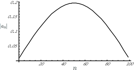
Refer to caption
Figure 2: Distribution of $|a_{n}|$ with odd subscripts for $N=100$ which gives the lower bound in Eq. (164). This figure shows $\frac{1}{C_{\frac{N}{2}}}W_{\frac{n-1}{2}}(x_{\frac{N}{2},1})$ as a function of odd $n$.

For odd $N$, the lower bound can be given by setting the input state and the evolution operator as those analogous to the case of even $N$. The bound is $\frac{1}{2}(1-\cos\frac{2\pi}{N+1})$. The attainability of this bound is also proved by the analogous argument.

Thus, we have shown that

$\displaystyle\min_{(U,|A\rangle)}\max_{\rho_{\mathbf{S}}}D(\mathcal{E}_{U,\left|A\right\rangle}(\rho_{\mathbf{S}}),\mathcal{E}_{X_{\mathbf{S}}}(\rho_{\mathbf{S}}))$ (178)
$\displaystyle=$ $\displaystyle\frac{1}{2}\Big{(}1-\cos\frac{2\pi}{N+2}\Big{)},$

if $N$ is even and

$\displaystyle\min_{(U,|A\rangle)}\max_{\rho_{\mathbf{S}}}D(\mathcal{E}_{U,\left|A\right\rangle}(\rho_{\mathbf{S}}),\mathcal{E}_{X_{\mathbf{S}}}(\rho_{{\mathbf{S}}}))$ (179)
$\displaystyle=$ $\displaystyle\frac{1}{2}\Big{(}1-\cos\frac{2\pi}{N+1}\Big{)}$

if $N$ is odd, where $(U,|A\rangle)$ varies over all the classical complete pure implementation with $N$ qubit ancilla.

For arbitrary $N$, we conclude as a common lower bound

$\displaystyle\min_{(U,|A\rangle)}\max_{\rho_{\mathbf{S}}}D(\mathcal{E}_{U,\left|A\right\rangle}(\rho_{{\mathbf{S}}}),\mathcal{E}_{X_{\mathbf{S}}}(\rho_{\mathbf{S}}))$ (180)
$\displaystyle\geq$ $\displaystyle\frac{1}{2}\Big{(}1-\cos\frac{2\pi}{N+2}\Big{)},$

where $(U,|A\rangle)$ varies over all the classical complete pure implementation with $N$ qubit ancilla.

We have considered the case where the ancilla state is a pure state. The lower bound for the general case is obtained by the previously developed purification argument, and we conclude the following relations. We have

$\displaystyle\max_{\rho_{\mathbf{S}}}D(\mathcal{E}_{U,\rho_{\mathbf{A}}}(\rho_{\mathbf{S}}),\mathcal{E}_{X_{\mathbf{S}}}(\rho_{\mathbf{S}}))$ (181)
$\displaystyle\geq$ $\displaystyle\frac{1}{2}\Big{(}1-\cos\frac{2\pi}{N+\log_{2}\mathrm{rank}{\rho_{\mathbf{A}}}+2}\Big{)},$

for any classically complete implementation $(U,\rho_{\mathbf{A}})$ with $N$ qubit ancilla, and

$\displaystyle\min_{(U,\rho_{\mathbf{A}})}\max_{\rho_{\mathbf{S}}}D(\mathcal{E}_{U,\rho_{\mathbf{A}}}(\rho_{\mathbf{S}}),\mathcal{E}_{X_{\mathbf{S}}}(\rho_{\mathbf{S}}))$ (182)
$\displaystyle\geq$ $\displaystyle\frac{1}{2}\Big{(}1-\cos\frac{\pi}{N+1}\Big{)},$

where $(U,\rho_{\mathbf{A}})$ varies over all the classically complete implementation with $N$ qubit ancilla.

VII Concluding remarks

In this paper, we have studied the precision limit of the quantum NOT gate or the bit flip gate, one of the most basic gates in quantum computation, represented on the single-spin computational qubit by considering the angular momentum conservation law obeyed by the interaction between the computational qubit and the control system supposed to comprise many qubits. Actually, we have considered the effect of the angular momentum conservation law only in the direction same as the computational basis, usually set as the $z$ direction. Then, the conserved quantity and the computational basis are represented by the Pauli $Z$ operator, whereas the quantum NOT gate is represented by the Pauli $X$ operator. Thus, it is expected that this non-commutativity leads to a precision limit of the gate operation.

In the previous method which was used for other gates Ozawa (2002a, 2003c), one finds a way in which the gate under consideration is used as a component of a measuring apparatus, applies the quantitative generalization of the Wigner-Araki-Yanase (WAY) theorem to this measuring apparatus, and obtains the lower bound of error probability. For the Hadamard gate, one finds that it is used to convert the $Z$ measurement to the $X$ measurement, and that $Z$ measurement can be done without error under the conservation law of the $z$ component. Then, one can conclude that the inevitable error of the $X$ measurement, calculated from the quantitative version of the WAY theorem, is yielded from the converter using the Hadamard gate. This and similar arguments cannot be applied to the quantum NOT gate, since the quantum NOT gate does not convert the direction of measurement, but simply flips the measured bit.

In this paper, we have developed a new method for obtaining the inevitable error probability by evaluating the maximum trace distance between the output from the gate realization and the output from the ideal gate. The previous method naturally leads to a lower bound for the infidelity (one minus the squared fidelity). Since the infidelity is dominated by the trace distance, the new method gives a tighter lower bound for the error probability.

The new method is based on a straightforward evaluation of the trace distance of two output states, and enables us to find the precision limit Eq. (72), explicitly described by the input state of the ancilla system. It is thus possible to obtain information on how much an ancilla input has an inherent error probability in itself. The correspondence between the two methods is not easy to elicit, but it is an interesting problem for future studies that would lead to a deeper understanding of precision limits to quantum control systems.

We have also obtained the lower bound (152) expressed by the size of the ancilla system, by minimizing Eq. (72) over the input states of $\mathbf{A}$, using Chebyshev polynomials of the second kind. The lower bound is much tighter than the scaling expected from the previous result based on the WAY theorem. Since the quantitative generalization of the WAY theorem has a close relation to the universal uncertainty principle for measurement and disturbance Ozawa (2003d, c), the previous lower bound for pure conservative implementations is based on the variance of the ancilla state, and scales as $\frac{1}{4N^{2}+4}\approx\frac{1}{4N^{2}}$, whereas the new method revealed the lower bound $\frac{1}{2}(1-\cos\frac{2\pi}{N+4})\approx\frac{\pi^{2}}{N^{2}}$ as a tighter bound. The higer order terms in $\frac{1}{2}(1-\cos\frac{2\pi}{N+4})$ is considered to be meaningful, since the lower bound $\frac{1}{2}(1-\cos\frac{2\pi}{N+2})$ is attained among classically complete pure conservative implementations. Interestingly, the attainability result shows that the best ancilla states to attain the lower bound are not maximum variance states, nor uniformly distributed states, but those states with the distribution determined by the recurrence relation characterized by Chebyshev polynomials.

Although our study has assumed that the ancilla system consists of $N$ qubits for comparison with the previous research, the present method is not restricted to this particular control system, and it can be readily applied to other control systems, such as atom-field systems, where the present method would lead to a lower bound that scales as the inverse of the photon number Gea-Banacloche and Ozawa (2005). Our method will be also expected to contribute to the problem of programmable quantum processors Nielsen and Chuang (1997); Vidal and Cirac (2000); Hillery et al. (2006) and related subjects D’Ariano and Perinotti (2005a, b, c) in future investigations.

Acknowledgements.
The authors thank Hajime Tanaka, Gen Kimura, and Julio Gea-Banacloche for useful discussions and suggestions. This research was partially supported by the SCOPE project of the MIC, the Grant-in-Aid for Scientific Research (B)17340021 of the JSPS, and the CREST project of the JST.

References

  • Shor (1994) P. W. Shor, in Proceedings of the 35th Annual Symposium on Foundations of Computer Science, edited by G. Goldwasser (IEEE Computer Society Press, Los Alamitos, CA, 1994), pp. 124–134.
  • Unruh (1995) W. G. Unruh, Phys. Rev. A 51, 992 (1995).
  • Palma et al. (1996) G. M. Palma, K. A. Suominen, and A. K. Ekert, Proc. R. Soc. Lond. A 452, 567 (1996).
  • Haroche and Raimond (1996) S. Haroche and J.-M. Raimond, Physics Today 49, no. 8, p. 51 (1996).
  • Shor (1995) P. W. Shor, Phys. Rev. A 52, R2493 (1995).
  • Steane (1996) A. M. Steane, Phys. Rev. Lett. 77, 793 (1996).
  • Nielsen and Chuang (2000) M. A. Nielsen and I. L. Chuang, Quantum Computation and Quantum Information (Cambridge University Press, Cambridge, 2000).
  • Ozawa (2003a) M. Ozawa, in Proceedings of the Sixth International Conference on Quantum Communication, Measurement and Computing, edited by J. H. Shappiro and O. Hirota (Rinton Press, Princeton, 2003a), pp. 175–180.
  • Barnes and Warren (1999) J. P. Barnes and W. S. Warren, Phys. Rev. A 60, 4363 (1999).
  • Gea-Banacloche (2002) J. Gea-Banacloche, Phys. Rev. A 65, 022308 (2002).
  • van Enk and Kimble (2002) S. J. van Enk and H. J. Kimble, Quantum Inf. Comput. 2, 1 (2002).
  • Ozawa (2002a) M. Ozawa, Phys. Rev. Lett. 89, 057902 (2002a).
  • Wigner (1952) E. P. Wigner, Z. Phys. 133, 101 (1952).
  • Araki and Yanase (1960) H. Araki and M. M. Yanase, Phys. Rev. 120, 622 (1960).
  • Ozawa (2003b) M. Ozawa, Phys. Rev. Lett. 91, 089802 (2003b).
  • Lidar (2003) D. A. Lidar, Phys. Rev. Lett. 91, 089801 (2003).
  • Kawano and Ozawa (2006) Y. Kawano and M. Ozawa, Phys. Rev. A 73, 012339 (2006).
  • Ozawa (2002b) M. Ozawa, Phys. Rev. Lett. 88, 050402 (2002b).
  • Ozawa (2003c) M. Ozawa, Int. J. Quant. Inf. 1, 569 (2003c).
  • Ozawa (2003d) M. Ozawa, Phys. Rev. A 67, 042105 (2003d).
  • Ozawa (2003e) M. Ozawa, Phys. Lett. A 318, 21 (2003e).
  • Ozawa (2004) M. Ozawa, Ann. Phys. (N.Y.) 311, 350 (2004).
  • Gea-Banacloche and Ozawa (2005) J. Gea-Banacloche and M. Ozawa, J. Opt. B: Quantum Semiclass. Opt. 7, S326 (2005).
  • Itano (2003) W. M. Itano, Phys. Rev. A 68, 046301 (2003).
  • Silberfarb and Deutsch (2004) A. Silberfarb and I. H. Deutsch, Phys. Rev. A 69, 042308 (2004).
  • van Enk and Kimble (2003) S. J. van Enk and H. J. Kimble, Phys. Rev. A 68, 046302 (2003).
  • Gea-Banacloche (2003) J. Gea-Banacloche, Phys. Rev. A 68, 046303 (2003).
  • Nielsen and Chuang (1997) M. A. Nielsen and I. L. Chuang, Phys. Rev. Lett. 79, 321 (1997).
  • Vidal and Cirac (2000) C. Vidal and J. I. Cirac, Storage of quantum dynamics in quantum states: a quasi-perfect programmable quantum gate (2000), e-print quant-ph/0012067.
  • Hillery et al. (2006) M. Hillery, M. Ziman, and V. Bužek, Phys. Rev. A 73, 022345 (2006).
  • D’Ariano and Perinotti (2005a) G. M. D’Ariano and P. Perinotti, Phys. Rev. Lett. 94, 090401 (2005a).
  • D’Ariano and Perinotti (2005b) G. M. D’Ariano and P. Perinotti, On the most efficient unitary transformation for programming quantum channels (2005b), e-print quant-ph/0509183.
  • D’Ariano and Perinotti (2005c) G. M. D’Ariano and P. Perinotti, Programmable quantum channels and measurements (2005c), e-print quant-ph/0510033.
  • Paulsen (1986) V. I. Paulsen, Completely bounded maps and dilations, Pitman Resarch Notes in Math. 146 (Longman, New York, 1986).
  • Belavkin et al. (2005) V. P. Belavkin, G. M. D’Ariano, and M. Raginsky, J. Math. Phys. 46, 062106 (2005).
  • Hotta et al. (2005) M. Hotta, T. Karasawa, and M. Ozawa, Phys. Rev. A 72, 052334 (2005).
  • Szego (1967) G. Szego, Orthogonal Polynomials (American Mathematical Society, Providence, R.I., 1967).
  • Chihara (1978) T. S. Chihara, An Introduction to Orthogonal Polynomials (Gordon and Breach, New York, 1978).