A dynamical analysis of the 14 Her planetary system

Abstract

Precision radial velocity (RV) measurements of the Sun-like dwarf 14 Herculis published by Naef et. al (2004), Butler et. al (2006) and Wittenmyer et al (2007) reveal a Jovian planet in a 1760 day orbit and a trend indicating the second distant object. On the grounds of dynamical considerations, we test a hypothesis that the trend can be explained by the presence of an additional giant planet. We derive dynamical limits to the orbital parameters of the putative outer Jovian companion in an orbit within $\sim 13$ AU. In this case, the mutual interactions between the Jovian planets are important for the long-term stability of the system. The best self-consistent and stable Newtonian fit to an edge-on configuration of Jovian planets has the outer planet in 9 AU orbit with a moderate eccentricity $\sim 0.2$ and confined to a zone spanned by the low-order mean motion resonances 5:1 and 6:1. This solution lies in a shallow minimum of ${(\chi^{2}_{\nu})^{1/2}}$ and persists over a wide range of the system inclination. Other stable configurations within $1\sigma$ confidence interval of the best fit are possible for the semi-major axis of the outer planet in the range of (6,13) AU and the eccentricity in the range of (0,0.3). The orbital inclination cannot yet be determined but when it decreases, both planetary masses approach $\sim 10\mbox{m}_{{\mbox{\scriptsize J}}}$ and for $i\sim 30^{{\rm o}}$ the hierarchy of the masses is reversed.

1 Introduction

An extrasolar planet around 14 Herculis discovered by the Geneva planet search team was announced in a conference talk (1998). The star was also monitored by other planet-hunting teams. The Jovian companion in $\sim 1700$ days orbit was next confirmed by Butler et al. (2003). In their new paper, the discovery team (Naef et al., 2004) published 119 observations revealing a linear RV trend of $\sim 3.6$ m/s per year. The single planet Keplerian solution to these measurements yielded an abnormally large rms of about $14$ m/s. Even if the drift was accounted for, the rms of the single planet+drift model was $\sim 11.3$ m/s, significantly larger than the mean observational uncertainty $\langle\sigma_{{\mbox{\scriptsize m}}}\rangle\sim 7.2$ m/s quoted in that paper.

Following the hypothesis that the linear trend in the RV data may indicate other, more distant bodies, in Goździewski et al. (2006), we merged these measurements with accurate, 35 observations (the mean of $\sigma_{{\mbox{\scriptsize m}}}\sim 3.1$ m/s) by Butler et al. (2003), spanning the middle part of the combined observational window. We reanalyzed the full data set of 154 measurements, covering about $3400$ days, $\sim 2P_{{\mbox{\scriptsize b}}}$. Using our GAMP method (Goździewski et al., 2003), i.e., the optimization incorporating stability constraints into the fitting algorithm, we searched for stable configurations of putative two-planet systems which are consistent with the RV data. This search revealed many stable solutions, in particular two distinct and equally good best fits with $a_{{\mbox{\scriptsize c}}}\sim 5.8$ AU and $a_{{\mbox{\scriptsize c}}}\sim 9$ AU. They were localized in the proximity of low-order mean motion resonances (MMRs), 3:1 MMR (14 Her^a) and 6:1 MMR (14 Her^b). Apparently, the companions would be well separated, but the system would still be active dynamically. The dynamical maps computed in the neighborhood of the selected fits revealed a complex structure of the phase space. We found a clear relation of chaotic motions to strongly unstable, self-disrupting configurations on a short time-scale of $10^{4}$ periods of the outermost planet.

After the upgrade of HIRES spectrograph and improvements to the data pipeline, Butler et al. (2006) have re-analyzed their spectra and published a revised set of 50 observations of 14 Her. Their mean accuracy $\sim 2.4$ m/s is already very good. Yet, towards the end of the observational window, single data points have formal errors as small as 1 m/s. Recently, Wittenmyer et al. (2007) have also published 35 additional and independent precision measurements made at the McDonald Observatory. They have a mean accuracy of 7.5 m/s. The full publicly available data set is now comprised of 203 observations spanning 4463.2 days and still does support the presence of a second planetary object. The single-planet solution has an rms $\sim 13$ m/s, and shows a few meter per second excess over the mean $\sigma_{{\mbox{\scriptsize m}}}\sim 6$ m/s, added in quadrature to the stellar jitter $\sim 3.5$ m/s (Butler et al., 2006). Using the Keplerian model of the RV, Wittenmyer et al. (2007) have found the best-fit solution in the vicinity of the 4:1 mean motion resonance (MMR). However, having in mind the results of our earlier dynamical analysis (Goździewski et al., 2006), we can suspect that the kinematic model is not adequate to properly interpret the RV observations.

In this paper, we re-analyse the updated high-precision RV data to study and extend the kinematic model by Wittenmyer et al. (2007). We also revise and correct the conclusions from our previous paper (Goździewski et al., 2006) that were derived on the basis of a smaller and less precise RV data set. The goal of our work is to derive dynamical characteristics of the putative planetary system and to place limits on its orbital parameters. Assuming a putative configuration close to the 4:1 MMR, the outermost orbital period would be $\sim 18$–$20$ yr. Hence, the currently available data would cover only a part of this period and a full characterization of the orbits would still require many years of observations. One cannot expect that in such a case the orbits can be well determined. Nevertheless, we show in this work, that the modeling of the RV data when merged with a dynamical analysis and mapping of the phase space of initial conditions with fast-indicators enable us to derive meaningful limits to the orbital parameters. Such an extensive dynamical study of this systems has not yet been done.

In order to take into account the RV variability induced by the stellar activity, the internal errors of the RV measurements are rescaled by the jitter added in quadrature: $\sigma^{2}=\sigma_{{\mbox{\scriptsize m}}}^{2}+\sigma_{{\mbox{\scriptsize j}}}^{2},$ where $\sigma_{{\mbox{\scriptsize m}}}$ and $\sigma_{{\mbox{\scriptsize j}}}$ are the mean of the internal errors and the adopted estimate of the stellar jitter. The 14 Herculis is a quiet star with $\log R^{\prime}_{{\mbox{\scriptsize HK}}}=-5.07$ (Naef et al., 2004) thus it is reasonable to keep the safe estimate of $\sigma{{\mbox{\scriptsize j}}}=3.5$ m/s (Butler et al., 2006). The mass of the parent star varies by $\sim 10\%$ in different publications. In this work, we adopt the canonical mass $1\mbox{M}_{\sun}$, although we also did some calculations for the mass of $0.9\mbox{M}_{\sun}$ and $1.1\mbox{M}_{\sun}$.

                   

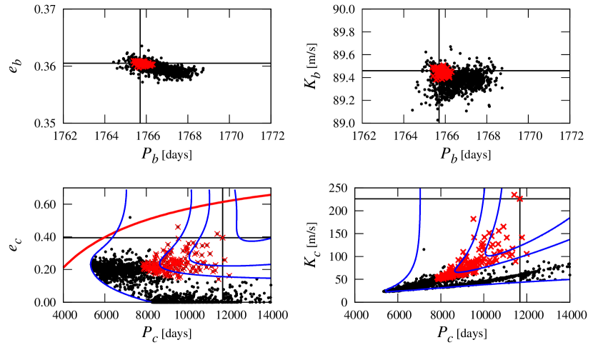
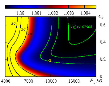
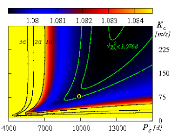
Figure 1: The best fit solutions to the two-planet model of the RV data of 14 Her in the ($P,e$)- and ($P,K$)-plane. In the search, a distant companion to the known Jovian planet in $\sim 1760$ days orbit is assumed. Upper plots are for the inner planet, middle plots are for the outer one. The best-fit found with the hybrid code in the range of moderate orbital periods of the outer planet, with ${(\chi^{2}_{\nu})^{1/2}}\sim 1.085$, is marked with intersecting lines. Its elements, in terms of the parameter tuples of Eq.1, $(K\mbox{[m/s]},P\mbox{[days]},e,\omega\mbox{[deg]},T_{{\mbox{\scriptsize p}}}-T_{0}\mbox{[days]})$, are (89.460, 1765.743, 0.360, 22.108, 1375.03) for the inner and (226.2263, 11675.333, 0.395, 182.006, 6115.352 ) for the outer planet, respectively, with the velocity offsets ($V_{{\mbox{\scriptsize N2004}}},V_{{\mbox{\scriptsize B2006}}},V_{{\mbox{\scriptsize W2007}}}$) $=$ (-129.105, -132.345, -108.384) m/s for the data in (Naef et al., 2004), (Butler et al., 2006) and (Wittenmyer et al., 2007), respectively; the epoch $T_{0}=$ JD2,450,000. Dots are for $1\sigma$ solutions with ${(\chi^{2}_{\nu})^{1/2}}\in[1.0848,1.090)$ and an rms $\sim 8.17$ m/s, red crosses are for the the best fit solutions with ${(\chi^{2}_{\nu})^{1/2}}\sim 1.0848$. The red curve in ($P_{{\mbox{\scriptsize c}}},e_{{\mbox{\scriptsize c}}}$)-plane marks an approximate collision line of the orbits determined from $a_{{\mbox{\scriptsize b}}}(1+e_{{\mbox{\scriptsize b}}})=a_{{\mbox{\scriptsize c}}}(1-e_{{\mbox{\scriptsize c}}})$, with $a_{{\mbox{\scriptsize b}}},e_{{\mbox{\scriptsize b}}}$ fixed at their best-fit values. Bottom panels are for the scans of ${(\chi^{2}_{\nu})^{1/2}}$ at the selected parameter planes. Contours (also shown in the upper panels, for a reference) mark the limits of ${(\chi^{2}_{\nu})^{1/2}}$ corresponding to $1\sigma,2\sigma$ and $3\sigma$ of the best fit solution. Circle mark the position of the best $N$-body solution (see Sect. 4). See the text for remaining details.

2 Modeling the RV data – an overview

The standard formulae by Smart (1949) are commonly used to model the RV signal. Each planet in the system contributes to the reflex motion of the star at time $t$ with:

$$V_{{\mbox{\scriptsize r}}}(t)=K[\cos(\omega+\nu(t))+e\cos\omega]+V_{0},$$ (1)

where $K$ is the semi-amplitude, $\omega$ is the argument of pericenter, $\nu(t)$ is the true anomaly (involving implicit dependence on the orbital period $P$ and time of periastron passage $T_{{\mbox{\scriptsize p}}}$), $e$ is the eccentricity, $V_{0}$ is the velocity offset. We interpret the primary model parameters $(K,P,e,\omega,T_{{\mbox{\scriptsize p}}})$ in terms of the Keplerian elements and minimal masses related to Jacobi coordinates (Lee & Peale, 2003; Goździewski et al., 2003).

In our previous works, we tested and optimized different tools used to explore the multi-parameter space of $\chi^{2}$. In the case when $\chi^{2}$ has many local extrema, we found that the hybrid optimization provides particularly good results (Goździewski & Konacki, 2004; Goździewski & Migaszewski, 2006). A run of our code starts the genetic algorithm (GA, Charbonneau, 1995) that basically has a global nature and requires only the $\chi^{2}$ function and rough parameter ranges. GA easily permits for a constrained optimization within prescribed parameter bounds or for a penalty term to $\chi^{2}$ (Goździewski et al., 2006). Because the best fits found with GAs are not very accurate in terms of $\chi^{2}$, we refine a number of “fittest individuals” in the final “population” with a relatively fast local method like the simplex of Melder and Nead (Press et al., 1992). The use of simplex algorithm is a matter of choice and in principle we could use other fast local methods. However, a code using non-gradient methods works with the minimal requirements for the user-supplied information, i.e., the model function, usually equal to $\chi^{2}$ [its inverse $1/\chi^{2}$ is the fitness function required by GAs]. The repeated runs of the hybrid code provide an ensemble of the best-fits that helps us to detect local minima of $\chi^{2}$, even if they are distant in the parameter space. We can also obtain reliable approximation to the errors of the best-fit parameters (Bevington & Robinson, 2003) within the $1\sigma$, $2\sigma$ and $3\sigma$ confidence levels of $\chi^{2}$ at selected 2-dim parameter planes, as corresponding to appropriate increments of $\chi^{2}$. The hybrid approach will be called the algorithm I from hereafter.

However, in this paper we deal with a problem of only a partial coverage of the longest orbital period by the data. In such a case $\chi^{2}$ does not have a well defined minimum or the space of acceptable solutions is very “flat” so the confidence levels may cover large ranges of the parameters. In such a case, to illustrate the shape of $\chi^{2}$ in the selected 2-dimensional parameter planes, we use a complementary approach that relies on systematic scanning of the parameter space with the fast Levenberg-Marquardt (L-M) algorithm (Press et al., 1992). Usually, as the parameter plane for representing such scans, we choose the semimajor-axis—eccentricity $(a,e)$ plane of the outermost planet. We fix $(a,e)$ and then search for the best fit, with the initial conditions selected randomly (but within reasonably wide parameter bounds). Then the L-M scheme ensures a rapid convergence. This approach is called the algorithm II from hereafter. In fact, we already used it in Goździewski et al. (2003). The method is CPU-time consuming and may be effectively applied in low-dimensional problems but in reward it can provide a clear and global picture of the parameter space.

Moreover, the RV measurements can be polluted by many sources of error, like complex systematic instrumental effects, short time-series of the observations, irregular sampling due to observing conditions, and stellar noise. The problem is even more complex when we deal with models of resonant or strongly interacting planetary systems. It is well known that the kinematic model of the RV is not adequate to describe the observations in such instances. Instead, the self-consistent $N$-body Newtonian model should be applied (Rivera & Lissauer, 2001; Laughlin & Chambers, 2001). (Note that the hybrid optimization can be used to explore the parameter space for both models). Still, the best-fit solutions may be related (and often do) to unrealistic quickly disrupting configurations (Ferraz-Mello et al., 2005; Lee et al., 2006; Goździewski et al., 2006). In such a case one should explore the dynamical stability of the planetary system in a neighborhood of the best-fit configuration. One can do that with the help of direct numerical integrations or by resolving the dynamical character of orbits in terms of the maximal Lyapunov exponent or the diffusion of fundamental frequencies. Hence, the most general way of modeling the RV data should involve an elimination of unstable (for instance, strongly chaotic) solutions during the fitting procedure. We described such an approach (called GAMP) in our previous works. In particular, we made attempts to analyze the old data set of 14 Her as well as other stars hosting multiple planet systems (Goździewski et al., 2006).

3 Keplerian fits

In order to compare our fits with the results of Wittenmyer et al. (2007), we carried out the hybrid search for the two-planet edge-on configuration. In the experiment, we limited the orbital periods to the range of $[1000,14000]$ days and the eccentricities to the range of $[0,0.9]$. The choice of the upper limit of orbital periods followed the conclusions of Wittenmyer et al. (2007). According to the results of adaptive-optics imaging by Luhman & Jayawardhana (2002) and Patience et al. (2002), the parent star has no stellar companion beyond $9$ — $12$ AU, so we try to verify the hypothesis about a short-period, low-mass companion 14 Her c up to that distance. The RV offsets are different for each of the three instruments and are included as free parameters in the model together with the tuples of $(K,P,e,\omega,T_{{\mbox{\scriptsize p}}})$ for each companion. Note that we calculate the RV offset $V_{{\mbox{\scriptsize N2004}}}$ with respect to the simple mean of all RV measurements from the set published by Naef et al. (2004).

The results of the hybrid search (algorithm I) are illustrated in upper panels Fig. 1 (note that before plotting, the fits are sorted with respect to the smaller semi-major axis). The best-fit found with this method has ${(\chi^{2}_{\nu})^{1/2}}\simeq 1.085$ and an rms $\simeq 8.17$ m/s. Its parameters are given in the caption to Fig. 1. Clearly, there is no isolated best-fit solution but rather a huge number of acceptable fits. The ratio of the orbital periods within $1\sigma$ confidence interval of the best fit may be as low as $\sim 3$. The orbital period in the best fit is $\sim 12000$ days and $P_{{\mbox{\scriptsize c}}}/P_{{\mbox{\scriptsize b}}}\sim 7$. This is roughly consistent with the work of Wittenmyer et al. (2007) who quote the best-fit configuration close to the 4:1 MMR and with a similar rms $8.17$ m/s. Yet the fits are not constrained with respect to $P_{{\mbox{\scriptsize c}}}$. Many values between $[5000,14000]$ days are equally good in terms of $1\sigma$ confidence interval of the best-fit solution. Moreover, it means that the system may be confined to a zone spanned by many low-order mean motion resonances of varying width in the $(P_{{\mbox{\scriptsize c}}},e_{{\mbox{\scriptsize c}}})$-plane. In such cases, the mutual interactions between the planets are important for the long-term stability.

In order to illustrate the shape of ${(\chi^{2}_{\nu})^{1/2}}$ in more detail, we also applied the algorithm II for the systematic scanning of that function in selected parameter planes (see lower panels in Fig. 1). This has lead to even better statistics of the best fits and a very clear illustration of the ${(\chi^{2}_{\nu})^{1/2}}$-surface. The panels reveal that ${(\chi^{2}_{\nu})^{1/2}}$ of 2-Kepler model has no minimum in the examined ranges of the outermost periods, $P_{{\mbox{\scriptsize c}}}<14,000$ days.

Along a wide valley, the best fits with an increasing $P_{{\mbox{\scriptsize c}}}$ have also rapidly increasing $e_{{\mbox{\scriptsize c}}}$. For $P_{{\mbox{\scriptsize c}}}\sim 14,000$ days, they reach the collision zone of the orbits. In this strongly chaotic region a number of MMRs of the type $p:1$ with $p>7$ overlap. It justifies a-posteriori our choice of the search limit $P_{{\mbox{\scriptsize c}}}\sim 14,000$ days. Note, that the two searches are in an excellent accord that is illustrated with the ${(\chi^{2}_{\nu})^{1/2}}$ smooth contour levels overlayed on the results of the hybrid search. In that case, the scanning of parameter space helps to understand the shape of ${(\chi^{2}_{\nu})^{1/2}}$ in detail.

The $1\sigma$ scatter of solutions around the best-fit (Fig. 1) provides realistic error estimates. Although the parameters of the inner planet are very well fixed, the elements of the outer Jovian planet have much larger formal errors. The kinematic fits do not provide an upper bound to the semi-major axis of the outer planet. Both methods reveal exactly the same parameters of the inner companion (see Fig. 1). Obviously, certain discrepancy between the outcomes of algorithm I and algorithm II is related to a “flat” shape of ${(\chi^{2}_{\nu})^{1/2}}$ in the $(a_{{\mbox{\scriptsize c}}},e_{{\mbox{\scriptsize c}}})$-plane and to a worse efficiency of simplex in detecting shallow minima compared to the gradient-like L-M algorithm. When ${(\chi^{2}_{\nu})^{1/2}}$ does not have a well localized minimum, it is very difficult to resolve its behaviour with any non-gradient method.

4 Self-consistent Newtonian fits

In order to compare the outcome of kinematic modeling with the self-consistent $N$-body one, at first, we transformed the ensemble of Keplerian fits to astro-centric osculating elements (Lee & Peale, 2003; Goździewski et al., 2003). These fits became the initial conditions for the L-M algorithm employing the $N$-body model of the RV. In this experiment, the mass of the star was $M_{\star}=1~{}M_{\sun}$. Curiously, we found that the procedure often converged to the two best-fits, both having similar ${(\chi^{2}_{\nu})^{1/2}}\sim 1.083$, an rms $\sim 8.15$ m/s, and $a_{{\mbox{\scriptsize c}}}\sim 7.8$ AU and $a_{{\mbox{\scriptsize c}}}\sim 8.4$ AU, respectively. To shed some light on the orbital stability of these solutions, we computed the dynamical maps in the neighborhood of the best-fits in terms of the Spectral Number ($\log SN$, Michtchenko & Ferraz-Mello, 2001). We chose $a_{{\mbox{\scriptsize c}}}$ and $e_{{\mbox{\scriptsize c}}}$ as the map coordinates, keeping other orbital parameters at their nominal values. The results are shown in Fig. 2. The left panel is for the unstable fit located in the separatrix of the 5:1 MMR. The right panel is for the stable solution in the center of 9:2 MMR. These dynamical maps prove that the mutual interactions between planets are significant — even small changes of initial parameters modify the shapes of low-order MMRs which overlap already for $e_{{\mbox{\scriptsize c}}}\sim 0.2-0.3$. Besides, the chaotic motions are related to strongly unstable configurations (see also Fig. 3, 4).

         

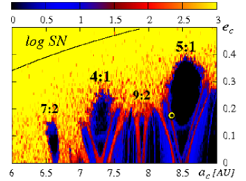
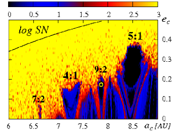
Figure 2: The dynamical maps in terms of the Spectral Number ($\log SN$) in the $(a_{{\mbox{\scriptsize c}}},e_{{\mbox{\scriptsize c}}})$-plane for the two-planet Newtonian models of the 14 Her system. Colors used in the $\log SN$ map classify the orbits — black indicates quasi-periodic regular configurations while yellow strongly chaotic ones. The maps are computed for the following osculating elements of the Jovian planets at the epoch of the first observation $t_{0}$, in terms of tuples $(m~{}[m_{{\mbox{\scriptsize J}}}],a~{}[\mbox{AU}],e,\omega~{}[\mbox{deg}],{\cal M}(t_{0})~{}[\mbox{deg}])$: the left panel is for (4.975, 2.864, 0.359, 22.281, 330.365) of the inner planet, and (5.618, 8.343, 0.174, 188.543, 72.091) of the outer planet, respectively; the right panel is for (4.974, 2.863, 0.359, 22.310, 330.314) of the inner planet, and (4.558, 7.863, 0.173, 187.674, 64.417) of the outer planet, respectively. The large circles mark the parameters of the best fits. The thin line marks the collision curve for planets b and c, as determined by $a_{{\mbox{\scriptsize b}}}(1+e_{{\mbox{\scriptsize b}}})=a_{{\mbox{\scriptsize c}}}(1-e_{{\mbox{\scriptsize c}}})$. The low-order MMRs of the planets b and c are labeled. The integrations are conducted over $\sim 10^{4}P_{{\mbox{\scriptsize c}}}$. The resolution is $500\times 120$ data points.

As in the case of the Keplerian model, to resolve the topology of ${(\chi^{2}_{\nu})^{1/2}}$ in detail, we performed similar searches for the best-fit configurations using the $N$-body model of the RV. Again, the results of the hybrid algorithm are consistent with the algorithm II. However, to conserve space, we only show the ${(\chi^{2}_{\nu})^{1/2}}$-maps obtained by scanning the ($a_{{\mbox{\scriptsize c}}},e_{{\mbox{\scriptsize c}}}$)-plane. The results are illustrated in the left column panels of Fig. 3.

These scans are computed for three different and fixed values of the inclination of the putative orbital plane of the system, $i=90^{\circ}$, $60^{\circ}$ and $30^{\circ}$, respectively. In the maps, we mark a few contour levels of ${(\chi^{2}_{\nu})^{1/2}}$ that correspond to $1\sigma,2\sigma$ and $3\sigma$-levels of the best fit solution denoted with a circle in every panel.

Overall, the topology of ${(\chi^{2}_{\nu})^{1/2}}$ does change, nevertheless qualitatively certain features are common. Contrary to the Keplerian case, we can detect a shallow minimum of ${(\chi^{2}_{\nu})^{1/2}}$ close to (9 AU,0.2) and a hint of another minimum localized far over the collision line. The white thick lines on the panels mark mass limits of $m_{{\mbox{\scriptsize c}}}$. Clearly, for $a_{{\mbox{\scriptsize c}}}>9$ AU and for moderate eccentricity, $m_{{\mbox{\scriptsize c}}}$ approaches the brown-dwarf mass limit and substellar mass 80 $m_{{\mbox{\scriptsize J}}}$ for $\sim 12$ AU. Thus a brown-dwarf could exist in the system beyond $10$-$11$ AU depending on the inclination and eccentricity — and the fits preclude a low-mass planetary object over the 14 $m_{{\mbox{\scriptsize J}}}$ level.

Note, that the best-fit for the nominal edge-on configuration with $i=90^{\circ}$ turns out to be unstable but its parameters are very close to a stable solution given in Table 1; its synthetic curve is illustrated in Fig. 5.

To characterize the stability of the best-fit solutions, we computed their MEGNO fast indicator (Cincotta & Simó, 2000), $\langle Y\rangle$, (i.e., an approximation of the maximal Lyapunov exponent) up to $\sim 2\times 10^{5}~{}P_{{\mbox{\scriptsize c}}}$ using a fast and accurate symplectic algorithm (Goździewski et al., 2005). The total integration time $3$-$4$ Myr is long enough to detect even weak unstable MMRs.

The best-fits that passed the MEGNO test (i.e. that are regular over the integration time) are marked with black dots in the right panels of Fig. 3. For a reference, the $\sigma$-levels of ${(\chi^{2}_{\nu})^{1/2}}$ from the respective left-panels are marked in these plots as well. The red curves are for the collision line of the orbits computed for well constrained and fixed parameters of the inner planet. Overall, the stable solutions reveal the structure of the MMRs that we have already seen in the dynamical maps computed for fixed orbital parameters (see Fig. 2). The semi-major axis of the outer planet cannot be yet constrained well and may vary between $6$ AU and (at least) 13 AU. Moreover there is a rather evident although irregular border $e_{{\mbox{\scriptsize c}}}\sim 0.3$ of all solutions, up to $3\sigma$. Besides, we found that in the relevant range of $a_{{\mbox{\scriptsize c}}}$, the mean longitude $\lambda_{{\mbox{\scriptsize c}}}=\varpi_{{\mbox{\scriptsize c}}}+{\cal M}_{{\mbox{\scriptsize c}}}\sim(200^{\circ},300^{\circ})$ within the $1\sigma$ interval of the best fit, increasing along quasi-parabolic curve as the function of $a_{{\mbox{\scriptsize c}}}$. Simultaneously, $\lambda_{{\mbox{\scriptsize b}}}\sim 352.6^{\circ}\pm 1.5^{\circ}$. From the dynamical point of view, this provides significant limits on the relative mean phases of the planets.

The results for two-planet 14 Her system in Goździewski et al. (2006) are basically in accord with the present work although not all conclusions are confirmed. The two isolated minima of ${(\chi^{2}_{\nu})^{1/2}}$ found in that paper can be identified in this work too. In particular it concerns the narrow 3:1 MMR island. The second solution close to the 6:1 MMR has also been found close to the present best fit solution. Nevertheless, the more extensive current search reveals many other stable solutions between 3:1 and 9:1 MMRs equally good in terms of $1\sigma$. Thus the results of our previous work are not wrong in general but rather incomplete — it appears that the search performed was not exhaustive enough to find all acceptable solutions. Still, some of the unstable solutions can be modified in order to obtain stable fits, possibly with slightly increased ${(\chi^{2}_{\nu})^{1/2}}$. For instance, the stability maps in Fig. 3 seem to rule out the 4:1 MMR in the system what may be related to specific orbital phases. After an appropriate change of these phases [still keeping ${(\chi^{2}_{\nu})^{1/2}}$ at acceptable level] we could find also stable solutions close to the 4:1 MMR. In order to do this in a self-consistent manner, a GAMP-like method would be necessary. However, as we have shown, ${(\chi^{2}_{\nu})^{1/2}}$ is very flat in the interesting range of orbital parameters. Then, the extensive enough GAMP search would require a very significant amount of CPU time, so we decided not to do it.

Table 1: Astrocentric, osculating Keplerian parameters of the edge-on, best-fit, self-consistent configuration of 14 Her system at the epoch of the first observation, $t_{0}=$ JD 2459464.5956. The mass of the parent star is 1.0 $M_{\sun}$. See the text and Fig. 3 for the error estimates. The RV offsets $V_{{\mbox{\scriptsize N2004}}}$, $V_{{\mbox{\scriptsize B2006}}}$, and $V_{{\mbox{\scriptsize W2007}}}$ label the data sets published in (Naef et al., 2004; Butler et al., 2006; Wittenmyer et al., 2007), respectively; the offset of $V_{{\mbox{\scriptsize N2004}}}$ is given with respect to the mean of RV in (Naef et al., 2004). ${\cal M}$ denotes the mean anomaly at the epoch $t_{0}$.

parameter	planet b	planet c
$m$ [m${}_{{\mbox{\scriptsize J}}}$]	4.975	7.679
$a$ [AU]	2.864	9.037
$P$ [days]	1766	9886
$e$	0.359	0.184
$\omega$ [deg]	22.230	189.076
${\cal M}(T_{0})$ [deg]	330.421	81.976
$V_{{\mbox{\scriptsize N2004}}}$ [m s-1]	-52.049
$V_{{\mbox{\scriptsize B2006}}}$ [m s-1]	-55.290
$V_{{\mbox{\scriptsize W2007}}}$ [m s-1]	-31.368
${(\chi^{2}_{\nu})^{1/2}}$	1.0824
rms [m s-1]	8.15

Finally, using the algorithm II, we try to resolve the topology of ${(\chi^{2}_{\nu})^{1/2}}$ with respect to a varying mass of the star and inclination of the system (both can be free parameters in the model) but assuming that the system remains coplanar. Adopting the uncertainty of the 14 Her mass $\sim 10\%$ (Butler et al., 2006), we choose $0.9\mbox{M}_{\sun},1.0\mbox{M}_{\sun},1.1\mbox{M}_{\sun}$, and inclinations of orbital plane as $90^{\circ}$ (the edge-on system), $60^{\circ},45^{\circ},30^{\circ}$. Apparently, the distributions of the best-fits are similar for all ($\mbox{M}_{\star},i$)-pairs. Their quality in terms of ${(\chi^{2}_{\nu})^{1/2}}$ is comparable.

The significant differences between the best-fit configurations are related to their stability. To address this issue, we calculated the dynamical maps for the best fits derived for the nominal mass of the parent star ($1~{}\mbox{M}_{\sun}$) and inclinations $90^{\circ}$ (the edge-on system, Table 1), $60^{\circ}$, and $30^{\circ}$ (see Fig. 4,6). The $\log SN$ maps are accompanied by the maximal eccentricity maps, $\max e_{{\mbox{\scriptsize c}}}$, i.e., the eccentricity attained by the orbit during the total integration time. The $\max e$ indicator makes it possible to resolve a link between formally chaotic character of orbits with their physical, short-term instability. In the regions where chaos is strong, the maximal eccentricity grows quickly to 1, implying ejections or collisions between the planets or with the star.

The nominal system lies in a stable zone between 5:1 and 6:1 MMRs (see Fig. 4). However, for the inclination of $\sim 60^{\circ}$, the best fit configuration appears locked in the 5:1 MMR. Overall, the phase space does not change significantly compared to the edge-on system (Fig. 4, also Fig. 2). For the inclination of $30^{\circ}$, the stable zone shrinks due to strong interactions caused by large masses of the planets $\sim 10\mbox{m}_{{\mbox{\scriptsize J}}}$ (see caption to Fig. 6). Moreover, the masses are not simply scaled by factor $1/\sin i$, as one would expect, assuming the kinematic model of the RV. Instead, already for $i\sim 30^{\circ}$, the mass hierarchy is reversed – the inner planet becomes more massive than the outer one. It is yet another argument against the kinematic model of the RV data. The best-fits derived for small inclinations are confined to a strongly chaotic zone. Comparing the dynamical map for $i\sim 30^{{\rm o}}$ with Fig. 4, we conclude that is unlikely to find stable systems close to the formal best fit with $a_{{\mbox{\scriptsize c}}}\sim 9$ AU unless they are trapped in 5:1 MMR. The resonance island can be seen at the edge of the bottom panels in Fig. 6. The planetary masses close to the minimum of ${(\chi^{2}_{\nu})^{1/2}}$ remain smaller from the brown-dwarf limit even for relatively small inclinations of the orbital plane.

              

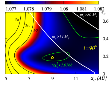
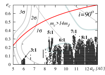
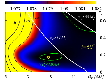
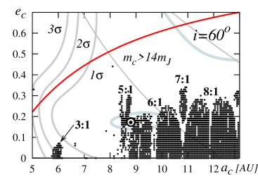
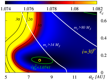
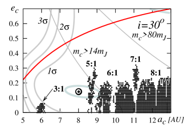
Figure 3: The panels in the left column are for the Newtonian best-fit model with varying fixed inclination of the coplanar system $i$ and illustrated as projections onto the $(a{{\mbox{\scriptsize c}}},e_{{\mbox{\scriptsize c}}})$-plane of initial osculating elements at the epoch of the first observation. In each panel, the best fit is marked with a circle. The quality of the fits within formal $1\sigma,2\sigma$ and $3\sigma$ confidence interval of the best fit, in terms of their ${(\chi^{2}_{\nu})^{1/2}}$ is marked with contours and labeled in subsequent panels. White thick lines corresponds to mass levels of a brown-dwarf and sub-stellar companion, respectively. These solutions are derived with algorithm II. The panels in the right column are for the stability analysis of the best-fit configurations. See the text for more explanation.

                   

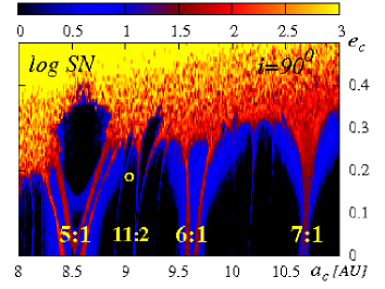
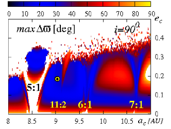
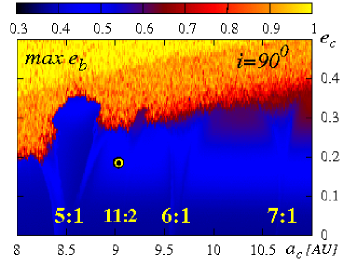
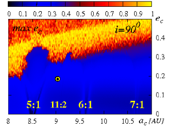
Figure 4: The dynamical maps in the $(a_{{\mbox{\scriptsize c}}},e_{{\mbox{\scriptsize c}}})$-plane in terms of the Spectral Number ($\log SN$, the top-left panel), $\max\Delta\varpi$ relative to the libration mode $180^{\circ}$ (the top-right panel) and $\max e_{{\mbox{\scriptsize b,c}}}$ (the bottom panels) for the two-planet edge-on coplanar Newtonian best-fit model of the 14 Her system (Table 1). Colors used in the $\log SN$ map classify the orbits — black indicates quasi-periodic regular configurations while yellow strongly chaotic ones. The large crossed circles mark the parameters of the fit. The low-order MMRs of the planets b and c are labeled. The integrations are conducted over $\sim 10^{4}P_{{\mbox{\scriptsize c}}}$. The resolution is $500\times 120$ data points.

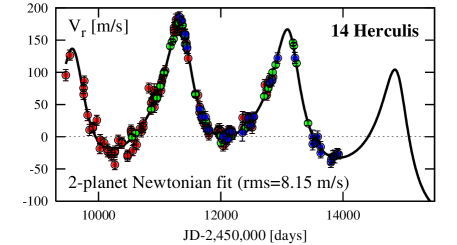
Figure 5: Synthetic RV curve of the self-consistent best fit to the two-planet model. The osculating elements at the epoch of the first observation are given in Table 1. This fit yields ${(\chi^{2}_{\nu})^{1/2}}\sim 1.082$ and an rms $\sim 8.15$ m/s. Observations from Naef et al. (2004), Butler et al. (2006) and Wittenmyer et al. (2007) are marked with red, blue and green circles, accordingly.

                   

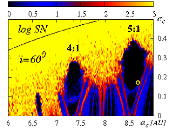
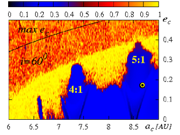
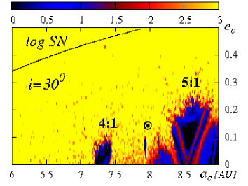
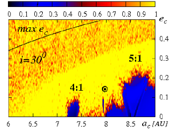
Figure 6: The dynamical maps in the $(a_{{\mbox{\scriptsize c}}},e_{{\mbox{\scriptsize c}}})$-plane in terms of the Spectral Number ($\log SN$, the left panels), and $\max e_{{\mbox{\scriptsize c}}}$ (the right panels) for the two-planet coplanar Newtonian models of the 14 Her system and different inclinations of the orbital plane. Colors used in the $\log SN$ map classify the orbits — black indicates quasi-periodic regular configurations while yellow strongly chaotic ones. The maps are computed for the following elements of the Jovian planets in terms of tuples $(m~{}[m_{{\mbox{\scriptsize J}}}],a~{}[\mbox{AU}],e,\omega~{}[\mbox{deg}],{\cal M}(t_{0})~{}[\mbox{deg}])$. The top row is for $i=60^{\circ}$ and the osculating elements (5.747, 2.864, 0.359, 22.271, 330.378) for the inner planet, (7.343, 8.675, 0.171, 190.065, 75.540) for the outer planet and the velocity offsets (-43.458, -46.700, -22.780) [m/s]. The fit has ${(\chi^{2}_{\nu})^{1/2}}\sim 1.082$ and rms $\sim 8.15$ m/s. The bottom row is for $i=30^{\circ}$ and the elements (9.978, 2.868, 0.357, 22.498, 330.135) of the inner planet, (8.581, 7.974, 0.142, 194.823, 58.154) of the outer planet and the velocity offsets (-29.237, -32.485, -8.585) m/s, ${(\chi^{2}_{\nu})^{1/2}}\sim 1.080$ and rms $\sim 8.13$ m/s. The large crossed circles mark the parameters of the best fits. The low-order MMRs of the planets b and c are labeled. The $SN$ integrations are conducted over $\sim 10^{4}P_{{\mbox{\scriptsize c}}}$. The resolution is $500\times 120$ data points. Compare with Fig. 4 for the edge-on system.

Still, the parameters of the outer planet are not well constrained and it is clear that many years of new observations are required to fix the elements of the putative outer companion. To simulate the future RV analysis of the system, we prepared two synthetic sets of observations, choosing the elements of Table 1 as the parameters of the “real” system. We computed the synthetic RV for that system and added Gaussian noise to these data with parameters as from the real observations. Next, we selected the data points sampling them with a similar frequency to that in the real measurements. We analyzed two sets: one extended over +1000 days and the second one extended over +2000 days after the last moment in the real observations. Next, for both synthetic data sets (Fig. 7), we scanned the ${(\chi^{2}_{\nu})^{1/2}}$ space with the algorithm II in order to resolve the best-fit system, moreover, in this experiment, no stability constraints were imposed. The results are shown in two panels in Fig. 8. Curiously, after the additional $\sim 3$ yr observations, the parameters of the outer planet cannot be still determined without doubt. After $\sim 6$ yr, the space of ${(\chi^{2}_{\nu})^{1/2}}$ shrinks significantly and we may expect that after such a time, the semi-major axis of the outer companion can be fixed with $1\sigma$ range of $\sim 1$ AU.

         

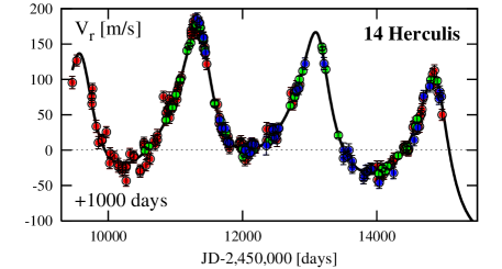
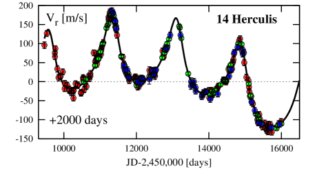
Figure 7: Synthetic RV data and the RV curve of the corresponding best fit to the two-planet model. The left panel is for the time series extended over 1000 days after the last real observation, the right panel is for the synthesized data over 2000 days after the last real data point. Sampling frequency and errors of the artificial observations are similar to those of the real data.

         

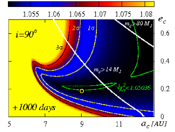
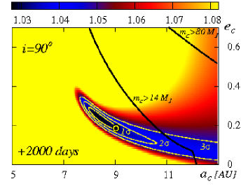
Figure 8: The topology of ${(\chi^{2}_{\nu})^{1/2}}$ in the $(a_{c},e_{c})$-plane of the best fits to the synthetic data sets shown in Fig. 7. The left panel is for artificial observations spanning additional 1000 days after the date of the last real data point, the right panel is for the additional 2000 days period. Contours mark $1\sigma,2\sigma$ and $3\sigma$-levels of ${(\chi^{2}_{\nu})^{1/2}}$. Thick lines (white in the left panel, black in the right panel) are for the mass limits of $14~{}\mbox{m}_{{\mbox{\scriptsize J}}}$ and $80~{}\mbox{m}_{{\mbox{\scriptsize J}}}$, respectively. Circle marks the position of the nominal best-fit in Table 1 (the “real” system).

5 Secular dynamics of the best-fit system

Although the RV data permit for different dynamical states of the system, we can analyse the secular evolution of the best fit coplanar and edge-on configuration (Table 1) and the solutions in its neighborhood. Due to the significant uncertainty of the orbital elements of outer planet, such analysis cannot provide exhaustive conclusions but we can obtain some qualitative view of the secular behaviour of the system. It can be easily extended when more RV data will be available.

As we have demonstrated, the parameters of the inner planet as well as the eccentricity and orbital phase of the putative outer companion can be relatively well constrained. The most unconstrained parameter in the edge-on, coplanar system is $a_{{\mbox{\scriptsize c}}}$. Yet we should remember that the observations constrain very roughly the inclinations; and we did not include the longitudes of nodes as free parameters in the model, keeping the planets in coplanar orbits. Still, we are in relatively a good situation because the careful analysis of the RV data makes it possible to reduce the dimension of the phase space. The dynamical map in Fig. 4 covering the shallow minimum of ${(\chi^{2}_{\nu})^{1/2}}$ and the neighborhood of the formal best fit reveals its proximity to the 11:2 MMR. Several authors argue that in similar cases, (Libert & Henrard, 2007, 2005; Rodríguez & Gallardo, 2005) in the first approximation the near-resonance effects have a small or negligible influence on the secular dynamics. Hence, neglecting the effects of the MMRs, we can recover its basic properties with the help of the recent quasi-analytical averaging method by Michtchenko & Malhotra (2004). It generalizes the classic Laplace-Lagrange (L-L) theory (Murray & Dermott, 2000) or a more recent work by Lee & Peale (2003). It relies on a semi-numerical averaging of the perturbing Hamiltonian and makes it possible to avoid any series expansions when recovering the secular variations of the orbital elements. Then one obtains a very accurate secular model which is valid up to large eccentricities by far beyond the limits of L-L classical theory. The details of this powerful approach can be found in (Michtchenko & Malhotra, 2004; Michtchenko et al., 2006).

To study the secular dynamics, we follow Michtchenko & Malhotra (2004) and describe the system in terms of the canonical Poincaré variables. First, we obtain the time-average of the canonical elements derived from the numerical integration of the full equations of motion with the initial condition in Table 1. The mean canonical semi-major axes of the system are then $\langle a_{{\mbox{\scriptsize b}}}\rangle\sim 2.868$ AU and $\langle a_{{\mbox{\scriptsize c}}}\rangle\sim 8.891$ AU. The eccentricities are $\langle e_{{\mbox{\scriptsize b}}}\rangle\sim 0.356$ and $\langle e_{{\mbox{\scriptsize c}}}\rangle\sim 0.191$. The initial state of the system is also characterized by the difference of arguments of periastron, $\Delta\varpi=\varpi_{{\mbox{\scriptsize b}}}-\varpi_{{\mbox{\scriptsize c}}}\sim 195^{\circ}$ with $1\sigma$ uncertainty $\sim 27^{\circ}$ that is estimated from the statistics of solutions derived for fixed masses and semi-major axes (parameters of the secular model), at their respective values in Table 1.

Next, we compute the energy levels of the averaged Hamiltonian of the system $\langle H_{{\mbox{\scriptsize sec}}}\rangle$ (Fig. 9, left panel) in the characteristic plane ($e_{{\mbox{\scriptsize b}}}\cos\Delta\varpi,e_{{\mbox{\scriptsize c}}}$) where $\Delta\varpi$ is set either to $0^{\circ}$ or $180^{\circ}$. Let us note that $\Delta\varpi$ always passes through these values during the orbital evolution related to two distinct libration modes of $\Delta\varpi$ in the coplanar system (Michtchenko & Malhotra, 2004). The energy level of the nominal system is marked with red line. The black thick lines mark the exact positions of libration centers (i.e., periodic solutions) of $\Delta\varpi$ around $0^{\circ}$ (mode I) and $180^{\circ}$ (mode II), respectively. A green part of the libration curve (on the right half-plane of the energy diagram) is for the nonlinear secular resonance of the system. The black dashed lines mark different levels of the total angular momentum (expressed by the Angular Momentum Deficit, $AMD$). The nominal system (marked with filled dots) is found in the region of the anti-aligned apsides (close to the thin curve representing mode II) with $e_{{\mbox{\scriptsize c}}}$ in the range $\sim(0.1,0.2)$.

To illustrate the secular dynamics in more detail, we computed the phase diagrams of the system in the characteristic plane of $(e_{{\mbox{\scriptsize b}}}\cos\Delta\varpi,e_{{\mbox{\scriptsize b}}}\sin\Delta\varpi)$ (the top-left panel in Fig 9) and in the $(e_{{\mbox{\scriptsize c}}}\cos\Delta\varpi,e_{{\mbox{\scriptsize c}}}\sin\Delta\varpi)$-plane (the bottom-left panel in Fig. 9). The red curves mark the oscillation around libration mode I, blue curves are for libration mode II and black curves mark the circulation of $\Delta\varpi$. The nominal system (marked with filled circles) lies close to the center of mode II with a relatively large amplitude of $e_{{\mbox{\scriptsize b}}}\sim 0.5$. The librations of $\Delta\varpi$ are confined to small semi-amplitudes $\sim 30^{\circ}$. The results of the secular theory are in an excellent accord with the behavior of the full unaveraged system. Its dynamical maps are shown in Fig. 4. The dynamical map of $\max\Delta\varpi$ (i.e., the maximal semi-amplitude of $\Delta\varpi$ attained during the integration time) reveals a similar semi-amplitude of librations $\sim 30^{\circ}$ around the center of $180^{\circ}$ (and of course, the presence of mode II). This zone persists over wide ranges of $(a_{{\mbox{\scriptsize c}}},e_{{\mbox{\scriptsize c}}})$. In fact, almost the entire stable region extending at least up to 11 AU is spanned by configurations involved in mode II librations. The error bars in plots of Fig. 9 are derived from formal estimates of $1\sigma$ errors of the parameters in Table 1 (we estimate the error of $\Delta\varpi\sim 27^{\circ}$; according with the analysis of stability, we adopted the uncertainty of $e_{c}$ as 0.15). The errors are significant but still, in the statistical sense, the libration modes would mostly not change within the error ranges. This behaviour is confirmed in Fig. 10 showing $\Delta\varpi$ for each individual best-fit found (see the top-left panel of Fig. 3). Simultaneously, physically stable systems are close to quasi-periodic configurations what follows from the comparison of the $\max e$ and $\max\Delta\varpi$ indicators. Both of them, as indicators of geometrical or physical behaviour of the system in short-time scale, appear tightly corelated to the $\log SN$ as the formal measure of the system stability.

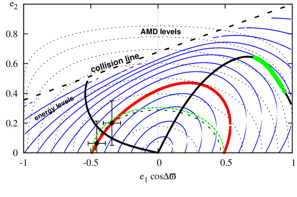
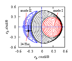
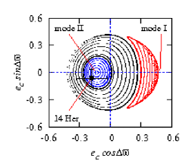
Figure 9: The secular evolution of the best-fit configuration (see Table 1). The left panel is for the energy levels of the averaged secular Hamiltonian $\langle H\rangle_{{\mbox{\scriptsize sec}}}$ (blue, continuous curves) and the $AMD$ levels (black, dashed lines) on the representative plane of initial conditions. The energy decreases and $AMD$ increases with increasing $e_{{\mbox{\scriptsize c}}}$. The sign of $e_{{\mbox{\scriptsize b}}}\cos\Delta\varpi$ is for initial conditions with $\Delta\varpi=0^{\circ}$ (+) or $\Delta\varpi=180^{\circ}$ (-), respectively. The level curves are computed for $m_{{\mbox{\scriptsize b}}}/m_{{\mbox{\scriptsize c}}}=0.648$ and $a_{{\mbox{\scriptsize b}}}/a_{{\mbox{\scriptsize c}}}=0.3226$. The red thick curve marks the energy level of the nominal system, and filled circles indicate actual variation of the eccentricities (through the angular momentum integral). The black thick lines mark the centers of librations of $\Delta\varpi$ around $0^{\circ}$ (mode I) or $180^{\circ}$ (mode II), respectively. A green region (on the right, for positive $e_{{\mbox{\scriptsize b}}}\cos\Delta\varpi$) is for the nonlinear secular resonance. Panels in the left column are for the secular phase space of the planets b and c at secular energy $\langle H\rangle_{{\mbox{\scriptsize sec}}}$ of the nominal system in the ($e_{{\mbox{\scriptsize b}}}\cos\Delta\varpi,e_{{\mbox{\scriptsize b}}}\sin\Delta\varpi)$-plane (the right-top panel) and ($e_{{\mbox{\scriptsize c}}}\cos\Delta\varpi,e_{{\mbox{\scriptsize c}}}\sin\Delta\varpi)$-plane (the right-bottom panel), respectively. Two libration modes of $\Delta\varpi$ about the centers $\Delta\varpi=0^{\circ}$ (mode I, red curves) and $\Delta\varpi=180^{\circ}$ (mode II, blue curves) are labeled. Thick black lines are for the transition between the libration and circulation of $\Delta\varpi$. Initial mean parameters of the nominal systems are marked with filled circles. For a reference, we plot formal error bars derived from $1\sigma$ errors of the best fit parameters in Table 1.

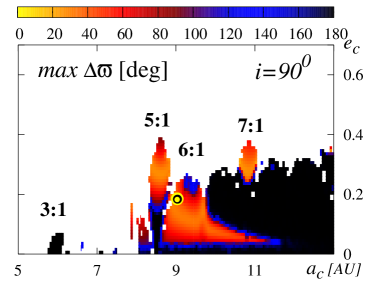
Figure 10: The dynamical map in the $(a_{{\mbox{\scriptsize c}}},e_{{\mbox{\scriptsize c}}})$-plane in terms of the $\max\Delta\varpi$ indicator for edge-on, coplanar system and assemble of fits shown in Fig. 3, the top-left panel. The large crossed circles mark the parameters of the best fit solution in Table 1. The low-order MMRs of the planets b and c are labeled. The integrations are conducted over $\sim 10^{4}P_{{\mbox{\scriptsize c}}}$.

6 Conclusions

According to the results from the adaptive-optics imaging (Luhman & Jayawardhana, 2002; Patience et al., 2002), there is no stellar-mass object in the 14 Her neighborhood beyond $\sim 12$ AU. This finding supports the hypothesis that the RV trend may be attributed to a massive planet c. The orbital period of the putative companion to the known Jovian planet b cannot yet be very well constrained. Nevertheless the available data already reveal a very shallow minimum od ${(\chi^{2}_{\nu})^{1/2}}$ in the ($a_{{\mbox{\scriptsize c}}},e_{{\mbox{\scriptsize c}}})$-plane of the initial osculating elements. The minimum persists for reasonable combinations of the parent star mass and the inclination of the system. Its dynamical character strongly depends on that parameter influencing the planetary masses. Quite surprisingly, for small inclinations the mass hierarchy is reversed and the inner planet becomes more massive than its distant companion. Also the positions of the nearby MMRs are significantly affected. Depending on the inclination, the system may be locked in the low-order 9:2, 5:1 or 6:1 MMR. We can also conclude that the kinematic model of the RV is already not adequate for the characterization of the system and further analysis of the RV would be done best within the self-consistent Newtonian model.

The dynamical analysis enables us to derive some limits on the orbits elements and the stability of the system. No stable configurations are found with a period ratio smaller than $\sim 3$. This limit is shifted towards larger values when the inclination grows. For the inclination of $30^{\circ}$, the best fit solutions are localized in a strongly chaotic and unstable zone. This constitutes a dynamically derived argument against a small inclination of the system. It is likely larger than $30^{\circ}$-$40^{\circ}$. Allowing for some speculation, the presence of the best-fits in a robustly stable zone supports the hypothesis of highly inclined two-planet configuration in the 14 Her system. Our attempts to fit one more planet to the RV data that could explain the scatter of the data points close to the minima of the RV curve (Fig. 5), did not lead to a meaningful improvement of the fit. The third planet would have a weak RV signal at the level of a few m/s and a short-period eccentric orbit. Finally, the analysis of all available RV data of 14 Her enables us to revise and extend some of the conclusions from Goździewski et al. (2006) — an isolated and very well defined best-fit solution cannot yet be found to properly describe the orbital configuration of 14 Her.

Acknowledgements. We thank Eric Ford for a critical review, suggestions and comments that greatly improved the manuscript. This work would not be possible without the access to the precision RV data which the discovery teams make available to the community. This work is supported by the Polish Ministry of Science and Education through grant 1P03D-021-29. M.K. is also supported by the Polish Ministry of Science and Education through grant N203 005 32/0449.

References

- Bevington & Robinson (2003) Bevington, P. R., Robinson, D. K, 2003 Data reduction and error analysis for the physical sciences, McGraw-Hill
- Butler et al. (2003) Butler R. P., Marcy G. W., Vogt S. S., Fischer D. A., Henry G. W., Laughlin G., Wright J. T., 2003, ApJ, 582, 455
- Butler et al. (2006) Butler R. P., Wright J. T., Marcy G. W., Fischer D. A., Vogt S. S., Tinney C. G., Jones H. R. A., Carter B. D., Johnson J. A., McCarthy C., Penny A. J., 2006, ApJ, 646, 505
- Charbonneau (1995) Charbonneau P., 1995, ApJs, 101, 309
- Cincotta & Simó (2000) Cincotta P. M., Simó C., 2000, Astron. Astroph. Suppl. Ser., 147, 205
- Ferraz-Mello et al. (2005) Ferraz-Mello S., Michtchenko T. A., Beaugé C., 2005, ApJ, 621, 473
- Goździewski & Konacki (2004) Goździewski K., Konacki M., 2004, ApJ, 610, 1093
- Goździewski et al. (2003) Goździewski K., Konacki M., Maciejewski A. J., 2003, ApJ, 594
- Goździewski et al. (2006) Goździewski K., Konacki M., Maciejewski A. J., 2006, ApJ, 645, 688
- Goździewski et al. (2005) Goździewski K., Konacki M., Wolszczan A., 2005, ApJ, 619, 1084
- Goździewski et al. (2007) Goździewski K., Maciejewski A. J., Migaszewski C., 2007, ApJ, 657, 546
- Goździewski & Migaszewski (2006) Goździewski K., Migaszewski C., 2006, A&A, 449, 1219
- Laughlin & Chambers (2001) Laughlin G., Chambers J. E., 2001, ApJ, 551, L109
- Lee et al. (2006) Lee M. H., Butler R. P., Fischer D. A., Marcy G. W., Vogt S. S., 2006, ApJ, 641, 1178
- Lee & Peale (2003) Lee M. H., Peale S. J., 2003, ApJ, 592, 1201
- Libert & Henrard (2005) Libert A.-S., Henrard J., 2005, Celestial Mechanics and Dynamical Astronomy, 93, 187
- Libert & Henrard (2007) Libert A.-S., Henrard J., 2007, A&A, 461, 759
- Luhman & Jayawardhana (2002) Luhman K. L., Jayawardhana R., 2002, ApJ, 566, 1132
- Michtchenko & Ferraz-Mello (2001) Michtchenko T., Ferraz-Mello S., 2001, ApJ, 122, 474
- Michtchenko et al. (2006) Michtchenko T. A., Ferraz-Mello S., Beaugé C., 2006, Icarus, 181, 555
- Michtchenko & Malhotra (2004) Michtchenko T. A., Malhotra R., 2004, Icarus, 168, 237
- Murray & Dermott (2000) Murray C. D., Dermott S. F., 2000, Solar System Dynamics. Cambridge Univ. Press
- Naef et al. (2004) Naef D., Mayor M., Beuzit J. L., Perrier C., Queloz D., Sivan J. P., Udry S., 2004, A&A, 414, 351
- Patience et al. (2002) Patience J., White R. J., Ghez A. M., McCabe C., McLean I. S., Larkin J. E., Prato L., Kim S. S., Lloyd J. P., Liu M. C., Graham J. R., Macintosh B. A., Gavel D. T., Max C. E., Bauman B. J., Olivier S. S., Wizinowich P., Acton D. S., 2002, ApJ, 581, 654
- Pepe et al. (2007) Pepe F., Correia A. C. M., Mayor M., Tamuz O., Couetdic J., Benz W., Bertaux J.-L., Bouchy F., Laskar J., Lovis C., Naef D., Queloz D., Santos N. C., Sivan J.-P., Sosnowska D., Udry S., 2007, A&A, 462, 769
- Press et al. (1992) Press W. H., Teukolsky S. A., Vetterling W. T., Flannery B. P., 1992, Numerical Recipes in C. The Art of Scientific Computing. Cambridge Univ. Press
- Rivera & Lissauer (2001) Rivera E. J., Lissauer J. J., 2001, ApJ, 402, 558
- Rodríguez & Gallardo (2005) Rodríguez A., Gallardo T., 2005, ApJ, 628, 1006
- Smart (1949) Smart W. M., 1949, Text-Book on Spherical Astronomy. Cambridge Univ. Press
- Vogt et al. (2005) Vogt S. S., Butler R. P., Marcy G. W., Fischer D. A., Henry G. W., Laughlin G., Wright J. T., Johnson J. A., 2005, ApJ, 632, 638
- Wittenmyer et al. (2007) Wittenmyer R. A., Endl M., Cochran W. D., 2007, ApJ, 654, 625