Recent progresses in the simulation of small-scale magnetic fields

Abstract

New high-resolution observations reveal that small-scale magnetic flux concentrations have a delicate substructure on a spatial scale of $0.1^{\prime\prime}$. Its basic structure can be interpreted in terms of a magnetic flux sheet or tube that vertically extends through the ambient weak-field or field-free atmosphere with which it is in mechanical equilibrium. A more refined interpretation comes from new three-dimensional magnetohydrodynamic simulations that are capable of reproducing the corrugated shape of magnetic flux concentrations and their signature in the visible continuum. Furthermore it is shown that the characteristic asymmetric shape of the contrast profile of facular granules is an effect of radiative transfer across the rarefied atmosphere of the magnetic flux concentration. I also discuss three-dimensional radiation magnetohydrodynamic simulations of the integral layers from the top of the convection zone to the mid-chromosphere. They show a highly dynamic chromospheric magnetic field, marked by rapidly moving filaments of stronger than average magnetic field that form in the compression zone downstream and along propagating shock fronts. The simulations confirm the picture of flux concentrations that strongly expand through the photosphere into a more homogeneous, space filling chromospheric field. Future directions in the simulation of small-scale magnetic fields are indicated by a few examples of very recent work.

1 Introduction

With “realistic simulations” computational physicists aim at imitating real physical processes that occur in nature. In the course of rebuilding nature in the computer, they aspire to a deeper understanding of the process under investigation. In some sense the opposite approach is taken by computational physicists that aim at separating the fundamental physical processes by abstraction from the particulars for obtaining “ideal simulations” or an analytical model of the essential physical process. Both strategies are needed and are complementary as can be seen for example in Section 4 on the physics of faculae. In this paper, however, we mainly focus on “realistic simulations” and comparison with observations.

The term small-scale flux concentration is used here to designate the magnetic field that appears in G-band filtergrams as bright tiny objects within and at vortices of intergranular lanes. They are also visible in the continuum, where they are called facular points (Mehltretter, 1974), while the structure made up of bright elements is known as the filigree (Dunn & Zirker, 1973). In more recent times, the small-scale magnetic field was mostly observed in the G band (a technique originally introduced by Muller, 1985) because the molecular band-head of CH that constitutes the G band acts as a leverage for the intensity contrast (Rutten, 1999; Rutten et al., 2001; Sánchez Almeida et al., 2001; Shelyag et al., 2004; Steiner et al., 2001). Being located in the blue part of the visible spectrum, this choice also helps improving the diffraction limited spatial resolution and the contrast in the continuum.

Small-scale magnetic flux concentrations are studied for several reasons:

• Since they make up the small end of a hierarchy of magnetic structures on the solar surface, the question arises whether they are “elemental” or whether yet smaller flux elements exist. How do they form? Are they a surface phenomenon? What is their origin?

• Near the solar limb they can be identified with faculae, known to critically contribute to the solar irradiance variation.

• They probably play a vital role in the transport of mechanical energy to the outer atmosphere, e.g., by guiding and converting magnetoacoustic waves generated by the convective motion and granular buffeting.

2 The basic structure of small-scale magnetic flux concentrations

Recent observations of unprecedented spatial resolution with the 1 m Swedish Solar Telescope by Berger et al. (2004) and Rouppe van der Voort et al. (2005) reveal G-band brightenings in an active region as delicate, corrugated ribbons that show structure down to the resolution capability of the instrument of $0.1^{\prime\prime}$, while isolated point-like brightenings exist as well. The structure made up of these objects evolves on a shorter than granular time-scale, giving the impression of a separate (magnetic) fluid that resists mixing with the granular material. Figure 1 shows an example G-band filtergram from the former paper taken in a remnant active region plage near disk center. In this region, intergranular lanes are often completely filled with magnetic field like in the case marked by the white lines in Fig. 1. There, and in other similar cases, the magnetic field concentration is framed by a striation of bright material, while the central part is dark. Figure 1 shows examples of ribbon bands and also an isolated bright point in the lower right corner.

The graphic to the right hand side of Fig. 1 displays the emergent G-band intensity (solid curve) from the cross section marked by the white horizontal lines in the image to the left. Also shown are the corresponding magnetographic signal (dashed curve), the blue continuum intensity (dotted), and the Ca H-line intensity (dash-dotted). Note that the magnetic signal is confined to the gap between the two horizontal white lines. The intensities show a two-humped profile.

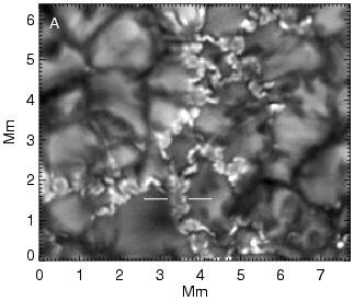
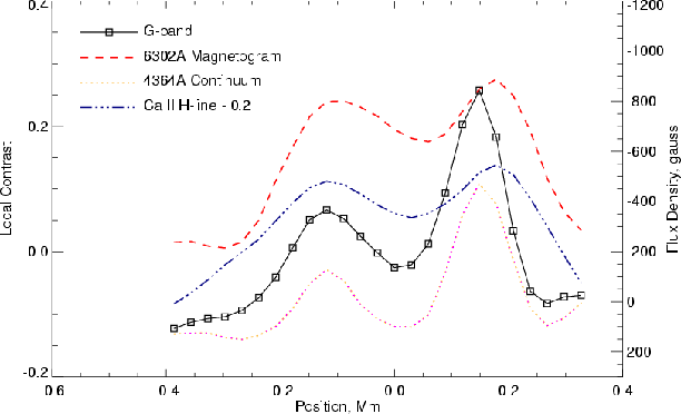
Figure 1: Left: G-band filtergram showing the ribbon-like shape of magnetic flux concentrations. Right: G-band intensity (solid curve) along the section indicated by the horizontal white lines in the image to the left. Also shown are the magnetogram signal, the continuum intensity at 436.4 nm, and the Ca II H-line intensity down-shifted by 0.2. From Berger et al. (2004).

This situation reminds of the flux-sheet model and the “bright wall effect”. A first quasi-stationary, self-consistent simulation of a small-scale flux sheet was carried out by Deinzer et al. (1984a, b), popularly known as the “KGB-models”. The basic properties of this model are sketched in Fig. 2. Accordingly, a small-scale flux concentration, either of tube or sheet-like shape, is in mechanical equilibrium with the ambient atmosphere, viz., the gas plus magnetic pressure of the atmosphere within the tube/sheet balances the gas pressure in the ambient (field-free) medium at equal geometrical height. This situation calls for a reduced density in the flux concentration with respect to the environment, at least in the photospheric part, where the radiative heat exchange quickly drives the configuration towards radiative equilibrium, hence to a similar temperature at constant geometrical height. This density reduction renders the flux tube/sheet atmosphere more transparent, which causes a depression of the surface of constant optical depth, as indicated by the surface of $\tau_{c}=1$ in Fig. 2. In a plage or network region, this effect increases the “roughness” of the solar surface, hence the effective surface from which radiation can escape, which increases the net radiative loss from these areas.

The graphics to the right hand side of Fig. 2 shows a sketch of the relative intensity emerging from this model, viz., the intensity of light propagating in the vertical direction as a function of distance from the flux sheet’s plane of symmetry. It corresponds to the plot on the right hand side of Fig. 1. The similarity between this model and the observation is striking. Turning to a narrower flux sheet/tube would result in the merging of the two contrast peaks to a single central peak in both, model and observation, i.e., to a ribbon band or bright point, respectively. Yet, the striation of the depression wall that can be seen in the observation is of course not reproduced by the model, which is strictly two-dimensional with translational invariance in lane direction. We will see in Sect. 4 that three-dimensional magnetoconvection simulations show rudimentary striation. The physical origin of the striation is still unknown.

Accordingly, the basic properties of ribbon-like magnetic flux concentrations can be understood in terms of a magnetic flux sheet embedded in and in force balance with a more or less field-free ambient medium. This can also be said (replacing the word sheet by tube) of the rosette structure visible in other still images of Berger et al. (2004) who call it “flower-like”. Flowers can transmute to pores and vice versa. The striation of their bright collar is similar to that seen in ribbon structures. Discarding the striation, the basic properties of flowers can well be interpreted in terms of a tube shaped flux concentration like the one sketched in Fig. 2.

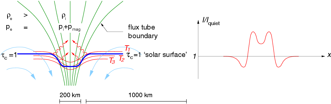
Figure 2: Sketch of a magnetic flux sheet (left) with corresponding intensity contrast (right), distilled from self-consistent numerical MHD simulations. Note that the isothermal surfaces are not exactly parallel to the surface of optical depth unity, which gives rise to the particular M-shape of the contrast profile.

A 2 h sequence of images with a quality comparable to Figs. 1 (Rouppe van der Voort et al., 2005) reveals that the shape of the ribbon-like flux concentrations and the striation of ribbons and flowers change on a very short time-scale, of the order of the Alfvén crossing travel time. This suggests that these morphological changes and the striation itself are related to the flute instability, which small-scale flux concentrations are liable to. For an untwisted axisymmetric flux tube, the radial component of the magnetic field at the flux-tube surface must decrease with height, $\left.{\rm d}B_{r}/{\rm d}z\right|_{S}<0$, in order that the flux tube is stable against the flute (interchange) instability (Meyer et al., 1977). While sunspots and pores with a magnetic flux in excess of $\Phi\approx 10^{19}$ Mx do meet this condition, small-scale flux concentrations do not fulfill it (Schüssler, 1984; Steiner, 1990; Bünte et al., 1993). Bünte (1993) shows that small-scale flux sheets too are flute unstable, and he concludes that filament formation due to the flute instability close to the surface of optical depth unity would ensue. As the flux sheet is bound to fall apart because of the flute instability, its debris are again reassembled by the continuous advection back to the intergranular lane so that a competition between the two effects is expected to take place, which might be at the origin of the corrugation of the field concentrations and of the striation of the tube/sheet interface with the ambient medium.

Although the fine structure of small-scale magnetic flux concentrations changes on a very short time scale, single flux elements seem to persist over the full duration of the time sequence of 2 h. They may dissolve or disappear for a short period of time, but it seems that the same magnetic flux continually reassembles to make them reappear nearby. Latest G-band time sequences obtained with the Solar Optical Telescope (SOT) on board of the Japanese space satellite HINODE (http://solarb.msfc.nasa.gov/movies.html) seem to confirm these findings even for G-band bright points of low intensity. This suggest a deep anchoring of at least some of the flux elements although numerical simulation seem not to confirm this conjecture.

As indicated in the sketch of Fig. 2, the magnetic flux concentration is framed by a downflow of material, fed by a horizontal flow that impinges on the flux concentration. Already the flux-sheet model of Deinzer et al. (1984b) showed a persistent flow of this kind. According to these authors it is due to radiative cooling from the depression walls of the magnetic flux concentrations (the “hot wall effect”) that causes a horizontal pressure gradient, which drives the flow. The non-stationary flux-sheet simulations of Steiner et al. (1998) and Leka & Steiner (2001) showed a similar persistent downflow, which, with increasing depth, becomes faster and narrower, turning into veritable downflow jets beneath the visible surface. While downflows in the periphery of pores have been observed earlier (Leka & Steiner, 2001; Sankarasubramanian & Rimmele, 2003; Tritschler et al., 2003) and also horizontal motions towards a pore by Dorotovič et al. (2002), only very recently such an accelerating downflow has been observationally detected in the immediate vicinity of ribbon bands by Langangen et al. (2007).

3 3-D simulations of small-scale magnetic flux concentrations

New results from realistic simulations on the formation, dynamics and structure of small-scale magnetic flux concentrations have recently been published in a series of papers by Schüssler and collaborators. Vögler et al. (2005) simulate magnetoconvection in a box encompassing an area on the solar surface of $6\times 6$ Mm² with a height extension of 1400 km, reaching from the temperature minimum to 800 km below the surface of optical depth unity. Although this is only 0.4% of the convection zone depth, the box still includes the entire transition from almost completely convective to mainly radiative energy transfer and the transition from the regime where the flux concentration is dominated by the convective plasma flow to layers where the magnetic energy density of the flux concentrations by far surpasses the thermal energy density. The bottom boundary in this and similar simulations is open in the sense that plasma can freely flow in and out of the computational domain, subject to the condition of mass conservation. Inflowing material has a given specific entropy that determines the effective temperature of the radiation leaving the domain at the top, while the outflowing material carries the entropy it instantly has.

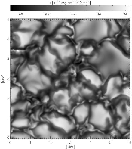
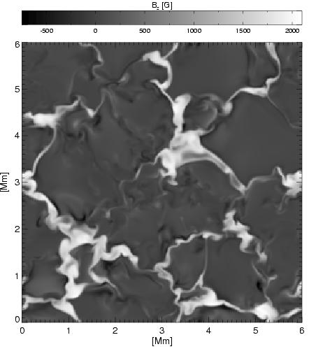
Figure 3: Simulation snapshot. Left: Frequency integrated intensity. Right: Vertical magnetic flux density at constant average geometrical height of optical depth unity. The mean flux density is 200 G. From Vögler et al. (2005).

Figure 3 shows a snapshot from this simulation: To the left the emergent mean intensity, to the right the vertical magnetic field strength at a constant height, viz., at the horizontally averaged geometrical height of optical depth unity. (I would like to caution that this magnetic map is not what would be seen with a magnetograph, irrespective of its spatial resolution.) The strong magnetic field in intergranular lanes is manifest in a corresponding signal in the emergent intensity very much like the snapshot discussed in Sect. 2. Also the intensity signal shows the same corrugated and knotted ribbon structure that is observed, and sometimes there appear also broader ribbon structures with a dark central core, like the one marked in Fig. 1. In the latter case however, the characteristic striation is absent, possibly because the flute instability is suppressed on very small spatial scales due to lack of sufficient resolution of the simulation. In the central part of the snapshot, a micro pore or magnetic knot has formed.

A comparison of the average gas plus magnetic pressure as a function of height at locations of magnetic flux concentrations with the run of the average gas pressure in weak-field regions reveals that the two are almost identical, proving that even in this dynamic regime, the thin flux tube approximation is very well satisfied (Vögler et al., 2005). This result confirms that the model discussed in Sect. 2 and sketched in Fig. 2 is indeed an acceptable first approximation to the real situation.

Simulations are not just carried out for the sake of reproducing observed quantities. Once good agreement with all kind of observations exists, simulations allow with some confidence to inform about regions not directly accessible to observations, for example about the magnetic structure in subsurface layers. In this respect the simulations of Vögler et al. (2005) show that often flux concentrations that have formed at the surface disperse again in shallow depths. This behaviour was also found by Schaffenberger et al. (2005) in their simulation with an entirely different code and further by Stein & Nordlund (2006a). A vertical section through a three-dimensional simulation domain of Schaffenberger et al. (2005), where two such shallow flux concentrations have formed, is shown in Fig. 8. The superficial nature of magnetic flux concentrations in the simulations, however, is difficult to reconcile with the observation that many flux elements seem to persist over a long time period.

4 The physics of faculae

With growing distance from disk center, small-scale magnetic flux concentrations grow in contrast against the quiet Sun background and become apparent as solar faculae close to the limb. Ensembles of faculae form plage and network faculae that are as conspicuous features of the white light solar disk, as are sunspots. It is therefore not surprising that they play a key role in the solar irradiance variation over a solar cycle and on shorter time scales (Fligge et al., 2000; Wenzler et al., 2005; Foukal et al., 2006). Measurements of the center to limb variation of the continuum contrast of faculae are diverse, however, as the contrast is not only a function of the heliocentric angle, $\mu=\cos\theta$, but also of facular size, magnetic field strength, spatial resolution, etc., and as measurements are prone to selection effects. While many earlier measurements report a contrast maximum around $\mu\approx 0.2\ldots 0.4$ with a decline towards the limb, latest measurements (Sütterlin et al., 1999; Ahern & Chapman, 2000; Adjabshirizadeh & Koutchmy, 2002; Ortiz et al., 2002; Centrone & Ermolli, 2003; Vogler et al., 2005) point rather to a monotonically increasing or at most mildly decreasing contrast out to the limb.

The standard facula model (Spruit, 1976), again consists of a magnetic flux concentration embedded in and in mechanical equilibrium with a weak-field or field-free environment as is sketched in Fig, 2. When approaching the limb, the limb side of the bright depression wall becomes ever more visible and ever more perpendicular to the line of sight, which increases its brightness compared to the limb darkened environment. At the extreme limb, obscuration by the centerward rim of the depression starts to take place, which decreases the size and possibly the contrast of the visible limb-side wall.

Recently, Lites et al. (2004) and Hirzberger & Wiehr (2005) have obtained excellent images of faculae with the 1 m Swedish Solar Telescope. Figure 4 (from Hirzberger & Wiehr 2005) shows on the left hand side network faculae at a heliocentric angle of $\mu=0.48$ in the continuum at 587.5 nm. The solar limb is located towards the right hand side. It is clearly visible from this image that faculae are in reality partially brightened granules with an exceptionally dark and wide intergranular lane (“dark facular lane”) on the disk-center side of the contrast enhancement, which is also the location of the magnetic flux concentration. The right half of Fig. 4 shows the string of faculae within the white box of the image to the left, aligned according to the position of the dark lane. Also shown is the mean contrast profile, averaged over the alignment. Similar contrast profiles of single faculae are shown by Lites et al. (2004). Such contrast profiles pose now a new constraint that any model of faculae must satisfy.

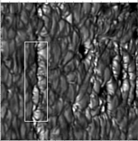
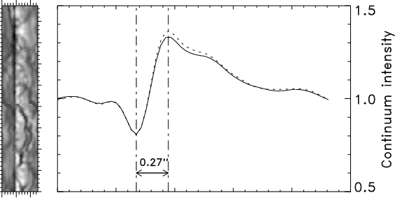
Figure 4: Left: Network faculae at a heliocentric angle of $\mu=0.48$ in the continuum at 587.5 nm. The solar limb is to the right. Right: Faculae within the white box of the image to the left aligned according to the position of the dark lane, together with the mean spatial scan through the aligned faculae. From Hirzberger & Wiehr (2005).

Magnetoconvective simulations as the one discussed in Sect. 3 indeed show facular-like contrast enhancements when computing the emergent intensity along lines of sight that are inclined to the vertical direction for mimicking limb observation. Such tilted three-dimensional simulation boxes are shown in the papers by Keller et al. (2004), Carlsson et al. (2004), and De Pontieu et al. (2006). Keller et al. (2004) also show the contrast profile of two isolated “faculae”, which however have a more symmetric shape, rather than the observed characteristic steep increase on the disk-center side with the gentle decrease towards the limb. Also they obtain a maximum contrast of 2, far exceeding the observed value of about 1.3. It is not clear what the reason for this discrepancy might be. Interestingly, the old “KGB-model” (Deinzer et al., 1984b; Knölker & Schüssler, 1988) as well as the two-dimensional, non-stationary simulation of Steiner (2005) do nicely reproduce the asymmetric shape and the dark lane.

Another conspicuous property of faculae that high-resolution images reveal is that they are not uniformly bright but show a striation not unlike to and possibly in connection with the one seen in G-band ribbons at disk center. While this feature cannot be reproduced in a two-dimensional model, it must be part of a satisfactory three-dimensional model. But so far 3-D simulations show only a rudimentary striation. This finding, rather surprisingly, indicates that the effective spatial resolution of present-day three-dimensional simulations is inferior to the spatial resolution of best current observations.

In an attempt to better understand the basic properties of faculae, Steiner (2005) considers the ideal model of a magnetohydrostatic flux sheet embedded in a plane parallel standard solar atmosphere. For the construction of this model the flux-sheet atmosphere is first taken to be identical to the atmosphere of the ambient medium but shifted in the downward direction by the amount of the “Wilson depression” (the depression of the surface of continuum optical depth unity at the location of the flux concentration). The shifting results in a flux-tube atmosphere that is less dense and cooler than the ambient medium at a fixed geometrical height. In the photospheric part of the flux concentration, thermal equilibrium with the ambient medium is then enforced. Denoting with index $i$ the flux-sheet atmosphere and with $e$ the ambient atmosphere and with $W$ the depth of the “Wilson depression”, we therefore have

$$T_{i}(z)=\!\!\left\{\!\!\!\begin{array}[]{l}T_{e}(z+W)\quad\mbox{for}\quad\tau_{c}\gg 1\\ T_{e}(z)\quad\mbox{for}\quad\tau_{c}\ll 1\;,\end{array}\right.$$ (1)

where $\tau_{c}$ is the optical depth in the visible continuum and $\rho_{i}(z)<\rho_{e}(z)\;\forall z$. The lower left panel of Fig. 5 shows this configuration together with two surfaces of optical depth unity, one for vertical lines of sight (disk center), the other for lines of sight running from the top right to the bottom left under an angle of $\theta=60^{\circ}$ to the vertical, like the one indicated in the figure. The upper left panel shows the corresponding continuum enhancement for disk center (double humped profile) and $\theta=60^{\circ}$. Of the curve belonging to $\theta=60^{\circ}$, all values left of the black dot belong to lines of sight left of the one indicated in the lower panel. This means that the contrast enhancement extends far beyond the depression proper in the limbward direction, exactly as is observed. The reason for this behaviour is explained with the help of Fig. 6 as follows.

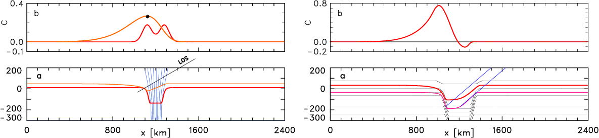
Figure 5: Left: a) Magnetic flux concentration (blue, vertically oriented lines of force, see internet version for colours) with surfaces of optical depth $\tau=1$ for vertical lines of sight (thick/red curve) and lines of sight inclined by $\theta=60^{\circ}$ to the vertical direction (thin/red curve). b) Corresponding contrast curves. All values of the light red curve left of the black dot originate from lines of sight left of the one indicated in panel a). Right: a) Surfaces of optical depth $\tau=1$ and $5$ (thick/red) for lines of sight inclined by $50^{\circ}$ to the vertical, together with isotherms. b) Contrast profile. The region of negative contrast is bounded by the two oblique lines of sight indicated in panel a).

A material parcel located in the solar atmosphere and lateral to the flux sheet “sees” a more transparent atmosphere in the direction toward the flux sheet compared to a direction under equal zenith angle but pointing away from it because of the rarefied flux-sheet atmosphere. Correspondingly, from a wide area surrounding the magnetic flux sheet or flux tube, radiation escapes more easily in the direction towards the flux sheet so that a single flux sheet/tube impacts the radiative escape in a cross-sectional area that is much wider than the magnetic field concentration proper.

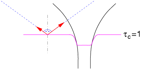
Figure 6: Photons preferentially escape along the line of sight to the right that traverses the magnetic flux sheet/tube in comparison to the line of sight to the left under equal zenith angle, because of the rarified (less opaque) atmosphere in the flux sheet/tube.

The right hand side of Fig. 5 shows a similar situation as to the left but for a flux sheet that is twice as wide. The continuum contrast for lines of sight inclined by $\theta=50^{\circ}$ to the vertical is shown in the top panel. It can be seen that a dark lane of negative contrast occurs on the disk-center side of the facula. It arises from the low temperature gradient of the flux-sheet atmosphere in the height range of $\tau_{c}=1$ and its downshift relative to the external atmosphere in combination with the inclined lines of sight. One could say that the dark lane in this case is an expression of the cool “bottom” of the magnetic flux sheet.

It is remarkable that this basic, energetically not self-consistent model is capable of producing both, the facular dark lane and the asymmetrically shaped contrast curve of the facula, with realistic contrast values. The results of this basic hydrostatic model carry over to a fully self-consistent model of a magnetic flux sheet in dynamic interaction with non-stationary convective motion (Steiner, 2005). In this case the facular lane becomes broader and darker.

It follows from these insights that a facula is not to be identified with bright plasma that sticks, as the name may insinuate, like a torch out of the solar surface and as the “hillock model” of Schatten et al. (1986) suggests. Rather is it the manifestation of photospheric granulation, seen across a magnetic flux concentration — granulation that appears brighter than normal in the form of so called “facular granules”. Interestingly, already Chevalier (1912) wondered: “La granulation que l’on voit autour des taches plus éclatante que sur les autres parties est-elle la granulation des facules ou celle de la photosphère vue à travers les facules ?” and Ten Bruggencate (1940) noted that “Sie [Photosphärengranulen und Fackelgranulen] unterscheiden sich nicht durch ihre mittlere Grösse, wohl aber durch den Kontrast gegenüber der Umgebung.”

If this is true, one expects facular granules to show the same dynamic phenomena like regular granulation. Indeed, this is confirmed in a comparison of observations with three-dimensional simulations by De Pontieu et al. (2006). They observe that often a dark band gradually moves from the limb side of a facula toward the disk center and seemingly sweeps over and ”erases” the facula temporarily. The same phenomenon they also observed in a time sequence of a three-dimensional simulation, which enabled them to identify the physics behind this phenomenon.

Examination of the simulation sequence reveals that dark bands are a consequence of the evolution of granules. Often granules show a dark lane that usually introduces fragmentation of the granule. The smaller fragment often dissolves (collapses) in which case the dark lane disappears with the collapsing small fragment in the intergranular space. Exactly this process can lead to the dark band phenomenon, when a granular dark lane is swept towards the facular magnetic flux concentration. Since the facular brightening is seen in the disk-center facing side of granules, only granular lanes that are advected in the direction of disk center lead to facular dimming. This example nicely demonstrates how regular granular dynamics when seen across the facular magnetic field can lead to genuine facular phenomena.

Despite the major progress that we have achieved in understanding the physics of faculae over the past few years, open questions remain. These concern

• a comprehensive model of the center to limb variation of the brightness of faculae including dependence on size, magnetic flux, flux density, color, etc.,

• a quantitative agreement between simulation and observation with respect to measurements in the infrared and with respect to the observed geometrical displacement between line core and continuum filtergrams of faculae,

• the physical origin of the striation,

• a quantitative evaluation of the heat leakage caused by faculae, or

• the role of faculae in guiding magnetoacoustic waves into the chromosphere.

5 3-D MHD simulation from the convection zone to the chromosphere

For investigating the connection between photospheric small scale magnetic fields and the chromosphere, Schaffenberger et al. (2005) have extended the three-dimensional radiation hydrodynamics code CO⁵BOLD  to magnetohydrodynamics for studying magnetoconvective processes in a three-dimensional environment that encompasses the integral layers from the top of the convection zone to the mid chromosphere. The code is based on a finite volume scheme, where fluxes are computed with an approximate Riemann-solver (LeVeque et al., 1998; Toro, 1999) for automatic shock capturing. For the advection of the magnetic field components, a constrained transport scheme is used.

The three-dimensional computational domain extends from 1400 km below the surface of optical depth unity to 1400 km above it and it has a horizontal dimension of $4800\times 4800$ km. The simulation starts with a homogeneous, vertical, unipolar magnetic field of a flux density of 10 G superposed on a previously computed, relaxed model of thermal convection. This low flux density is representative for magnetoconvection in a very quiet network-cell interior. The magnetic field is constrained to have vanishing horizontal components at the top and bottom boundary, but lines of force can freely move in the horizontal direction, allowing for flux concentrations to extend right to the boundaries. Because of the top boundary being located at mid-chromospheric heights, the magnetic field is allowed to freely expand with height through the photospheric layers into the more or less homogeneous chromospheric field.

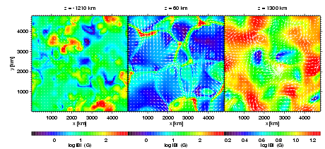
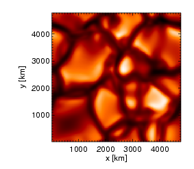
Figure 7: Horizontal sections through the three-dimensional computational domain. Color coding displays $\log|B|$ with individual scaling for each panel (see internet version for colours). Left: Bottom layer at a depth of 1210 km. Middle: Layer 60 km above optical depth $\tau_{c}=1$. Right: Top, chromospheric layer in a height of 1300 km. White arrows indicate the horizontal velocity on a common scaling. Longest arrows in the panels from left to right correspond to 4.5, 8.8, and 25.2 km/s, respectively. Rightmost: Emergent visible continuum intensity. From Schaffenberger et al. (2005).

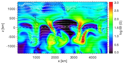
Figure 8: Snapshot of a vertical section through the three-dimensional computational domain, showing $\log|B|$ (color coded) and velocity vectors projected on the vertical plane (white arrows). The b/w dashed curve shows optical depth unity and the dot-dashed and solid black contours $\beta=1$ and 100, respectively. See internet version for colours. From Schaffenberger et al. (2005).

Figure 7 shows the logarithmic absolute magnetic flux density in three horizontal sections through the computational domain at a given time instant, together with the emergent Rosseland mean intensity. The magnetic field in the chromospheric part is marked by strong dynamics with a continuous rearrangement of magnetic flux on a time scale of less than 1 min, much shorter than in the photosphere or in the convection-zone layers. There, the field has a strength between 2 and 40 G in the snapshot of Fig. 7, which is typical for the whole time series. Different from the surface magnetic field, it is more homogeneous and practically fills the entire space so that the magnetic filling factor in the top layer is close to unity. There seems to be no spatial correlation between chromospheric flux concentrations and the small-scale field concentrations in the photosphere.

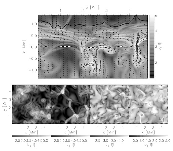
Figure 9: Logarithmic current density, $\log|j|$, in a vertical cross section (top panel) and in four horizontal cross sections in a depth of 1180 km below, and at heights of 90 km, 610 km, and 1310 km above the mean surface of optical depth unity from left to right, respectively. The arrows in the top panel indicate the magnetic field strength and direction. The dashed line indicates the position of the vertical section. [$j$] = $3\,\times\,10^{5}$ A/m². From Wedemeyer-Böhm et al. (2007).

Comparing the flux density of the panel corresponding to $z=60$ km with the emergent intensity, one readily sees that the magnetic field is concentrated in intergranular lanes and at lane vertices. However, the field concentrations do not manifest a corresponding intensity signal like in Fig. 3. This is because the magnetic flux is too weak to form a significant “Wilson depression” (as can be seen from Fig. 8) so that no radiative channeling effect takes place.

Figure 8 shows the logarithm of the absolute field strength through a vertical section of the computational domain. Overplotted are white arrows indicating the velocity field. The b/w dashed curve corresponds to the optical depth unity for vertical lines of sight. Contours of the ratio of thermal to magnetic pressure, $\beta$, for $\beta=1$ (dot-dashed) and $\beta=100$ (solid) are also shown. Magnetoacoustic waves that form transient filaments of stronger than average magnetic field are a ubiquitous phenomenon in the chromosphere and are also present in the snapshot of Fig. 8, e.g., along the contour of $\beta=1$ near $x=1200$ km and $x=2500$ km. They form in the compression zone downstream and along propagating shock fronts. These magnetic filaments that have a field strength rarely exceeding 40 G, rapidly move with the shock fronts and quickly form and dissolve with them.

The surface of $\beta=1$ separates the region of highly dynamic magnetic fields around and above it from the more slowly evolving field of high beta plasma below it. This surface is located at approximately 1000 km but it is corrugated and its local height strongly varies in time.

A very common phenomenon in this simulation is the formation of a ‘magnetic canopy field’ that extends in a more or less horizontal direction over expanding granules and between photospheric flux concentrations. The formation of such canopy fields proceeds by the action of the expanding flow above granule centres. This flow transports ‘shells’ of horizontal magnetic field to the upper photosphere and lower chromosphere, where shells of different field directions may be pushed close together, leading to a complicated network of current sheets in a height range from approximately 400 to 900 km.

This network can be seen in Fig. 9 (top), which shows, for a typical snapshot of the simulation, the logarithmic current density, $\log|j|$, together with arrows indicating the magnetic field strength and direction. Figure 9 (bottom) shows from left to right $\log|j|$ in four horizontal cross sections in a depth of 1180 km below, and at heights of 90 km, 610 km, and 1310 km above the mean surface of optical depth unity. Higher up in the chromosphere (rightmost panel), thin current sheets form along shock fronts, e.g., in the lower left corner near $x=1.4$ Mm.

Using molecular values for the electrical conductivity, Wedemeyer-Böhm et al. (2007) derive an energy flux of 5 to 50 W m^-2 into the chromosphere caused by ohmic dissipation of these current sheets. This value is about two orders of magnitude short of being relevant for chromospheric heating. On the other hand, the employed molecular values for the conductivity might be orders of magnitude too high for to be compatible with the effective electrical conductivity of the numerical scheme determined by the inherent artificial diffusion. Therefore, the ohmic heat flux might be conceivably two orders of magnitude larger than suggested by this rough estimate, so that magnetic heating by ohmic dissipation must be seriously taken into account. More advanced simulations, taking explicit ohmic diffusion into account will clarify this issue.

6 Future directions

Continuously increasing power of computational facilities together with steadily improving computational methods, expand the opportunity for numerical simulations. On the one hand, more detailed physics can be included in the simulation, on the other hand either the computational domain or the spatial and temporal resolution can be increased. In most simulations, especially when the computational domain encompasses only a small piece of a star, boundary conditions play an important role. They convey information on the outside world to the physical domain of the simulation. But this outside world is often poorly known. In order to acquire experience and intuition with respect to the influence of different types of boundary condition on the solution, one can implement and run various realizations of boundary conditions, which however also requires additional resources in computer power and time. Also the initial condition may critically determine the solution, for example the net flux and flux density of an initial, homogeneous vertical magnetic field. Boundary conditions, therefore, remain a hot topic also in future.

Most excitement in carrying out numerical simulations comes from the prospect of performing experiments with the object under investigation: experiments in the numerical laboratory. Not only that an astrophysical object can be reconstructed and simulated in the virtual world of the numerical laboratory. Once in the computer, the computational astrophysicist has the prospect of carrying out experiments with it as if the celestial body was taken to the laboratory.

The following few examples shall illustrate some aspects of this.

6.1 More detailed physics

In the solar chromosphere the assumption of LTE (local thermodynamic equilibrium) is not valid. Even the assumption of statistical equilibrium in the rate equations is not valid because the relaxation time-scale for the ionization of hydrogen approaches and surpasses the hydrodynamical time scale in the chromosphere (Kneer, 1980). Yet, in order to take time dependent hydrogen ionization in a three-dimensional simulation into account, simplifications are needed. Leenaarts & Wedemeyer-Böhm (2006) employ the method of fixed radiative rates for a hydrogen model atom with six energy levels in the three-dimensional radiation (magneto-)hydrodynamics code CO⁵BOLD. Thus, additional to the hydrodynamic equations, they solve the time-dependent rate equations

$$\frac{\partial n_{i}}{\partial t}+\nabla\cdot(n_{i}\mbox{\boldmath v})=\sum_{j\neq i}^{n_{l}}n_{j}P_{ji}-n_{i}\sum_{j\neq i}^{n_{l}}P_{ij}\,,$$ (2)

with $P_{ij}$ being the sum of collisional and radiative rate coefficients, $P_{ij}=C_{ij}+R_{ij}$. The rate coefficients are now local quantities given a fixed radiation field for each transition, which is obtained from one-dimensional test calculations.

Simulations with this approach show that above the height of the classical temperature minimum, the non-equilibrium ionization degree is fairly constant over time and space at a value set by hot propagating shock waves. This is in sharp contrast to results with LTE, where the ionization degree varies by more than 20 orders of magnitude between hot gas immediately behind the shock front and cool regions further away. The addition of a hydrogen model atom provides realistic values for hydrogen ionization degree and electron density, needed for detailed radiative transfer diagnostics.

6.2 Large box simulations

Benson et al. (2007) have carried out first simulations with a large simulation box so as to accommodate a supergranulation cell. They started a simulation that encompasses a volume of $48\times 48\times 20$ Mm³ using $500^{3}$ grid cells. With this simulation they hope to find out more about the origin of supergranulation and to carry out helioseismic experiments (Zhao et al., 2007).

Hansteen (2004) has carried out MHD simulations comprising a vast height range from the top layers of the convection zone into the transition region and the corona. With these simulations they seek to investigate various chromospheric features such as dynamic fibrils (Hansteen et al., 2006), mottles, and spicules, which are some of the most important, but also most poorly understood, phenomena of the Sun’s magnetized outer atmosphere. But also the transition zone and coronal heating mechanisms are in the focus of these kinds of “holistic” simulations.

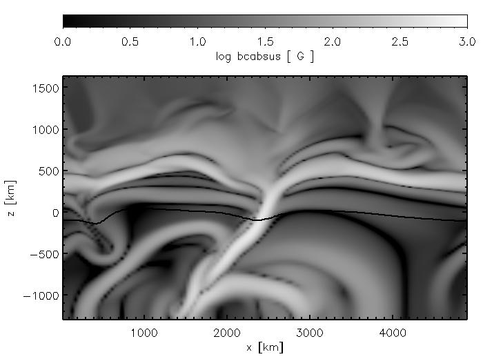
Figure 10: Left: Still image of the logarithmic magnetic flux density from a time series for the instant $t=1368$ s after starting with an initial homogeneous vertical field of 10 G flux density. A strong magnetic flux sheet has formed extending from $(x,z)\approx(2000,-500)$ to $(x,z)\approx(2500,0)$. Right: A plane parallel wave with frequency 100 mHz travels through convecting plasma into the magnetically structured photosphere and further into the low $\beta$ (magnetically dominated) chromosphere. The panel shows the difference in absolute velocity between the perturbed and the unperturbed solution 212 s after the start of the perturbation. The wave becomes strongly refracted in the low $\beta$ region and at the location of the flux sheet.

6.3 Improvements in boundary conditions

Many conventional magnetohydrodynamic simulations of the small-scale solar magnetic field assume that the horizontal component of the magnetic field vanishes at the top and bottom of the computational domain (e.g. Weiss et al., 1996; Cattaneo et al., 2003; Vögler et al., 2005; Schaffenberger et al., 2005), which is a rather stark constraint, especially with respect to magnetoacoustic wave propagation and Poynting flux. Recently, Stein & Nordlund (2006b) have introduced an alternative condition with the possibility of advecting magnetic field across the bottom boundary. Thus, upflows into the computational domain carry horizontal magnetic field of a prescribed flux density with them, while outflowing plasma carries whatever magnetic field it instantly has. With this condition an equilibrium in which equal amounts of magnetic flux are transported in and out of the computational domain is approached after some time. It should more faithfully model the plasma flow across the lower boundary and it allows for the effect of magnetic pumping (Tobias et al., 1998).

6.4 Helioseismic experiment with a magnetically structured atmosphere

With numerical experiments Steiner et al. (2007) have explored the feasibility of using high frequency waves for probing the magnetic fields in the photosphere and the chromosphere of the Sun. They track an artificially excited, plane-parallel, monochromatic wave that propagates through a non-stationary, realistic atmosphere, from the convection-zone through the photosphere into the magnetically dominated chromosphere, where it gets refracted and reflected.

When comparing the wave travel time between two fixed geometrical height levels in the atmosphere (representing the formation height of two spectral lines) with the topography of the surface of equal magnetic and thermal energy density (the magnetic canopy or $\beta=1$ surface) we find good correspondence between the two. These numerical experiments support expectations by Finsterle et al. (2004) that high frequency waves bear information on the topography of the ‘magnetic canopy’. This simulation exemplifies how a piece of Sun can be made accessible to virtual experimenting by means of realistic numerical simulation.

References

- Adjabshirizadeh & Koutchmy (2002) Adjabshirizadeh, A. & Koutchmy, S. 2002, in ESA SP-506: Solar Variability: From Core to Outer Frontiers, 415–418
- Ahern & Chapman (2000) Ahern, S. & Chapman, G. A. 2000, Solar Phys., 191, 71
- Benson et al. (2007) Benson, D., Stein, R., & Nordlund, Å. 2007, in Solar MHD Theory and Observations: a High Spatial Resolution Perspective, ed. H. Uitenbroek, J. Leibacher, & R. F. Stein, ASP Conf. Ser., 94
- Berger et al. (2004) Berger, T. E., Rouppe van der Voort, L. H. M., Löfdahl, M. G., et al. 2004, A&A, 428, 613
- Bünte (1993) Bünte, M. 1993, A&A, 276, 236
- Bünte et al. (1993) Bünte, M., Steiner, O., & Pizzo, V. J. 1993, A&A, 268, 299
- Carlsson et al. (2004) Carlsson, M., Stein, R. F., Nordlund, Å., & Scharmer, G. B. 2004, ApJ, 610, L137
- Cattaneo et al. (2003) Cattaneo, F., Emonet, T., & Weiss, N. 2003, ApJ, 588, 1183
- Centrone & Ermolli (2003) Centrone, M. & Ermolli, I. 2003, Memorie della Società Astronomica Italiana, 74, 671
- Chevalier (1912) Chevalier, S. 1912, Ann. de l’Obs. de Zô-sè, 8, C1
- De Pontieu et al. (2006) De Pontieu, B., Carlsson, M., Stein, R., et al. 2006, ApJ, 646, 1405
- Deinzer et al. (1984a) Deinzer, W., Hensler, G., Schüssler, M., & Weisshaar, E. 1984a, A&A, 139, 426
- Deinzer et al. (1984b) Deinzer, W., Hensler, G., Schüssler, M., & Weisshaar, E. 1984b, A&A, 139, 435
- Dorotovič et al. (2002) Dorotovič, I., Sobotka, M., Brandt, P. N., & Simon, G. W. 2002, A&A, 387, 665
- Dunn & Zirker (1973) Dunn, R. B. & Zirker, J. B. 1973, Solar Phys., 33, 281
- Finsterle et al. (2004) Finsterle, W., Jefferies, S., Cacciani, A., Rapex, P., & McIntosh, S. 2004, ApJ, 613, L185
- Fligge et al. (2000) Fligge, M., Solanki, S. K., & Unruh, Y. C. 2000, A&A, 353, 380
- Foukal et al. (2006) Foukal, P., Fröhlich, C., Spruit, H., & Wigley, T. M. L. 2006, Nature, 443, 161
- Hansteen (2004) Hansteen, V. H. 2004, in IAU Symposium, ed. A. V. Stepanov, E. E. Benevolenskaya, & A. G. Kosovichev, 385–386
- Hansteen et al. (2006) Hansteen, V. H., De Pontieu, B., Rouppe van der Voort, L., van Noort, M., & Carlsson, M. 2006, ApJ, 647, L73
- Hirzberger & Wiehr (2005) Hirzberger, J. & Wiehr, E. 2005, A&A, 438, 1059
- Keller et al. (2004) Keller, C. U., Schüssler, M., Vögler, A., & Zakharov, V. 2004, ApJ, 607, L59
- Kneer (1980) Kneer, F. 1980, A&A, 87, 229
- Knölker & Schüssler (1988) Knölker, M. & Schüssler, M. 1988, A&A, 202, 275
- Langangen et al. (2007) Langangen, Ø., Carlsson, M., van der Voort, L. R., & Stein, R. F. 2007, ApJ, 655, 615
- Leenaarts & Wedemeyer-Böhm (2006) Leenaarts, J. & Wedemeyer-Böhm, S. 2006, A&A, 460, 301
- Leka & Steiner (2001) Leka, K. D. & Steiner, O. 2001, ApJ, 552, 354
- LeVeque et al. (1998) LeVeque, R., Mihalas, D., Dorfi, E., & Müller, E. 1998, in Computational Methods for Astrophysical Fluid Flow, ed. O. Steiner & A. Gautschy (Springer-Verlag), 1–159
- Lites et al. (2004) Lites, B. W., Scharmer, G. B., Berger, T. E., & Title, A. M. 2004, Solar Phys., 221, 65
- Mehltretter (1974) Mehltretter, J. P. 1974, Solar Phys., 38, 43
- Meyer et al. (1977) Meyer, F., Schmidt, H. U., & Weiss, N. O. 1977, MNRAS, 179, 741
- Muller (1985) Muller, R. 1985, Solar Phys., 100, 237
- Ortiz et al. (2002) Ortiz, A., Solanki, S. K., Domingo, V., Fligge, M., & Sanahuja, B. 2002, A&A, 388, 1036
- Rouppe van der Voort et al. (2005) Rouppe van der Voort, L. H. M., Hansteen, V. H., Carlsson, M., et al. 2005, A&A, 435, 327
- Rutten (1999) Rutten, R. J. 1999, in ASP Conf. Ser. 184: Third Advances in Solar Physics Euroconference: Magnetic Fields and Oscillations, ed. B. Schmieder, A. Hofmann, & J. Staude, 181–200
- Rutten et al. (2001) Rutten, R. J., Kiselman, D., Rouppe van der Voort, L., & Plez, B. 2001, in ASP Conf. Ser. 236: Advanced Solar Polarimetry – Theory, Observation, and Instrumentation, ed. M. Sigwarth, 445–451
- Sütterlin et al. (1999) Sütterlin, P., Wiehr, E., & Stellmacher, G. 1999, Solar Phys., 189, 57
- Sánchez Almeida et al. (2001) Sánchez Almeida, J., Asensio Ramos, A., Trujillo Bueno, J., & Cernicharo, J. 2001, ApJ, 555, 978
- Sankarasubramanian & Rimmele (2003) Sankarasubramanian, K. & Rimmele, T. 2003, ApJ, 598, 689
- Schaffenberger et al. (2005) Schaffenberger, W., Wedemeyer-Böhm, S., Steiner, O., & Freytag, B. 2005, in Chromospheric and Coronal Magnetic Fields, ESA Publication SP-596, 299–300
- Schatten et al. (1986) Schatten, K. H., Mayr, H. G., Omidvar, K., & Maier, E. 1986, ApJ, 311, 460
- Schüssler (1984) Schüssler, M. 1984, A&A, 140, 453
- Shelyag et al. (2004) Shelyag, S., Schüssler, M., Solanki, S. K., Berdyugina, S. V., & Vögler, A. 2004, A&A, 427, 335
- Spruit (1976) Spruit, H. C. 1976, Solar Phys., 50, 269
- Stein & Nordlund (2006a) Stein, R. F. & Nordlund, Å. 2006a, ApJ, 642, 1246
- Stein & Nordlund (2006b) Stein, R. F. & Nordlund, Å. 2006b, ApJ, 642, 1246
- Steiner (1990) Steiner, O. 1990, PhD thesis, ETH-Zürich, Nr. 9292
- Steiner (2005) Steiner, O. 2005, A&A, 430, 691
- Steiner et al. (1998) Steiner, O., Grossmann-Doerth, U., Knölker, M., & Schüssler, M. 1998, ApJ, 495, 468
- Steiner et al. (2001) Steiner, O., Hauschildt, P. H., & Bruls, J. 2001, A&A, 372, L13
- Steiner et al. (2007) Steiner, O., Vigeesh, G., Krieger, L., et al. 2007, Astron. Nachr./AN, in press
- Ten Bruggencate (1940) Ten Bruggencate, P. 1940, ZAp, 19, 59
- Tobias et al. (1998) Tobias, S., Brummell, N., Clune, T., & Toomre, J. 1998, ApJ, 502, 177
- Toro (1999) Toro, E. 1999, Riemann Solvers and Numerical Methods for Fluid Dynamics (Springer-Verlag)
- Tritschler et al. (2003) Tritschler, K., Schmidt, W., & Rimmele, T. 2003, Astron. Nachr. Suppl., 324, 54
- Vögler et al. (2005) Vögler, A., Shelyag, S., Schüssler, M., et al. 2005, A&A, 429, 335
- Vogler et al. (2005) Vogler, F. L., Brandt, P. N., Otruba, W., & Hanslmeier, A. 2005, in Astronomy and Astrophysics Space Science Library, Vol. 320, Solar Magnetic Phenomena, ed. A. Hanselmeier, A. Veronig, & M. Messerotti (Kluwer), 191–194
- Wedemeyer-Böhm et al. (2007) Wedemeyer-Böhm, S., Steiner, O., Bruls, J., & Rammacher, W. 2007, in Coimbra Solar Physics Meeting on The Physics of Chromospheric Plasmas, ed. P. Heinzel, I. Dorotovič, & R. Rutten, ASP Conference Series, in press
- Weiss et al. (1996) Weiss, N. O., Brownjohn, D. P., Matthews, P. C., & Proctor, M. R. E. 1996, MNRAS, 283, 1153
- Wenzler et al. (2005) Wenzler, T., Solanki, S. K., & Krivova, N. A. 2005, A&A, 432, 1057
- Zhao et al. (2007) Zhao, J., Georgobiani, D., Kosovichev, A. G., et al. 2007, ApJ, in press