The supermassive black hole in NGC 4486a detected with SINFONI at the VLT

Abstract

The near-infrared integral field spectrograph SINFONI at the ESO VLT opens a new window for the study of central supermassive black holes. With a near-IR spatial resolution similar to HST optical and the ability to penetrate dust it provides the possibility to explore the low-mass end of the $M_{\bullet}$-$\sigma$ relation ($\sigma<120$ km s^-1) where so far very few black hole masses were measured with stellar dynamics. With SINFONI we observed the central region of the low-luminosity elliptical galaxy NGC 4486a at a spatial resolution of $\approx 0.1\arcsec$ in the $K$ band. The stellar kinematics was measured with a maximum penalised likelihood method considering the region around the CO absorption band heads. We determined a black hole mass of $M_{\bullet}=(1.25^{+0.75}_{-0.79})\times 10^{7}~{}\mathrm{M_{\odot}}$ (90 % C.L.) using the Schwarzschild orbit superposition method including the full 2-dimensional spatial information. This mass agrees with the predictions of the $M_{\bullet}$-$\sigma$ relation, strengthening its validity at the lower $\sigma$ end.

1 Introduction

Studies of the dynamics of stars and gas in the nuclei of nearby galaxies during the last few years have established that all galaxies with a massive bulge component contain a central supermassive black hole (SMBH; Richstone et al. 1998; Bender & Kormendy 2003). Masses of these SMBHs ($M_{\bullet}$) are well correlated with the bulge luminosity or mass, respectively, and with the bulge velocity dispersion $\sigma$ (Gebhardt et al., 2000b; Ferrarese & Merritt, 2000; Kormendy & Richstone, 1995). There are, however, still a lot of open questions in conjunction with the $M_{\bullet}$-$\sigma$ correlation, among them the exact slope, its universality and the underlying physics. A more precise knowledge of the behaviour of the $M_{\bullet}$-$\sigma$ relation would help to constrain theoretical models of bulge formation and black hole growth (e.g. Silk & Rees 1998; Burkert & Silk 2001; Haehnelt & Kauffmann 2000 and others).

In inactive galaxies, the evidence for the existence of black holes and their masses comes from gravitational effects on the dynamics of stars inside the black hole’s sphere of influence. Since the radius of the sphere of influence scales with the black hole mass $M_{\bullet}$, high resolution observations are needed to detect SMBHs in the low-mass regime, even for the most nearby galaxies. Further difficulties arise from the presence of dust in many of these galaxies, particularly in discs, which enforces observations in the infrared. Up to now the low-mass regime ($\sigma\la 120$ km s^-1) is sparsely sampled with only three dynamical black hole mass measurements (Milky Way, Schödel et al. 2002; M32, Verolme et al. 2002; NGC 7457 Gebhardt et al. 2003) and some upper limits (e.g. Gebhardt et al. 2001; Valluri et al. 2005). Since the near-infrared integral-field spectrograph SINFONI became operational (Eisenhauer et al., 2003a; Bonnet et al., 2004), it is now possible to detect low-mass black holes in dust-obscured galaxies at a spatial resolution close to that of HST.

NGC 4486a is a low-luminosity elliptical galaxy in the Virgo cluster, close to M87. It contains an almost edge-on nuclear disc of stars and dust (Kormendy et al., 2005). The bright star $\sim 2.5\arcsec$ away from the centre makes it impossible to obtain undisturbed spectra with conventional ground-based longslit spectroscopy. However, it is one of the extremely rare cases, where an inactive, low-luminosity galaxy can be observed at diffraction limited resolution using adaptive optics with a natural guide star (NGS). This feature made NGC 4486a one of the most attractive targets during the years between the commissioning of SINFONI and similar instruments and the installation of laser guide stars (LGS). NGC 4486a is the first of our sample of galaxies observed or planned to be observed using near-infrared integral-field spectroscopy with the goal to tighten the slope of the $M_{\bullet}$-$\sigma$ relation in the low-$\sigma$ regime ($\la 120~{}\mathrm{km~{}s^{-1}}$) and for pseudobulge galaxies.

This paper is structured as follows: In §2 we present the observations and the data reduction. The derivation of the kinematics and the photometry is described in §3 and §4 and the dynamical modelling procedure is explained in §5. In §6 the results are presented and discussed and conclusions are drawn.

2 Observations and Data Reduction

NGC 4486a was observed on April 5 and 6, 2005, as part of guaranteed time observations with SINFONI (Eisenhauer et al., 2003a; Bonnet et al., 2004) at the VLT UT4. SINFONI consists of the integral-field spectrograph SPIFFI (spectrometer for infrared faint field imaging; Eisenhauer et al. 2003b) and the curvature-sensing adaptive optics (AO) module MACAO (Bonnet et al., 2003). We used the $K$ band grating (1.95–2.45 $\mathrm{\mu}$m) and the $3\arcsec\times 3\arcsec$ field of view (0.05$\arcsec\times 0.1\arcsec$ px^-1). The bright ($R\approx 11$ mag) star located $\sim 2.5\arcsec$ southwest of the nucleus was used for the AO correction. The seeing indicated by the optical seeing monitor was between 0.6$\arcsec$ and 0.85$\arcsec$, resulting in a near-infrared seeing better than $\sim 0.7\arcsec$, which could be improved by the AO module to reach a resolution of $0.1\arcsec$ ($\sim 25$% Strehl). For the chosen configuration SINFONI delivers a nominal FWHM spectral resolution of $R\approx 4400$. In total 14 on-source and 7 sky exposures of 600s each were taken in series of “object–sky–object” cycles, dithered by up to 0.2$\arcsec$. During the last observation block the visual seeing suddenly increased above 1.0$\arcsec$. Therefore, to keep the spatial resolution as high as possible, only exposures with a seeing $\la 0.85\arcsec$ were considered for the derivation of the kinematics. In order to derive the point-spread function (PSF) an exposure of the AO star was taken regularly.

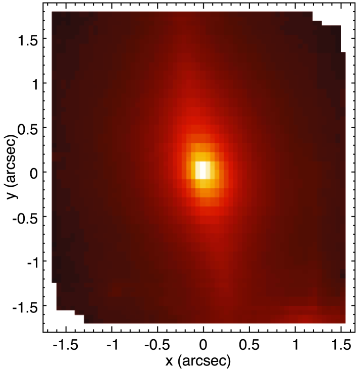
Figure 1: SINFONI image of NGC 4486a.

The SINFONI data reduction package spred (Schreiber et al., 2004; Abuter et al., 2006) was used to reduce the data. It includes all common reduction steps necessary for near-infrared data plus routines to reconstruct the three-dimensional data cubes. After subtracting the sky frames from the object frames, the data were flatfielded, corrected for bad pixels, for distortion and wavelength calibrated using a Ne/Ar lamp frame. The wavelength calibration was corrected using night-sky lines if necessary. Then the three-dimensional data cubes were reconstructed and corrected for atmospheric absorption using the B9.5V star Hip 059503. As a final step all data cubes were averaged together to produce the final data cube. Fig. 1 shows the resulting SINFONI image (collapsed cube) of NGC 4486a. The data of the telluric and the PSF stars were reduced likewise.

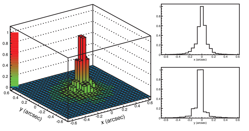
Figure 2: Left: The two-dimensional PSF. Right: x- and y-profiles of the PSF.

As PSF we take the combined and normalised image of the PSF star exposures (see Fig. 2). Its core can be reasonably well fitted by a Gaussian profile with a FWHM of $\sim 100$ mas (7.7 pc). The diameter of the sphere of influence of the black hole can be roughly estimated to $130$ mas using the $M_{\bullet}$-$\sigma$ relation of Tremaine et al. (2002) and is therefore resolved.

3 Kinematics

The kinematic information was extracted using the maximum penalised likelihood (MPL) technique of Gebhardt et al. (2000a), which obtains non-parametric line-of-sight velocity distributions (LOSVDs). As kinematic template stars we use six K0 to M0 stars which were observed during commissioning and our GTO observations in 2005 with SINFONI using the same configuration as for NGC 4486a. Both galaxy and template spectra were continuum-normalised. An initial binned velocity profile is convolved with a linear combination of the template spectra and the residuals of the resulting spectrum to the observed galaxy spectrum are calculated. The velocity profile is then changed successively and the weights of the templates are adjusted in order to optimise the fit to the observed spectrum by minimizing the function $\chi^{2}_{\mathrm{p}}=\chi^{2}+\alpha\mathcal{P}$, where $\alpha$ is the smoothing parameter that determines the level of regularisation, and the penalty function $\mathcal{P}$ is the integral of the square of the second derivative of the LOSVD. We fitted only the first two band heads CO2–0 and CO3–1. The higher-order band heads are strongly disturbed by residual atmospheric features. At wavelength $\lambda<2.29~{}\mathrm{\mu}$m the absorption lines are weak and cannot be fitted very well by the templates.

The uncertainties on the velocity profiles were estimated using Monte Carlo simulations (Gebhardt et al., 2000a). A galaxy spectrum is created by convolving the template spectrum with the measured LOSVD. Then 100 realisations of that initial galaxy spectrum are created by adding appropriate Gaussian noise. The LOSVDs of each realisation are determined and used to specify the confidence intervals.

In order to test the performance of the method on our SINFONI data and to find the best fitting parameters we performed Monte Carlo simulations on a large set of model galaxy spectra. These were created from stellar template spectra by convolving them with both Gaussian and non-Gaussian LOSVDs and by adding different amounts of noise. We found that the reconstructed LOSVDs resemble the input LOSVDs very well if the smoothing parameter $\alpha$ is chosen adequately (Merritt, 1997; Joseph et al., 2001). The best choice of $\alpha$ solely depends on the signal-to-noise ratio (S/N) of the data. To maximize the S/N of the data a binning scheme with 11 radial and 5 angular bins per quadrant, similar to that used in Gebhardt et al. (2003), was chosen. The centres of the angular bins are at latitudes $\vartheta=5.8^{\circ}$, $17.6^{\circ}$, $30.2^{\circ}$, $45.0^{\circ}$ and $71.6^{\circ}$ from the major to the minor axis. The bins are not overlapping, but spatial resolution elements at the border between bins may be divided into parts where each part is counted to a different bin. The spectra within each bin were averaged with weigths according to their share in the bin. The radial binning scheme ensures that an adequate S/N level comparable to that of the central spectrum (S/N$\approx 40$) is maintained at all radii at the cost of spatial resolution outside the central region.

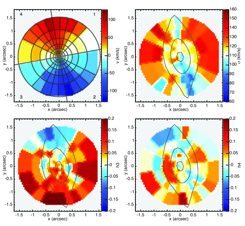
Figure 3: Stellar kinematic fields ($v$, $\sigma$, $h_{3}$, $h_{4}$) of NGC 4486a. The binning scheme and the numbering of the quadrants are overlaid over the velocity map and the isophotes are overlaid over the other maps for comparison.

The resulting two-dimensional kinematics ($v$, $\sigma$, $h_{3}$, $h_{4}$) is presented in Fig. 3. It illustrates the superposition of the kinematics of the two distinct components in NGC 4486a – the disc and the bulge. Whereas the velocity map shows a regular rotation pattern, the cold stellar disc can be clearly distinguished from the surrounding hotter bulge in the velocity dispersion map. The velocity dispersion of the disc is $\approx 20-30$ km s^-1 smaller than that of the bulge. Asymmetric and symmetric deviations from a Gaussian velocity profile are quantified by the higher-order Gauss-Hermite coefficients $h_{3}$ and $h_{4}$ (Gerhard, 1993; van der Marel & Franx, 1993). Fig. 4 shows the kinematic profiles of NGC 4486a along the major axis at angles $\theta=+5.8^{\circ}$ and $\theta=-5.8^{\circ}$. The $+5.8^{\circ}$-profile agrees very well with the adjacent $-5.8^{\circ}$-profile within the error bars. When comparing the profiles at negative radii with the profiles at positive radii slight asymmetries can be seen (especially in $\sigma$), but as the errors are relatively large, deviations from axisymmetry are small.

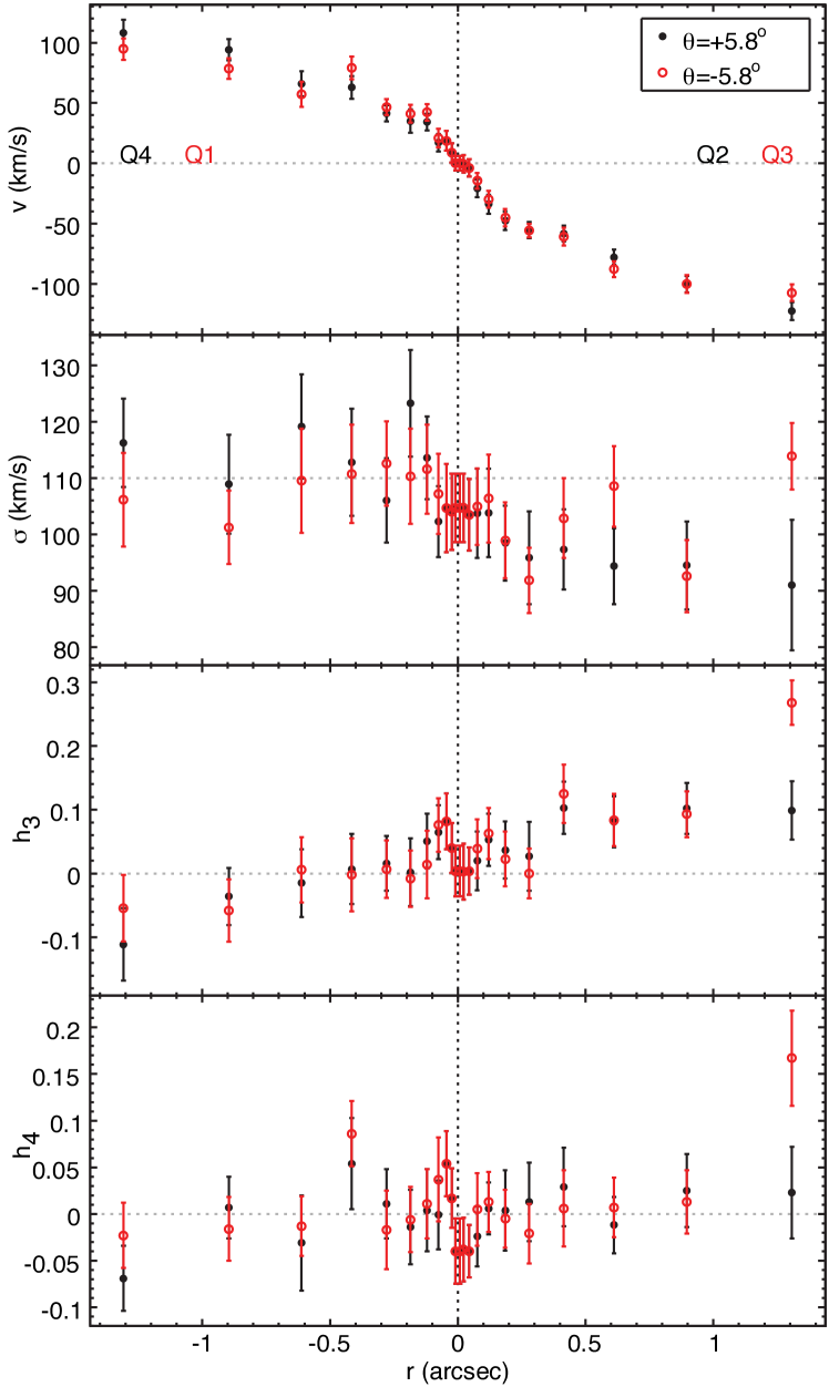
Figure 4: Stellar kinematic profiles ($v$, $\sigma$, $h_{3}$, $h_{4}$) of NGC 4486a along $\theta=\pm 5.8^{\circ}$ of the major axis. The corresponding quadrants crossed by the profiles are marked for easy identification in Fig. 3.

The star at $2.5\arcsec$ from the centre, which heavily dilutes optical spectra of NGC 4486a taken without AO, does not have any significant effect on the kinematics derived here. Quadrant $2$ is affected most, as it is located in the direction of the star. The fraction of inshining light from the star is only about 13% at $0.7\arcsec$ from the centre of the galaxy in the direction of the star (the outermost point covered by the exposures of the PSF star) due to the narrow PSF. In addition the spectrum of the star shows neither the strong CO absorption nor other spectral features in that wavelength region.

4 Imaging

To derive the black hole mass in NGC 4486a, it is essential to determine the gravitational potential made up by the stellar component by deprojecting the surface brightness distribution. As NGC 4486a consists both kinematically and photometrically of two components with possibly different mass-to-light ratios $\Upsilon$, we deproject bulge and disc separately.

To decompose the two components, we considered the HST images in the broad-band F850LP filter, with 2 ACS/WFC pointings of 560 seconds exposure each. The two dithers have no shift in spatial coordinates. The data were reduced by the ST-ECF On-The-Fly Recalibration system, see http://archive.eso.org/archive/hst for detailed information.

Moreover, we use the galfit package (Peng et al., 2002) to fit PSF convolved analytic profiles to the two-dimensional surface brightness of the galaxy. The code determines the best fit by comparing the convolved models with the science data using a Levenberg-Marquardt downhill gradient algorithm to minimize the $\chi^{2}$ of the fit. The saturated star close to the galaxy centre has been masked out from the modelling. The observing strategy, i.e. the adopted no spatial shift between the two dithers, has allowed us to obtain a careful description of the PSF by using the TinyTim code.

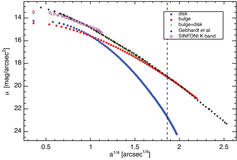
Figure 5: Surface brightness profile for NGC 4486a. At radii left of the dashed line we used the decomposed bulge and disc profiles for the deprojection, right of the dashed line we used the profile of Gebhardt et al. (in prep.) (scaled to ACS $z$-band).

We modelled the galaxy light with a double Sérsic (1968) model with indices $n=2.19$ for the bulge and $n=1.67$ for the disc. In Fig. 5 we show the surface brightness profiles of bulge, disc, bulge+disc, and for comparison the SINFONI surface brightness profile and the un-decomposed profile of Gebhardt et al. (in prep.), which was derived from HST and CFHT imaging in several bands. This profile agrees very well with our combined profile and we use it, scaled to match our profile, at radii $>11.5\arcsec$ where the bulge strongly dominates.

Bulge and disc were then deprojected separately using the program of Magorrian (1999) under the assumption that both components are edge-on and axisymmetric. The stellar mass density then can be modelled as in Davies et al. (2006) via $\rho_{\mathrm{*}}=\Upsilon_{\mathrm{bulge}}\cdot\nu_{\mathrm{bulge}}+\Upsilon_{\mathrm{disc}}\cdot\nu_{\mathrm{disc}}$, where $\nu$ is the luminosity density obtained from the deprojection and the ACS $z$-band mass-to-light ratio $\Upsilon$ is assumed to be constant with radius for both components.

5 Schwarzschild Modelling

The mass of the black hole in NGC 4486a was determined based on the Schwarzschild (1979) orbit superposition technique, using the code of Gebhardt et al. (2000a, 2003) in the version of Thomas et al. (2004). It comprises the usual steps: (1) Calculation of a potential with a trial black hole of mass $M_{\bullet}$ and a stellar mass density $\rho_{\mathrm{*}}$. (2) A representative set of orbits is run in this potential and an orbit superposition that best matches the observational constraints is constructed. (3) Repetition of the first two steps with different values for $\Upsilon_{\mathrm{bulge}}$, $\Upsilon_{\mathrm{disc}}$ and $M_{\bullet}$ until the eligible parameter space is systematically sampled. The best-fitting parameters then follow from a $\chi^{2}$-analysis.

The models are calculated on the grid with 11 radial and 5 angular bins per quadrant as described above (cf. Fig. 3).

Our orbit libraries contain $2\times 7000$ orbits. The luminosity density is a boundary condition and hence exactly reproduced. The $11\times 5$ LOSVDs are binned into $17$ velocity bins each and then fitted directly, not the parametrized moments. We limit the parameter space for the values of $\Upsilon$ by considering the population synthesis model of Maraston (1998, 2005), which gives us $\Upsilon\la 5$ for the $z$-band.

Special care was taken when implementing the PSF. Due to its special shape with the narrow core and the broad wings (cf. Fig. 2) the PSF was not fitted, rather the two-dimensional image of the star was directly used for convolving our models.

Table 1: Results obtained for the four quadrants separately with a global mass-to-light ratio (90% C.L.). The numbering of the quadrants can be inferred from Fig. 3.

Quadrant	$M_{\bullet}$ ($10^{7}$ M⊙)	$\Upsilon$
1	$4.0^{+0.7}_{-2.4}$	$3.4^{+0.6}_{-0.6}$
2	$1.0^{+1.1}_{-0.2}$	$3.6^{+0.2}_{-0.5}$
3	$1.0^{+0.5}_{-0.5}$	$3.8^{+0.6}_{-0.1}$
4	$1.5^{+1.0}_{-1.0}$	$4.4^{+0.3}_{-0.9}$
$1-4$ averaged	$1.25^{+0.3}_{-0.3}$	$4.0^{+0.1}_{-0.4}$

6 Results

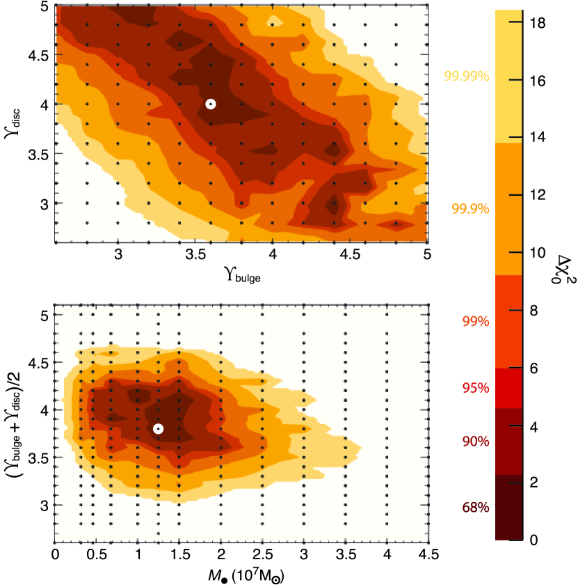
Figure 6: $\Delta\chi_{0}^{2}=\chi^{2}-\chi_{\mathrm{min}}^{2}$ as a function of (top) $\Upsilon_{\mathrm{bulge}}$ and $\Upsilon_{\mathrm{disc}}$, minimized over $M_{\bullet}$; (bottom) $M_{\bullet}$ and $\left(\Upsilon_{\mathrm{bulge}}+\Upsilon_{\mathrm{disc}}\right)/2$. The black points are the models we calculated and the coloured regions are the (unsmoothed) confidence intervals for two degrees of freedom. The best-fitting model is marked with a white circle.

A big advantage of integral-field data compared to longslit data is that we can check the assumption of axisymmetry by comparing the kinematics of the four quadrants and quantify the effect of possible deviations by modelling each quadrant separately. We do not find major differences in the kinematics of the four quadrants (cf. Figs. 3, 4). As it takes a large amount of computing time to calculate all models with different mass-to-light ratios for bulge and disc for each quadrant, we used the same $\Upsilon$ for bulge and disc for the comparison of the quadrants. In Table 1 the resulting values for $M_{\bullet}$ and $\Upsilon$ are listed. They show that the four quadrants agree reasonably well with each other. The only systematically deviant point is the $M_{\bullet}$ determination in the first quadrant that however has a large error and therefore is compatible within the 90% C.L. with the other three quadrants. Therefore we symmetrised the LOSVDs by taking for each bin the weight-averaged LOSVDs of the four quadrants and the corresponding errors. The results of modelling these averaged LOSVDs are shown in Fig. 6, where $\Delta\chi_{0}^{2}=\chi^{2}-\chi_{\mathrm{min}}^{2}$ is plotted as a function of $\left(\Upsilon_{\mathrm{bulge}}+\Upsilon_{\mathrm{disc}}\right)/2$ and $M_{\bullet}$ with error contours for two degrees of freedom. $\Upsilon_{\mathrm{bulge}}$ and $\Upsilon_{\mathrm{disc}}$ anticorrelate such that their sum is approximately constant, as shown in the upper part of Fig. 6. A black hole mass of $(1.25^{+0.75}_{-0.79})\times 10^{7}~{}\mathrm{M_{\sun}}$ (90% C.L.) can be fitted with $\Upsilon_{\mathrm{disc}}\approx 2.8\dots 5.2$ and $\Upsilon_{\mathrm{bulge}}\approx 2.8\dots 4.8$. This result agrees within 90% confidence limit with the results of all quadrants shown in Table 1. The best-fitting model, obtained with minimal regularisation, is marked with a white circle and has a black hole mass $M_{\bullet}=1.25\times 10^{7}\mathrm{M_{\sun}}$ and mass-to-light ratios $\Upsilon_{\mathrm{disc}}=4.0$ and $\Upsilon_{\mathrm{bulge}}=3.6$. The difference in $\chi^{2}$ to the best-fitting model without black hole is $24.14$ which corresponds to $4.5\sigma$. The total $\chi^{2}$ values for the models are around $300$. Together with the number of observables ($11$ radial bins $\times$ $5$ angular bins $\times$ $17$ velocity bins) this gives a reduced $\chi^{2}$ of $\approx 0.3$. Note, however, that the number of observables is in reality smaller due to the smoothing (Gebhardt et al., 2000a).

The dynamical mass-to-light ratios of disc and bulge agree with an old and metal-rich stellar population (Maraston, 1998, 2005). $\Upsilon_{\mathrm{disc}}$ tends to be larger than $\Upsilon_{\mathrm{bulge}}$ which is probably due to the presence of dust in the disc. To estimate the effect of the dust on the mass-to-light ratio of the disc we are using the model of Pierini et al. (2004). For the HST-F850LP filter and an assumed typical optical depth $\tau\la 0.5$ we obtain an attenuation of $A_{\lambda}\la 0.36$ mag. This translates the best-fitting $\Upsilon_{\mathrm{disc}}=4.0$ to a significantly smaller dust-corrected value of $\ga 2.9$. Following the models of Maraston (1998, 2005) this is in good agreement with an estimated $\ga 2$ Gyr younger disc (Kormendy et al., 2005).

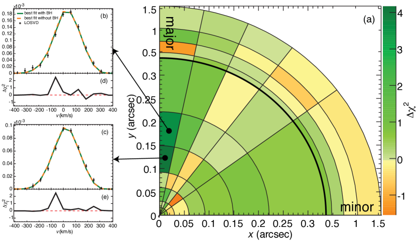
Figure 7: (a) $\chi^{2}$ difference between the best-fitting model without black hole and the best-fitting model with black hole ($\Delta\chi^{2}=\sum_{i}{\Delta\chi_{i}^{2}}=\sum_{i=1}^{17}{\left(\chi^{2}_{i,\mathrm{noBH}}-\chi^{2}_{i,\mathrm{BH}}\right)}$ over all 17 velocity bins) for all LOSVDs of the averaged quadrant. Bins where the model with black hole fits the LOSVD better are plotted in green, the others in orange. The part outside $\approx 2.5$ spheres of influence is plotted with a different scale than the inner part, since in the outer region the dynamical effect of the black hole (and therefore the difference between the two models) is negligible. (b,c) For the radii with the largest positive $\chi^{2}$ difference in (a) the LOSVD (open circles with error bars, normalised as in Gebhardt et al. 2000a) and both fits (with black hole, full green line, and without black hole, dashed orange line) are shown with the corresponding $\Delta\chi_{i}^{2}$ plotted below (d,e).

The significance of the result is illustrated in Fig. 7. It shows the $\chi^{2}$ difference between the best-fitting model without black hole and the best-fitting model with black hole ($\Delta\chi^{2}=\sum_{i=1}^{17}{\left(\chi^{2}_{i,\mathrm{noBH}}-\chi^{2}_{i,\mathrm{BH}}\right)}$ over all 17 velocity bins) for all LOSVDs of the averaged quadrant. The part outside $\approx 2.5$ spheres of influence, where the dynamical effect of the black hole is negligible, is displayed in a compressed way in order to emphasize the important inner part. For $75\%$ of all bins the model with black hole produces a fit to the LOSVD better than the model without black hole. The signature of the black hole is imprinted mainly along the major axis, where the largest positive $\Delta\chi^{2}$ are found at radii $r\approx 0.09\arcsec\dots 0.22\arcsec$. At radii $r\la 0.09\arcsec$ the differences between both models are smaller due to the effect of the PSF. For the radii with the largest $\Delta\chi^{2}$ along the major axis the LOSVD and the fits with and without black hole are shown in the left part of Fig. 7 together with the corresponding $\Delta\chi^{2}_{i}$ as a function of the line-of-sight velocity. The differences between the two fits are relatively small in absolute terms. However, the model without black hole has more stars on the low-velocity wing at a $\sim 1.5\sigma$ level, failing to match fully the measured slightly higher mean velocity of the galaxy. Future observations with a higher spatial resolution should be able to probe this difference more clearly.

The total stellar mass within $1$ sphere of influence, where the imprint of the black hole is strongest, is $M_{*}=9.84\times 10^{6}~{}\mathrm{M_{\odot}}$. If the additional mass of $M_{\bullet}=1.25\times 10^{7}~{}\mathrm{M_{\odot}}$ was solely composed of stars, this would increase the mass-to-light ratio to $\Upsilon_{\mathrm{disc}}\approx 9.1$ ($6.6$ if we take into account the dust-absorption), a region which is excluded by stellar population models or at least requires unrealistic high stellar ages.

The models with black hole become tangentially anisotropic in the centre, while the models without black hole are close to isotropic.

Our result is in good agreement with the prediction of the $M_{\bullet}$-$\sigma$ relation ($1.26^{+0.49}_{-0.35}\times 10^{7}~{}\mathrm{M_{\odot}}$ using the result of Tremaine et al. 2002) and strengthens it in the low-$\sigma$ regime ($\la 120$ km s^-1), where, besides several upper limits, up to now only three black hole masses were measured with stellar kinematics (Milky Way, Schödel et al. 2002; M32, Verolme et al. 2002; NGC 7457, Gebhardt et al. 2003).

NGC 4486a is only the first object in our sample of low-mass galaxies under investigation. The laser guide star, which is presently being installed at the VLT UT4, makes observations of a large number of appropriate galaxies now possible. Therefore we plan to further explore this region of the $M_{\bullet}$-$\sigma$ relation by observing more galaxies with velocity dispersions between the resolution limit of SINFONI ($\sim 30$ km s^-1) and $\sim 120$ km s^-1.

References

- Abuter et al. (2006) Abuter R., Schreiber J., Eisenhauer F., Ott T., Horrobin M., Gillessen S., 2006, New Astronomy Review, 50, 398
- Bender & Kormendy (2003) Bender R., Kormendy J., 2003, in Shaver P., Dilella L., Giménez A., eds, Astronomy, Cosmology and Fundamental Physics Supermassive black holes in galaxy centers. Springer Verlag, p. 262
- Bonnet et al. (2003) Bonnet H., et al., 2003, in Wizinowich P., Bonaccini D., eds, Proc. SPIE Vol. 4839, Implementation of MACAO for SINFONI at the VLT, in NGS and LGS modes. pp 329–343
- Bonnet et al. (2004) Bonnet H., et al., 2004, ESO Messenger, 117, 17
- Burkert & Silk (2001) Burkert A., Silk J., 2001, ApJL, 554, L151
- Davies et al. (2006) Davies R. I., et al., 2006, ApJ, 646, 754
- Eisenhauer et al. (2003a) Eisenhauer F., et al., 2003a, in Iye M., Moorwood A., eds, Instrument Design and Performance for Optical/Infrared Ground-based Telescopes Vol. 4841 of Proc. SPIE, SINFONI—Integral field spectroscopy at 50 milli-arcsecond resolution with the ESO VLT. pp 1548–1561
- Eisenhauer et al. (2003b) Eisenhauer F., et al., 2003b, ESO Messenger, 113, 17
- Ferrarese & Merritt (2000) Ferrarese L., Merritt D., 2000, ApJ, 539, L9
- Gebhardt et al. (2000a) Gebhardt K., et al., 2000a, AJ, 119, 1157
- Gebhardt et al. (2000b) Gebhardt K., et al., 2000b, ApJ, 539, L13
- Gebhardt et al. (2001) Gebhardt K., et al., 2001, AJ, 122, 2469
- Gebhardt et al. (2003) Gebhardt K., et al., 2003, ApJ, 583, 92
- Gerhard (1993) Gerhard O., 1993, MNRAS, 265, 213
- Haehnelt & Kauffmann (2000) Haehnelt M. G., Kauffmann G., 2000, MNRAS, 318, L35
- Joseph et al. (2001) Joseph C. L., et al., 2001, ApJ, 550, 668
- Kormendy et al. (2005) Kormendy J., Gebhardt K., Fisher D., Drory N., Macchetto F. D., Sparks W., 2005, AJ, 129, 2636
- Kormendy & Richstone (1995) Kormendy J., Richstone D., 1995, ARAA, 33, 581
- Magorrian (1999) Magorrian J., 1999, MNRAS, 302, 530
- Maraston (1998) Maraston C., 1998, MNRAS, 300, 872
- Maraston (2005) Maraston C., 2005, MNRAS, 362, 799
- Merritt (1997) Merritt D., 1997, AJ, 114, 228
- Peng et al. (2002) Peng C. Y., Ho L. C., Impey C. D., Rix H.-W., 2002, AJ, 124, 266
- Pierini et al. (2004) Pierini D., Gordon K. D., Witt A. N., Madsen G. J., 2004, ApJ, 617, 1022
- Richstone et al. (1998) Richstone D., et al., 1998, Nat, 395, A14
- Schödel et al. (2002) Schödel R., et al., 2002, Nat, 419, 694
- Schreiber et al. (2004) Schreiber J., Thatte N., Eisenhauer F., Tecza M., Abuter R., Horrobin M., 2004, in Ochsenbein F., Allen M., Egret D., eds, ASP Conf. Proc. Vol. 314, Data reduction software for the VLT Integral Field Spectrometer SPIFFI. p. 380
- Schwarzschild (1979) Schwarzschild M., 1979, ApJ, 232, 236
- Sérsic (1968) Sérsic J. L., 1968, Atlas de galaxias australes. Cordoba, Argentina: Observatorio Astronomico
- Silk & Rees (1998) Silk J., Rees M. J., 1998, A&A, 331, L1
- Thomas et al. (2004) Thomas J., Saglia R., Bender R., Thomas D., Gebhardt K., Magorrian J., Richstone D., 2004, MNRAS, 353, 391
- Tremaine et al. (2002) Tremaine S., et al., 2002, ApJ, 574, 740
- Valluri et al. (2005) Valluri M., Ferrarese L., Merritt D., Joseph C. L., 2005, ApJ, 628, 137
- van der Marel & Franx (1993) van der Marel R., Franx M., 1993, ApJ, 407, 525
- Verolme et al. (2002) Verolme E. K., et al., 2002, MNRAS, 335, 517