Separation of the visible and dark matter in the Einstein ring LBG J213512.73$-$010143

Abstract

We model the mass distribution in the recently discovered Einstein ring LBG J213512.73-010143 (the ‘Cosmic Eye’) using archival Hubble Space Telescope imaging. We reconstruct the mass density profile of the $z=0.73$ lens and the surface brightness distribution of the $z=3.07$ source and find that the observed ring is best fit with a dual-component lens model consisting of a baryonic Sersic component nested within a dark matter halo. The dark matter halo has an inner slope of $1.42^{+0.24}_{-0.22}$, consistent with CDM simulations after allowing for baryon contraction. The baryonic component has a mass-to-light ratio of $1.71^{+0.28}_{-0.38}$ M_⊙/L_B⊙ which when evolved to the present day is in agreement with local ellipticals. Within the Einstein radius of $0.77^{\prime\prime}$ (5.6 kpc), the baryons account for $(46\pm 11)$% of the total lens mass. External shear from a nearby foreground cluster is accurately predicted by the model. The reconstructed surface brightness distribution in the source plane clearly shows two peaks. Through a generalisation of our lens inversion method, we conclude that the redshifts of both peaks are consistent with each other, suggesting that we are seeing structure within a single galaxy.

1 Introduction

The measurement of galaxy mass profiles has proven a powerful observational probe for testing models of structure formation. In recent years, the slope of the inner mass profile has become a subject of much contention with the results of cold dark matter (CDM) simulations being discrepant with observations. At the present time, this discrepancy persists.

Navarro, Frenk & White (1996) first proposed an analytic approximation to describe the mass density profiles of halos in their CDM simulations. At a radius much smaller than a particular scale radius, the mass density of this so called ‘NFW’ profile scales as $\rho(r)\propto r^{-1}$. Later simulations by Moore et al. (1998, 1999) indicated a steeper inner slope. This gave rise to the ‘generalised NFW’ (gNFW) profile which at radii smaller than the scale radius follows $\rho(r)\propto r^{-\alpha}$ with values of $\alpha$ around 1.4 to 1.5. The most recent simulations boasting a significantly higher resolution now converge on a slope somewhere in the range $1.0\mathbin{\lower 3.0pt\hbox{$\hbox to0.0pt{\raise 5.0pt\hbox{$\char 60\relax$}\hss}\mathchar 29208\relax$}}\alpha\mathbin{\lower 3.0pt\hbox{$\hbox to0.0pt{\raise 5.0pt\hbox{$\char 60\relax$}\hss}\mathchar 29208\relax$}}1.2$ (Navarro et al., 2004; Diemand et al., 2005).

These results appear to strongly disagree with measurements of the inner slope from dynamical studies. Several groups measuring rotation curves of low surface brightness galaxies (LSBs; these are believed to have a high dark matter fraction and therefore be minimally affected by baryons) find a range of slopes; $0\mathbin{\lower 3.0pt\hbox{$\hbox to0.0pt{\raise 5.0pt\hbox{$\char 60\relax$}\hss}\mathchar 29208\relax$}}\alpha\mathbin{\lower 3.0pt\hbox{$\hbox to0.0pt{\raise 5.0pt\hbox{$\char 60\relax$}\hss}\mathchar 29208\relax$}}1$ (de Blok et al., 2001; de Blok & Bosma, 2002; Swaters et al., 2003; Spekkens & Giovanelli, 2005). Hayashi et al. (2004) purported that this discrepancy could be reconciled by directly comparing against rotation curves of simulated halos. However, this was strongly rejected by de Blok (2005) who found that only one quarter of the 51 galaxies in the study of Hayashi et al. (2004) were consistent with CDM. In the latest episode of this ongoing debate, Hayashi & Navarro (2006) claim that non-circular motions in simulated CDM halos arising from a triaxial potential can explain the range of measured rotation curves seen in LSBs. Clearly dynamical measurements, whilst potentially very powerful, have many complexities preventing a straight-forward interpretation.

Gravitational lensing has for some time now provided an attractive alternative means of measuring mass profiles without the difficulties associated with dynamical techniques. Primarily, this is motivated by the simple fact that the deflection angle of a photon passing a massive object is independent of the dynamical state of the mass within the object. Strong lensing systems with multiple images of a background source can constrain the radial profile of the projected mass density of the lens by searching for the best fit to the observed image positions (for example, see the review by Schneider, Kochanek & Wambsganss, 2006). This technique was enhanced by Sand, Treu & Ellis (2002) to incorporate extra constraints from the observed velocity dispersion profile of the lens and has since been applied to a number of systems (Treu & Koopmans, 2002; Koopmans & Treu, 2003; Sand et al., 2004).

Dye & Warren (2005, hereafter DW05) showed how Einstein ring systems, i.e., strong lens systems where an extended source is imaged into a complete or near-complete ring, can place stronger constraints on the mass profile of the lens than systems with multiple point-like images. This work used the semi-linear method of Warren & Dye (2003) which has also been used by several other studies to date (Treu & Koopmans, 2004; Treu et al., 2006; Koopmans et al., 2006). A Bayesian version of the semi-linear method was developed by Suyu et al. (2006) and later enhanced by Barnabè & Koopmans (2007) with the inclusion of linear constraints from stellar velocity moments.

In this paper, we follow the procedure of DW05. We apply the semi-linear method to reconstruct the lens mass profile and source surface brightness image of the extraordinary Einstein ring system LBG J2135-0102 recently discovered by Smail et al. (2007, see also Coppin et al. 2007). Due to the lens amplification, this system is of particular interest as it represents one of the brightest examples of Lyman break galaxies known.

We compare the fit given by five different lens models. With our most general model which comprises a gNFW halo that hosts a mass component following the lens galaxy light, we separate the baryonic and dark matter contributions to the projected lens mass within the Einstein radius. We also describe a simple extension of the semi-linear method enabling reconstruction of sources in multiple planes at different redshifts. Our analysis adds to the growing list of Einstein ring systems that are now beginning to provide strong constraints on CDM simulations.

The layout of this paper is as follows. In the following section we briefly describe the data. Section 3 outlines the semi-linear method and our lens models. We present the results of our source and lens reconstruction in Section 4. Finally, we conclude with a summary and discussion in Section 5. Throughout this paper, we assume the following cosmological parameters; ${\rm H}_{0}=70\,{\rm km\,s}^{-1}\,{\rm Mpc}^{-1}$, $\Omega_{m}=0.3$, $\Omega_{\Lambda}=0.7$.

2 Data

The image data were acquired as part of the Snapshot programme GO #10491 (PI: H. Ebeling) on May 8th 2006 using the Hubble Space Telescope (HST) Advanced Camera for Surveys (ACS). Imaging of the Einstein ring itself was completely serendipitous, the intended target being the cluster MACS J2135.2-0102 lying approximately $75^{\prime\prime}$ away to the south. The top panel of Figure 1 shows a section of the reduced ACS image with the Einstein ring and lens galaxy just to the left of centre. The cluster centre lies at $24^{\circ}$ in a counter-clockwise direction measured from the +ve $x$-axis. The nearby galaxies labeled A, B and C are likely cluster members. We consider the perturbative effect from these nearby galaxies and the large scale shear from the cluster itself on the lens solution in Section 4.1.

The image is a stack of three dithered 400s exposures taken with the ACS Wide Field Camera (WFC) in the F606W filter. The stack was produced using the STScI MULTIDRIZZLE package (V.2.7) thereby correcting for the geometric shear introduced by the WFC and giving a resulting pixel scale of $0.05^{\prime\prime}$. The reader is referred to Smail et al. (2007) for more details.

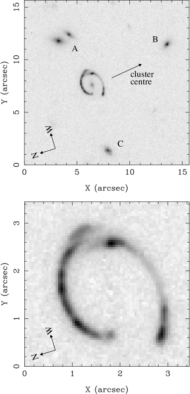
Figure 1: The ACS Wide Field Camera data observed in F606W. North lies at an angle of $197.4^{\circ}$ measured counter-clockwise from the positive $x$-axis. Top: The Einstein ring and lens galaxy showing the nearby likely cluster members labeled A, B and C. The cluster MACS J2135.2-0102 lies $75^{\prime\prime}$ away to the south as indicated. Bottom: The ring after subtraction of the lens galaxy satisfactorily fit with a Sersic profile.

Keck spectroscopy taken on June 30th 2006 and July 24th 2006 unambiguously identifies the lensed source as a Lyman break galaxy lying at a redshift of $z=3.07$. Similarly, the lens galaxy spectrum exhibits several strong absorption and emission features placing it at a redshift of $z=0.73$. The total magnitude of the lens galaxy in the F606W filter is $R_{F606W}=22.34\pm 0.15$ (Smail et al., 2007). In addition to the ACS imaging data, Smail et al. (2007) obtained a $K^{\prime}$ image using the Near Infra-Red Camera at Keck II on July 4th 2006. The ($R_{F606W}-K^{\prime}$)=2.8 colour of the lens and the spectral continuum is consistent with that of an early type spiral or S0 galaxy.

Before reconstructing the source surface brightness distribution, any contribution of flux from the lens galaxy to the ring flux must be removed. Although the lens contribution in this case is unlikely to be of concern, we carried out this exercise anyway to establish the visible morphology of the lens for our modelling later. An added complication in this case is that the lens galaxy light is sheared by the foreground cluster and this must be accounted for in the lens model (Section 3.3.1). We fitted an elliptical Sersic profile (Sérsic, 1968) of the form

$${\rm L}={\rm L}_{1/2}\exp\{-B(n)[(r/r_{s})^{1/n}-1]\}$$ (1)

to the lens galaxy having first masked out pixels within an elliptical annulus containing the ring (see Figure 3). For the fitting of this profile and for the modelling later, we created a noise map based on the CCD gain, read noise and photon count. The parameters ${\rm L}_{1/2}$, $n$ and $r_{s}$ were allowed to vary in the fit as well as the elongation (i.e., major axis divided by minor axis), $e$, and the orientation (angle in degrees of the major axis to the positive image $x$-axis in a counter-clockwise sense), $\theta$. In the fitting, we convolved each trial surface brightness profile with the WFC point spread function (PSF) modelled by the TinyTim package (Krist & Hook, 2004) for the F606W filter. The best fit was achieved with the parameters listed in Table 1 which give an acceptable $\chi^{2}$.

Parameter	Minimised Value
${\rm L}_{1/2}$	$(3.14\pm 0.25)\times 10^{9}\,{\rm L}_{B\odot}/\Box^{\prime\prime}$
$n$	$2.90\pm 0.12$
$r_{s}$	$0.57^{\prime\prime}\pm 0.09^{\prime\prime}$
$\theta$	$110.1^{\circ}\pm 2.6^{\circ}$
$e$	$1.38\pm 0.07$

Table 1: Parameters of the Sersic profile fit to the lens galaxy. Reading from top to bottom, these are; the surface brightness at the scale radius (${\rm L}_{1/2}$), the Sersic exponent ($n$), the scale radius ($r_{s}$), the orientation of the major axis to the positive image $x$-axis in a counter-clockwise sense ($\theta$) and the elongation, i.e. major axis divided by minor axis ($e$).

We work in terms of the rest-frame $B$ band luminosity in this paper for ease of comparison with other studies. The conversion from F606W flux (approximately rest-frame $U$) to $B$ band luminosity density was made using a k-correction and a colour correction (see Section 3.3). The fitted profile was subtracted from the unmasked image and the result is shown in the lower panel of Figure 1.

3 Method of Analysis

3.1 Semi-linear inversion

For a full description of the semi-linear inversion method, the reader is referred to Warren & Dye (2003) and DW05. We provide a very brief outline here for completeness.

The inversion assumes the source plane and the image plane are pixelised. The manner in which the source plane is pixelised is not restricted, allowing the ‘adaptive gridding’ described in DW05 whereby smaller pixels are concentrated in regions where there are stronger constraints (see next section).

For a given lens model parameterisation, a PSF-smeared image is computed for every source pixel. All images are created using unit surface brightness source pixels. The problem of finding the factor required to scale each image such that their co-addition best fits the observed image is a linear one. These scale factors are the best fit surface brightnesses of the source pixels for the given lens model. The solution is written as

$$\underline{s}=({\rm\underline{F}}+\lambda{\rm\underline{H}})^{-1}\underline{c}\,,$$ (2)

where the square matrix ${\rm\underline{F}}$ and the vector ${\rm\underline{c}}$ have the elements

$${\rm F}_{ik}=\sum_{j}f_{ij}f_{kj}/\sigma_{j}^{2}\,,\,\,\,c_{i}=\sum_{j}f_{ij}d_{j}/\sigma_{j}^{2}$$ (3)

and $\underline{s}$ is a vector containing the best fit source pixel surface brightnesses. Here, $d_{j}$ is the observed flux in image pixel $j$, $\sigma_{j}$ its error and $f_{ij}$ is the flux in pixel $j$ of the image of source pixel $i$ for the current lens model. The solution is regularised by the square regularisation matrix ${\rm\underline{H}}$, scaled by the regularisation weight $\lambda$ (see Press et al., 2001, and Warren & Dye 2003). The standard errors of the reconstructed source pixels are given by the diagonal terms of the covariance matrix which is just:

$$({\rm\underline{F}}+\lambda{\rm\underline{H}})^{-1}\,.$$ (4)

This linear inversion is nested inside an outer loop that varies the non-linear lens model parameters. For each trial set of lens parameters, the image of the reconstructed source is compared to the observed image and the $\chi^{2}$ computed within an elliptical mask containing the ring. The mask is designed to ensure that it includes the image of the entire source plane, with minimal extraneous sky. This means that only significant image pixels are used in the fit, making $\chi^{2}$ more sensitive to the model parameters.

The regularisation scheme is chosen to best suit the reconstructed source surface brightness image. Warren & Dye (2003) showed using simulations that linear regularisation works well for this application. However, as we discuss in the next section, regularisation biases the solution between different lens models and so we set $\lambda=0$ and use an adaptive source grid when searching for the best fit lens parameters.

In DW05, we used a downhill simplex method to find the set of lens parameters that minimises $\chi^{2}$. However, the $\chi^{2}$ surface is pitted with local minima and noisy. Warren & Dye (2003) described how this noise can be reduced by sub-gridding the image pixels when computing the source pixel images. In this work, we therefore divide image pixels into $16\times 16$ sub-pixels. To prevent becoming trapped in local minima, we use a simulated annealing downhill simplex minimisation algorithm. We find that a slow exponentially cooled temperature with a half-life of $\sim 50$ iterations works extremely well in finding the global minimum.

3.1.1 Multiple source planes

As we show in Section 4.2, the reconstructed source surface brightness distribution of LBG J2135-0102 has two distinct peaks. An interesting question to ask is therefore whether these peaks are two separate objects at different redshifts or, given their small angular separation, two flux peaks within the same object. The ring spectra presented in Smail et al. (2007) show no evidence of a different secondary source redshift although the fainter source would be dominated by the brighter and much more highly magnified primary source (see also the discussion of the CO emission from this system in Coppin et al., 2007). We explain here how the semi-linear inversion method can be modified in a simple way to place constraints on this problem.

The inversion described above is completely general in terms of the geometry of each source pixel and the lens model. Qualitatively, this means that each source pixel image can be created assuming a different lens configuration. The practical use of this is not in changing the lens mass profile, but the lens geometry so that different source pixels can be assigned different redshifts. In the case of two source planes, this quantitatively means that the vector $\underline{s}$ in equation (2) holds two groups of source pixels, $s_{1}\rightarrow s_{n}$ and $s_{n+1}\rightarrow s_{n+m}$. The matrices ${\rm\underline{F}}$ and ${\rm\underline{H}}$ and the vector $\underline{c}$ are computed in exactly the same way as described in Warren & Dye (2003), except the lens configuration for the first $n$ pixels uses a different source redshift to that for the remaining $m$ pixels.

In this paper, we carry out the usual reconstruction with a single source plane, then a separate analysis with two source planes. For the second analysis, we define two source planes; plane 1 containing pixels that belong to the brightest and more highly magnified source and plane 2 containing pixels of the fainter source as Figure 3 shows. To investigate whether the redshift of source 2 is consistent with that of source 1, we hold plane 1 fixed at the measured spectroscopic redshift $z=3.07$ and allow the redshift of plane 2 to vary. This introduces an extra non-linear lens model parameter (see Section 3.3). In the minimisation, all lens parameters including this additional parameter are allowed to vary.

3.2 Adaptive source plane grid

We adopt the gridding algorithm of DW05 in the current paper which creates smaller source plane pixels where the magnification is higher. The gridding algorithm starts with a regular mesh of large pixels. For a given lens model, the average magnification $\mu_{i}$ of every source pixel $i$ is computed. Those pixels that meet the criterion $\mu_{i}\,r_{i}\geq s$ are then split into quarters, where $r_{i}$ is the ratio of the area of pixel $i$ to the area of an image pixel and $s$ is the ’splitting factor’. Having finished the initial loop through all pixels, the process is repeated for the sub-pixels, then for the sub-sub-pixels and so on until all pixels satisfy the splitting criterion. The entire procedure (which takes a fraction of a second on a modern desktop computer) is repeated every time the lens model changes.

The splitting factor is set empirically by measuring the improvement in the fit brought about by the splitting for different values of $s$ with a fixed lens model close to the best solution. The splitting factor is successively reduced until no significant improvement is obtained. For our unregularised reconstruction, we find a splitting factor of $s=9$ satisfies this condition. By initialising the adaptive gridding with a source plane of regular $0.1^{\prime\prime}\times 0.1^{\prime\prime}$ pixels, this splitting factor ensures that images of split source pixels do not exceed the Nyquist sampling resolution set by the image PSF (see DW05 for more details on how $s$ is set and how the initial grid size is chosen). This is important since it keeps degeneracies between source pixels to a very low level, thereby allowing the number of degrees of freedom to be accurately determined (see below).

The main advantage of an adaptive grid is that the resolution of the reconstructed source can be enhanced relative to a regular grid without the need for regularisation. Regularisation has the effect of smoothing the reconstructed source light profile, reducing the effective total number of parameters and hence increasing the number of degrees of freedom, by an amount that cannot be satisfactorily quantified. This is especially problematic when comparing different lens models, as a fixed regularisation weight for one model generally does not give the same increase in number of degrees of freedom for another. This problem was noted by Kochanek, Schneider & Wambsganss (2004). Adaptively sized pixels extract maximum information from the lens image without need of regularisation. Therefore, provided the degeneracies between all pairs of source pixels are negligible, the number of degrees of freedom of the fit is a well–defined number. This allows, firstly, unambiguous assessment of whether a given model provides a satisfactory fit to the data and secondly, unbiased comparison of different model fits.

Suyu et al. (2006) and Barnabè & Koopmans (2007) suggest an alternative means of circumventing this problem with a Bayesian approach. They point out that the Bayesian evidence enables different lens models and regularisation weights to be compared in an unbiased way. However, we prefer to adhere to the adaptive grid technique without regularisation since this has the appealing characteristic that the error image of the reconstructed source is much more uniform. To ensure that the number of degrees of freedom we compute in our unregularised solution is accurate, we verify that the degeneracies between all source pixel pairs are negligible by ensuring that all off diagonal terms in the covariance matrix given by equation (4) are negligible.

Although regularisation is not used when quantifying lens model fits, we use it in this paper solely for the aesthetic purpose of obtaining a higher resolution source. In DW05, we used zeroth order regularisation to simplify the implementation. However, this is an over-simplistic type of regularisation since it poorly represents real astronomical sources. A better scheme is linear regularisation where pixels that differ more strongly in surface brightness from their neighbours are penalised more heavily. We implement a form of linear regularisation on the adaptive grid in the current paper by constructing a regularisation matrix that takes the difference between a given pixel $i$ and the sum of all neighbouring pixels $j$ weighted by $w_{ij}=(a_{j}/a_{i})\,N\exp(-y_{ij}^{2}/2\sigma^{2})$. Here, $a$ is the source pixel area, $y_{ij}$ is the separation of the centres of pixels $i$ and $j$ and $N$ is a normalisation constant set such that $\sum_{j,j\neq i}w_{ij}=1$. We set $\sigma=0.05^{\prime\prime}$. As described in DW05, we use a smaller splitting factor when applying regularisation. Figure 3 shows the adaptive grids upon which the regularised and unregularised source is reconstructed.

3.3 Lens model

We compare the fit given by five different parameterisations of the lens mass profile. The most general of these is a dual component model. In this model, one component follows the lens galaxy light (the baryons) and the other, a gNFW profile represents the dark matter halo. The remaining four single component models are special cases of the dual component model; 1) a singular isothermal ellipsoid (SIE), 2) a gNFW profile, 3) a power-law model, 4) a mass-to-light (M/L) model where the mass follows the lens galaxy light.

The dual component model is that used by DW05. For the baryonic component, only the $B$ band M/L ratio, $\Psi$, is allowed to vary during the minimisation. Its morphology is fixed by the lens galaxy surface brightness profile that would have been observed in the absence of cluster shear. This is simply a transformation of the Sersic profile fit to the observed surface brightness profile (see Section 3.3.1).

The dark matter halo component is described by an elliptical gNFW profile with a volume mass density given by

$$\rho(r)=\rho_{s}(1+r/r_{0})^{\alpha-3}(r/r_{0})^{-\alpha}.$$ (5)

The halo has seven parameters; the normalisation, $\rho_{s}$, the inner slope $\alpha$, the offset of the halo centre from the baryonic centre, $(\Delta x_{h},\Delta y_{h})$, the scale radius $r_{0}$, the elongation $e_{h}$ (equal to the major:minor axis ratio) and the orientation of the major axis to the positive image $x$-axis in a counter-clockwise sense, $\theta_{h}$. As we discussed in DW05, the scale radius is very weakly constrained in this model, hence we hold it fixed at the value of $r_{0}=3.0^{\prime\prime}$ in accordance with the results of Bullock et al. (2001) for a galaxy with similar total mass and redshift properties to the lens.

We include the effect of the nearby cluster in two ways. Firstly, we incorporate an external shear that is allowed to vary in magnitude, $\gamma$, and direction, $\theta_{\gamma}$ (measured counter-clockwise from the +ve $x$-axis). The cluster convergence must also be accounted for, as this causes magnification of the ring image. We therefore calculate a convergence based on $\gamma$ and $\theta_{\gamma}$ assuming a SIE profile (using a NFW profile for this purpose instead makes little difference to the best fit lens model parameters compared to the size of their errors). Secondly, we model perturbations in the cluster potential from the nearby cluster galaxies. In this case, each galaxy is modelled as a SIE with a mass given by its total integrated light multiplied by a common $B$ band M/L, $\Psi_{cg}$.

In summary, our dual component model has a total of ten free parameters; $\Psi$, $\rho_{s}$, $\alpha$, $(\Delta x_{h},\Delta y_{h})$, $\theta_{h}$, $e_{h}$, $\gamma$ , $\theta_{\gamma}$ and $\Psi_{cg}$. The single component models are obtained by holding various combinations of these parameters fixed. For the gNFW model, we only fix $\Psi=0$ and allow all other parameters, including the cluster parameters ($\gamma$, $\theta_{\gamma}$ and $\Psi_{cg}$) to vary. Similarly, for the power-law and SIE models, the halo scale radius, $r_{0}$, is held at an arbitrarily large value having fixed $\Psi=0$ with the additional constraint $\alpha=2$ for the SIE. The pure M/L model allows only $\Psi$ and the cluster parameters to vary.

The deflection angles of both the Sersic and gNFW profiles must be numerically evaluated. Also, the surface mass density of the gNFW profile must be obtained by numerically integrating along the line of sight. We showed in DW05 how we convert the circular Sersic and gNFW profiles to elliptical profiles.

The surface mass density of the Sersic profile is obtained by multiplying the fitted light profile given in equation (1) by the M/L ratio, $\Psi$. To convert the lens galaxy flux measured in the F606W filter to a $B$ band luminosity, we computed a k-correction and a colour correction using a standard S0 and Sa galaxy template taken from Mannucci et al. (2001). These SEDs are consistent with the $(R-K^{\prime})$ colour measured by Smail et al. (2007) and the observed lens morphology. The k-correction and colour correction for the S0 template are respectively -1.85 mag and 2.03 mag, and for the Sa template, -1.69 mag and 1.97 mag. We take the average k-correction and colour correction and treat the difference in each as a 1$\sigma$ error. Similarly, for the perturbing cluster galaxies, we assumed a standard elliptical spectrum to convert to a $B$ band luminosity. For the cluster redshift of $z=0.33$, the colour correction is 2.06 mag and the k-correction -0.63 mag.

3.3.1 Modelling procedure

Since the nearby foreground cluster shears the light from the lens galaxy as well as the ring image, the morphology of the baryons cannot be simply fixed as the Sersic profile fit to the observed lens galaxy surface brightness (see Section 2). In theory, we could allow the baryonic morphology to vary in the minimisation. However, in practice, the morphology proves very poorly constrained since the baryons have only a small elongation (see Section 4.1) and only contribute approximately one third of the total projected mass inside the Einstein radius (including the cluster convergence).

With this in mind, we adopt the following procedure when fitting the lens with the dual component model and pure M/L model:

• First fit the gNFW, power-law and SIE models to determine the best fit cluster shear.

• Using the average of this best fit shear, compute the elongation and orientation of the Sersic profile that would have been observed in the absence of the cluster.

• Fit the dual component model, fixing the baryon component with the Sersic profile parameterised in Table 1, except with the elongation and orientation computed in step 2.

We compute an error on the elongation and orientation estimated in step 3 by combining the errors from the original Sersic fit, as given in Table 1, and the error on the shear determined in step 1. This resulting uncertainty is incorporated into our modelling using a Monte Carlo simulation which randomly samples the orientation and elongation for 100 minimisations. The final errors we quote combine the spread in minimised model parameters with the formal errors from the fit and additionally include the colour and k-correction error for the M/L.

Having fit each of the five lens models, we repeat the analysis with the best fit model and a second source plane. In this case an additional parameter, $z_{2}$, is introduced for the second source plane redshift.

4 Results

4.1 Lens reconstruction

Table 2 compares the $\chi^{2}$ for the five models. The best fit to the observed ring is given by the dual component model. The pure M/L model is very strongly ruled out. The pure halo, power-law and SIE models give a satisfactory $\chi^{2}$ but perform significantly worse than the dual component model with $\Delta\chi^{2}=17.4$ for six fewer degrees of freedom for the gNFW, $\Delta\chi^{2}=16.2$ for 12 fewer degrees of freedom for the power-law and $\Delta\chi^{2}=22.8$ for the SIE.

Model	$\chi^{2}_{\rm min}$	NDoF	Nsrc	Npar
dual component	1912.6	1896	278	10
SIE	1935.4	1888	289	7
pure gNFW	1930.0	1890	285	9
power-law	1928.8	1884	291	9
pure M/L	2188.4	1920	260	4

Table 2: Comparison of the lens models in terms of $\chi^{2}$ at the minimum. The number of degrees of freedom (NDoF) for each model is given by the number of image pixels in the elliptical annulus ($=2184$ – see Figure 3) minus the sum of the number of source pixels in the adaptive grid (N_src) and the number of parameters in the lens model (N_par).

We fitted the gNFW, power-law and SIE models first to establish the cluster shear (see Section 4.1.1). The normalisation of the SIE model corresponds to a central velocity dispersion of $210\pm 10$ km s^-1, in agreement with the measurement of $\sim 230\pm 30$ km s^-1 from the lens galaxy spectrum (Smail et al., 2007). The slope of the gNFW model is $1.95\pm 0.03$, consistent with the slope of $2.01^{+0.02}_{-0.03}$ averaged over 15 lenses by Koopmans et al. (2006). Similarly, the best fit slope of the power-law model is $2.09\pm 0.04$.

Using the average shear obtained from the gNFW and SIE models, we distorted the Sersic profile fitted to the observed galaxy light to give a resulting elongation of $1.14\pm 0.08$ and orientation $23.2^{\circ}\pm 4.2^{\circ}$. This sheared Sersic profile was then used to fix the morphology of the baryonic component for the pure M/L model and the dual component model.

The best fit parameters of the dual component model are given in Table 3. The baryonic component accounts for $46\pm 11$% of the total lens mass inside the Einstein radius of $0.77^{\prime\prime}$ (5.6 kpc). This excludes the convergence from the cluster and its nearby perturbing galaxies which contribute a total of $\sim 20\%$ of the projected mass inside the Einstein radius. The baryonic fraction is lower than the fraction $64\pm 4$% (18% rms scatter) found by Gavazzi et al. (2007) in averaging over 22 strong lenses, although is within their spread of $40\%-100\%$. The halo alignment is consistent with the baryons, both positionally and in orientation. The elongation of both components is also consistent, although the errors are relatively large, predominantly due to a degeneracy between the halo elongation and the shear. We discuss the cluster shear further in Section 4.1.1.

Parameter	Minimised Value
$\rho_{s}$	$(1.42\pm 0.24)\times 10^{7}\,{\rm M}_{\odot}{\rm kpc}^{-3}$
$\alpha$	$1.42^{+0.24}_{-0.22}$
$\Psi$	$1.71^{+0.28}_{-0.38}$ M⊙/LB⊙
$e_{h}$	$1.12^{+0.09}_{-0.07}$
$(\Delta x_{h},\Delta y_{h})$	$(-0.03^{\prime\prime}\pm 0.03^{\prime\prime},0.06^{\prime\prime}\pm 0.03^{\prime\prime})$
$\theta_{h}$	$20.3^{\circ}\pm 3.5^{\circ}$
$\gamma$	$0.181\pm 0.021$
$\theta_{\gamma}$	$29.6^{\circ}\pm 4.1^{\circ}$
$\Psi_{cg}$	$3.6\pm 1.9$ M⊙/LB⊙

Table 3: Best fit parameters for the dual component model (see Section 3.3). 1$\sigma$ errors are quoted.

Figure 2: One-parameter confidence regions (1, 2, 3 & 4$\sigma$) on the halo inner slope, $\gamma$, and M/L_B⊙ of the baryons, $\Psi$, for the dual component model (see Treu & Koopmans, 2004; Dye & Warren, 2005, for comparison).

In Figure 2, we plot the confidence levels on the fitted inner halo slope and baryonic M/L, having marginalised over all other parameters. The best fit slope is $\alpha=1.42^{+0.24}_{-0.22}$. This is consistent with the value measured by Treu & Koopmans (2004) of $1.3^{+0.2}_{-0.4}$ with their baryons $+$ halo model, averaged over three lenses although slightly higher than the value measured by DW05, $\alpha=0.87^{+0.34}_{-0.27}$ (their 68% CL) for the Einstein ring 0047-2808. The best fit M/L is $1.71^{+0.28}_{-0.38}$ M_⊙/L_B⊙ which compares to the local value for ellipticals measured by Gerhardt et al. (2001) of $7.3\pm 2.1$ M_⊙/L_B⊙. To evolve this local measurement back to the redshift of our lens, we use the findings of Koopmans et al. (2006) that d$\log({\rm M/L}_{B})/$d$z=-0.69\pm 0.08$. This gives a result of M/L${}_{B}=2.3\pm 0.7$ M_⊙/L_B⊙, slightly higher than our measurement but consistent within the errors.

A source of error not included in Figure 2 is the uncertainty on the halo scale radius $r_{0}$. However, the propagation of this uncertainty is small. We find that a 10% change in $r_{0}$ gives rise to a $\sim 1\%$ change in the minimised M/L and a negligible change in the minimised slope. This is exactly the same dependency found by DW05.

Finally, turning to the perturbing cluster galaxies, we find a best fit $B$ band M/L of $\Psi_{cg}=3.6\pm 1.9$ M_⊙/L_B⊙. This is in keeping with local ellipticals as well as ellipticals found in $z\sim 0.3$ clusters (e.g., Natarajan & Springel, 2004). We note that if these cluster members are omitted from the modelling then the best fit elongation of all models (apart from the pure M/L) has to be significantly higher, $e_{h}\simeq 1.4-1.5$ in order to fit the observed ring image. In this case, the fit is not significantly degraded, but contradicts the concordant view that isodensity contours have consistent or smaller elongations than isophotal contours for a given system (e.g., Koopmans et al., 2006).

4.1.1 Cluster shear

The best fit cluster shear predicted by the gNFW, power-law and SIE models was found to be respectively ($\gamma=0.182\pm 0.017$, $\theta_{\gamma}=27.6^{\circ}\pm 3.3^{\circ}$), ($\gamma=0.180\pm 0.018$, $\theta_{\gamma}=28.1^{\circ}\pm 3.4^{\circ}$) and ($\gamma=0.176\pm 0.014$, $\theta_{\gamma}=29.1^{\circ}\pm 2.9^{\circ}$).

As well as being self-consistent, this shear is in agreement with what would be expected from an isothermal cluster mass profile: Firstly, the tangential shear angle $\theta_{\gamma}$ is consistent with the direction of the cluster centre at $24^{\circ}$. Secondly, the magnitude is what would be expected given the cluster proximity as the following approximate calculation demonstrates: The ring lies $\sim 1.8$ times further away from the cluster centre than the outermost (and faintest) arc. Making the reasonable assumption that this arc is an image of a $z\mathbin{\lower 3.0pt\hbox{$\hbox to0.0pt{\raise 5.0pt\hbox{$\char 62\relax$}\hss}\mathchar 29208\relax$}}2$ source and since the deflection angle varies very slowly with redshift beyond $z\sim 2$, this gives a good approximation to the critical radius for a source at infinity. Treating the cluster mass profile as an isothermal sphere gives a predicted shear of $\gamma=0.28$ for a $z\rightarrow\infty$ source at $r=1.8r_{\rm crit}$. However, a source at the lens redshift of $z=0.73$ experiences a shear of 0.63 times less (for our assumed cosmology) resulting in a shear of $\gamma=0.175$.

The average of the shear from the gNFW, power-law SIE models was used to distort the Sersic profile fitted to the observed galaxy light. With this distorted profile, the dual component model gives a best fit cluster shear of $\gamma=0.181\pm 0.021$, $\theta_{\gamma}=29.6^{\circ}\pm 4.1^{\circ}$. The error budget here includes the uncertainty on the distorted Sersic profile. This shear agrees very well with the shear obtained from the gNFW, power-law and SIE models, an indication that the lack of baryons in these models did not bias the shear they predict.

The ability to predict the large scale cluster shear from the small area of sky covered by the ring is quite remarkable. Although the shear is fairly degenerate with the lens elongation, this degeneracy is significantly higher in strong lens systems with only a point-like source, to the extent that measurement of external shear in these systems is impossible. This is a testament to the stronger constraints provided by an extended source.

4.2 Source reconstruction

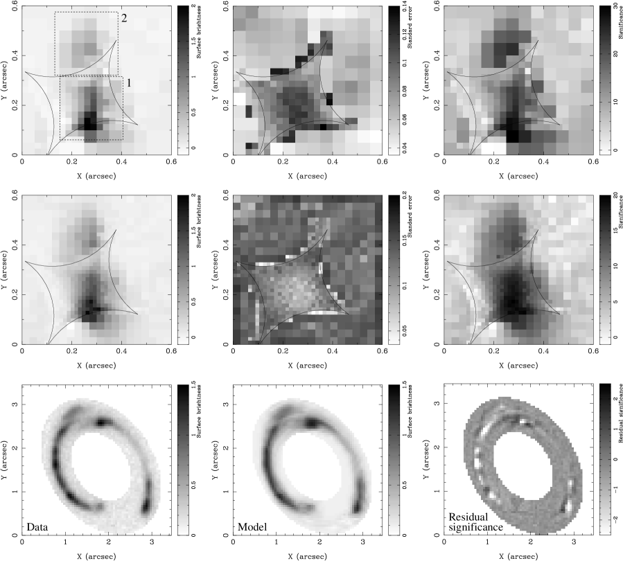
Figure 3: The reconstructed source from the best fit dual component model. Reading from left to right along each row; Top row - the unregularised reconstructed source, the standard errors map for the reconstructed source and the significance map; Middle row - same as top row but for the regularised source; Bottom row - the masked observed ring, the image of the unregularised source and the significance of the residuals. As can be seen, the lens model gives a very good description of the observed ring morphology. The reconstructed source shows two peaks. In the top left panel, the dashed squares delineate the two source planes used in the dual-source reconstruction (labeled 1,2). The source plane caustic is indicated in the top two rows. In the source plane, $0.1^{\prime\prime}$ corresponds to 800pc.

Figure 3 shows the reconstructed source obtained from the best fit dual component model. The top row corresponds to the unregularised solution and the middle row the regularised case. In the bottom row we plot the observed image alongside the image of the unregularised source and the significance of the residuals. The residuals are within $\pm 2.5\sigma$. Considering some of the pixels in the observed image reach a significance of $\sim 40\sigma$, this demonstrates the quality of the fit. Nevertheless, we have investigated the cause of these residuals, i.e., whether they are due to an overly-coarse source pixelisation, the parameterisation of the lens model or the PSF used to smear images of lensed source pixels. The source pixelisation is ruled out by the fact that the residuals are barely changed when we use the image of the regularised source. We also repeated the minimisation with different PSFs, including a PSF extracted from stars in the field, but the best fit was obtained with the TinyTim model PSF (see Section 2). We conclude therefore that the residuals would probably be lessened by a small modification in the parameterisation of the lens model. This would require an exhaustive search through different parameterisations with only a small return and no guarantee of finding a unique solution, hence we leave this for possible future work.

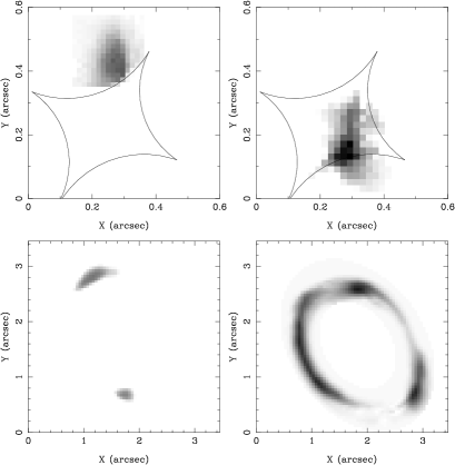
Figure 4: The contribution of each reconstructed source to the observed ring image. The top row shows the two sources and the bottom row their respective images.

The total magnification of the system (i.e., total ring flux divided by total source flux) is $\sim 25$. There are clearly two peaks in the source surface brightness distribution. To demonstrate the contribution each peak makes to the observed Einstein ring image, Figure 4 shows the image of each peak lensed separately with the best fit dual component model. The dominant ring structure is due to the brighter peak mostly contained within the caustic. The fainter peak lying nearer the top of the plane and outside of the caustic is imaged into the westerly and easterly extensions. Although not plotted, the double-peaked nature of the reconstructed source obtained with the other models is reproduced in every case.

4.2.1 Dual source plane analysis

We repeated the minimisation using the dual component model but with two separate source planes as indicated in the top left panel of Figure 3. Source plane 1 containing the brighter source peak was held fixed at the redshift $z=3.07$ but the redshift of source plane 2, $z_{2}$, was allowed to vary in the minimisation.

Our results give a value of $z_{2}=3.13^{+0.73}_{-0.49}$ with an overall fit that is not an improvement on the single source plane case. The remaining minimised parameters of the model differ only negligibly to those in Table 3 for the single source plane case. Although the errors are large, the redshift of the second source peak is consistent with that of the brighter primary peak, suggesting that these are two features within the same galaxy.

5 Summary and Discussion

Out of the five lens models assessed in this work, the Einstein ring LBG J2135-0102 is best fit with our dual component model comprising a gNFW dark matter halo that hosts a baryonic component following the lens galaxy light. Of the remaining four single component models, the gNFW, power-law and SIE models give an acceptable fit but the pure M/L model is very strongly ruled out. Between the gNFW, power-law and SIE, the gNFW gives a better fit with $\Delta\chi^{2}=1.2$ for six more degrees of freedom compared to the power-law and $\Delta\chi^{2}=-5.4$ for two more degrees of freedom compared to the SIE. However, all three models give a significantly worse fit than the dual component model which has $\Delta\chi^{2}=-17.4$ for six more degrees of freedom compared to the gNFW model.

The dual component model predicts a projected baryonic contribution of $(46\pm 11)$% interior to the Einstein radius of $0.77^{\prime\prime}$. This is at the low end (but consistent with) the spread in baryonic fraction of 40% - 100% measured by Gavazzi et al. (2007) over 22 strong lens systems. We measure a M/L ratio of $1.71^{+0.28}_{-0.38}$ M_⊙/L_B⊙ for the baryonic component, in agreement with the value for local ellipticals once the evolution measured by Koopmans et al. (2006) is taken into consideration.

We have modelled the effect of the $z=0.33$ foreground cluster MACS J2135.2-0102 on our lens solution, both in terms of the large scale shear and convergence and also perturbations to the local potential from nearby cluster members. The modelling accurately predicts the cluster shear. In strong lens systems with only a point-like source, this is impossible due to a strong degeneracy between the shear and lens elongation. Although a degeneracy exists between the cluster shear and elongation in our modelling, the extra constraints provided by the ring image greatly reduce it. This demonstrates the advantage extended source systems give over point source systems.

In addition to shearing the ring image, the cluster shears the lens galaxy light. Taking this shear into account, we find that the halo and baryonic component are well aligned (i.e., in terms of the centroid and orientation of the major axis) within uncertainties. Failure to incorporate the local perturbing cluster members does not significantly degrade the fit but results in a substantially higher halo elongation ($e_{h}\simeq 1.4-1.5$) than that of the intrinsic lens galaxy light. This perturbation is therefore required to prevent contradiction with the accepted view that a given galaxy’s isophotes should be consistent with or more elongated than its isodensity contours (e.g., Koopmans et al., 2006).

The best fit inner slope of the total mass is $\alpha=1.95\pm 0.03$, given by the gNFW model or $\alpha=2.09\pm 0.04$ given by the power-law model. This is in keeping with the findings of several strong lens studies to date, for example Koopmans et al. (2006) who measured a slope of $2.01^{+0.02}_{-0.03}$ averaged over 15 lenses and Rusin, Kochanek & Keeton (2003) who measured a slope of $2.07\pm 0.13$ averaged over 22 lenses. The result lends further evidence towards the proposition that the slope has little or no evolution out to $z\simeq 1$ (Koopmans et al., 2006).

With the dual component model, the best fit inner slope of the halo component is $\alpha=1.42^{+0.24}_{-0.22}$. This is consistent with the value of $1.3^{+0.2}_{-0.4}$ averaged over three lenses by Treu & Koopmans (2004), although slightly higher than the value $\alpha=0.87^{+0.34}_{-0.27}$ measured for the $z=0.485$ lens 0047-2808 by DW05. To address whether this is consistent with pure CDM simulations, the effect of halo contraction by the condensation of baryons must be considered. Blumenthal et al. (1986) originally suggested the model of adiabatic contraction. More recently, Gnedin et al. (2004) showed using high resolution CDM $+$ baryon simulations of halos that the adiabatic contraction model over-predicts the increase in central dark matter density (see also Selwood & McGaugh, 2005). They provide analytical fitting functions to describe how a NFW profile is contracted by a collapsed baryonic profile of arbitrary inner slope. The effective inner slope of the volume mass density profile corresponding to our baryonic Sersic law is $\sim 1.7$ which, according to these fitting functions, would contract a NFW profile into a profile with a slope of $\sim 1.5$. The slope determined in our analysis for LBG J2135-0102 therefore corresponds to an uncontracted slope of $\sim 1$, consistent with current CDM simulations.

This paper presents detailed modelling of the inner halo mass profile of only one Einstein ring system. To date, there are a further $\sim 25$ such systems imaged with the HST for which detailed dual component models have not yet been fully published. Analysis of these remaining systems is crucial to provide a better measure of the mean and dispersion of the inner halo slope thus greatly improving current strong lensing constraints on the CDM model.

Finally, considering the reconstructed source, we can conclude that the two peaks seen in the surface brightness distribution are most likely structure within the same galaxy. The magnification of the ring allows the source to be reconstructed with a pixel scale of $\sim 1/2$ that of the observed image at the same signal-to-noise and with approximately non-covariant pixels. This gain in spatial resolution means that integral field spectroscopy in the optical and more importantly with laser adaptive optics in the near infra-red offers the opportunity to spatially resolve the star-formation, kinematic and chemical properties of individual Hii regions within this galaxy on scales of $\sim 200$pc (for example, see Swinbank et al., 2006, 2007). This level of science is already on a par with that which will be delivered by the next generation of Extremely Large Telescopes.

Acknowledgements

SD is supported by PPARC. IRS acknowledges support from the Royal Society. AMS acknowledges support from PPARC. HE gratefully acknowledges financial support from STScI grant HST-GO-10491. We thank Johan Richard, Jean-Paul Kneib, Dan Stark, Richard Ellis, Graham Smith and Chris Mullis for their work on defining the observational properties of the LBG J213512.73-010143 system. We thank an anonymous referee for constructive comments which improved this work.

References

- Barnabè & Koopmans (2007) Barnabè, M. & Koopmans, L. V. E., 2007, ApJ submitted, astro-ph/0701372
- Blumenthal et al. (1986) Blumenthal, G.R., Faber, S.M, Flores, R., Primack, J.R., 1986, ApJ, 301, 27
- Bullock et al. (2001) Bullock, J.S., Kollat, T.S., Sigad, Y., Somerville, R.S., Kravtsov, A.V., Klypin, A.A., Primack, J.R., Deckel, A., 2001, MNRAS, 321, 598
- Coppin et al. (2007) Coppin, K. E., et al., 2007, MNRAS, accepted
- de Blok et al. (2001) de Blok, W. J. G., McGaugh, S. S., Bosma, A., Rubin, V. C., 2001, ApJ, 552, 23
- de Blok & Bosma (2002) de Blok, W. J. G., Bosma, A., 2002, A&A, 385, 816
- de Blok (2005) de Blok, W. J. G., 2005, ApJ, 634, 227
- Diemand et al. (2005) Diemand, J., Zemp, M., Moore, B., Stadel, J., Carollo, C. M., 2005, MNRAS, 364, 665
- Dye & Warren (2005) Dye, S. & Warren, S. J., 2005, ApJ, 623, 31, (DW05)
- Gavazzi et al. (2007) Gavazzi, R., Treu, T., Rhodes, J. D., Koopmans, L. V. E., Bolton, A. S., Burles, S., Massey, R., Moustakas, L. A., 2007, ApJ submitted, astro-ph/0701589
- Gerhardt et al. (2001) Gerhardt, O., Kronawitter, A., Saglia, R. P., Bender, R., 2001, AJ, 121, 1936
- Gnedin et al. (2004) Gnedin, O. Y., Kravtsov, A. V., Klypin A. A., Nagai, D., 2004, ApJ, 616, 16
- Hayashi et al. (2004) Hayashi, E., Navarro, J. F., Power, C., Jenkins, A., Frenk, C. S., White, S. D. M., Springel, V., Stadel, J., Quinn, T. R., 2004, MNRAS, 355, 794
- Hayashi & Navarro (2006) Hayashi, E. & Navarro, J. F., 2006, MNRAS, 373, 1117
- Krist & Hook (2004) Krist, J. & Hook, R., 2004, TinyTim v6.3, http://www.stsci.edu/software/tinytim
- Kochanek, Schneider & Wambsganss (2004) Kochanek, C.S., Schneider, P., Wambsganss, J., 2004, Part 2 of Gravitational Lensing: Strong, Weak & Micro, Proceedings of the 33rd Saas-Fee Advanced Course, G. Meylan, P. Jetzer & P. North, eds. (Springer-Verlag: Berlin)
- Koopmans & Treu (2003) Koopmans, L.V.E. & Treu, T., 2003, ApJ, 583, 606
- Koopmans et al. (2006) Koopmans, L.V.E., Treu, T., Bolton, A. S., Burles, S., Moustakas, L. A., 2006, ApJ, 640, 662
- Mannucci et al. (2001) Mannucci, E., Basile, F., Poggianti, B.M., Cimatti, A., Daddi, E., Pozzetti, L., Vanzi, L., 2001, MNRAS, 326, 745
- Moore et al. (1998) Moore, B., Governato, F., Quinn, T., Stadel, J., Lake, G., 1998, ApJ, 499, L5
- Moore et al. (1999) Moore, B., Quinn, T., Governato, F., Stadel, J., Lake, G., 1999, MNRAS, 310, 1147
- Natarajan & Springel (2004) Natarajan, P. & Springel, V., 2004, ApJ, 617, 13
- Navarro et al. (2004) Navarro, J. F., Hayashi, E., Power, C., Jenkins, A., Frenk, C. S., White, S. D. M., Springel, V., Stadel, J., Quinn, T. R., 2004, MNRAS, 349, 1039