Two-dimensional Ising model with competing interactions and its application to clusters and arrays of $\pi$-rings and adiabatic quantum computing

Abstract

We study planar clusters consisting of loops including a Josephson $\pi$-junction ($\pi$-rings). Each $\pi$-ring carries a persistent current and behaves as a classical orbital moment. The type of particular state associated with the orientation of orbital moments at the cluster depends on the interaction between these orbital moments and can be easily controlled, i.e. by a bias current or by other means. We show that these systems can be described by the two-dimensional Ising model with competing nearest-neighbor and diagonal interactions and investigate the phase diagram of this model. The characteristic features of the model are analyzed based on the exact solutions for small clusters such as a 5-site square plaquette as well as on a mean-field type approach for the infinite square lattice of Ising spins. The results are compared with spin patterns obtained by Monte Carlo simulations for the 100 $\times$ 100 square lattice and with experiment. We show that the $\pi$-ring clusters may be used as a new type of superconducting memory elements. The obtained results may be verified in experiments and are applicable to adiabatic quantum computing where the states are switched adiabatically with the slow change of coupling constants.

I Introduction.

For several decades the formation of different kinds of superstructures in solids remains a topical issue in condensed matter physics. The superstructures (or spatially modulated structures) may be of a different nature: magnetic patterns like spin-density waves, inhomogeneous charge distributions in charge-ordered compounds, dipolar and quadrupolar ordering in ferroelectrics or ferroelastics, regular lattice distortions and related orbital structures, stripe-like arrangements of dopants in alloys, etc. The phase diagrams of such compounds can be rather complicated involving a large number of phases with non-trivial types of ordering. Fortunately, all this wealth of seemingly unrelated phenomena can be often described by rather simple models with a due account taken of a competitive character of the most important interactions. One of the most popular models of such type was proposed by Elliott Elliott as early as in 1961, who analyzed specific features of magnetic ordering in heavy rare-earth metals. This model named by Fisher and Selke FisherSelke anisotropic next-nearest neighbor Ising (ANNNI) model in its initial form describes a cubic lattice of Ising spins composed of ferromagnetic planes with the nearest-neighbor spin-spin interaction, whereas there exists the ferromagnetic interaction $J_{1}$ between neighboring planes and the antiferromagnetic interaction $J_{2}$ between next-nearest planes. Owing to this rather straightforwardly introduced competition of interactions, the ANNNI model exhibits an unexpectedly complicated phase diagram in the $J_{2}/J_{1}-T$ plane being a manifestation of the so called “devil’s staircase” Bak86 ; Bak82 . The properties of this model were thoroughly studied (see, e.g. Bak80 ) and it was successfully applied to the analysis of numerous systems exhibiting modulated structures (for review, see SelkePRep and references therein). This work still continues: as an example, we can mention recent paper Kimura where a modified version of the ANNNI model was applied to describe the evolution of the spin and orbital structure in distorted perovskite manganites. At the same time, there are a lot of other systems where the competition of nearest- and next-nearest-neighbor interactions plays an important role, but where the ANNNI-type approach is hardly applicable to the actual situation. In this connection, let us note widely discussed currently magnetic systems with the pyrochlore structure pyrochl and also spinels. In such structures, a three-dimensional network of corner-shared cubic cells could be mapped onto the square lattice (with holes) having the nearest-neighbor and diagonal interactions of the same sign. In principle, such a situation could be treated as a natural generalization of the ANNNI model to the two-dimensional case. However, there exists a qualitative difference. Indeed, if here we take $J_{1}$ and $J_{2}$ of the same (antiferromagnetic) sign, we get the system even more frustrated (we cannot meet the minimum energy conditions for either of diagonal neighbors, if we meet them for nearest neighbors and vice versa). So, one could expect a rather interesting and complicated phase diagram for such a simply formulated model as an Ising model on a square lattice with antiferromagnetic nearest and diagonal interactions, where the spin variable, $s$, has two values, $s=\pm 1$. Despite the evident simplicity of this model and its possible importance for the analysis of different types of superstructures, it received much less attention than, say, the ANNNI model. At least, we are unaware of any detailed study of its properties, although the problem itself was formulated as early as in 1969 FanPR69 and the critical properties of such a model were addressed both numerically and analytically LandBindPRB85 ; GrynbPRB92 ; MalakiEPJB06 .

Another interesting example of systems, where the Ising model with competing antiferromagnetic interactions could be directly applicable, comes from such currently popular field of research as arrays of $\pi$-rings KusPRL92 and adiabatic quantum computing Farhi . A single $\pi$-ring is a superconducting loop consisting of Josephson junctions where at least one of them is a $\pi$-junction KusPRL92 . Recently such $\pi$-rings made of a combination of different, high-temperature and low-temperature, superconducting materials were deposited onto substrates in the form of one-dimensional and two-dimensional arrays KirtleyNature ; KirtleyPRB05 . If there is one or odd number of $\pi$-junctions in a loop, then the phase shift by $\pi$ in such a junction results in doubly degenerate time-reversed ground states created in the loop. There arises a persistent supercurrent circulating in a clockwise or counter-clockwise direction KusPRL92 . Thus, the phase shift by $\pi$ in such a junction results in the formation of an orbital current or a magnetic moment at the ring (see KusPRL92 for details). Such orbital magnetic moments give rise to a paramagnetic response of the superconductor, i.e. to the paramagnetic Meissner effect KusPRL92 observed in cuprate superconductors Uppsala ; Braunish . Recently, it was also shown that the macroscopic ground state of a highly damped Josephson junction with the PdNi ferromagnetic layer shorted by a weak link mimics that the $\pi$-ring Aprili ; Aprili1 . Such a $\pi$-ring behaves macroscopically as a magnetic nanoparticle with the quantized flux, the magnetic anisotropy axis being determined by the junction plane. A chain or a planar array of electrically isolated $\pi$-rings could be treated as a set of magnetic moments oriented perpendicular to the plane (Ising spins) and interacting via magnetic dipole forces (of the antiferromagnetic sign in this geometry). This dipole-dipole interaction may modify the values of the orbital magnetic moments and leads to a formation of the disordered and/or fractal structures in a one-dimensional chain Forrester . Also, due to this dipole character of the interaction between the orbital moments, it is necessary to include into model the next-nearest neighbor interactions in addition to those between the nearest neighbors.

Due to very interesting properties observed in these systems, they attract now a widespread attention, see for example Refs.  KirtleyNature ; KirtleyPRB05 ; Forrester2006 ; Kuerten2005 . To describe properly the dipole character of the interaction between the orbital moments we have included the constant of the next-nearest neighbor interaction into the model. For the planar arrays on a square lattice, the next-nearest neighbor interaction will be a diagonal interaction and as the result the Ising model with competing interaction arises.

The planar clusters of $\pi$-rings may be used in adiabatic quantum computations (AQC) Farhi similar to those used with superconducting flux qubits. Possible implementation of adiabatic quantum algorithm with such qubits have been already achieved at an effective temperature of 30 mK Ilichev2 . The experimental data are found to be in complete agreement with quantum mechanical predictions in full parameter space. The idea of quantum computation by adiabatic evolution is very simple and based on the original Feynman proposal to use an evolution of quantum system to find a ground state of certain Hamiltonians like 3D Ising model, which is very difficult to find by other ways Feynman .

The ground state of a $\pi$-ring cluster depends on the coupling between the $\pi$-rings. Varying the couplings, one can obtain different ground states. For the conventional planar array of $\pi$-rings studied, for example, in Ref. KirtleyNature , the interaction between the individual $\pi$-ring is mainly of the dipole-dipole character and fixed. However, an introduction of additional Josephson junction or a current loop located between the $\pi$-rings or other Josephson loops with persistent current may change this coupling significantly. For example, an introduction of an additional Josephson junction between two flux qubits, each consisting of three Josephson junctions formed a well controllable coupling between these qubits Ilichev .

The planar clusters of $\pi$-rings may be used for AQC in the following manner. First, let us notice that such clusters may be described with the aid of the Ising model with competing interactions. The value and the type of these interactions depend on the coupling between $\pi$-rings, which we are going to be able to control. Next, the problem which is intended to be solved with the use of the AQC is encoded into the Ising model with the competing interaction of the finite size lattice associated with a planar $\pi$-ring cluster. There are many such problems that can be encoded into the ground state of such Ising model that include, for example, the distribution of goods and wealth between customers, the travelling salesman problem, and many others. Each of them is characterized by its own Ising model with competing interactions with its own distribution of couplings between the sites of the square lattice or of the lattice of another type.

The solution of the problem under consideration is related to finding the ground state of such Ising model of the particular type. The AQC deals with the adiabatic evolution of the ground state of the planar system of $\pi$-rings from initial state to the final state under the slow changing of coupling constants. For the initial state we choose the conventional checkerboard antiferromagnetic state where there is only one type of coupling constant - the nearest-neighbor antiferromagnetic one. The final state is associated with a specified distribution of the coupling constants related to the given problem. The reading out the distribution of the orientations of the orbital moments of the $\pi$-rings in the final state will produce a solution of the given problem.

Thus, the implementation of AQC with the use of the planar clusters of $\pi$-rings is straightforward. The matter is only to find and to determine the possible ground states arising in the Ising model with competing interactions at the different values of the coupling constants.

The plan of the present paper is the following. First, we consider small planar clusters of $\pi$-rings, which constitutes portions of the square lattice. These clusters consist of four, five, 16, and 25 $\pi$-rings. If a single $\pi$-ring is associated with a site with the Ising spin, then, for example, one of the considered clusters, the 5-site cluster, consists of a central site with its four neighbors. Such a 5-site cluster or a plaquette correctly reproduces the symmetry of the square two-dimensional lattice and large clusters. The exact solution of such a plaquette is easily found, and the physical mechanisms underlying the the main features of its behavior are discussed. Then, based on a mean-field type approach, we discuss possible spin configurations and the types of topological defects characteristic of the infinite square lattice of Ising spins. At the end of the paper, we compare the obtained results with the Monte Carlo simulations and with the experimental data for the arrays of $\pi$-rings. We also briefly discuss the possible applications of the systems under study to the adiabatic quantum computation.

II Model

As it was discussed in Introduction, we start from the two-dimensional Ising model with antiferromagnetic nearest-neighbor and diagonal interactions. The Hamiltonian for such a model can be written as

$$H=J\sum\limits_{\langle i,j\rangle_{nn}}s_{i}s_{j}+J^{\prime}\sum\limits_{\langle i,j\rangle_{dn}}s_{i}s_{j}$$ (1)

Here $J,J^{\prime}>0$, $s$ is a two-value Ising variable $s=\pm 1$, $\langle i,j\rangle_{dn}$ and $\langle i,j\rangle_{dn}$ denote the summation over sites $i$ and $j$ being respectively nearest neighbors ($nn$) and diagonal neighbors ($dn$). The geometry of the model is schematically illustrated in Fig. 1.

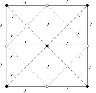
Figure 1: Ising model with nearest neighbor $J$ and diagonal $J^{\prime}$ interactions for the square lattice. Filled and open circles mean $s=+1$ and $s=-1$, respectively. Here, the usual two-sublattice arrangement of spins is shown.

Such a model correctly describes a planar array of $\pi$-rings deposited onto an insulating substrate. At each $\pi$-ring, there arises a magnetic orbital moment - an Ising spin. Such moments are oriented perpendicular to the plane and therefore they interact with each other via the long-range antiferromagnetic (dipole) interaction. Since such interactions decrease with a distance between moments as $~{}1/r^{3}$, i.e. very fast, we need to consider only interactions between the nearest and next-nearest neighboring spins, i.e. in the square lattice, there will be two constants of antiferromagnetic interaction, $J$ and $J^{\prime}$. Of course, due to the dipolar character of interaction the values of $J$ and $J^{\prime}$ for arrays of $\pi$-rings are related as $J^{\prime}=J/2^{3/2}$, but we consider a more general case, when their values are arbitrary.

For the planar systems of $\pi$-rings, the values of interactions $J$ and $J^{\prime}$ and their ratio can be externally controlled. One of the many possible way to control these interactions in the planar $\pi$-ring arrays is to introduce additional currents or current loops between the $\pi$-rings (see, Fig.2). In this figure, we consider a simplest square plaquette of $\pi$-rings. If the currents are flowing along the pairs of the straight lines in opposite directions, the magnetic field induced by these currents will influence the interaction between the $\pi$-rings and the ratio of the values $J/J^{\prime}$ will be changed. In a similar way, a controllable coupling of two loops, each consisting of the three-junction flux qubits, has been realized by inserting an additional current loop between them Ilichev . The $\pi$-ring is usually considered a primary candidate for the flux qubit due to a long decoherence time and low noises. The detailed measurements presented in Ref. Ilichev illustrate the flexibility of this two-loop tunable coupling that may be easily changed in a very broad range. The controllable adiabatic evolution of the multi $\pi$-ring systems, which we consider here, can be used for adiabatic quantum computation (AQC), see, for example, Ref. Ilichev1 , where the first experimental realization of AQC with the use of the controllable coupling has been realized. Bearing these experiments in mind, we consider small planar clusters of $\pi$-rings and analyze the diagrams of possible states for these small clusters at different values of the ratio $J/J^{\prime}$, which can arise via a controllable coupling.

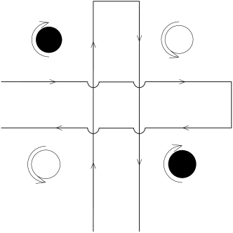
Figure 2: The smallest square cluster of $\pi$-rings, $2\times 2$. Here the value and the ratio of nearest-neighbor $J$ and diagonal $J^{\prime}$ interactions can be controlled by the external bias current $I$. The directions of currents in the $\pi$-rings and in control loops are indicated by arrows. Filled and open circles denote clockwise and counter-clockwise directed orbital currents associated with the orbital moments equal to $s=+1$ and $s=-1$, respectively.

III Thermal properties of small square plaquettes

III.1 A $2\times 2$ plaquette

The simplest cluster of $\pi$-rings, which may be easily built up experimentally is the square $2\times 2$ plaquette having four $\pi$-rings. The similar plaquette of $2\times 2$ superconducting loops has been build up and tested experimentally in the Ref. Ilichev3 . There was the first experimental demonstration of the working AQC device having the four qubits with a mixed couplings. The working circuit demonstrated in the Ref. Ilichev3 consisted of four three-junction loops – four flux qubits, with simultaneous ferro- and antiferromagnetic coupling implemented using shared Josephson junctions. The result obtained in the Ref. Ilichev3 gave a confidence that the similar working circuit based on four $\pi$-rings can be also implemented.

Such a $\pi$-ring cluster has $2^{4}=16$ distinct configurations that we label $0\ldots 15$. Converting these state labels to binary we have

Configuration	State	State	Configuration	State	State
0	0000	+ + + +	8	1000	- + + +
1	0001	+ + + -	9	1001	- + + -
2	0010	+ + - +	10	1010	- + - +
3	0011	+ + - -	11	1011	- + - -
4	0100	+ - + +	12	1100	- - + +
5	0101	+ - + -	13	1101	- - + -
6	0110	+ - - +	14	1110	- - - +
7	0111	+ - - -	15	1111	- - - -

Table 1: Possible configurations of a $2\times 2$ lattice illustrated by converting the binary form of the spin configuration into spin states

If there are only two types of coupling, $J$ and $J^{\prime}$, between all $\pi$-rings these states are associated with 4 different energies: 1) for the ferromagnetic state, $E_{++++}=4J+2J^{\prime}$; 2) for the one spin flop, $E_{+++-}=0$; 3) for the stripe order, $E_{++--}=-2J^{\prime}$ and 4) for the antiferromagnetic order, $E_{+-+-}=-4J+2J^{\prime}$. The corresponding spin configurations and the dependence of their energies on $J/J^{\prime}$ are shown in Figs. 3 and 4. At zero temperature, either the stripe order arising at $J/J^{\prime}<1$ or the antiferromagnetic or the checkerboard order, arising at $J/J^{\prime}>1$ will dominate. At zero or very low temperatures at slow changes of this ratio, the ground state adiabatically evolves from the checkerboard to the stripe order. The effective transition happens when $J=J^{\prime}$.

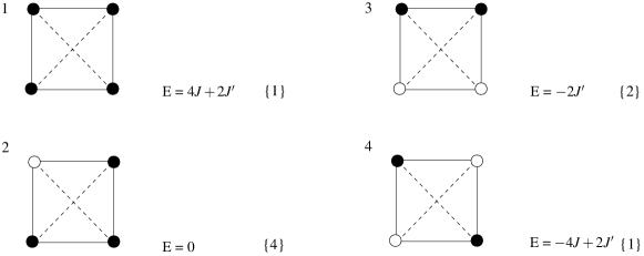
Figure 3: Possible nonequivalent spin configurations of a $2\times 2$ plaquette and the corresponding energies; the degree of degeneracy of each energy value is shown in curly brackets. The other 8 configurations are obtained by the reversal of all spins in the plaquette.

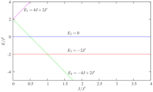
Figure 4: Energies of different states of a $2\times 2$ plaquette versus parameter $J/J^{\prime}$.

For a description of the evolution at any fixed temperature, we have to determine the partition function and the free energy of the system. We can populate our $2\times 2$ lattice with each of these enumerated states and sum up each contribution to get the partition function. Next, we find the free energy and the specific heat. Its maxima at the different ratio $J/J^{\prime}$ and the temperature $T$ give a phase diagram. This diagram indicates that such a toy adiabatic quantum computer operates well in the broad range of temperatures performing the adiabatic computation from the checkerboard to the stripe order, where the transition arising at the value $J=J^{\prime}$ is slightly smeared (see Fig. 5).

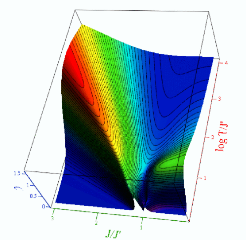
Figure 5: (color online) A three-dimensional plot of heat capacity $C$ versus $T/J^{\prime}$ and $J/J^{\prime}$ for a $2\times 2$ plaquette.

In a more general situation at the different coupling between different $\pi$-rings, any state enumerated in Table 1 may become a ground state that can be associated with some realistic problem needed to be solved with the AQC.

III.2 A 5-site plaquette: ground state and possible configurations

Of course, to go beyond such a toy computer we have to consider larger systems with large variety in the distribution of the coupling constants between the $\pi$-rings. We found that the behavior obtained for larger clusters is very different from one obtained above. The next system which, nonetheless, may already have nontrivial generic features is a cluster (plaquette) consisting of five $\pi$-rings. Its central cite has four neighbors. For the further analysis, we choose this plaquette of minimum size, because it retains the symmetry and the characteristic geometry of the lattice as a whole (the number of nearest-neighbor and diagonal bonds are equal, see Fig. 6). The properties of such plaquette consisting of 5 $\pi$-rings may be generic to develop a scalable architecture for AQC.

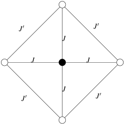
Figure 6: Square plaquette of the minimum size (with the equal number of of nearest-neighbor and diagonal bonds).

The possible configurations of this 5-site plaquette are easily listed (we have $2^{5}=32$ configurations with different values of energy), see Fig. 7. In Fig. 8, we plot the dependence of energies for the lowest energy states (states 1, 2, 3, and 4) on the $J/J^{\prime}$ ratio.

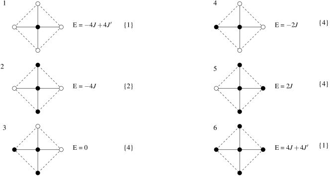
Figure 7: Possible spin configurations of a 5-site plaquette and the corresponding energies; the degree of degeneracy of each energy value is shown in curly brackets. Only 16 configurations with the filled circle in the center are shown; there are also 16 similar configurations with the open circle in the center of the plaquette.

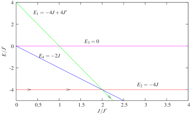
Figure 8: Energies of different states of a 5-site plaquette versus parameter $J/J^{\prime}$. The solid line with arrows illustrates the variation of parameters corresponding to the adiabatic computations.

One can see that state 1 corresponding to the usual two-sublattice antiferromagnetism (the checkerboard arrangement of filled and open circles) is favorable at $J/J^{\prime}>2$, whereas state 2 corresponding to the alternation of chains formed by filled and open circles becomes favorable at rather large magnitude of the diagonal interaction, $J/J^{\prime}<2$. Note that for state 4, plot $E_{4}(J/J^{\prime})$ also passes through the crossing point of $E_{1}(J/J^{\prime})$ and $E_{2}(J/J^{\prime})$. State 4 could be treated as a defect in regular lattices corresponding to states 1 and 2. So, the crossing of plots at $J/J^{\prime}=2$ gives a clear indication of a possible formation of some more complicated phases near this point. Indeed, an almost zero barrier to the formation of defects, like domain boundaries and dislocations, is usually a good signature of the situation when some kind of superstructure could be favorable. For the case of AQC, the computation process may start from the $\pi$-ring cluster, where the value of $J/J^{\prime}>2\sqrt{2}$. There, the ground state must correspond to the plain checkerboard antiferromagnetic order. If we slowly decrease the $J/J^{\prime}$ ratio the system will inevitably evolve to the stripe structure. This demonstrates the proper operation of the AQC having 5 qubits. However, at nonzero temperatures the situation is much more subtle than that.

III.3 A 5-site plaquette: partition function, free energy, and peaks in specific heat

Now, let us discuss the behavior of the 5-site plaquette at finite temperatures. Knowing the set of energy levels and their degeneracy (see Fig. 7), we can easily write the partition function in the form (the Boltzmann constant is taken to be equal to one)

$$Z=2\left[e^{\frac{4J-4J^{\prime}}{T}}+2e^{\frac{4J^{\prime}}{T}}+4+4e^{\frac{2J}{T}}+4e^{\frac{-2J}{T}}+e^{\frac{-4J-4J^{\prime}}{T}}\right]=$$

$$=8\left[e^{\frac{-4J^{\prime}}{T}}\cosh\frac{2J}{T}+2\cosh\frac{2J}{T}+2\sinh\frac{4J^{\prime}}{T}+1\right].$$ (2)

Free energy $F$ and heat capacity $C$ for the plaquette are given by standard thermodynamic formulas $F=-T\ln Z$ and $C=-T\frac{\partial^{2}F}{\partial T^{2}}$. Then, the peaks in the $C(T)$ curves at different values of $J/J^{\prime}$ can be treated as manifestations of phase transitions, which are going to occur for the infinite lattice. From this viewpoint, let us analyze the low-temperature behavior of the heat capacity.

From the usual expression for the heat capacity

$$C(T)=-T\frac{\partial^{2}F}{\partial T^{2}}=\frac{2T}{Z}\frac{\partial Z}{\partial T}-\frac{T^{2}}{Z^{2}}\left(\frac{\partial Z}{\partial T}\right)^{2}+\frac{T^{2}}{Z}\frac{\partial^{2}Z}{\partial T^{2}},$$ (3)

we can see that the structure of the $C(T)$ function is such that it is possible to get rid of the growing exponentials in the partition function, $Z$, by dividing both numerator and denominator in $C(T)$ by the largest exponential. Then, we can work with exponentials having negative arguments. Indeed, let

$$Z=A^{\prime}e^{\frac{A}{T}}(1+Be^{-\frac{D}{T}}+\ldots).$$ (4)

From Eq. (3), it obvious that $C(T)$ does not depend either on $A$ or on $A^{\prime}$. In the low-temperature limit, taking into account only the terms proportional to $e^{-\frac{D}{T}}$, we find

$$C(T)\approx\frac{BD^{2}}{T^{2}}e^{-\frac{D}{T}}.$$ (5)

Note that the terms $\sim e^{-\frac{D}{T}}/T$ are cancelled. Using expression (5) and condition $dC/dT=0$, we find temperature $T_{c}$ corresponding to the position of the heat capacity peak (in the limit $T\rightarrow 0$)

$$T_{c}=\frac{D}{2}.$$ (6)

Let us introduce for convenience the following dimensionless variables

$$f=\frac{F}{J^{\prime}},\quad t=\frac{T}{J^{\prime}},\quad\alpha=\frac{J}{J^{\prime}}.$$ (7)

In this notation, Eq. (III.3) for the partition function can be rewritten in the following way

$$Z=2\left[e^{\frac{4\alpha-4}{t}}+2e^{\frac{4}{t}}+4+4e^{\frac{2\alpha}{t}}+4e^{\frac{-2\alpha}{t}}+e^{\frac{-4-4\alpha}{t}}\right].$$ (8)

As it was mentioned above, to analyze the low-temperature limit, it is reasonable to retain only growing exponentials in Eqs. (III.3) or (8). Thus, we get

$$Z\approx 2\left[e^{\frac{4\alpha-4}{t}}+2e^{\frac{4}{t}}+4e^{\frac{2\alpha}{t}}\right].$$ (9)

At $\alpha=\frac{J}{J^{\prime}}>2$, we can write the partition function in the form similar to (4)

$$Z\approx 2e^{\frac{4J-4J^{\prime}}{T}}(1+4e^{-\frac{D_{1}}{T}}+\ldots),$$ (10)

where $D_{1}=2J-4J^{\prime}$.

In the case $\alpha=\frac{J}{J^{\prime}}<2$, we find

$$Z\approx 4e^{\frac{4J^{\prime}}{T}}(1+4e^{-\frac{D_{2}}{T}}+\ldots),$$ (11)

where $D_{2}=4J^{\prime}-2J$.

As a result, using (6), we find the following positions of the heat capacity peaks in the low-temperature limit

$$\alpha=2+t,\quad\alpha>2.$$ (12)

$$\alpha=2-t,\quad\alpha<2.$$ (13)

Plotting the positions of heat capacity maxima in the $t-\alpha$ plane yields a kind of phase diagram for a small plaquette. Indeed, the positions of $C(t,\alpha)$ peaks could be related to the actual phase transitions occurring in infinite systems. Such a phase diagram for the plaquette under study is shown in Fig. 9. Note that at $\alpha<2$, the lowest energy corresponds to plaquette 2 in Fig. 7 (chains of spins with the same direction), whereas at $\alpha>2$, plaquette 1 (two-sublattice checkerboard antiferromagnetism) is the most favorable. However, at non-zero temperatures, there is no boundary between these two phases. Instead, we have a whole quadrant in the $t-\alpha$ plane (with the vertex at point (0, 2)), where one could expect for the infinite lattice numerous phases, intermediate between the two-sublattice and chain-like structures. The situation is very much alike that of the ANNNI model SelkePRep , where the “devil’s staircase” of different phases arises at finite temperatures between two main phases existing at zero temperature. Region 3 within this quadrant is bounded by a curve corresponding to the positions of an additional (high-temperature) peak in the temperature dependence of the heat capacity. So, this is another indication that for larger clusters, and in the infinite system, one should expect in this range a phase with a certain kind of ordering, maybe quite unusual, rather than simply a disordered paramagnetic phase. For illustration, we present here also a three-dimensional plot of heat capacity $C(t,\alpha)$ (see Fig. 10) corresponding to the phase diagram shown in Fig. 9.

Figure 9: “Phase diagram”(positions of the heat capacity peaks) for a 5-site plaquette in the $t-\alpha$ plane. Region 1 corresponds to state 1 of the plaquette (see Fig. 7), region 2 could be related to state 2 of the plaquette. In region 3, one could expect for the corresponding infinite square lattice multiple phases (similar to those in the ANNNI model) or a phase with a complicated spin ordering.

To summarize, when the ratio $J/J^{\prime}$ is in the vicinity of the value 2 for the plaquette cluster of five $\pi$-rings, the antiferromagnetic, checkerboard ground state (1) having zero entropy (nondegenerate) is very difficult to reach. So, the system is practically always disordered due to a proliferation of defects (4), see, Figs. 3 and 8. This diagram also indicates that some problems arise even for the toy 5-$\pi$-ring adiabatic quantum computer. Although it operates well at zero temperature, in very broad range of low temperatures performing adiabatic computations such as the adiabatic evolution from the checkerboard to the stripe order may have an obstacle in the form of the proliferation of topological defects inherently presented in the phase (3). Now, we would like to show that these difficulties with AQC even are enhanced in the case of larger clusters. Also, the broad peak in specific heat indicates that a true phase transition may arise for a large system of $\pi$-rings.

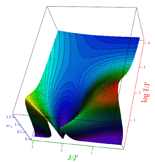
Figure 10: A three-dimensional plot of heat capacity $C$ versus $t=T/J^{\prime}$ and $\alpha=J/J^{\prime}$, which corresponds to the phase diagram shown in Fig. 9.

IV Exact solutions for larger plaquettes

In the previous Section, we found all possible energy states for the 5-site plaquette, see Fig. 7. For a small portion of the square lattice (less than about $4\times 4$ sites), it is possible to list its different spin configurations and calculate the macroscopic quantities exactly. For a $3\times 3$ site lattice we find that there are 11 different energies associated with $2^{9}$ different states and can rather easily reproduce the analysis of the minimum of energy but due to its small size this is of limited value. For a $5\times 5$-site square, there are already 161 different energy levels and thus the approach used in the previous Section seems to be impractical.

A $5\times 5$-site lattice has $2^{25}\approx 3\times 10^{7}$ distinct configurations that can be enumerated by converting each state ($0\ldots 2^{N}-1$) into a binary number where the 0 or 1 digit of the binary form corresponds to an up or down spin in our Hamiltonian (similarly to the notation introduced in Table 1 for the $2\times 2$ plaquette). With the use of such enumeration, we calculate the partition function function of the lattice and thus deduce the macroscopic quantities of interest by numerically differentiating the partition function using the usual finite difference schemes. As a result, for larger square plaquettes (say, with $4\times 4$ and $5\times 5$ sites), we can find their heat capacity and draw 3D plots similar to that shown in Fig. 10, which illustrate the phase diagram of these plaquettes. The corresponding plots for $4\times 4$- and $5\times 5$-site squares are shown in Figs. 11 and 12. The qualitative features of these plots reproduce the situation characteristic of the 5-site plaquette discussed in the previous Section. Note, however, that cutting from the infinite square lattice finite $N\times N$-site pieces (with the cuts parallel to $x$ and $y$ axes), we get square plaquettes with unequal number of $J$ and $J^{\prime}$ bonds. The corresponding “surface contribution” can affect the specific form of the phase diagram, especially, in the regime of the strong degeneracy, when $J/J^{\prime}=2$.

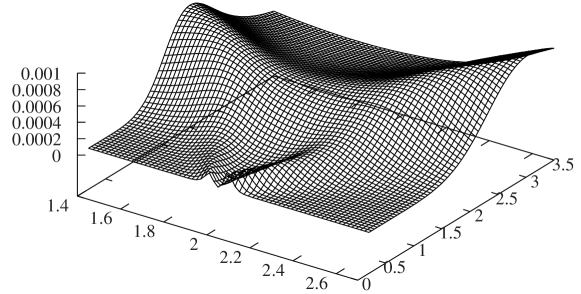
Figure 11: A three-dimensional plot of heat capacity $C$ versus $t=T/J^{\prime}$ and $\alpha=J/J^{\prime}$ for a $4\times 4$ square plaquette.

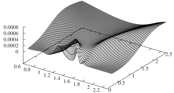
Figure 12: A three-dimensional plot of heat capacity $C$ versus $t=T/J^{\prime}$ and $\alpha=J/J^{\prime}$ for a $5\times 5$ square plaquette.

V Square infinite lattice: semiqualitative analysis and energetics of topological defects

Let us discuss the possible spin configurations corresponding to Hamiltonian (1) for the infinite square lattice. Two configurations, which may have the lowest energy per site at large and small ratio of coupling constants $J/J^{\prime}$ are shown in Fig. 13.

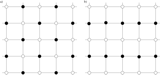
Figure 13: Two types of spin ordering corresponding to the lowest energy for the square lattice with the the antiferromagnetic nearest-neighbor $J$ and diagonal $J^{\prime}$ interactions: (a) two-sublattice classical antiferromagnetism (diagonal stripes) arising when $J/J^{\prime}\gg 1$ and (b) chain-like antiferromagnetic ordering (horizontal stripes) arising when $J/J^{\prime}<<1$. The rotation of configuration (b) by 90^∘ gives vertical stripes with the same energy.

For diagonal stripes, we gain energy at nearest-neighbor interactions and loose energy at diagonal bonds, hence this configuration is the most favorable at $J/J^{\prime}\gg 1$. For the horizontal (vertical) stripes, the main energy gain comes from the diagonal neighbors, and it becomes favorable at large values of $J^{\prime}$ ($J/J^{\prime}\ll 1$). The corresponding energies (per site) are

$$E_{ds}=-2J+2J^{\prime}\quad\text{for diagonal stripes},$$ (14)

$$E_{hs}=-2J^{\prime}\quad\text{for horizontal (vertical) stripes}.$$ (15)

The transition between diagonal and horizontal stripe states ($E_{ds}=E_{hs}$) occurs at

$$J/J^{\prime}=2.$$ (16)

Let us now discuss the possible types of defects and phase boundaries, which could arise in our model.

First, let us analyze the state with horizontal or vertical stripes. The most natural defect for this state is just the boundary between the domains corresponding to vertical and horizontal stripes (see Fig. 14).

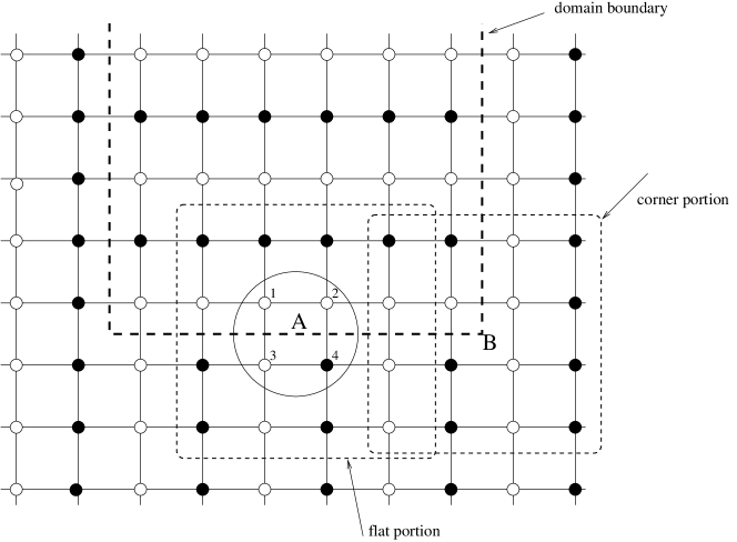
Figure 14: Domain boundary between horizontal and vertical stripes (horizontal or vertical boundary).

Let us now calculate the energy (per site) for the flat portion of this domain boundary. We take a 4-site plaquette around point A in Fig. 14 and calculate energies of sites numbered from 1 to 4. Thus, we have

$$E_{1}=\frac{1}{2}\left[-4J^{\prime}+3J-J\right]=-2J^{\prime}+J,$$

$$E_{2}=\frac{1}{2}\left[-2J^{\prime}+2J^{\prime}-2J+2J\right]=0,$$

$$E_{3}=\frac{1}{2}\left[-2J^{\prime}+2J^{\prime}+2J-2J\right]=0,$$

$$E_{4}=\frac{1}{2}\left[-4J^{\prime}+J-3J\right]=-2J^{\prime}-J,$$

$$E_{fp}=\frac{1}{4}\left[E_{1}+E_{2}+E_{3}+E_{4}\right]=-J^{\prime}.$$ (17)

The same calculation can be performed for the corner portion of this domain boundary (see four sites surrounding point B in Fig. 8). After the procedure similar to that presented by Eq. (V), we find

$$E_{cp}=-J^{\prime}.$$ (18)

So, we see that $E_{cp}=E_{fp}$, that is, kinks at the domain boundary do not cost additional energy. This means that at finite temperatures, the formation of polygonal domain boundaries could be favorable from the viewpoint of the configurational entropy.

In addition to the domain boundaries along the vertical and horizontal axes, it is possible to consider also a diagonal domain boundary illustrated in Fig. 15.

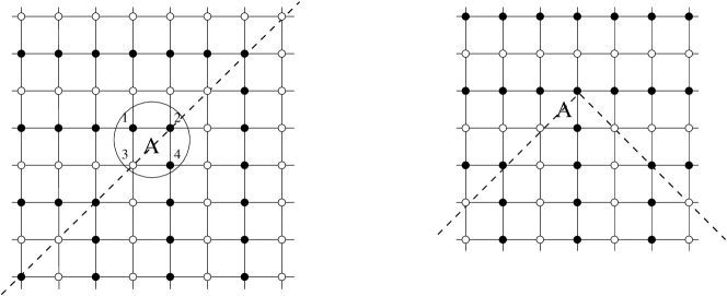
Figure 15: Diagonal domain boundary for the phase with horizontal and vertical stripes (left panel) and the corner portion for this type of domain boundary (right panel).

Again, calculating the energies of four sites surrounding point A in the left panel of Fig. 15, we find

$$E_{1}=\frac{1}{2}\left[-2J+2J-3J^{\prime}+J^{\prime}\right]=-J^{\prime},$$

$$E_{2}=\frac{1}{2}\left[-2J+2J-4J^{\prime}\right]=-2J^{\prime},$$

$$E_{3}=\frac{1}{2}\left[-2J+2J-4J^{\prime}\right]=-2J^{\prime},$$

$$E_{4}=\frac{1}{2}\left[-2J+2J-3J^{\prime}+J^{\prime}\right]=-J^{\prime},$$

$$E_{fp}=\frac{1}{4}\left[E_{1}+E_{2}+E_{3}+E_{4}\right]=-\frac{3}{2}J^{\prime}.$$ (19)

So, we see that the diagonal domain boundary has even lower energy than the vertical and horizontal boundaries. The corner portion of this kind of domain boundary is illustrated in the right panel of Fig. 15. The energy per site for this corner portion can be found by considering the neighbors of site A in the right panel of Fig. 15. Thus, we have

$$E_{cp-d}=-2J^{\prime}+J.$$ (20)

At large $J^{\prime}$, this energy can be even smaller than that given by Eq. V.

In addition to the domain boundaries, there are also dislocations of the type shown in Fig. 16.

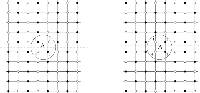
Figure 16: A dislocation(shift by one lattice constant) in the phases with horizontal and vertical stripes (left panel) and with diagonal stripes (right panel).

Calculating the energy of four spins around point A in the left panel of Fig. 16, we find that the energy of such a dislocation per site is

$$E_{disl}=-J.$$ (21)

The corresponding type of dislocations also exists for the phase with diagonal stripes, see right panel of Fig. 16. Again, calculating the energy of four spins around point A in the right panel of Fig. 16, we find that the energy of the dislocation equal to that for the dislocation shown in the left panel of Fig. 16

$$E^{\prime}_{disl}=-J.$$ (22)

Now, let us consider the energy of phase boundaries between phases with horizontal/vertical and diagonal stripes. Two types of such a boundary are illustrated in Fig. 17.

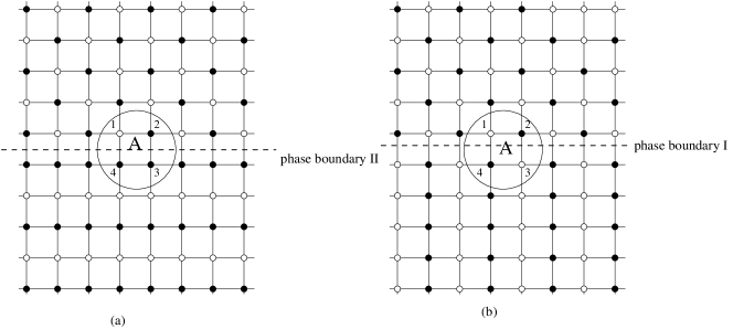
Figure 17: Boundaries between phases with with diagonal stripes and (a) horizontal and (b) vertical stripes.

Following the same procedure of calculating the energies of four sites around point A both in panels (a) and (b) in Fig. 17, we find the values of energy per site corresponding to phase boundaries I and II. Thus, we have

$$E_{pbI} = -\frac{3}{2}J+J^{\prime},$$

$$E_{pbII} = 0.$$ (23)

The energies of all phases and defects per site are summarized in Fig. 18.

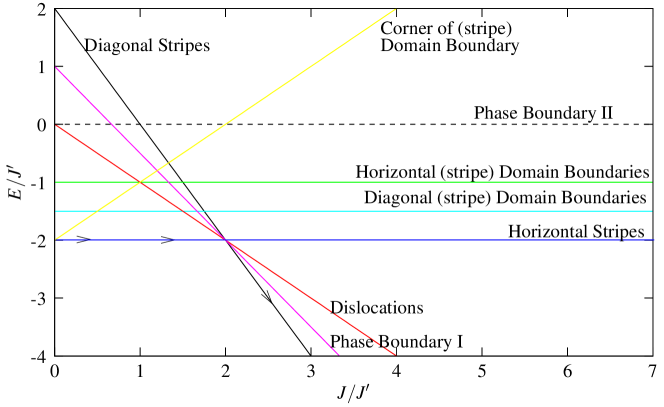
Figure 18: (Color online) Energies (per site) of different phases and main topological defects for the square Ising lattice with nearest-neighbor and diagonal interactions versus parameter $\alpha=J/J^{\prime}$. The solid line with arrows illustrates the variation of parameters corresponding to the adiabatic computations, similarly to that in Fig. 8.

From Fig. 18, we can see that the crossing point of energies for phases with diagonal and horizontal/vertical stripes ($J/J^{\prime}=2)$ is also the crossing point for the energies of dislocations. On the other hand, the entropy of a state with the defects is significantly larger than the entropy of a plain disordered state. This implies, of course, the possibility of the creation of dislocations near the crossover between these two phases. Therefore, at nonzero low temperatures, the defects described above will proliferate into the ordered antiferromagnetic checkerboard and stripy states. The proliferation phenomenon occurs within a broad range of $J/J^{\prime}$ values. Due to this proliferation of topological defects, there arises a problem with performing AQC. It has the same origin as we have discussed for the five-$\pi$-ring plaquette. Namely, during adiabatic evolution of the ground state, i.e. the antiferromagnetic checkerboard state, when the ratio $J/J^{\prime}$ decreases, the system will enter into the intermediate phase characterized by a creation of a large number different topological defects. Such topological defects are quite stable and may have a very long lifetime provided that they do not annihilate with each other like vortices with antivortices. As the result of this adiabatic evolution a some number of defects will definitely proliferate into the final ground state and therewith may introduce an error in the adiabatic quantum computation. At present, we do not know, how to resolve this issue of the spontaneous creation of topological defects during the AQCs with the larger clusters. Note that even for the case of the planar array of the $\pi$-rings, when the coupling is not tuned and the value $\alpha=2\sqrt{2}$, we expect that the proliferation of the defects will strongly modify the ordered antiferromagnetic state. The similar possibility was also revealed in the analysis of thermodynamics of a 5-site plaquette.

VI Adiabatic quantum computations with a planar array of $\pi$-rings and conclusion

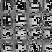
(a) $t=T/J^{\prime}=0.1$

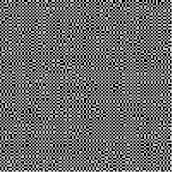
(b) $t=T/J^{\prime}=0.25$

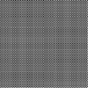
(c) $t=T/J^{\prime}=1.0$

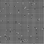
(d) $t=T/J^{\prime}=2.5$

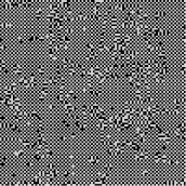
(e) $t=T/J^{\prime}=3.0$

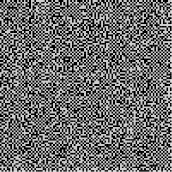
(f) $t=T/J^{\prime}=4.0$

Figure 19: The result of Monte Carlo simulations of the spin structure for the $100\times 100$ square Ising lattice with competing antiferromagnetic interactions at $\alpha=J/J^{\prime}=2\sqrt{2}$. Dark and light square cells correspond to $s=+1$ and $s=-1$, respectively.

Now, it is interesting to consider a realistic system, where the physical phenomenon of the proliferation of defects described above can be realized. The first choice is the planar array made of $\pi$-rings. We would like to consider a large system like a $100\times 100$ square lattice with Ising spins having competing antiferromagnetic interactions at arbitrary value of $\alpha=J/J^{\prime}$. The specific case of the dipole-dipole interaction between isolated $\pi$-rings deposited onto a dielectric substrate will correspond to the value $\alpha=2\sqrt{2}$. We performed the numerical simulation of this system using the Monte Carlo method, which is the only method available to treat such large systems. Let us demonstrate the results of the Monte Carlo simulation at various temperatures ($T/J^{\prime}=0.01-5.0$). The spin structure for the $100\times 100$ square Ising lattice with competing antiferromagnetic interactions at $\alpha=J/J^{\prime}=2\sqrt{2}$ is presented in Fig. 19, where each square in this figure corresponds to the $\pi$-ring. The dark square corresponds to the up-spin orientation of the orbital moment, while the light square corresponds to the down-spin orientation of the orbital moment. At this value of $\alpha=2\sqrt{2}$ corresponding to the square array of $\pi$-rings (see, the Ref. KirtleyPRB05 ), at low temperatures we should expect a usual two-sublattice antiferromagnetic ordering of Ising spins. Instead, we see a complicated array, a mixture of light and dark squares. The two-sublattice portions are mixed with the topological defects like dislocations and domain boundaries. This picture is in the agreement with our previous discussion demonstrating the possibility of a rather low energy barrier and large entropy for the creation of defects. A similar picture of the spin distribution was also observed in experiments with the arrays of $\pi$-rings KirtleyPRB05 .

Let us discuss the possibility to use a large planar arrays of $\pi$-rings for adiabatic quantum computations. The semiqualitative discussion presented in this paper clearly demonstrates that the clusters of $\pi$-rings may be perfectly described by the Ising model with competing nearest-neighbor and diagonal interactions. The system exhibits a plethora of unusual properties, which are promising for the analysis of various analogous physical systems of different nature and also for studies of different AQC algorithms. However, as we discussed above, the proliferation of topological defects arising in the process of AQC may contribute an error into the final result. The physical phenomenon of the proliferation of defects described for the planar array made of $\pi$-rings may also lead to a formation of a new type of glassy state OHare .

Recently, a scalable design for adiabatic quantum computations has been proposed and realized Zakosarenko . The key element of this design is a coupler, which is a ring with a single Josephson junction that provides a controllable coupling between two bistable flux qubits. The similar tunable coupling may be realized for the large $\pi$-ring arrays, which we discuss here. Now let us investigate how good is to use such $\pi$-ring arrays with controllable coupling for adiabatic quantum computations. Such arrays are well described by the Ising model with competing interactions as we discussed in the paper. The adiabatic quantum computer based on such large $\pi$-ring arrays with the controllable coupling will be able to solve a very limited range of problems. In many cases they are still toy problems, which serve as a polygon towards future developments for various realistic applications. One of such applications is a Travelling Salesman Problem Kieu , which can be represented in the form of more complicated Ising model, with a set of a coupling constants Tosatti1 .

Now let us investigate the process of the adiabatic evolution of $100\times 100$ $\pi$-ring array when the coupling between all $\pi$-rings is tuned simultaneously in a way that the ratio $\alpha=J/J^{\prime}$, which is the ratio of exchange constants in the corresponding Ising model, increases from zero. First, we consider zero or very close to zero temperatures. When the value of $\alpha$ is small we have a well defined ground state – the stripe phase. The distribution of spins for such a state form stripes oriented horizontally or vertically. So, it is double degenerate and, therefore, there is a possibility to form two types of domains associated with horizontal and vertical stripe phases as discussed in the previous sections. When the parameter $\alpha$ increases adiabatically according to the adiabatic theorem (see, a detail discussion of the application of this theorem to quantum adiabatic computations given in Ref. Kieu1 ) the system will remain in the ground state. For small temperature the domain walls and domains may still proliferate into the system but if they do, their number is very small. When the parameter $\alpha$ approaches to the value $\alpha=1$, the proliferation of numerous domain walls and other types of topological defects such as dislocations and phase boundaries described in the previous section should arise. Within the $1<\alpha<2$ range, the state is highly disordered. The formation of such disordered structures in the $\pi$-ring arrays arising during the adiabatic evolution in the course of tuning the coupling constants may be explained by the presence of strong frustrations in this system. The frustration reaches its maximum in the vicinity of the value $\alpha=2$.

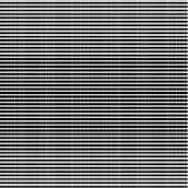
(a) $\alpha=J/J^{\prime}=1.0$

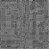
(b) $\alpha=J/J^{\prime}=1.6$

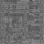
(c) $\alpha=J/J^{\prime}=1.8$

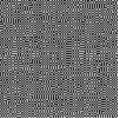
(d) $\alpha=J/J^{\prime}=2.0$

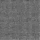
(e) $\alpha=J/J^{\prime}=2.4$

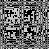
(f) $\alpha=J/J^{\prime}=3.4$

Figure 20: The result of Monte Carlo simulations of the spin structure for the $100\times 100$ square Ising lattice with competing antiferromagnetic interactions at different $\alpha=J/J^{\prime}$ and at fixed low temperature $T/J^{\prime}=0.1$. Dark and light square cells correspond to $s=+1$ and $s=-1$, respectively.

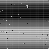
(a) $\alpha=J/J^{\prime}=1.0$

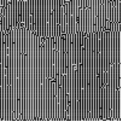
(b) $\alpha=J/J^{\prime}=1.6$

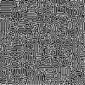
(c) $\alpha=J/J^{\prime}=1.8$

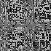
(d) $\alpha=J/J^{\prime}=2.0$

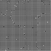
(e) $\alpha=J/J^{\prime}=2.4$

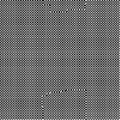
(f) $\alpha=J/J^{\prime}=3.4$

Figure 21: The result of Monte Carlo simulations of the spin structure for the $100\times 100$ square Ising lattice with competing antiferromagnetic interactions at different $\alpha=J/J^{\prime}$ and at fixed temperature $T/J^{\prime}=1.5$. Dark and light square cells correspond to $s=+1$ and $s=-1$, respectively.

Figure 22: A schematic phase diagram the 2D Ising model with competing interactions on a square lattice based on the Monte Carlo calculations of heat capacity for the $100\times 100$ square plaquette. The lower branch corresponds to the boundary of the glassy state and the upper branch is the boundary of the phases with the long-range spin order.

Our estimation indicate that in this $\alpha$ parameter range the energies of many topological defects, like domain walls between different antiferromagnetic phases as well as various dislocations, are very close to the ground state energy. Therefore, there appear many locally stable (or metastable) states associated with local energy minima separated by energy barriers (see, Fig. 20d). With the further increase of $\alpha$, the energy barriers separating these metastable states increase. During the adiabatic evolution the system may be trapped into one of these metastable minima. After that, during the subsequent adiabatic evolution, it will have not enough time to leave this metastable minimum and and therefore the system will remain in the disordered state associated with this minimum. In fact, during this mass proliferation of topological defects, we enter into the disordered glassy state OHare ; Tosatti . The glassy state consists of many equivalent minima. Obviously during the adiabatic computing the system will be trapped in one of them. If we repeat the adiabatic computing once more, the system may be trapped into another equivalent minimum of the glassy state. Performing this AQC many time a complicated glassy state in a form of a large number of disordered ground states associated with closed energies may be reproduced. For $\pi$-ring clusters, there is a straightforward way to read out the final result in the form of the configuration of the orbital moments, as it was done in the Ref. KirtleyNature . The adiabatic computing processes described here may lead to the same results as in the case of the thermal relaxation but can be sometimes significantly faster, see e.g. Ref. Zagoskin .

Thus, we see that the adiabatic evolution of the system may lead to an efficient adiabatic computation corresponding to a very complicated ground state, which can be characterized by the Edwards-Anderson order parameter EdwAnd . The final result of this evolution is quite nontrivial: a glassy state associated with frustrations. It is also very interesting to investigate, how such adiabatic evolution will depend on temperature, especially taking into account that the thermal environment can enhance the performance of adiabatic computations TherAssAQC . Note here that an increase in temperature could help one to avoid trapping the system into a complicated glassy state. This situation is illustrated in Fig. 21. It corresponds to the same variation of the $J/J^{\prime}$ parameter as in Fig. 20, but at higher temperature $T/J^{\prime}=1.5$. We see that in contrast to the low-temperature case, it is possible to pass from the stripe phase to the checkerboard antiferromagnetic phase without being trapped in the glassy state. Here, only in the vicinity of $J/J^{\prime}=2$, the system exhibits a pronounced disorder. In general, let us note that the use of the evolution of the physical system for the computing is quite powerful idea. It can be used at low temperatures, where computations may have some quantum characters relying on a long decoherence time. However, an adiabatic evolution of large physical systems may be used for computations in a much broader sense and at high temperatures, as it was demonstrated in Fig. 21. We hope that these ideas will be exploited further. The possible kinds of behavior are summarized in the schematic phase diagram (Fig. 22) based on the Monte Carlo calculations of the heat capacity for the $100\times 100$ square plaquettes. This figure demonstrates that the glassy state arising at the value $J/J^{\prime}>1$ is favorable at low temperatures, whereas in the intermediate temperature range, there exists a crossover between different types of the long-range spin order.

A detailed description of other results for the Ising model with competing interactions that include the Monte Carlo simulations for the spin structure, phase diagram, and spin correlation functions, as well as analytical and numerical results obtained by the transfer matrix technique, will be presented in a separate publication.

References

- (1) R. J. Elliott, Phys. Rev. 124, 346 (1961).
- (2) M. E. Fisher and W. Selke, Phys. Rev. Lett. 44, 1501 (1980).
- (3) P. Bak, Phys. Today 39, 38 (1986).
- (4) P. Bak and R. B. Bruinsma, Phys. Rev. Lett. 49, 249 (1982).
- (5) P. Bak and P. von Boehm, Phys. Rev. B21, 5297 (1980).
- (6) W. Selke, Phys. Reports 170, 212 (1988).
- (7) T. Kimura, S. Ishihara, H. Shintani, T. Arima, K. T. Takahashi, R. Ishizaka, and Y. Tokura, Phys. Rev. B68, 060403(R) (2003).
- (8) R. Moessner, Can. J. Phys. 79, 1283 (2001); R. Moessner and S. L. Sondhi, Phys. Rev. B63, 224401 (2001).
- (9) C. Fan and F.Y. Wu, Phys. Rev. 179, 560 (1969).
- (10) D.P. Landau and K. Binder, Phys. Rev. B31, 5946 (1985).
- (11) T.D. Grynberg and B. Tatanar, Phys. Rev. B45, 2876 (1992).
- (12) A. Malakis, P. Kalozoumis, and N. Tyraskis, Eur. Phys. J. B 50, 63 (2006).
- (13) F.V. Kusmartsev, Phys. Rev. Lett. 69, 2268 (1992).
- (14) E. Farhi, J. Goldstone, S. Gutmann, and M. Sipser, Quantum computation by adiabatic evolution, quant-ph/0001106.
- (15) H. Hilgenkamp, Ariando, H.-J. H. Smilde, D. H. A. Blank, G. Rijnders, H. Rogalla, J. R. Kirtley, and C. C. Tsuei, Nature (London) 422, 50 (2003).
- (16) J. R. Kirtley, C. C. Tsuei, Ariando, H. J. H. Smilde, and H. Hilgenkamp, Phys. Rev. B72, 214521 (2005).
- (17) P. Svedlindh, K. Niskanen, P. Norling, P. Nordblad, L. Lundgren, B. Lönnberg, and T. Lundström, Physica C 162-164, 1365 (1989).
- (18) W. Braunisch, N. Knauf, V. Kataev, S. Neuhausen, A. Grütz, A. Kock, B. Roden, D. Khomskii, and D. Wohlleben, Phys. Rev. Lett. 68, 1908 (1992).
- (19) M.L. Della Rocca, M. Aprili, T. Kontos, A. Gomez, and P. Spathis, Phys. Rev. Lett. 94, 197003 (2005).
- (20) M. Aprili, T. Kontos, W. Guichard, J. Lesueur, and P. Gandit, Physica C 408-410, 606 (2004).
- (21) F. V. Kusmartsev, D. M. Forrester, and M. S. Garelli, Fractal structures in a chain of SQUIDs with -shifts, in book of abtracts Physics of Superconducting Phase Shift Devices, ed. A. Barone et al., Ischia (Napoli), April 2–5, p. 21 (2005).
- (22) D.M. Forrester, K.E. Kürten, and F.V. Kusmartsev, Phys. Rev. B75, 014416 (2007).
- (23) K.E. Kürten and F.V. Kusmartsev, Phys. Rev. B72, 014433 (2005).
- (24) M. Grajcar, A. Izmalkov, and E. Il’ichev, Phys. Rev. B71, 144501 (2005).
- (25) R.P. Feynman, Int. J. Theor. Phys. 21, 467 (1982)
- (26) S.H.W. van der Ploeg, A. Izmalkov, Alec Maassen van den Brink, U. Hübner, M. Grajcar, E. Il’ichev, H.-G. Meyer, and A.M. Zagoskin, Phys. Rev. Lett. 98, 057004 (2007).
- (27) S.H.W. van der Ploeg, A. Izmalkov, M. Grajcar, U. Hübner, S. Linzen, S. Uchaikin, Th. Wagner, A. Yu. Smirnov, A. Maassen van den Brink, M. H.S. Amin, A.M. Zagoskin, E. Il’ichev and H.-G. Meyer, Adiabatic quantum computation with flux qubits, first experimental results. cond-mat/0702580.
- (28) M. Grajcar, A. Izmalkov, S.H.W. van der Ploeg, S. Linzen, T. Plecenik, Th.Wagner, U. Hübner, E. Il’ichev, H.-G. Meyer, A.Yu. Smirnov, Peter J. Love, Alec Maassen van den Brink, M.H.S. Amin, S. Uchaikin, and A.M. Zagoskin, Phys. Rev. Lett. 96, 047006 (2006).
- (29) A. O’Hare, F.V. Kusmartsev, M.S. Laad, and K.I. Kugel, Physica C 437-438, 230 (2006).
- (30) V. Zakosarenko, N. Bondarenko, S.H.W. van der Ploeg, A. Izmalkov, S. Linzen, J. Kunert, M. Grajcar, E. Il’ichev, and H.-G. Meyer, Appl. Phys. Lett. 90, 022501 (2007).
- (31) Tien D. Kieu, Quantum adiabatic computation and traveling salesman problem, quant-ph/0601151.
- (32) Roman Martoňàk, Giuseppe E. Santoro, and Erio Tosatti, Phys. Rev. E 70, 057701 (2004)
- (33) Tien D. Kieu, Contemp. Phys. 44, 51 (2003).
- (34) Giuseppe E. Santoro, Roman Martoňàk, Erio Tosatti, and Roberto Car, Science 295, 2427 (2002).
- (35) A.M. Zagoskin, S. Savel ev, and Franco Nori, Phys. Rev. Lett. 98, 120503 (2007).
- (36) S. F. Edwards and P. W. Anderson, J. Phys. F 5, 965 (1975).
- (37) M.H.S. Amin, Peter J. Love, and C.J.S. Truncik, cond-mat/0609332.