A Coarse graining for the Fortuin-Kasteleyn measure in random media

Abstract

By means of a multi-scale analysis we describe the typical geometrical structure of the clusters under the FK measure in random media. Our result holds in any dimension $d\geqslant 2$ provided that slab percolation occurs under the averaged measure, which should be the case in the whole supercritical phase. This work extends the one of Pisztora [29] and provides an essential tool for the analysis of the supercritical regime in disordered FK models and in the corresponding disordered Ising and Potts models.

1 Introduction

The introduction of disorder in the Ising model leads to major changes in the behavior of the system. Several types of disorder have been studied, including random field (in that case, the phase transition disappears if and only if the dimension is less or equal to $2$ [23, 4, 10]) and random couplings.

In this article our interest goes to the case of random but still ferromagnetic and independent couplings. One such model is the dilute Ising model in which the interactions between adjacent spins equal $\beta$ or $0$ independently, with respective probabilities $p$ and $1-p$. The ferromagnetic media randomness is responsible for a new region in the phase diagram: the Griffiths phase $p<1$ and $\beta_{c}<\beta<\beta_{c}(p)$. Indeed, on the one hand the phase transition occurs at $\beta_{c}(p)>\beta_{c}$ for any $p<1$ that exceeds the percolation threshold $p_{c}$, and does not occur (i.e. $\beta_{c}(p)=\infty$) if $p\leqslant p_{c}$, $\beta_{c}=\beta_{c}(1)$ being the critical inverse temperature in absence of dilution [2, 15]. Yet, on the second hand, for any $p<1$ and $\beta>\beta_{c}$, the magnetization is a non-analytic function of the external field at $h=0$ [18]. See also the reviews [17, 9].

The paramagnetic phase $p\leqslant 1$ and $\beta<\beta_{c}$ is well understood as the spin correlations are not larger than in the corresponding undiluted model, and the Glauber dynamics have then a positive spectral gap [26]. The study of the Griffiths phase is already more challenging and other phenomena than the break in the analyticity betray the presence of the Griffiths phase, as the sub-exponential relaxation under the Glauber dynamics [5]. In the present article we focus on the domain of phase transition $p>p_{c}$ and $\beta>\beta_{c}(p)$ and on the elaboration of a coarse graining.

A coarse graining consists in a renormalized description of the microscopic spin system. It permits to define precisely the notion of local phase and constitutes therefore a fundamental tool for the study of the phase coexistence phenomenon. In the case of percolation, Ising and Potts models with uniform couplings, such a coarse graining was established by Pisztora [29] and among the applications stands the study of the $L^{1}$-phase coexistence by Bodineau et al. [6, 8] and Cerf, Pisztora [11, 13, 14], see also Cerf’s lecture notes [12].

In the case of random media there are numerous motivations for the construction of a coarse graining. Just as for the uniform case, the coarse graining is a major step towards the $L^{1}$-description of the equilibrium phase coexistence phenomenon – the second important step being the analysis of surface tension and its fluctuations [32]. But our motivations do not stop there as the coarse graining also permits the study of the dynamics of the corresponding systems, which are modified in a definite way by the introduction of media randomness. We confirm in [31] the prediction of Fisher and Huse [22] that the dilution dramatically slows down the dynamics, proving that the average spin autocorrelation, under the Glauber dynamics, decays not quicker than a negative power of time.

Let us conclude with a few words on the technical aspects of the present work. First, the construction of the coarse graining is done under the random media FK model which constitutes a convenient mathematical framework, while the adaptation of the coarse graining to the Ising and Potts models is straightforward, cf. Section 5.5. Second, instead of the assumption of phase transition we require percolation in slabs as in [29] (under the averaged measure), yet we believe that the two notions correspond to the same threshold $\beta_{c}(p)$. At last, there is a major difference between the present work and [29]: on the contrary to the uniform FK measure, the averaged random media FK measure does not satisfy the DLR equation. This ruins all expectancies for a simple adaptation of the original proof, and it was indeed a challenging task to design an alternative proof.

2 The model and our results

2.1 The random media FK model

2.1.1 Geometry, configurations sets

We define the FK model on finite subsets of the standard lattice $\mathbb{Z}^{d}$ for $d\in\{1,2,\ldots\}$. Domains that often appear in this work include the box $\Lambda_{N}=\{1,\ldots,N-1\}^{d}$, its symmetric version $\hat{\Lambda}_{N}=\{-N,\ldots,N\}^{d}$ and the slab $S_{N,H}=\{1,\ldots,N-1\}^{d-1}\times\{1,\ldots,H-1\}$ for any $N,H\in\mathbb{N}^{\star}$, $d\geqslant 2$.

Let us consider the norms

$$\|x\|_{2}=\left(\sum_{i=1}^{d}x_{i}^{2}\right)^{1/2}\mbox{ \ and \ }\|x\|_{\infty}=\max_{i=1\ldots d}|x_{i}|\mbox{ \ , \ }\forall x\in\mathbb{Z}^{d}$$

and denote $(\mathbf{e}_{i})_{i=1\ldots d}$ the canonical basis of $\mathbb{Z}^{d}$. We say that $x,y\in\mathbb{Z}^{d}$ are nearest neighbors if $\|x-y\|_{2}=1$ and denote this as $x\sim y$. Given any $\Lambda\subset\mathbb{Z}^{d}$, we define its exterior boundary

$$\partial\Lambda=\left\{x\in\mathbb{Z}^{d}\setminus\Lambda:\exists y\in\Lambda,x\sim y\right\}$$ (1)

and to $\Lambda$ we associate the edge sets

$$E^{w}(\Lambda) = \{\{x,y\}:x\in\Lambda,y\in\mathbb{Z}^{d}\mbox{ and }x\sim y\}$$ (2)

$$\mbox{and \ }E^{f}(\Lambda) = \{\{x,y\}:x,y\in\Lambda\mbox{ and }x\sim y\}.$$ (3)

In other words, $E^{w}(\Lambda)$ is the set of edges that touch $\Lambda$ while $E^{f}(\Lambda)$ is the set of edges between two adjacent points of $\Lambda$. Note that the set of points attained by $E^{w}(\Lambda)$ equals, thus, $\Lambda\cup\partial\Lambda$. We also denote $E(\mathbb{Z}^{d})=E^{w}(\mathbb{Z}^{d})=E^{f}(\mathbb{Z}^{d})$.

The set of cluster configurations and that of media configurations are respectively

$$\Omega=\left\{\omega:E\left(\mathbb{Z}^{d}\right)\rightarrow\{0,1\}\right\}\mbox{ \ and \ }\mathcal{J}=\left\{J:E\left(\mathbb{Z}^{d}\right)\rightarrow[0,1]\right\}.$$

Given any $E\subset E(\mathbb{Z}^{d})$ we denote by $\omega_{|E}$ (resp. $J_{|E}$) the restriction of $\omega\in\Omega$ (resp. $J\in{\mathcal{J}}$) to $E$, that is the configuration that coincides with $\omega$ on $E$ and equals $0$ on $E^{c}$. We consider then

$$\Omega_{E}=\left\{\omega_{|E},\omega\in\Omega\right\}\mbox{ \ and \ }\mathcal{J}_{E}=\left\{J_{|E},J\in\mathcal{J}\right\}$$

the set of configurations that equal $0$ outside $E$. Given $\omega\in\Omega$, we say that an edge $e\in E(\mathbb{Z}^{d})$ is open for $\omega$ if $\omega_{e}=1$, closed otherwise. A cluster for $\omega$ is a connected component of the graph $(\mathbb{Z}^{d},\mathcal{O}(\omega))$ where $\mathcal{O}(\omega)\subset E(\mathbb{Z}^{d})$ is the set of open edges for $\omega$. At last, given $x,y\in\mathbb{Z}^{d}$ we say that $x$ and $y$ are connected by $\omega$ (and denote it as $x\stackrel{{\scriptstyle\omega}}{{\leftrightarrow}}y$) if they belong to the same $\omega$-cluster.

2.1.2 FK measure under frozen disorder

We now define the FK measure under frozen disorder $J\in\mathcal{J}$ in function of two parameters $p$ and $q$. The first one $p:[0,1]\rightarrow[0,1]$ is an increasing function such that $p(0)=0$, $p(x)>0$ if $x>0$ and $p(1)<1$, that quantifies the strength of interactions in function of the media. The second one $q\geqslant 1$ corresponds to the spin multiplicity.

Given $E\subset E(\mathbb{Z}^{d})$ finite, $J\in\mathcal{J}$ a realization of the media and $\pi\in\Omega_{E^{c}}$ a boundary condition, we define the measure $\Phi^{J,p,q,\pi}_{E}$ by its weight on each $\omega\in\Omega_{E}$:

$$\Phi^{J,p,q,\pi}_{E}(\{\omega\})=\frac{1}{Z^{J,p,q,\pi}_{E}}\prod_{e\in E}\left(p(J_{e})\right)^{\omega_{e}}(1-p(J_{e}))^{1-\omega_{e}}\times q^{C^{\pi}_{E}(\omega)}$$ (4)

where $C^{\pi}_{E}(\omega)$ is the number of $\omega$-clusters touching $E$ under the configuration $\omega\vee\pi$ defined by

$$\left(\omega\vee\pi\right)_{e}=\left\{\begin{array}[]{ll}\omega_{e}&\mbox{if }e\in E\\ \pi_{e}&\mbox{else}\end{array}\right.$$

and $Z^{J,p,q,\pi}_{E}$ is the partition function

$$Z^{J,p,q,\pi}_{E}=\sum_{\omega\in\Omega_{E}}\prod_{e\in E}\left(p(J_{e})\right)^{\omega_{e}}(1-p(J_{e}))^{1-\omega_{e}}\times q^{C^{\pi}_{E}(\omega)}.$$ (5)

Note that we often use a simpler form for $\Phi^{J,p,q,\pi}_{E}$: if the parameters $p$ and $q$ are clear from the context, we omit them, and if $E$ is of the form $E^{w}(\Lambda)$ for some $\Lambda\subset\mathbb{Z}^{d}$ we simply write $\Phi^{J,\pi}_{\Lambda}$ instead of $\Phi^{J,\pi}_{E^{w}(\Lambda)}$. For convenience we use the same notation for the probability measure $\Phi^{J,\pi}_{E}$ and for its expectation. Let us at last denote $f,w$ the two extremal boundary conditions: $f\in\Omega_{E^{c}}$ with $f_{e}=0,\forall e\in E^{c}$ is the free boundary condition while $w\in\Omega_{E^{c}}$ with $w_{e}=1,\forall e\in E^{c}$ is the wired boundary condition.

When $q=2$ and $p(J)=1-\exp(-2\beta J)$, the measure $\Phi^{J,p,q,w}_{\Lambda}$ is the random cluster representation of the Ising model with couplings $J$, and when $q\in\{2,3\ldots\}$ and $p(J)=1-\exp(-\beta J)$ it is the random cluster representation of the $q$-Potts model with couplings $J$, see Section 5.5 and [28]. Yet, most of the results we present here are independent of this particular form for $p$.

Let us recall the most important properties of the FK measure $\Phi^{J,\pi}_{E}$. Given $\omega,\omega^{\prime}\in\Omega$ we write $\omega\leqslant\omega^{\prime}$ if and only if $\omega_{e}\leqslant\omega_{e}^{\prime},\forall e\in E(\mathbb{Z}^{d})$. A function $f:\Omega\rightarrow\mathbb{R}$ is said increasing if for any $\omega,\omega^{\prime}\in\Omega$ we have $\omega\leqslant\omega^{\prime}\Rightarrow f(\omega)\leqslant f(\omega^{\prime})$. For any finite $E\subset E(\mathbb{Z}^{d})$, for any $J\in\mathcal{J}$, $\pi\in\Omega_{E^{c}}$, the following holds:

The DLR equation

For any function $h:\Omega\rightarrow\mathbb{R}$, any $E^{\prime}\subset E$,

$$\Phi^{J,\pi}_{E}\left(h\left(\omega\right)\right)=\Phi^{J,\pi}_{E}\left[\Phi^{J,(\omega\vee\pi)_{|(E^{\prime})^{c}}}_{E^{\prime}}h\left(\omega_{|(E^{\prime})^{c}}\vee\omega^{\prime}\right)\right]$$ (6)

where $\omega^{\prime}$ denotes the variable associated to the measure $\Phi^{J,(\omega\vee\pi)_{|E^{c}}}_{E^{\prime}}$.

The FKG inequality

If $f,g:\Omega\rightarrow\mathbb{R}^{+}$ are positive increasing functions, then

$$\Phi^{J,\pi}_{E}(fg)\geqslant\Phi^{J,\pi}_{E}(f)\Phi^{J,\pi}_{E}(g).$$ (7)

Monotonicity along $\pi$ and $p$

If $f:\Omega\rightarrow\mathbb{R}^{+}$ is a positive increasing function and if $\pi,\pi^{\prime}\in\Omega_{E^{c}}$, $p,p^{\prime}:[0,1]\rightarrow[0,1]$ satisfy $\pi\leqslant\pi^{\prime}$ and $p(J_{e})\leqslant p^{\prime}(J_{e})$ for all $e\in E$, then

$$\Phi^{J,p,q,\pi}_{E}(f)\leqslant\Phi^{J,p^{\prime},q,\pi^{\prime}}_{E}(f).$$ (8)

Comparison with percolation

If $\tilde{p}=p/(p+q(1-p))$, for any positive increasing function $f:\Omega\rightarrow\mathbb{R}^{+}$ we have

$$\Phi^{J,\tilde{p},1,f}_{E}(f)\leqslant\Phi^{J,p,q,\pi}_{E}(f)\leqslant\Phi^{J,p,1,f}_{E}(f).$$ (9)

The proofs of these statements can be found in [3] or in the reference book [20] (yet for uniform $J$). Let us mention that the assumption $q\geqslant 1$ is fundamental for (7).

2.1.3 Random media

We continue with the description of the law on the random media. Given a Borel probability distribution $\rho$ on $[0,1]$, we call $\mathbb{P}$ the product measure on $J\in\mathcal{J}$ that makes the $J_{e}$ i.i.d. variables with marginal law $\rho$, and denote $\mathbb{E}$ the expectation associated to $\mathbb{P}$. We also denote $\mathcal{B}_{E}$ the $\sigma$-algebra generated by $J_{|E}$, for any $E\subset E(\mathbb{Z}^{d})$.

We now turn towards the properties of $\Phi^{J,\pi}_{E}$ as a function of $J$. Given $E,E^{\prime}\subset E(\mathbb{Z}^{d})$ with $E$ finite and a function $h:\mathcal{J}\times\Omega\rightarrow\mathbb{R}^{+}$ such that $h(.,\omega)$ is $\mathcal{B}_{E^{\prime}}$-measurable for each $\omega\in\Omega_{E}$, the following holds:

Measurability

The function $J\rightarrow\Phi^{J,\pi}_{E}(\{\omega_{0}\})$ is $\mathcal{B}_{E}$-measurable while

$$J\rightarrow\Phi^{J,\pi}_{E}(h(J,\omega))\mbox{ \ and \ }J\rightarrow\sup_{\pi\in\Omega_{E^{c}}}\Phi^{J,\pi}_{E}(h(J,\omega))$$ (10)

are $\mathcal{B}_{E\cup E^{\prime}}$-measurable, for all $\omega_{0}\in\Omega_{E}$ and $\pi\in\Omega_{E^{c}}$.

Worst boundary condition

There exists a $\mathcal{B}_{E\cup E^{\prime}}$-measurable function $\tilde{\pi}:\mathcal{J}\mapsto\Omega_{E^{c}}$ such that, for all $J\in\mathcal{J}$,

$$\Phi^{J,\tilde{\pi}(J)}_{E}(h(J,\omega))=\sup_{\pi\in\Omega_{E^{c}}}\Phi^{J,\pi}_{E}(h(J,\omega)).$$ (11)

The first point is a consequence of the fact that $\Phi^{J,\pi}_{E}(\{\omega\})$ is a continuous function of the $p(J_{e})$ and of the remark that

$$\Phi^{J,\pi}_{E}(h(J,\omega))=\sum_{\omega\in\Omega_{E}}\Phi^{J,\pi}_{E}\left(\{\omega\}\right)h(J,\omega).$$

For proving the existence of $\tilde{\pi}$ in (11) we partition the set of possible boundary conditions $\Omega_{E^{c}}$ into finitely many classes according to the equivalence relation

$$\pi\sim\pi^{\prime}\Leftrightarrow\forall\omega\in\Omega_{E},C^{\pi}_{E}(\omega)=C^{\pi^{\prime}}_{E}(\omega).$$

A geometrical interpretation for this condition is the following: $\pi$ and $\pi^{\prime}$ are equivalent if they partition the interior boundary of the set of vertices of $E$ in the same way. Consider now $\pi_{1},\pi_{2},\ldots,\pi_{n}\in\Omega_{E^{c}}$ in each of the $n$ classes and define:

$$k(J)=\inf\left\{k\in\{1,\ldots,n\}:\Phi^{J,\pi_{k}}_{E}(h(J,\omega))=\sup_{\pi\in\Omega_{E^{c}}}\Phi^{J,\pi}_{E}(h(J,\omega))\right\},$$

it is a finite, $\mathcal{B}_{E\cup E^{\prime}}$-measurable function and $\tilde{\pi}=\pi_{k(J)}$ is a solution to (11).

2.1.4 Quenched, averaged and averaged worst FK measures

A consequence of (10) is that one can consider the joint law $\mathbb{E}\Phi^{J,\pi}_{E}$ on $(J,\omega)$. We will be interested in the behavior of $\omega$ under both $\Phi^{J,\pi}_{E}$ for frozen $J\in\mathcal{J}$ – we call $\Phi^{J,\pi}_{E}$ the quenched measure – and under the joint random media FK measure $\mathbb{E}\Phi^{J,\pi}_{E}$ – we will refer to the marginal distribution of $\omega$ under $\mathbb{E}\Phi^{J,\pi}_{E}$ as the averaged measure. In view of Markov’s inequality the averaged worst measure constitutes a convenient way of controlling both the $\mathbb{P}$ and the $\sup_{\pi}\Phi^{J,\pi}_{E}$-probabilities of rare events (yet it is not a measure): for any $\mathcal{A}\subset\Omega_{E}$ and $C>0$,

$$\mathbb{E}\sup_{\pi\in\Omega_{E}^{c}}\Phi^{J,\pi}_{E}\left(\mathcal{A}\right)\leqslant\exp(-2C) \Rightarrow\mathbb{P}\left(\sup_{\pi\in\Omega_{E}^{c}}\Phi^{J,\pi}_{E}\left(\mathcal{A}\right)\geqslant\exp(-C)\right)\leqslant\exp(-C)$$

$$\Rightarrow\mathbb{E}\sup_{\pi\in\Omega_{E}^{c}}\Phi^{J,\pi}_{E}\left(\mathcal{A}\right)\leqslant 2\exp(-C).$$ (12)

2.1.5 Absence of DLR equation for the averaged measure

Similarly to systems with quenched disorder that are non-Gibbsian [30], or to averaged laws of Markov chains in random media that are not Markov, the averaged FK measure lacks the DLR equation. We present here a simple counterexample. Consider $\rho=\lambda\delta_{1}+(1-\lambda)\delta_{0}$ for $\lambda\in(0,1)$, $q>1$ and $p(J_{e})=pJ_{e}$ with $p\in(0,1)$. Let $E=\{e,f\}$ where $e=\{x,y\}$ and $f=\{y,z\}$ with $z\neq x$ and $\pi$ a boundary condition that connects $x$ to $z$ but not to $y$. Then,

$$\mathbb{E}\Phi_{E}^{\pi}\left(\omega_{e}=1\mbox{ and }\omega_{f}=1\right) =\lambda^{2}p\hat{p}$$

$$\mbox{ }\mathbb{E}\Phi_{E}^{\pi}\left(\omega_{e}=0\mbox{ and }\omega_{f}=1\right) =\lambda^{2}(1-p)\hat{p}+(1-\lambda)\lambda\tilde{p}$$

where

$$\tilde{p}=\frac{p}{1+(1-p)(q-1)}\mbox{ \ \ and \ \ }\hat{p}=\frac{p}{1+(1-p)^{2}(q-1)}$$

and it follows that the conditional expectation of $\omega_{e}$ knowing $\omega_{f}=1$ equals

$$\left(\mathbb{E}\Phi_{E}^{\pi}\right)\left(\omega_{e}|\omega_{f}=1\right)=\frac{\lambda p}{\lambda+(1-\lambda)\tilde{p}/\hat{p}}>\lambda p$$

since $\tilde{p}<\hat{p}$. As $\mathbb{E}\sup_{\pi^{\prime}}\Phi_{\{e\}}^{\pi^{\prime}}(\omega_{e})=\mathbb{E}\Phi_{\{e\}}^{w}(\omega_{e})=\lambda p$ we have proved that the averaged measure conditioned on the event $\omega_{e}=1$ strictly dominates any averaged FK measure on $\{e\}$ with the same parameters, hence the DLR equation cannot hold.

2.2 Slab percolation

The regime of percolation under the averaged measure is characterized by

$$\lim_{N\rightarrow\infty}\mathbb{E}\Phi^{J,f}_{\hat{\Lambda}_{N}}\left(0\stackrel{{\scriptstyle\omega}}{{\leftrightarrow}}\partial\hat{\Lambda}_{N}\right)>0$$ (P)

yet we could not elaborate a coarse graining under the only assumption of percolation. As in [29] our work relies on the stronger requirement of slab percolation under the averaged measure, that is:

$$\exists H\in\mathbb{N}^{\star}\mbox{, \ }\inf_{N\in\mathbb{N}^{\star}}\inf_{x,y\in S_{N,H}\cup\partial S_{N,H}}\mathbb{E}\Phi^{J,f}_{S_{N,H}}\left(x\stackrel{{\scriptstyle\omega}}{{\leftrightarrow}}y\right)>0 d\geqslant 3$$ (SP, )

$$\lim_{N\rightarrow\infty}\mathbb{E}\Phi^{J,f}_{S_{N,\kappa(N)}}\left(\exists\mbox{ an horizontal crossing for $\omega$}\right)>0 d=2$$ (SP, )

for some function $\kappa:\mathbb{N}^{\star}\mapsto\mathbb{N}^{\star}$ with $\lim_{N\rightarrow\infty}{\kappa(N)/N}=0$, where an horizontal crossing for $\omega$ means an $\omega$-cluster that connects the two vertical faces of $\partial S_{N,\kappa(N)}$.

The choice of the averaged measure for defining (SP, $d\geqslant 3$) is not arbitrary and one should note that slab percolation does not occur in general under the quenched measure, even for high values of $\beta$ when $p(J_{e})=1-\exp(-\beta J_{e})$: as soon as $\mathbb{P}(J_{e}=0)>0$, the $\mathbb{P}$-probability that some vertex in the slab is $J$-disconnected goes to $1$ as $N\rightarrow\infty$, hence

$$\forall H\in\mathbb{N}^{\star},\lim_{N\rightarrow\infty}\mathbb{P}\left(\inf_{x,y\in S_{N,H}\cup\partial S_{N,H}}\Phi^{J,f}_{S_{N,H}}\left(x\stackrel{{\scriptstyle\omega}}{{\leftrightarrow}}y\right)=0\right)=1.$$

This fact makes the construction of the coarse graining difficult. Indeed, the averaged measure lacks some mathematical properties with respect to the quenched measure – notably the DLR equation – and this impedes the generalization of Pisztora’s construction [29], while under the quenched measure the assumption of percolation in slabs is not relevant.

Let us discuss the generality of assumption (SP). It is remarkable that (SP) is equivalent to the coarse graining described by Theorem 2.1 (the converse of Theorem 2.1 is an easy exercise in view of the renormalization methods developed in Section 5.1). Yet, the fundamental question is whether (P) and (SP) are equivalent.

In the uniform case, when $d\geqslant 3$ it has been proved that the thresholds for percolation and slab percolation coincide in the case of percolation ($q=1$) by Grimmett and Marstrand [21] and for the Ising model ($q=2$) by Bodineau [7]. It is generally believed that they coincide for all $q\geqslant 1$. In the two dimensional case, the threshold for (SP, $d=2$) coincides again with the threshold for percolation $p_{c}$ when $q=1$, as $p_{c}$ coincides with the threshold for exponential decay of connectivities in the dual lattice [27, 1].

In the random case the equality of thresholds holds when $q=1$ as the averaged measure boils down to a simple independent bond percolation process of intensity $\mathbb{E}(p(J_{e}))$. For larger $q$ we have no clue for a rigorous proof, yet we believe that the equality of thresholds should hold. The argument of Aizenman et al. [2] provides efficient necessary and sufficient conditions for assumption (SP). Indeed, the averaged FK measure can be compared to independent bond percolation processes of respective intensities $\mathbb{E}\left(p(J_{e})/(p(J_{e})+q(1-p(J_{e})))\right)$ and $\mathbb{E}(p(J_{e}))$ (see also (9)), which implies that

$$\forall d\geqslant 2,\;\;\;\mathbb{E}\left(\frac{p(J_{e})}{p(J_{e})+q(1-p(J_{e}))}\right)>p_{c}(d)\Rightarrow\mbox{({SP})}\Rightarrow\mathbb{E}(p(J_{e}))\geqslant p_{c}(d)$$ (13)

according to the equality of thresholds for (P) and (SP) for (non-random) percolation. If we consider $p(J)=1-\exp(-\beta J)$, then (SP) occurs for $\beta$ large when $\mathbb{P}(J_{e}>0)>p_{c}$.

2.3 Our results

The most striking result we obtain is a generalization of the coarse graining of Pisztora [29]. Given $\omega\in\Omega_{E^{w}(\Lambda_{N})}$, we say that a cluster $\mathcal{C}$ for $\omega$ is a crossing cluster if it touches every face of $\partial\Lambda_{N}$.

Theorem 2.1

Assumption (SP) implies the existence of $c>0$ and $\kappa<\infty$ such that, for any $N\in\mathbb{N}^{\star}$ large enough and for all $l\in[\kappa\log N,N]$,

$$\mathbb{E}\inf_{\pi}\Phi^{J,\pi}_{\Lambda_{N}}\left(\begin{array}[]{l}\mbox{There exists a crossing $\omega$-cluster $\mathcal{C}^{\star}$ in $\Lambda_{N}$}\\ \mbox{and it is the unique cluster of diameter}\geqslant l\end{array}\right)\geqslant 1-\exp\left(-cl\right)$$

where the infimum $\inf_{\pi}$ is taken over all boundary conditions $\pi\in\Omega_{E(\mathbb{Z}^{d})\setminus E^{w}(\Lambda_{N})}$.

This result is completed by the following controls on the density of the main cluster: if

$$\theta^{f}=\lim_{N\rightarrow\infty}\mathbb{E}\Phi^{J,f}_{\hat{\Lambda}_{N}}\left(0\stackrel{{\scriptstyle\omega}}{{\leftrightarrow}}\partial\hat{\Lambda}_{N}\right)\mbox{ \ and \ }\theta^{w}=\lim_{N\rightarrow\infty}\mathbb{E}\Phi^{J,w}_{\hat{\Lambda}_{N}}\left(0\stackrel{{\scriptstyle\omega}}{{\leftrightarrow}}\partial\hat{\Lambda}_{N}\right)$$ (14)

are the limit probabilities for percolation under the averaged measure with free and wired boundary conditions, and if we define the density of a cluster in $\Lambda_{N}$ as the ratio of its cardinal over $|\Lambda_{N}|$, we have:

Proposition 2.2

For any $\varepsilon>0$ and $d\geqslant 1$,

$$\limsup_{N}\frac{1}{N^{d}}\log\mathbb{E}\sup_{\pi}\Phi_{\Lambda_{N}}^{J,\pi}\left(\begin{array}[]{l}\mbox{Some crossing cluster $\mathcal{C}^{\star}$ has}\\ \mbox{a density larger than $\theta^{w}+\varepsilon$}\end{array}\right)<0$$ (15)

while assumption (SP) implies, for any $\varepsilon>0$ and $d\geqslant 2$:

$$\limsup_{N}\frac{1}{N^{d-1}}\log\mathbb{E}\sup_{\pi}\Phi_{\Lambda_{N}}^{J,\pi}\left(\begin{array}[]{l}\mbox{There is no crossing cluster $\mathcal{C}^{\star}$}\\ \mbox{of density larger than $\theta^{f}-\varepsilon$}\end{array}\right)<0.$$ (16)

In other words, the density of the crossing cluster determined by Theorem 2.1 lies between $\theta^{f}$ and $\theta^{w}$. Yet in most cases these two quantities coincide thanks to our last result, which generalizes those of Lebowitz [24] and Grimmett [19]:

Theorem 2.3

If the interaction equals $p(J_{e})=1-\exp(-\beta J_{e})$, for any Borel probability measure $\rho$ on $[0,1]$, any $q\geqslant 1$ and any dimension $d\geqslant 1$, the set

$$\mathcal{D}_{\rho,q,d}=\left\{\beta\geqslant 0:\lim_{N\rightarrow\infty}\mathbb{E}\Phi^{J,f}_{\hat{\Lambda}_{N}}\neq\lim_{N\rightarrow\infty}\mathbb{E}\Phi^{J,w}_{\hat{\Lambda}_{N}}\right\}$$

is at most countable.

We also give an application of the coarse graining for the FK measure to the Ising model with ferromagnetic random interactions, see Theorem 5.10.

2.4 Overview of the paper

A significant part of the paper is dedicated to the proof of the coarse graining – Theorem 2.1 – under the assumption of slab percolation under the averaged measure (SP, $d\geqslant 3$). Let us recall that no simple adaptation of the original proof for the uniform media [29] is possible as, on the one hand, the averaged measure does not satisfy the DLR equation while, on the second hand, slab percolation does not occur under the quenched measure.

In Section 3 we prove the existence of a crossing cluster in a large box, with large probability under the averaged measure. We provide as well a much finer result: a stochastic comparison between the joint measure and a product of local joint measures, that permits to describe some aspects of the structure of $(J,\omega)$ under the joint measure.

In Section 4 we complete the difficult part of the coarse graining: we prove the uniqueness of large clusters with large probability. In order to achieve such a result we establish first a quenched and uniform characterization of (SP, $d\geqslant 3$) that we call (USP): for $\varepsilon>0$ small enough and $L$ large enough, with a $\mathbb{P}$-probability at least $\varepsilon$ for $n$ large enough, each $x$ in the bottom of a slab $S$ of length $nL$, height $L\log n$ is, with a $\Phi^{J}_{S}$-probability at least $\varepsilon$, either connected to the origin of $S$, or disconnected from the top of the slab. For proving the (nontrivial) implication (SP, $d\geqslant 3$)$\Rightarrow$(USP) we describe first the typical structure of $(J,\omega)$ under the joint measure (Section 4.1), then we introduce the notion of first pivotal bond (Section 4.2) that enables to make recognizable local modifications for turning bad configurations (in terms of (USP)) into appropriate ones. Finally, in Section 4.4 we prove a first version of the coarse graining, while in Section 4.5 we give the same conclusion for the two dimensional case using a much simpler argument.

The objective of Section 5.1 is to present the adaptation of the renormalization techniques to the random media case. As a first application we state the final form of the coarse graining – Theorem 2.1 – and complete it with estimates on the density of the crossing cluster – Proposition 2.2. We generalize then the results of [24, 19] on the uniqueness of the infinite volume measure – see Theorem 2.3. We conclude the article with an adaptation of the coarse graining to the Ising model with ferromagnetic disorder and discuss the structure of the local phase profile in Theorem 5.10.

3 Existence of a dense cluster

In this Section we concentrate on the proof of existence of a dense $\omega$-cluster in a large box. As our proof is based on a multi-scale analysis we begin with a few notations for the decomposition of the domain into $L$-blocks: given $L\in\mathbb{N}^{\star}$, we say that a domain $\Lambda\subset\mathbb{Z}^{d}$ is $L$-admissible if it is of the form $\Lambda=\prod_{i=1}^{d}\{1,\ldots,a_{i}L-1\}$ with $a_{1},\ldots,a_{d}\in\{2,3,\ldots\}$. Such a domain can be decomposed into blocks (and edge blocks) of side-length $L$ as follows: we let

$${\mathaccent 0{\accentclass@}017{B}^{L}_{i}}=\left\{1,\ldots,L-1\right\}^{d}+Li\mbox{ \ \ and \ \ }B^{L}_{i}=\{0,\ldots,L\}^{d}+Li$$ (17)

and denote

$${\mathaccent 0{\accentclass@}017{E}^{L}_{i}}=E^{w}\left({\mathaccent 0{\accentclass@}017{B}^{L}_{i}}\right)\mbox{ \ \ and \ \ }E_{i}^{L}=E^{f}(B^{L}_{i})\cap E^{w}(\Lambda).$$ (18)

We recall that $E^{f}(\Lambda^{\prime})$ was defined at (3), it is the set of interior edges of $\Lambda^{\prime}\subset\mathbb{Z}^{d}$, in opposition with $E^{w}(\Lambda^{\prime})$ defined at (2) that includes the edges from $\Lambda^{\prime}$ to the exterior. We call at last

$$I_{\Lambda,L}=\left\{i\in\mathbb{Z}^{d}:{\mathaccent 0{\accentclass@}017{B}^{L}_{i}}\subset\Lambda\right\}.$$ (19)

Remark that the ${\mathaccent 0{\accentclass@}017{E}^{L}_{i}}$ are disjoint with ${\mathaccent 0{\accentclass@}017{E}^{L}_{i}}\subset E^{L}_{i}$. The edge set $E^{L}_{i}$ includes the edges on the faces of $B^{L}_{i}$, which makes $E^{L}_{i}$ and $E^{L}_{j}$ disjoint if and only if $i,j\in I_{\Lambda,L}$ satisfy $\|i-j\|_{2}>1$. See also Figure 1 for an illustration.

In order to describe the structure of configurations $\omega\in\Omega_{E^{w}(\Lambda)}$ we say that $(\mathcal{E}_{i})_{i\in I_{\Lambda,L}}$ is a $L$-connecting family for $\Lambda$ if $\mathcal{E}_{i}$ is $\omega_{|E^{L}_{i}}$-measurable, $\forall i\in I_{\Lambda,L}$ and if it has the following property: given any connected path $c_{1},\ldots,c_{n}$ in $I_{\Lambda,L}$ (that is : we assume that $\|c_{i+1}-c_{i}\|_{2}=1$, for all $i\in\{1,\ldots,n-1\}$ ), for any $\omega\in\bigcap_{k=1}^{n}\mathcal{E}_{c_{k}}$ there exists an $\omega$-cluster in $\bigcup_{k=1}^{n}E^{L}_{c_{k}}$ that connects all faces of all $\partial{\mathaccent 0{\accentclass@}017{B}^{L}_{c_{k}}}$, for $k=1\ldots n$.

Let us present the main result of this Section:

Theorem 3.1

Given any $L\in\mathbb{N}^{\star}$ and $\Lambda\subset\mathbb{Z}^{d}$ a $L$-admissible domain, there exist a measure $\Psi^{L}_{\Lambda}$ on $\mathcal{J}_{E^{w}(\Lambda)}\times\Omega_{E^{w}(\Lambda)}$ and a $L$-connecting family $(\mathcal{E}_{i})_{i\in I_{\Lambda,L}}$ such that

1. the measure $\Psi^{L}_{\Lambda}$ is stochastically smaller than $\mathbb{E}\Phi^{J,f}_{\Lambda}$,

2. under $\Psi^{L}_{\Lambda}$, each $\mathcal{E}_{i}$ is independent of the collection $(\mathcal{E}_{j})_{j\in I_{\Lambda,L}:\|j-i\|_{2}>1}$,

3. there exists $\rho_{L}\in[0,1]$ independent of the choice of $\Lambda$ such that

   $$\inf_{i\in I_{\Lambda,L}}\Psi^{L}_{\Lambda}\left(\mathcal{E}_{i}\right)\geqslant\rho_{L}$$

   with furthermore $\rho_{L}\underset{L\rightarrow\infty}{\longrightarrow}1$ if (SP, $d\geqslant 3$).

An immediate consequence of this Theorem is that (SP, $d\geqslant 3$) implies the existence of a crossing cluster in the box $\Lambda_{LN}$ for $L,N\in\mathbb{N}^{\star}$ large with large probability under the averaged measure $\mathbb{E}\Phi^{J,f}_{\Lambda_{LN}}$, cf. Corollary 3.5. Yet, the information provided by Theorem 3.1 goes much further than Corollary 3.5 and we will see in Section 4 that it is also the basis for the proof of the uniform slab percolation criterion (USP).

3.1 The measure $\Psi^{L}_{\Lambda}$

The absence of DLR equation for the averaged FK measure makes impossible an immediate adaptation of Pisztora’s argument for the coarse graining [29]. As an alternative to the DLR equation one can however consider product measures and compare them to the joint measure.

Assuming that $\Lambda\subset\mathbb{Z}^{d}$ is a $L$-admissible domain, we begin with the description of a partition of $E^{w}(\Lambda)=\bigsqcup_{k=1}^{n}E_{k}$. On the one hand, we take all the ${\mathaccent 0{\accentclass@}017{E}^{L}_{i}}$ with $i\in I_{\Lambda,L}$ and then separately all the remaining edges, namely the lateral edges of the $B^{L}_{i}$ (see (18) for the definition of ${\mathaccent 0{\accentclass@}017{E}^{L}_{i}}$ and Figure 1 for an illustration of the partition). This can be written down as

$$E^{w}(\Lambda)=\bigsqcup_{k=1}^{n}E_{k}=\left(\bigsqcup_{i\in I_{\Lambda,L}}{\mathaccent 0{\accentclass@}017{E}^{L}_{i}}\right)\bigsqcup\left(\bigsqcup_{e\in E_{\operatorname{lat}}^{L}(\Lambda)}\{e\}\right)$$ (20)

where $E_{\operatorname{lat}}^{L}(\Lambda)=E^{w}(\Lambda)\setminus\bigcup_{i\in I_{\Lambda,L}}{\mathaccent 0{\accentclass@}017{E}^{L}_{i}}=\bigcup_{i\in I_{\Lambda,L}}(E^{L}_{i}\setminus{\mathaccent 0{\accentclass@}017{E}^{L}_{i}})$. We consider then for $\Psi^{L}_{\Lambda}$ the measure on $\mathcal{J}_{E^{w}(\Lambda)}\times\Omega_{E^{w}(\Lambda)}$ defined by

$$\Psi^{L}_{\Lambda}(h(J,\omega))=\left[\bigotimes_{k=1}^{n}\mathbb{E}_{E_{k}}\Phi_{E_{k}}^{J_{k},f}\right]\left(h(J_{1}\vee\ldots\vee J_{n},\omega_{1}\vee\ldots\vee\omega_{n})\right)$$ (21)

for any $h:\mathcal{J}\times\Omega\rightarrow\mathbb{R}^{+}$ such that $h(.,\omega)$ is $\mathcal{B}_{E^{w}(\Lambda)}$-measurable for each $\omega\in\Omega_{E^{w}(\Lambda)}$, where $J_{1}\vee\ldots\vee J_{n}\in\mathcal{J}_{E^{w}(\Lambda)}$ (resp. $\omega_{1}\vee\ldots\vee\omega_{n}\in\Omega_{E^{w}(\Lambda)}$) stands for the configuration which restriction to $E_{k}$ equals $J_{k}$ (resp. $\omega_{k}$), for all $k$.

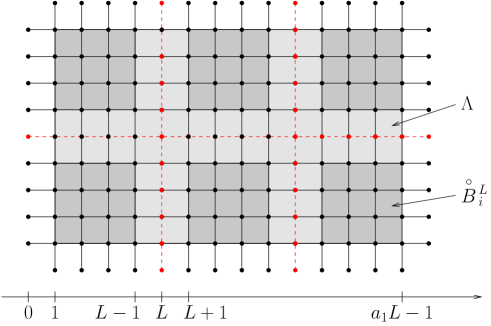
Figure 1: $E^{w}(\Lambda)$ partitioned into the ${\mathaccent 0{\accentclass@}017{E}^{L}_{i}}$ and the lateral (dashed) edges.

The first crucial feature of $\Psi^{L}_{\Lambda}$ is its product structure: under $\Psi^{L}_{\Lambda}$ the restriction of $(J,\omega)$ to any ${\mathaccent 0{\accentclass@}017{E}^{L}_{i}}$ with $i\in I_{\Lambda,L}$ or to $\{e\}$ with $e\in E_{\operatorname{lat}}^{L}(\Lambda)$ is independent of the rest of the configuration, so that in particular the restriction of $\omega$ to $E^{L}_{i}$ is independent of its restriction to $\bigcup_{j\in I_{\Lambda,L}:\|j-i\|_{2}>1}E^{L}_{j}$, and for any $L$-connecting family point (ii) of Theorem 3.1 is verified.

The second essential property of $\Psi^{L}_{\Lambda}$ is that it is stochastically smaller than the averaged measure on $\Lambda$ with free boundary condition, namely point (i) of Theorem 3.1 is true. This is an immediate consequence of the following Proposition:

Proposition 3.2

Consider a finite edge set $E$ and a partition $(E_{i})_{i=1\ldots n}$ of $E$. Assume that $h:\mathcal{J}\times\Omega\rightarrow\mathbb{R}$ is $\mathcal{B}_{E}$-measurable in the first variable and that for every $J$, $h(J,.)$ is an increasing function. If we denote by $(J_{i},\omega_{i})\in\mathcal{J}_{E_{i}}\times\Omega_{E_{i}}$ the variables associated to the measure $\mathbb{E}\Phi_{E_{i}}^{J_{i},f}$ (resp. $\mathbb{E}\Phi_{E_{i}}^{J_{i},w}$), we have:

$$\mathbb{E}\Phi^{J,w}_{E}h \leqslant\left[\bigotimes_{i=1}^{n}\mathbb{E}_{E_{i}}\Phi_{E_{i}}^{J_{i},w}\right]\left(h(J_{1}\vee\ldots\vee J_{n},\omega_{1}\vee\ldots\vee\omega_{n})\right)$$ (22)

$$\mbox{resp. \ \ \ }\mathbb{E}\Phi^{J,f}_{E}h \geqslant\left[\bigotimes_{i=1}^{n}\mathbb{E}_{E_{i}}\Phi_{E_{i}}^{J_{i},f}\right]\left(h(J_{1}\vee\ldots\vee J_{n},\omega_{1}\vee\ldots\vee\omega_{n})\right).$$ (23)

[Proof.] We focus on the proof of the second inequality since both proofs are similar. We begin with the case $n=2$. Applying twice the DLR equation (6) for $\Phi$ we get, for any $J\in\mathcal{J}$:

$$\Phi^{J,f}_{E}\left(h(J,\omega)\right)=\Phi^{J,f}_{E}\left[\Phi^{J,\omega_{|E_{2}}}_{E_{1}}\left[\Phi^{J,\omega_{1}}_{E_{2}}\left(h\left(J,\omega_{1}\vee\omega_{2}\right)\right)\right]\right]$$

where $\omega$ is the variable for $\Phi^{J,f}_{E}$, $\omega_{1}$ that for $\Phi^{J,\omega_{|E_{2}}}_{E_{1}}$ and $\omega_{2}$ that for $\Phi^{J,\omega_{1}}_{E_{2}}$. Since $h\left(J,\omega_{1}\vee\omega_{2}\right)$ is an increasing function of $\omega_{1}$ and $\omega_{2}$, it is enough to use the monotonicity (8) of $\Phi^{J,\pi}_{E}$ along $\pi$ to conclude that

$$\Phi^{J,f}_{E}\left(h(J,\omega)\right)\geqslant\Phi^{J,f}_{E_{1}}\left[\Phi^{J,f}_{E_{2}}\left(h\left(J,\omega_{1}\vee\omega_{2}\right)\right)\right].$$

The same question on the $J$-variable is trivial since $\mathbb{P}$ is a product measure, namely if $J,J_{1},J_{2}$ are the variables corresponding to $\mathbb{E}_{E},\mathbb{E}_{E_{1}}$ and $\mathbb{E}_{E_{2}}$:

$$\mathbb{E}_{E}\Phi^{J,f}_{E}\left(h(J,\omega)\right)\geqslant\mathbb{E}_{E_{1}}\mathbb{E}_{E_{2}}\Phi^{J_{1},f}_{E_{1}}\left[\Phi^{J_{2},f}_{E_{2}}\left(h\left(J_{1}\vee J_{2},\omega_{1}\vee\omega_{2}\right)\right)\right].$$

It is clear that $\mathbb{E}_{E_{2}}$ and $\Phi^{J_{1},f}_{E_{1}}$ commute, and that $\mathbb{E}_{E_{1}}\Phi^{J_{1},f}_{E_{1}}$ and $\mathbb{E}_{E_{2}}\Phi^{J_{2},f}_{E_{2}}$ also commute, hence the claim is proved for $n=2$. We end the proof with the induction step, assuming that (23) holds for $n$ and that $E$ is partitioned into $(E_{i})_{i=1\ldots n+1}$. Applying the inductive hypothesis at rank $2$ to $E_{1}$ and $E^{\prime}_{2}=\cup_{i\geqslant 2}E_{i}$ we see that $\mathbb{E}\Phi^{J,f}_{E}h(J,\omega)\geqslant\mathbb{E}_{E_{1}}\Phi^{J_{1},f}_{E_{1}}\mathbb{E}_{E_{2}^{\prime}}\Phi^{J_{2}^{\prime},f}_{E_{2}^{\prime}}h\left(J_{1}\vee J_{2}^{\prime},\omega_{1}\vee\omega^{\prime}_{2}\right)$. Remarking that for any fixed $(J_{1},\omega_{1})$ the function $\left(J,\omega\right)\in\mathcal{J}\times\Omega\mapsto h(J_{1}\vee J_{|E^{\prime}_{2}},\omega_{1}\vee\omega)$ is $\mathcal{B}_{E^{\prime}_{2}}$-measurable in $J$ and increases with $\omega$ we can apply the inductive hypothesis at rank $n$ in order to expand further on $J^{\prime}_{2}$ and $\omega^{\prime}_{2}$ and the proof is over.

3.2 The $L$-connecting family $\mathcal{E}^{L,H}_{i}$

The second step towards the proof of Theorem 3.1 is the construction of a $L$-connecting family. The faces of the blocks $B^{L}_{i}$ play an important role hence we continue with some more notations. Remark that $(\kappa,\varepsilon)\in\{1,\ldots,d\}\times\{0,1\}$ indexes conveniently the $2d$ faces of $B^{L}_{i}$ if to $(\kappa,\varepsilon)$ we associate the face $Li+L\varepsilon\mathbf{e}_{\kappa}+\mathcal{F}^{L}_{\kappa}$ where

$$\mathcal{F}^{L}_{\kappa}=\{0,\ldots,L\}^{d}\cap\{x\cdot\mathbf{e}_{\kappa}=0\}.$$ (24)

We decompose then each of these faces into smaller $d-1$ dimensional hypercubes and let

$$\mathcal{H}^{L,H}_{\kappa}=\left\{j\in\mathbb{Z}^{d}:\begin{array}[]{l}j\cdot\mathbf{e}_{\kappa}=0\mbox{ and }\forall k\in\{1,\ldots,d\}\setminus\{\kappa\},\\ L/({3H})\leqslant j\cdot\mathbf{e}_{k}\leqslant{2L}/({3H})-1\end{array}\right\}$$ (25)

and for any $j\in\mathcal{H}^{L,H}_{\kappa}$ we denote

$$F^{L,H}_{i,\kappa,\varepsilon,j}=Li+L\varepsilon\mathbf{e}_{\kappa}+Hj+\mathcal{F}^{H-1}_{\kappa}$$ (26)

so that $F^{L,H}_{i,\kappa,\varepsilon,j}$ is the translated of $\mathcal{F}^{H-1}_{\kappa}$ positioned at $Hj$ on the face $(\kappa,\varepsilon)$ of $B^{L}_{i}$, as illustrated on Figure 2.

Figure 2: The $d-1$ dimensional facets $F^{L,H}_{i,\kappa,\varepsilon,j}$.

The facets $F^{L,H}_{i,\kappa,\varepsilon,j}$ will play the role of seeds for the $L$-connecting family. Given $\omega\in\Omega_{E^{w}(\Lambda)}$ and $i\in I_{\Lambda,L}$, $(\kappa,\varepsilon)\in\{1,\ldots,d\}\times\{0,1\}$ and $j_{0}\in\mathcal{H}^{L,H}_{\kappa}$, we say that $F^{L,H}_{i,\kappa,\varepsilon,j_{0}}$ is a seed at scale $H$ for the face $(\kappa,\varepsilon)$ of $B^{L}_{i}$ if $j_{0}$ is the smallest index in the lexicographical order among the $j\in\mathcal{H}^{L,H}_{\kappa}$ such that either $F^{L,H}_{i,\kappa,\varepsilon,j}\cap\Lambda=\emptyset$, or all the edges $e\in E^{f}(F^{L,H}_{i,\kappa,\varepsilon,j})$ are open for $\omega$ (we recall that $E^{f}(\Lambda^{\prime})$ is the set of edges between any two adjacent points of $\Lambda^{\prime}\subset\mathbb{Z}^{d}$, cf. (3))

The first condition is designed to handle the case when the face $(\kappa,\varepsilon)$ of $B^{L}_{i}$ is not in $\Lambda$ (this happens if ${\mathaccent 0{\accentclass@}017{B}^{L}_{i}}$ touches the border of $\Lambda$, cf. Figure 1): with our conventions, there always exists a seed in that case and it is the $F^{L,H}_{i,\kappa,\varepsilon,j}$ of smallest index $j\in\mathcal{H}^{L,H}_{\kappa}$.

Then, we let

$$\mathcal{E}^{L,H}_{i}=\left\{\omega\in\Omega_{E^{w}(\Lambda)}:\mbox{\begin{tabular}[]{l}Each face of $B^{L}_{i}$ owns a seed and\\ these are connected under $\omega_{|E^{L}_{i}}$\end{tabular}}\right\},\forall i\in I_{\Lambda,L}$$ (27)

which is clearly a $L$-connecting family since, on the one hand, $\mathcal{E}^{L,H}_{i}$ depends on $\omega_{|E^{L}_{i}}$ only and, on the second hand, the seed on the face $(\kappa,1)$ of $B^{L}_{i}$ corresponds by construction to that on the face $(\kappa,0)$ of $B^{L}_{i+\mathbf{e}_{\kappa}}$, for any $i,i+\mathbf{e}_{\kappa}\in I_{\Lambda,L}$. Hence we are left with the proof of part (iii) of Theorem 3.1.

3.3 Large probability for $\mathcal{E}^{L}_{i}$ under $\Psi^{L}_{\Lambda}$

In this Section we conclude the proof of Theorem 3.1 with an estimate over the $\Psi^{L}_{\Lambda}$-probability of

$$\mathcal{E}^{L}_{i}=\mathcal{E}^{L,[\sqrt[d]{\delta\log L}]}_{i}$$ (28)

for $\delta>0$ small enough, and show as required that $\Psi^{L}_{\Lambda}(\mathcal{E}^{L}_{i})\rightarrow 1$ as $L\rightarrow\infty$ assuming (SP, $d\geqslant 3$), uniformly over $\Lambda$ and $i\in I_{\Lambda,L}$. Our proof is made of the two Lemmas below: first we prove the existence of seeds with large probability and then we estimate the conditional probability for connecting them.

Lemma 3.3

Assume that $c=\mathbb{E}\Phi^{J,f}_{\{e\}}(\omega_{e})>0$ and let $\delta<-1/\log c$. Then there exists $(\rho_{L})_{L\geqslant 3}$ with $\lim_{L\rightarrow\infty}\rho_{L}=1$ such that, for every $L$-admissible $\Lambda$ and every $i\in I_{\Lambda,L}$,

$$\Psi^{L}_{\Lambda}\left(\left\{\mbox{Each face of $B^{L}_{i}$ bears a seed at scale }H_{L}=[\sqrt[d]{\delta\log L}]\right\}\right)\geqslant\rho_{L}.$$

Lemma 3.4

Assume (SP, $d\geqslant 3$). Then, there exists $(\rho^{\prime}_{H})_{H\in\mathbb{N}^{\star}}$ with $\rho^{\prime}_{H}\rightarrow 1$ as $H\rightarrow\infty$ such that, for any $L\in\mathbb{N}^{\star}$ such that $\mathcal{H}^{L,H}_{1}\neq\emptyset$, any $L$-admissible domain $\Lambda\subset\mathbb{Z}^{d}$ and any $i\in I_{\Lambda,L}$,

$$\Psi^{L}_{\Lambda}\left(\mathcal{E}_{i}^{L,H}\left|\left\{\mbox{\begin{tabular}[]{l}Each face of $B^{L}_{i}$ bears\\ a seed at scale $H$\end{tabular}}\right.\right\}\right)\geqslant\rho^{\prime}_{H}.$$ (29)

Before proving Lemmas 3.3 and 3.4 we state an important warning: the fact that $\Psi^{L}_{\Lambda}(\mathcal{E}^{L}_{i})\rightarrow 1$ as $L\rightarrow\infty$ does not give any information on the probability of $\mathcal{E}_{i}^{L}$ under the averaged measure $\mathbb{E}\Phi^{J}_{\Lambda}$ as $\mathcal{E}^{L}_{i}$ is not an increasing event !

[Proof.] (Lemma 3.3). The $\Psi^{L}_{\Lambda}$-probability for any lateral edge of $B^{L}_{i}$ to be open equals $c$, hence a facet $F^{L,H_{L}}_{i,\kappa,\varepsilon,j}\subset\Lambda$ is entirely open with a probability

$$c^{(d-1)(H_{L}-1)H_{L}^{d-2}}\geqslant c^{H_{L}^{d}}$$

for $L$ large enough. Consequently, the probability that there is a seed at scale $H_{L}$ on each face of $B^{L}_{i}$ is at least

$$\rho_{L} =1-2d\left(1-c^{H_{L}^{d}}\right)^{\left[\frac{L}{3H_{L}}-2\right]^{d-1}}$$

$$\geqslant 1-2d\exp\left(-c^{H_{L}^{d}}\times\left[\frac{L}{3H_{L}}-2\right]^{d-1}\right)$$ (30)

using the inequality $1-u\leqslant\exp\left(-u\right)$. We remark at last that for $L$ large,

$$\log\left(c^{H_{L}^{d}}\times\left[\frac{L}{3H_{L}}-2\right]^{d-1}\right) \geqslant H_{L}^{d}\log c+(d-1)\left(\log L-\log(4H_{L})\right)$$

$$\geqslant\left(1+\delta\log c\right)\log L-\log(4H_{L})$$

with $1+\delta\log c>0$ thanks to the assumption on $\delta$, hence the term in the exponential in (30) goes to $-\infty$ as $L\rightarrow\infty$ and we have proved that $\lim_{L\rightarrow\infty}\rho_{L}=1$.

[Proof.] (Lemma 3.4). We fix a realization ${\omega_{\operatorname{ext}}}\in\Omega_{E^{w}(\Lambda)\setminus{\mathaccent 0{\accentclass@}017{E}^{L}_{i}}}$ such that each face of $B^{L}_{i}$ bears a seed under ${\omega_{\operatorname{ext}}}$. Thanks to the product structure of $\Psi^{L}_{\Lambda}$, the restriction to ${\mathaccent 0{\accentclass@}017{E}^{L}_{i}}$ of the conditional measure $\Psi^{L}_{\Lambda}\left(.|\omega={\omega_{\operatorname{ext}}}\right)$ equals $\mathbb{E}\Phi^{J,f}_{{\mathaccent 0{\accentclass@}017{E}^{L}_{i}}}$, hence the probability for connecting all seeds together is

$$\mathbb{E}\Phi^{J,f}_{{\mathaccent 0{\accentclass@}017{E}^{L}_{i}}}\left(\omega\vee{\omega_{\operatorname{ext}}}\in\mathcal{E}^{L,H}_{i}\right).$$

We will prove below that with large probability one can connect a seed to the seed in any adjacent face, and this will be enough for concluding the proof. Indeed, denote $s_{1},\ldots,s_{2d}$ the seeds of ${\omega_{\operatorname{ext}}}$. Thanks to the requirement $a_{i}\geqslant 2$ in the definition of $L$-admissible sets, we can assume that $s_{1}$ and $s_{2}$ are on adjacent faces, both of them inside $\Lambda$ so that in fact $s_{1}$ and $s_{2}$ are entirely open for ${\omega_{\operatorname{ext}}}$. If we connect $s_{1}$ to each of the seeds $s_{2},\ldots,s_{2d-1}$ in the adjacent faces of $B^{L}_{i}$, and then in turn connect $s_{2}$ to $s_{2d}$ we have connected all seeds together. As a consequence one can take

$$\rho^{\prime}_{H}=1-(2d-1)(1-\inf_{L:\mathcal{H}^{L,H}_{1}\neq\emptyset}\rho^{\prime\prime}_{H,L})$$ (31)

as a lower bound in (29), where $\rho^{\prime\prime}_{H,L}$ is the least probability under $\mathbb{E}\Phi^{J,f}_{{\mathaccent 0{\accentclass@}017{E}^{L}_{i}}}$ for connecting two facets $F^{L,H}_{i,\kappa,\varepsilon,j}$ and $F^{L,H}_{i,\kappa^{\prime},\varepsilon^{\prime},j^{\prime}}$ in adjacent faces of $B^{L}_{i}$.

For the sake of simplicity we let $i=0$, $(\kappa,\varepsilon)=(1,0)$ and $(\kappa^{\prime},\varepsilon^{\prime})=(2,0)$. Our objective is to connect any two facets $F^{L,H}_{0,1,0,j}$ and $F^{L,H}_{0,2,0,j^{\prime}}$ ($j\in\mathcal{H}^{L,H}_{1}$ and $j^{\prime}\in\mathcal{H}^{L,H}_{2}$) with large probability under $\mathbb{E}\Phi^{J,f}_{{\mathaccent 0{\accentclass@}017{B}^{L}_{0}}}$, and we achieve this placing slabs in $B^{L}_{0}$. Thanks to assumption (SP, $d\geqslant 3$) there exist $\alpha>0$ and $H_{s}\in\mathbb{N}^{\star}$ such that any two points in $S\cup\partial S$ are connected by $\omega$ with probability at least $\alpha$ under $\mathbb{E}\Phi^{J,f}_{S}$, provided that $S$ is of the form $S=\{1,\ldots,N-1\}^{d-1}\times\{1,H_{s}-1\}$ with $N\in\mathbb{N}$ large enough. We describe now two sequences of slabs of height $H_{s}$ linking the seeds $F^{L,H}_{0,1,0,j}$ and $F^{L,H}_{0,2,0,j^{\prime}}$ to each other. Let first, for $l\in\mathbb{N}$ and $\kappa\in\{1,2\}$:

$$S(l,\kappa)=\{1,\ldots,l-1\}^{d}\cap\{x:1\leqslant x\cdot\mathbf{e}_{\kappa}\leqslant H_{s}-1\}$$ (32)

and then

$$U(l,h,\kappa)=S(l,\kappa)+h\mathbf{e}_{\kappa}+\sum_{k\geqslant 3}\left[\frac{L-l}{2}\right]\mathbf{e}_{k}$$ (33)

for $l\in\{1,\ldots,L\}$, $h\in\{0,\ldots,L-H_{s}\}$ and $\kappa\in\{1,2\}$. The slab $U(l,h,\kappa)$ is normal to $\mathbf{e}_{\kappa}$ and the $\mathbf{e}_{\kappa}$-coordinates of its points remain in $\{h+1,\ldots,h+H_{s}-1\}$, it is in contact with the face $(\kappa^{\prime},0)$ of ${\mathaccent 0{\accentclass@}017{B}^{L}_{0}}$ where $\{\kappa^{\prime}\}=\{1,2\}\setminus\{\kappa\}$ and it is positioned roughly at the center of ${\mathaccent 0{\accentclass@}017{B}^{L}_{i}}$ in every other direction $\mathbf{e}_{k}$ for $k\geqslant 3$. We conclude these geometrical definitions letting

$$V_{n}=U\left(j\cdot\mathbf{e}_{2}H+(n-1)H_{s},j^{\prime}\cdot\mathbf{e}_{1}H+(n-1)H_{s},1\right)$$ (34)

which are vertical slabs and

$$T_{n}=U\left(j^{\prime}\cdot\mathbf{e}_{1}H+nH_{s},j\cdot\mathbf{e}_{2}H+(n-1)H_{s},2\right)$$ (35)

which are horizontal slabs, for any $n\in\{1,\ldots,\lceil H/H_{s}\rceil\}$. As illustrated on Figure 3, for any $n\in\{1,\ldots,\lceil H/H_{s}\rceil\}$, $F^{L,H}_{0,1,0,j}$ is in contact with $E^{w}(T_{n})$ since the largest dimension of the slab is at least $L/3$, while $E^{w}(V_{n})$ touches $F^{L,H}_{0,2,0,j^{\prime}}$, and by construction $E^{w}(V_{n})$ and $E^{w}(T_{n})$ touch each other. Furthermore the edge sets $E^{w}(V_{n})$ and $E^{w}(T_{n})$ are all disjoint, and all included in $E^{w}({\mathaccent 0{\accentclass@}017{B}^{L}_{0}})$. Consider now the product measure

$$\Theta=\bigotimes_{n=1}^{\lceil H/H_{s}\rceil}\left(\mathbb{E}\Phi^{J,f}_{V_{n}}\otimes\mathbb{E}\Phi^{J,f}_{T_{n}}\right).$$ (36)

Under the measure $\Theta$, the probability that there is a $\omega$-open path in $E^{w}(V_{n})\cup E^{w}(T_{n})$ between the two seeds $F^{L,H}_{0,1,0,j}$ and $F^{L,H}_{0,2,0,j^{\prime}}$ is at least $\alpha^{2}$ thanks to (SP, $d\geqslant 3$). By independence of the restrictions of $\omega$ to the unions of slabs $\left(E^{w}(V_{n})\cup E^{w}(T_{n})\right)_{n=1\ldots\lceil H/H_{s}\rceil}$, it follows that the $\Theta$-probability that $\omega$ does not connect $F^{L,H}_{0,1,0,j}$ to $F^{L,H}_{0,2,0,j^{\prime}}$ in $E^{w}({\mathaccent 0{\accentclass@}017{B}^{L}_{0}})$ is not larger than $\left(1-\alpha^{2}\right)^{\lceil H/H_{s}\rceil}$. Thanks to the stochastic domination $\Theta\underset{stoch.}{\leqslant}\mathbb{E}\Phi^{J,f}_{{\mathaccent 0{\accentclass@}017{B}^{L}_{0}}}$ seen in Proposition 3.2, the same control holds for the measure $\mathbb{E}\Phi^{J,f}_{{\mathaccent 0{\accentclass@}017{B}^{L}_{0}}}$ and we have proved that

$$\rho^{\prime\prime}_{H,L}\geqslant\left(1-\alpha^{2}\right)^{\lceil H/H_{s}\rceil}$$

for any $L$ such that $\mathcal{H}^{L,H}_{1}\neq\emptyset$. In view of (31) this yields $\lim_{H\rightarrow\infty}\rho^{\prime}_{H}=1$.

Figure 3: The slabs $V_{n}$ and $T_{n}$ in the proof of Lemma 3.4.

3.4 Existence of a crossing cluster

An easy consequence of Theorem 3.1 is the following:

Corollary 3.5

If (SP, $d\geqslant 3$), for any $L\in\mathbb{N}^{\star}$ large enough one has

$$\lim_{N}\mathbb{E}\Phi^{J,f}_{\Lambda_{LN}}\left(\mbox{There exists a crossing cluster for }\omega\mbox{ in }\Lambda_{LN}\right)=1.$$

[Proof.] The existence of a crossing cluster is an increasing event hence it is enough to prove the estimate under the stochastically smaller measure $\Psi^{L}_{\Lambda_{LN}}$. Under $\Psi^{L}_{\Lambda_{LN}}$ the events $\mathcal{E}_{i}^{L}$ are only $1$-dependent thus for $L$ large enough the collection $(\mathbf{1}_{\{\mathcal{E}_{i}^{L}\}})_{i\in I_{\Lambda,L}}$ stochastically dominates a site percolation process with high density [25]. In particular, the coarse graining [29] yields the existence of a crossing cluster for $(\mathbf{1}_{\{\mathcal{E}_{i}^{L}\}})_{i\in I_{\Lambda,L}}$ in $I_{\Lambda,L}$ with large probability as $N\rightarrow\infty$, and the latter event implies the existence of a crossing cluster for $\omega$ in $\Lambda_{LN}$ as $(\mathcal{E}_{i}^{L})_{i\in I_{\Lambda,L}}$ is a $L$-connecting family.

4 Uniqueness of large clusters

In the previous Section we established Theorem 3.1, that gives a first description of the behavior of clusters in a large box. Our present objective is to use that information in order to infer from the slab percolation assumption (SP, $d\geqslant 3$) a uniform slab percolation criterion (USP).

Given $L,n\in\mathbb{N}^{\star}$ with $n\geqslant 3$ we let

$$\Lambda_{n,L}^{\log}=\{1,Ln-1\}^{d-1}\times\{1,L\lceil\log n\rceil-1\},$$ (37)

call ${\mathrm{Bottom}}(\Lambda^{\log}_{n,L})=\{1,\ldots,Ln-1\}^{d-1}\times\{0\}$ and ${\mathrm{Top}}(\Lambda^{\log}_{n,L})=\{1,\ldots,Ln-1\}^{d-1}\times\{L\lceil\log n\rceil\}$ the horizontal faces of $\partial\Lambda_{n,L}^{\log}$, consider $o=(1,\ldots,1,1)\in\mathbb{Z}^{d}$ a reference point in $\Lambda_{n,L}^{\log}$ and $\mathbb{H}^{-}$ the discrete lower half space

$$\mathbb{H}^{-}=\{x\in\mathbb{Z}^{d}:x\cdot\mathbf{e}_{d}\leqslant 0\}.$$ (38)

as well as $E^{-}=E^{f}(\mathbb{H}^{-})$ the set of edges with all extremities in $\mathbb{H}^{-}$. Then, we define (USP) as follows:

$$\exists L\in\mathbb{N}^{\star},\exists\varepsilon>0\mbox{ such that for any $n$ large enough,}$$

$$\mathbb{P}\left(\begin{array}[]{l}\forall x\in{\mathrm{Bottom}}(\Lambda^{\log}_{n,L}),\forall\pi\in\Omega_{E^{w}(\Lambda^{\log}_{n,L})^{c}},\forall\xi\in\Omega_{E^{-}}:\\ \Phi_{\Lambda^{\log}_{n,L}}^{J,\pi}\left(x\stackrel{{\scriptstyle\omega\vee\xi}}{{\leftrightarrow}}o\mbox{ or }x\stackrel{{\scriptstyle\omega\vee\xi}}{{\nleftrightarrow}}{\mathrm{Top}}(\Lambda^{\log}_{n,L})\right)\geqslant\varepsilon\end{array}\right)\geqslant\varepsilon.$$ (USP)

The implication (SP, $d\geqslant 3$)$\Rightarrow$(USP) will be finally proved in Proposition 4.7, and its consequence – the uniqueness of large clusters – detailed in Proposition 4.9.

4.1 Typical structure in slabs of logarithmic height

As a first step towards the proof of the implication (SP, $d\geqslant 3$)$\Rightarrow$(USP) we work on the proof of Proposition 4.1 below. We need still a few more definitions. On the one hand, given $\omega\in\Omega$ and $x\in\mathbb{Z}^{d}$ we say that $o$ and $x$ are doubly connected under $\omega$ if there exist two $\omega$-open paths from $o$ to $x$ made of disjoint edges, and consider

$$\mathcal{C}^{2}_{o}\left(\omega\right)=\{x\in\mathbb{Z}^{d}:x\mbox{ is doubly connected to }o\mbox{ under }\omega\}.$$ (41)

On the second hand we describe the typical $J$-structure in order to permit local surgery on $\omega$ later on. Given a rectangular parallelepiped $\Lambda\subset\mathbb{Z}^{d}$ that is $L$-admissible, we generalize the notation $B^{L}_{i}$ defining

$$B^{L,n}_{i}=\left(Li+\{-nL+1,\ldots,(n+1)L-1\}^{d}\right)\cap\Lambda$$ (42)

for $n\in\mathbb{N}$; note that ${\mathaccent 0{\accentclass@}017{B}^{L}_{i}}=B_{i}^{L,0}$ if $i\in I_{\Lambda,L}$ (see (19)). Given $J\in\mathcal{J}$ and $e\in E(\mathbb{Z}^{d})$, we say that $e$ is $J$-open if $J_{e}>0$. For all $i\in I_{\Lambda,L}$ we denote

$$\mathcal{G}_{i}^{L}=\left\{\begin{array}[]{l}\mbox{There exists a unique $J$-open cluster in}\\ E^{w}(B^{L,1}_{i})\mbox{ of diameter larger or equal to $L$}\\ \mbox{and }\forall e\in E^{w}(B_{i}^{L,3}),J_{e}=0\mbox{ or }J_{e}\geqslant\varepsilon_{L}\end{array}\right\}$$ (43)

where $\varepsilon_{L}>0$ is a cutoff that satisfies $\mathbb{P}\left(0<J_{e}<\varepsilon_{L}\right)\leqslant e^{-L}$. Given a finite rectangular parallelepiped $R\subset\mathbb{Z}^{d}$ and $I\subset\mathbb{Z}^{d}$ we say that $I$ presents an horizontal interface in $R$ if there exists no $\ast$-connected path $c_{1},\ldots,c_{n}$ (i.e. $\|c_{i+1}-c_{i}\|_{\infty}=1$, $\forall i=1\ldots n-1$) in $R\setminus I$ with $c_{1}\cdot\mathbf{e}_{d}=\min_{x\in R}x\cdot\mathbf{e}_{d}$ and $c_{n}\cdot\mathbf{e}_{d}=\max_{x\in R}x\cdot\mathbf{e}_{d}$. We consider at last the event

$$\mathcal{L}=\left\{(J,\omega):\begin{array}[]{l}\mbox{There exists an horizontal interface }\mathcal{I}\mbox{ in}\\ \{0,\ldots,n-1\}^{d-1}\times\left\{1,\ldots,\lceil\log n\rceil-1\right\}\mbox{ such }\\ \mbox{that: }\forall i\in\mathcal{I}\mbox{, }\mathcal{C}^{2}_{o}\left(\omega\right)\cap B^{L}_{i}\neq\emptyset\mbox{ and }J\in\mathcal{G}^{L}_{i}\end{array}\right\}$$ (44)

and claim:

Proposition 4.1

(SP, $d\geqslant 3$) implies the existence of $L\in\mathbb{N}^{\star}$ such that

$$\liminf_{n\rightarrow\infty}\mathbb{E}\inf_{\pi}\Phi_{\Lambda_{n,L}^{\log}}^{J,\pi}\left(\mathcal{L}\right)>0.$$

The proof of this Proposition is not straightforward and we achieve first several intermediary estimates under the product measure $\Psi^{L/3}_{\Lambda^{\log}_{n,L}}$.

4.1.1 Double connections

The event $\mathcal{E}^{L}_{i}$ introduced in the former Section efficiently describes connections between sub-blocks in the domain $\Lambda$. However, as it will appear in the proof of Proposition 4.7, the information provided by $\mathcal{E}^{L}_{i}$ is not enough to be able to proceed to local modifications on $\omega$ in a recognizable way and this is the motivation for introducing the notion of double connections. Assuming that $L$ is a multiple of $3$, that $\Lambda\subset\mathbb{Z}^{d}$ is a $L$-admissible domain and that $i\in I_{\Lambda,L}$ we define

$$\mathcal{D}^{L}_{i}=\bigcap_{j\in 3i+\{0,1,2\}^{d}}\mathcal{E}_{j}^{L/3}.$$ (45)

Note that $\mathcal{D}^{L}_{i}$ depends on $\omega$ in $E^{L}_{i}$, a box of side-length $L$, while the measure $\Psi^{L/3}_{\Lambda}$ associated to the $\mathcal{E}_{j}^{L/3}$ has a decorrelation length $L/3$.

An immediate consequence of Theorem 3.1 is the following fact:

Lemma 4.2

Assumption (SP, $d\geqslant 3$) implies:

$$\lim_{L\rightarrow\infty,3|L}\inf_{\mbox{\scriptsize{$\begin{array}[]{c}\Lambda\subset\mathbb{Z}^{d}L\mbox{-admissible}\\ i\in I_{\Lambda,L}\end{array}$}}}\Psi^{L/3}_{\Lambda}\left(\mathcal{D}^{L}_{i}\right)=1.$$

Moreover, the event $\mathcal{D}^{L}_{i}$ depends only on $\omega_{|E^{L}_{i}}$. For any $i,j\in I_{\Lambda,L}$ with $\|i-j\|_{2}>1$ the events $\mathcal{D}^{L}_{i}$ and $\mathcal{D}^{L}_{j}$ are independent under $\Psi^{L/3}_{\Lambda}$.

The relation between $\mathcal{D}^{L}_{i}$ and the notion of double connections appears below:

Lemma 4.3

If $(i_{1},\ldots,i_{n})$ is a path in $\mathbb{Z}^{d}$ such that ${\mathaccent 0{\accentclass@}017{B}^{L}_{i_{k}}}\subset\Lambda,\forall k=1\ldots n$ and if $\omega\in\mathcal{D}_{i_{1}}^{L}\cap\ldots\cap\mathcal{D}_{i_{n}}^{L}$, then there exist $x\in B^{L}_{i_{1}}$ and $y\in B^{L}_{i_{n}}$ and two $\omega$-open paths from $x$ to $y$ in $\bigcup_{k=1}^{n}E^{L}_{i_{k}}$ made of distinct edges.

This fact is an immediate consequence of the properties of $\mathcal{E}_{j}^{L/3}$, see Figure 4. Note that the factor $3$ in $\mathcal{E}_{j}^{L/3}$ is necessary as the $\omega$-open clusters described by $\mathcal{E}_{j}^{L/3}$ may use the edges on the faces of $B_{j}^{L/3}$.

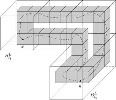
Figure 4: A loop made of good $\mathcal{E}^{L/3}$-blocks in a path of good $\mathcal{D}^{L}$-blocks.

4.1.2 Local $J$-structure

We describe now the typical $J$-structure with the help of the event $\mathcal{G}_{i}^{L}$ (see (43)).

Lemma 4.4

The event $\mathcal{G}_{i}^{L}$ depends only on $J_{|E^{w}(B^{L,3}_{i})}$, and (SP, $d\geqslant 3$) implies

$$\lim_{L\rightarrow\infty}\inf_{\mbox{\scriptsize{$\begin{array}[]{c}\Lambda\subset\mathbb{Z}^{d}L\mbox{-admissible}\\ i\in I_{\Lambda,L}\end{array}$}}}\Psi^{L/3}_{\Lambda}\left(\mathcal{G}^{L}_{i}\right)=1.$$

[Proof.] The domain of dependence of $\mathcal{G}_{i}^{L}$ is trivial. Concerning the estimate on its probability, we remark that the marginal on $J$ of $\Psi^{L/3}_{\Lambda}$ equals $\mathbb{P}$, while (SP, $d\geqslant 3$) ensures that percolation in slabs holds for the variable $\mathbf{1}_{\{J_{e}>0\}}$ under $\mathbb{P}$. Hence the condition on the structure of the $J$-open clusters holds with a probability larger than $1-e^{-cL}$ for some $c>0$ according to [29]. The condition on the value of $J_{e}$ also has a very large probability thanks to the choice of $\varepsilon_{L}$: remark that $|E^{w}(B_{i}^{L,3})|\leqslant d(7L)^{d}$, hence

$$\mathbb{P}\left(\exists e\in E^{w}\left(B_{i}^{L,3}\right):J_{e}\in(0,\varepsilon_{L})\right)\leqslant d(7L)^{d}e^{-L}$$

which goes to $0$ as $L\rightarrow\infty$.

4.1.3 Typical structure in logarithmic slabs

We proceed now with Peierls estimates in order to infer some controls on the global structure of $(J,\omega)$ in slabs of logarithmic height. We define

$$\mathcal{T}_{i}^{L}=\mathcal{D}^{L}_{i}\cap\mathcal{G}^{L}_{i}$$

where $\mathcal{D}^{L}_{i}$ and $\mathcal{G}^{L}_{i}$ are the events defined at (45) and (43) (see also (28) for the definition of $\mathcal{E}^{L}_{i}$). An immediate consequence of Lemmas 4.2 and 4.4 is that

$$\lim_{L\rightarrow\infty,3|L}\inf_{\mbox{\scriptsize{$\begin{array}[]{c}\Lambda\subset\mathbb{Z}^{d}L\mbox{-admissible}\\ i\in I_{\Lambda,L}\end{array}$}}}\Psi^{L/3}_{\Lambda}\left(\mathcal{T}^{L}_{i}\right)=1$$

if (SP, $d\geqslant 3$), together with the independence of $\mathcal{T}^{L}_{i}$ and $\mathcal{T}^{L}_{j}$ under $\Psi^{L/3}_{\Lambda}$ if $\|i-j\|_{\infty}\geqslant 7$. We recall the notation $\Lambda_{n,L}^{\log}=\{1,Ln-1\}^{d-1}\times\{1,L\lceil\log n\rceil-1\}$ (37) and claim:

Lemma 4.5

Assume (SP, $d\geqslant 3$). For any $\varepsilon>0$, $L$ large enough multiple of $3$,

$$\liminf_{n}\Psi_{\Lambda_{n,L}^{\log}}^{L/3}\left(\begin{array}[]{l}\mbox{The cluster of $\mathcal{T}_{i}^{L}$-good blocks issued}\\ \mbox{from $0$ presents an horizontal interface}\\ \mbox{in }\{0,n-1\}^{d}\times\{1,\lceil\log n\rceil-1\}\end{array}\right)\geqslant 1-\varepsilon.$$

Remark that the cluster of $\mathcal{T}_{i}^{L}$-good blocks issued from $0$ lives in $\{0,n-1\}^{d}\times\{\mathbf{0},\lceil\log n\rceil-1\}$, hence we require here (as in the definition of $\mathcal{L}$ at (44)) that the interface does not use the first layer of blocks. This is done in prevision for the proof of Lemma 4.6.

[Proof.] The proof is made of two Peierls estimates. A first estimate that we do not expand here permits to prove that some $\left(\mathcal{T}_{i}^{L}\right)$-cluster forms an horizontal interface with large probability in the desired region $\{0,\ldots,n-1\}^{d-1}\times\{1,\ldots,\lceil\log n\rceil-1\}$ if $L$ is large enough. The second estimate concerns the probability that there exists a $\mathcal{T}$-open path from $0$ to the top of the region.

If the $\mathcal{T}$-cluster issued from $0$ does not touch the top of the region, there exists a $\ast$-connected, self avoiding path of $\mathcal{T}$-closed sites in the vertical section $\left\{0,\ldots,n-1\right\}\times\{0\}^{d-2}\times\left\{0,\ldots,\lceil\log n\rceil-1\right\}$ separating $0$ from the top of the region. We call this event $\mathcal{C}$ and enumerate the possible paths according to their first coordinate on the left side $h\geqslant 0$ and their length $l\geqslant h+1$: there are not more than $7^{l}$ such paths. On the other hand, in any path of length $l$ we can select at least $\lceil l/13^{2}\rceil$ positions at $\|.\|_{\infty}$-distance at least $7$ from any other. As the corresponding $\mathcal{T}$-events are independent under $\Psi_{\Lambda_{n,L}^{\log}}^{L/3}$,

$$\Psi_{\Lambda_{n,L}^{\log}}^{L/3}\left(\mathcal{C}\right)\leqslant\sum_{h\geqslant 0}\sum_{l\geqslant h+1}7^{l}\left(1-\rho_{L}\right)^{l/13^{2}}$$

where $\rho_{L}=\inf_{i\in I_{\Lambda,L}}\Psi^{L/3}_{\Lambda}\left(\mathcal{T}^{L}_{i}\right)$. This is not larger than $a_{L}/(1-a_{L})^{2}$ if $a_{L}=7\left(1-\rho_{L}\right)^{1/13^{2}}<1$, and since $\lim_{L}a_{L}=0$ the claim follows.

4.1.4 Proof of Proposition 4.1

We conclude these intermediary estimates with the proof of Proposition 4.1. [Proof.](Proposition 4.1). As the event $\mathcal{L}$ is increasing in $\omega$, thanks to Proposition 3.2 it is enough to estimate its probability under the product measure $\Psi^{L/3}_{\Lambda_{n,L}^{\log}}$. We consider the following events on $(J,\omega)$:

$$A =\left\{\mbox{\begin{tabular}[]{l}$(J,\omega)$: there exists a modification of $(J,\omega)$ on $E^{w}({\mathaccent 0{\accentclass@}017{B}^{L}_{0}})$\\ such that the $\mathcal{T}$-cluster issued from $0$ forms an\\ horizontal interface in $\{0,\ldots,n-1\}^{d-1}\times\left\{1,\ldots,\lceil\log n\rceil-1\right\}$\end{tabular}}\right\}$$

$$B =\left\{\forall e\in E^{w}({\mathaccent 0{\accentclass@}017{B}^{L}_{0}}),J_{e}\geqslant\varepsilon_{L}\mbox{ and }\omega_{e}=1\right\}.$$

By a modification of $(J,\omega)$ on $E^{w}({\mathaccent 0{\accentclass@}017{B}^{L}_{0}})$ we mean a configuration $(J^{\prime},\omega^{\prime})\in\mathcal{J}\times\Omega$ that coincides with $(J,\omega)$ outside $E^{w}({\mathaccent 0{\accentclass@}017{B}^{L}_{0}})$. Clearly, the event $A$ does not depend on $(J,\omega)_{|E^{w}({\mathaccent 0{\accentclass@}017{B}^{L}_{0}})}$, whereas $B$ depends uniquely on $(J,\omega)_{|E^{w}({\mathaccent 0{\accentclass@}017{B}^{L}_{0}})}$. According to the product structure of $\Psi^{L/3}_{\Lambda^{\log}_{n,L}}$, we have

$$\Psi_{\Lambda_{n,L}^{\log}}^{L/3}\left(A\cap B\right)=\Psi_{\Lambda_{n,L}^{\log}}^{L/3}\left(A\right)\times\Psi_{{\mathaccent 0{\accentclass@}017{B}^{L}_{0}}}^{L/3}\left(B\right).$$

In view of Lemma 4.5, $\liminf_{n}\Psi_{\Lambda_{n,L}^{\log}}^{L/3}\left(A\right)\geqslant 1/2$ for $L$ large enough multiple of $3$, whereas $\Psi_{{\mathaccent 0{\accentclass@}017{B}^{L}_{0}}}^{L/3}\left(B\right)>0$ for any $L$ large enough (we just need $\mathbb{P}\left(J_{e}\geqslant\varepsilon_{L}\right)\geqslant\mathbb{P}\left(J_{e}>0\right)-e^{-L}>0$). This proves that $\liminf_{n}\Psi_{\Lambda_{n,L}^{\log}}^{L/3}\left(A\cap B\right)>0$ for $L$ large enough. We prove at last that $A\cap B$ is a subset of $\mathcal{L}$ and consider $(J,\omega)\in A\cap B$. From the definition of $A$ we know that there exists a modification $(J^{\prime},\omega^{\prime})$ of $(J,\omega)$ on $E^{w}({\mathaccent 0{\accentclass@}017{B}^{L}_{0}})$ such that the $\mathcal{T}$-cluster for $(J^{\prime},\omega^{\prime})$ issued from $0$ forms an horizontal interface in $\{0,\ldots,n-1\}^{d-1}\times\left\{1,\ldots,\lceil\log n\rceil-1\right\}$. Let us call $\mathcal{C}$ that $\mathcal{T}$-cluster and

$$\mathcal{I}=\mathcal{C}\cap\{0,\ldots,n-1\}^{d-1}\times\left\{1,\ldots,\lceil\log n\rceil-1\right\}.$$

From its definition it is clear that $\mathcal{I}$ contains an horizontal interface in $\{0,\ldots,n-1\}^{d-1}\times\left\{1,\ldots,\lceil\log n\rceil-1\right\}$; we must check now that $\forall i\in\mathcal{I},\mathcal{C}^{2}_{o}\left(\omega\right)\cap B^{L}_{i}\neq\emptyset$ and $J\in\mathcal{G}^{L}_{i}$. We begin with the proof that $\mathcal{C}^{2}_{o}\left(\omega\right)\cap B^{L}_{i}\neq\emptyset$, for every $i\in\mathcal{I}$: since $i\in\mathcal{C}$, Lemma 4.3 tells us that there exist $x\in{\mathaccent 0{\accentclass@}017{B}^{L}_{0}}$ and $y\in{\mathaccent 0{\accentclass@}017{B}^{L}_{i}}$ which are doubly connected under $\omega^{\prime}$. Since the corresponding paths enter at distinct positions in $E^{w}({\mathaccent 0{\accentclass@}017{B}^{L}_{0}})$, $y$ is also doubly connected to $o$ under $\omega$ which has all edges open in $E^{w}({\mathaccent 0{\accentclass@}017{B}^{L}_{0}})$. As for the $J$-structure, for every $i\in\mathcal{I}$ we have $(J^{\prime},\omega^{\prime})\in\mathcal{T}^{L}_{i}$, hence $J^{\prime}\in\mathcal{G}^{L}_{i}$ and $J\in\mathcal{G}^{L}_{i}$ for every $i\in\mathcal{I}$ such that ${\mathaccent 0{\accentclass@}017{B}^{L}_{0}}\cap B^{L,1}_{i}=\emptyset$. We conclude with the remark that the replacement of $J^{\prime}$ by $J$ in $E^{w}({\mathaccent 0{\accentclass@}017{B}^{L}_{0}})$ just enlarges an already large $J^{\prime}$-cluster (no new large cluster is created, hence $J^{\prime}\in\mathcal{G}^{L}_{i}\Rightarrow J\in\mathcal{G}^{L}_{i}$): the inclusion $(J^{\prime},\omega^{\prime})\in\mathcal{T}^{L}_{0}$ implies the existence of a $\omega^{\prime}$-open path of length $L$ in $E^{w}({\mathaccent 0{\accentclass@}017{B}^{L}_{0}})$, and this path is necessarily also $J^{\prime}$-open, hence $J\in\mathcal{G}^{L}_{i}$ for all $i\in\mathcal{I}$ such that ${\mathaccent 0{\accentclass@}017{B}^{L}_{0}}\cap B^{L,1}_{i}\neq\emptyset$, and this ends the proof that $A\cap B$ is a subset of $\mathcal{L}$.

4.2 First pivotal bond and local modifications

We introduce here the notion of first pivotal bond: given a configuration $\omega\in\Omega$, we call $\mathcal{C}^{2}_{x}(\omega)$ the set of points doubly connected to $x$ under $\omega$. Given $e\in E(\mathbb{Z}^{d})$ we say that $e$ is a pivotal bond between $x$ and $y$ under $\omega$ if $x\stackrel{{\scriptstyle\omega}}{{\leftrightarrow}}y$ in $\omega$ and $x\stackrel{{\scriptstyle\omega_{|\{e\}^{c}}}}{{\nleftrightarrow}}y$. At last we say that $e$ is the first pivotal bond from $x$ to $y$ under $\omega$ if it is a pivotal bond between $x$ and $y$ under $\omega$ and if it touches $\mathcal{C}^{2}_{x}\left(\omega\right)$.

There does not always exist a first pivotal bond between two connected points: it requires in particular the existence of a pivotal bond between these two points. When a first pivotal bond from $x$ to $y$ exists, it is unique. Indeed, assume by contradiction that $e\neq e^{\prime}$ are pivotal bonds under $\omega$ between $x$ and $y$ and that both of them touch $\mathcal{C}^{2}_{x}\left(\omega\right)$. If $c$ is an $\omega$-open path from $x$ to $y$, it must contain both $e$ and $e^{\prime}$. Assume that $c$ passes through $e$ before passing through $e^{\prime}$, then removing $e$ in $\omega$ we do not disconnect $x$ from $y$ since $e^{\prime}$ touches $\mathcal{C}^{2}_{x}\left(\omega\right)\supset\mathcal{C}_{x}\left(\omega_{|\{e\}^{c}}\right)$, and this contradicts the assumption that $e$ is a pivotal bond.

In the following geometrical Lemma we relate the event $\mathcal{L}$ defined at (44) to the notion of first pivotal bond. We recall the notations ${\mathrm{Bottom}}(\Lambda^{\log}_{n,L})=\{1,\ldots,Ln-1\}^{d-1}\times\{0\}$ and ${\mathrm{Top}}(\Lambda^{\log}_{n,L})=\{1,\ldots,Ln-1\}^{d-1}\times\{L\lceil\log n\rceil\}$, as well as $E^{-}$ for the set of edges in the discrete lower half space $\mathbb{H}^{-}$ (see (38)). We say that $\omega\in\Omega_{E}$ is compatible with $J\in\mathcal{J}_{E}$ if, for every $e\in E,J_{e}=0\Rightarrow\omega_{e}=0$.

Lemma 4.6

Consider $x\in{\mathrm{Bottom}}(\Lambda^{\log}_{n,L})$, $\xi\in\Omega_{E^{-}}$ and $(J,\omega)\in\mathcal{L}$ with $\omega$ such that

$$\mbox{$x\stackrel{{\scriptstyle\omega\vee\xi}}{{\leftrightarrow}}{\mathrm{Top}}(\Lambda^{\log}_{n,L})\mbox{ and }x\stackrel{{\scriptstyle\omega\vee\xi}}{{\nleftrightarrow}}o$}.$$

Then, there exists $i\in\{0,\ldots,n-1\}^{d-1}\times\{1,\ldots,\lceil\log n\rceil-1\}$ such that $J\in\mathcal{G}^{L}_{i}$ and there exists a modification $\omega^{\prime}$ of $\omega$ on $E^{w}(B^{L,1}_{i})$ compatible with $J$, such that the first pivotal bond from $o$ to $x$ under $\omega^{\prime}\vee\xi$ exists and belongs to $E^{w}(B^{L,1}_{i})$.

The variable $\xi$ corresponds to the configuration below the slab $\Lambda^{\log}_{n,L}$. The point in introducing $\xi$ here (and in the formulation of (USP)) is the need for an estimate that holds uniformly over the configuration below the slab in the proof of Lemma 4.8.

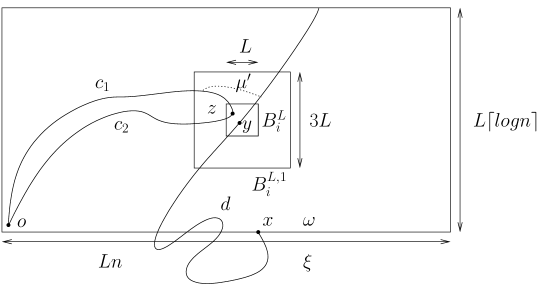
Figure 5: Lemma 4.6: $c_{1},c_{2}$ are $\omega$-open, $d$ is $\omega\vee\xi$-open and $\mu^{\prime}$ is $J$-open.

[Proof.] Note that Figure 5 provides an illustration for the objects considered in the proof. We build by hand the modification $\omega^{\prime}$. Since $(J,\omega)\in\mathcal{L}$ there exists an horizontal interface $\mathcal{I}$ as in (44). Since on the other hand $x\stackrel{{\scriptstyle\omega\vee\xi}}{{\leftrightarrow}}{\mathrm{Top}}(\Lambda^{\log}_{n,L})$, there exists $i\in\mathcal{I}$ such that $\mathcal{C}_{x}(\omega\vee\xi)\cap B^{L}_{i}\neq\emptyset$. Let us fix such an $i$: we clearly have $J\in\mathcal{G}^{L}_{i}$. From the definition of the event $\mathcal{L}$, we know that $\mathcal{C}^{2}_{o}(\omega)\cap B^{L}_{i}\neq\emptyset$. We fix $y\in\mathcal{C}_{x}(\omega\vee\xi)\cap B^{L}_{i}$ and $z\in\mathcal{C}^{2}_{o}(\omega)\cap B^{L}_{i}$. There exist two $\omega$-open paths $c_{1},c_{2}$ in $E^{w}(\Lambda_{n,L}^{\log})$ made of disjoint edges, with no loop, that link $o$ to $z$, as well as an $\omega\vee\xi$-open path $d$ in $E^{w}(\Lambda^{\log}_{n,L})\cup E^{-}$, with no loop, that links $x$ to $y$. Of course, $d$ does not touch $c_{1}\cup c_{2}$ since $x\nleftrightarrow o$ under $\omega\vee\xi$.

Since $i$ is not in the first block layer (see the remark after Lemma 4.5), $c_{1}\cap E^{w}(B^{L,1}_{i})$ and $d\cap E^{w}(B^{L,1}_{i})$ have a connected component of diameter larger or equal to $L$. Since $\mathbf{1}_{J_{e}>0}$ is larger than $\omega$ these components are also $J$-open, and since $J\in\mathcal{G}^{L}_{i}$, this implies that there exists a $J$-open path $\mu$ in $E^{w}(B^{L,1}_{i})$, self-avoiding, joining $c_{1}$ to $d$. Noting $(\mu_{t})_{t}$ the vertices of $\mu$, we call $v=\min\{t:\mu_{t}\cap d\neq\emptyset\}$, then $u=\max\{t\leqslant v:\mu_{t}\cap\{c_{1}\cup c_{2}\}\neq\emptyset\}$, and $\mu^{\prime}$ the portion of $\mu$ between $\mu_{u}$ and $\mu_{v}$. Finally, we define the modified configuration as

$$\omega^{\prime}_{e}=\left\{\begin{array}[]{ll}\omega_{e}&\mbox{if }e\notin E^{w}(B^{L,1}_{i})\\ 1&\mbox{if }e\in E^{w}(B^{L,1}_{i})\cap\left\{c_{1}\cup c_{2}\cup d\cup\mu^{\prime}\right\}\\ 0&\mbox{else}\end{array}\right.$$

and claim that $\{\mu_{u},\mu_{u+1}\}$ is the first pivotal bond from $o$ to $x$ under $\omega^{\prime}\vee\xi$: first of all, there is actually a connection between $o$ and $x$ under $\omega^{\prime}\vee\xi$ since $\mu^{\prime}$ touches both $c_{1}\cup c_{2}$ and $d$. Then, it is clear that $\mu_{u}$ is doubly connected to $o$, to prove this, if $\mu_{u}\in c_{1}$ for instance we just need to consider $c_{1}^{\prime}$ the portion of $c_{1}$ from $o$ to $\mu_{u}$ and $c^{\prime\prime}_{1}$ the rest of $c_{1}$; $c^{\prime}_{1}$ is a path from $o$ to $x$, and a second path is made by $c^{\prime\prime}_{1}\cup c_{2}$, which uses edges distinct from those of $c^{\prime}_{1}$. At last, $\{\mu_{u},\mu_{u+1}\}$ is a pivotal bond between $o$ and $x$ (and more generally any edge of $\mu^{\prime}$ is a pivotal bond) since $\mu^{\prime}$ touches $c_{1}\cup c_{2}$ only at its first extremity.

4.3 The uniform estimate (USP)

We are now in a position to prove the uniform estimate (USP) defined at the beginning of Section 4.

Proposition 4.7

(SP, $d\geqslant 3$) implies (USP).

[Proof.] In view of Proposition 4.1, one can fix $L\in\mathbb{N}^{\star}$ and $\delta>0$ such that

$$\liminf_{n\rightarrow\infty}\mathbb{E}\inf_{\pi}\Phi_{\Lambda_{n,L}^{\log}}^{J,\pi}\left((J,\omega)\in\mathcal{L}\right)\geqslant 3\delta.$$

According to Markov’s inequality (12) we thus have

$$\mathbb{P}\left(\inf_{\pi}\Phi_{\Lambda^{\log}_{n,L}}^{J,\pi}\left((J,\omega)\in\mathcal{L}\right)\geqslant\delta\right)\geqslant\delta$$

for any $n$ large enough. In the sequel we fix $J\in\mathcal{J}$ such that

$$\inf_{\pi}\Phi_{\Lambda^{\log}_{n,L}}^{J,\pi}\left((J,\omega)\in\mathcal{L}\right)\geqslant\delta.$$ (46)

Consider $x\in{\mathrm{Bottom}}(\Lambda^{\log}_{n,L})$, $\pi\in\Omega_{E^{w}(\Lambda^{\log}_{n,L})^{c}}$ and $\xi\in\Omega_{E^{-}}$. One of the following cases must occur:

1. $\Phi_{\Lambda^{\log}_{n,L}}^{J,\pi}\left(x\stackrel{{\scriptstyle\omega\vee\xi}}{{\leftrightarrow}}o\right)\geqslant\delta/3$

2. or $\Phi_{\Lambda^{\log}_{n,L}}^{J,\pi}\left(x\stackrel{{\scriptstyle\omega\vee\xi}}{{\nleftrightarrow}}{\mathrm{Top}}(\Lambda^{\log}_{n,L})\right)\geqslant\delta/3$

3. or $\Phi_{\Lambda^{\log}_{n,L}}^{J,\pi}\left(x\stackrel{{\scriptstyle\omega\vee\xi}}{{\nleftrightarrow}}o\mbox{ and }x\stackrel{{\scriptstyle\omega\vee\xi}}{{\leftrightarrow}}{\mathrm{Top}}(\Lambda^{\log}_{n,L})\right)\geqslant 1-2\delta/3$.

The first two cases lead directly to the estimate

$$\Phi_{\Lambda^{\log}_{n,L}}^{J,\pi}\left(x\stackrel{{\scriptstyle\omega\vee\xi}}{{\leftrightarrow}}o\mbox{ or }x\stackrel{{\scriptstyle\omega\vee\xi}}{{\nleftrightarrow}}{\mathrm{Top}}(\Lambda^{\log}_{n,L})\right)\geqslant\delta/3.$$

We focus hence on the third case. We let

$$\mathcal{L}_{x}=\left\{\omega\in\Omega_{E^{w}(\Lambda^{\log}_{n,L})}:(J,\omega)\in\mathcal{L},x\stackrel{{\scriptstyle\omega\vee\xi}}{{\nleftrightarrow}}o\mbox{ and }x\stackrel{{\scriptstyle\omega\vee\xi}}{{\leftrightarrow}}{\mathrm{Top}}(\Lambda^{\log}_{n,L})\right\},$$ (47)

it follows from (iii) and (46) that $\Phi_{E^{w}(\Lambda^{\log}_{n,L})}^{J,\pi}\left(\mathcal{L}_{x}\right)\geqslant\delta/3$. Then, for $\omega\in\mathcal{L}_{x}$ we define the set of could-be first pivotal bond:

$$F_{x}(\omega)=\left\{\mbox{\begin{tabular}[]{l}$e\in\mathcal{E}(\Lambda^{\log}_{n,L})$ : $\exists i\in\{0,\ldots,n-1\}^{d-1}\times\{1,\ldots,\lceil\log n\rceil-1\}$\\ with $J\in\mathcal{G}^{L}_{i}$ and a modification $\tilde{\omega}$ of $\omega$ on $E^{w}(B_{i}^{L,1})$\\ compatible with $J$ such that $e\in E^{w}(B_{i}^{L,1})$ is the\\ first pivotal bond from $o$ to $x$ under $\tilde{\omega}\vee\xi$\end{tabular}}\right\}$$

where $\mathcal{E}(\Lambda^{\log}_{n,L})=\bigcup_{i\in I_{\Lambda^{\log}_{n,L},L}}{\mathaccent 0{\accentclass@}017{E}^{L}_{i}}$. Lemma 4.6 states that $F_{x}(\omega)$ is not empty whenever $\omega\in\mathcal{L}_{x}$. Hence, for all $\omega\in\mathcal{L}_{x}$ we can consider the edge $f_{x}(\omega)=\min F_{x}(\omega)$, where $\min$ refers to the lexicographical ordering of $\mathcal{E}(\Lambda^{\log}_{n,L})$. Given $e\in\mathcal{E}(\Lambda^{\log}_{n,L})$ we denote by $i(e)$ the unique index $i\in\mathbb{Z}^{d}$ such that $e\in{\mathaccent 0{\accentclass@}017{E}^{L}_{i}}$. We prove now the existence of $c_{L}>0$ such that

$$\forall\omega\in\mathcal{L}_{x}\cap\{\omega:f_{x}(\omega)=e\},\ \Phi_{E_{i}}^{J,\pi\vee\omega_{|E_{i}^{c}}}\left(\begin{array}[]{l}e\mbox{ first pivotal bond from $o$}\\ \mbox{to }x\mbox{ under }\omega_{|E_{i}^{c}}\vee\omega^{\prime}\vee\xi\end{array}\right)\geqslant c_{L}.$$ (48)

where $\omega^{\prime}$ is the variable associated to $\Phi_{E_{i}}^{J,\pi\vee\omega_{|E_{i}^{c}}}$ and $E_{i}=E^{w}(B_{i(e)}^{L,2})$. Let $\omega\in\mathcal{L}_{x}\cap\{\omega:f_{x}(\omega)=e\}$. According to the definition of $f_{x}$, there exists $i$ such that $J\in\mathcal{G}^{L}_{i}$, $e\in E^{w}(B^{L,1}_{i})$ and there exists a local modification $\tilde{\omega}$ of $\omega$ on $E^{w}(B^{L,1}_{i})$, compatible with $J$ such that $e$ is the first pivotal bond from $o$ to $x$ under $\tilde{\omega}\vee\xi$. From the inclusion $E^{w}(B^{L,1}_{i})\subset E^{w}(B^{L,2}_{i(e)})$ we deduce that $\tilde{\omega}$ is a modification of $\omega$ on the block $E^{w}(B^{L,2}_{i(e)})$ that does not depend on $i$. On the other hand, $E^{w}(B^{L,2}_{i(e)})\subset E^{w}(B^{L,3}_{i})$ and in view of the definition of $\mathcal{G}^{L}_{i}$ (43) this implies that for all $e\in E^{w}(B^{L,2}_{i(e)})$, $J_{e}=0\mbox{ or }J_{e}\geqslant\varepsilon_{L}$. From the DLR equation (6) it follows that

$$\Phi_{E_{i}}^{J,\pi\vee\omega_{|E_{i}^{c}}}(\{\tilde{\omega}\})\geqslant\prod_{e\in E_{i}}\inf_{\pi}\Phi_{\{e\}}^{J,\pi}\left(\omega_{e}=\tilde{\omega}_{e}\right)$$

and remarking that

$$\forall J_{e}\in[0,1]\mbox{, \ \ }\Phi_{\{e\}}^{J,\pi}\left(\omega_{e}=0\right)\geqslant\Phi_{\{e\}}^{J,w}\left(\omega_{e}=0\right)=1-p(J_{e})\geqslant 1-p(1)>0$$

and

$$\forall J_{e}\in[\varepsilon,1]\mbox{, \ \ }\Phi_{\{e\}}^{J,\pi}\left(\omega_{e}=1\right)\geqslant\Phi_{\{e\}}^{J,f}\left(\omega_{e}=1\right)=\tilde{p}(J_{e})\geqslant\frac{p(\varepsilon)}{p(\varepsilon)+q(1-p(\varepsilon))}>0$$

thanks to the assumptions on $p$ stated before (4), we conclude that (48) holds with

$$c_{L}=\left[\min\left(1-p(1),\frac{p(\varepsilon)}{p(\varepsilon)+q(1-p(\varepsilon))}\right)\right]^{|E_{i}|}>0.$$

Combining the DLR equation for $\Phi^{J}$ (6) with (48), we obtain

$$\Phi_{\Lambda^{\log}_{n,L}}^{J,\pi}\left(\begin{array}[]{l}e\mbox{ first pivotal bond from}\\ o\mbox{ to }x\mbox{ under }\omega\vee\xi\end{array}\right)$$ (51)

$$=\Phi_{\Lambda^{\log}_{n,L}}^{J,\pi}\left[\Phi_{E_{i}}^{J,\pi\vee\omega_{|E_{i}^{c}}}\left(\begin{array}[]{l}e\mbox{ first pivotal bond from $o$}\\ \mbox{to }x\mbox{ under }\omega_{|E_{i}^{c}}\vee\omega^{\prime}\vee\xi\end{array}\right)\right]$$ (54)

$$\geqslant c_{L}\Phi_{\Lambda^{\log}_{n,L}}^{J,\pi}\left(\mathcal{L}_{x}\cap\{f_{x}(\omega)=e\}\right).$$ (55)

If we now sum over $e\in\mathcal{E}(\Lambda^{\log}_{n,L})$ – the events in the left-hand term are disjoint for distinct edges $e$, and all included in $\{o\stackrel{{\scriptstyle\omega\vee\xi}}{{\leftrightarrow}}x\}$ – we obtain

$$\Phi_{\Lambda^{\log}_{n,L}}^{J,\pi}\left(o\stackrel{{\scriptstyle\omega\vee\xi}}{{\leftrightarrow}}x\right)\geqslant c_{L}\Phi_{\Lambda^{\log}_{n,L}}^{J,\pi}\left(\mathcal{L}_{x}\right)$$

which is larger than $c_{L}\delta/3$ as seen after (47). To sum it up, under the assumption (46) which holds with a $\mathbb{P}$-probability not smaller than $\delta$, we have shown that

$$\Phi_{\Lambda^{\log}_{n,L}}^{J,\pi}\left(x\stackrel{{\scriptstyle\omega\vee\xi}}{{\leftrightarrow}}o\mbox{ or }x\stackrel{{\scriptstyle\omega\vee\xi}}{{\nleftrightarrow}}{\mathrm{Top}}(\Lambda^{\log}_{n,L})\right)\geqslant\min(\delta/3,c_{L}\delta/3)$$

and the proof is over.

4.4 An intermediate coarse graining

The strength of the criterion (USP) lies in the fact that it provides an estimate on the $\Phi^{J,\pi}$ connection probabilities that is uniform over $x$, $\pi$ and $\xi$. This is a very strong improvement compared to the original assumption of percolation in slabs (SP, $d\geqslant 3$).

In this Section, we establish an intermediate formulation of the coarse graining. We begin with an estimate on the probability of having two long vertical and disjoint $\omega$-clusters in the domain

$$\Lambda^{1/4}_{N}=\{1,N-1\}^{d-1}\times\{1,[N/4]-1\}.$$ (56)

Lemma 4.8

Assume (SP, $d\geqslant 3$). There exist $L\in\mathbb{N}^{\star}$ and $c>0$ such that, for any $N\in\mathbb{N}^{\star}$ large enough multiple of $L$ and any $x,y\in{\mathrm{Bottom}}(\Lambda^{1/4}_{N})$:

$$\mathbb{E}\inf_{\pi}\Phi^{J,\pi}_{\Lambda^{1/4}_{N}}\left(x\stackrel{{\scriptstyle\omega}}{{\leftrightarrow}}{\mathrm{Top}}(\Lambda^{1/4}_{N}),y\stackrel{{\scriptstyle\omega}}{{\leftrightarrow}}{\mathrm{Top}}(\Lambda^{1/4}_{N})\mbox{ and }x\stackrel{{\scriptstyle\omega}}{{\nleftrightarrow}}y\right)\leqslant\exp\left(-c\frac{N}{\log N}\right).$$ (57)

[Proof.] We fix some $L\in\mathbb{N}^{\star}$ and $\varepsilon>0$ so that the uniform criterion (USP) holds whenever $n=N/L$ is large enough. The domain $\Lambda^{1/4}_{N}$ contains all slabs

$$S_{h}=\Lambda_{n,L}^{\log}+hL\lceil\log n\rceil\mathbf{e}_{d},\ h\in\{0,\ldots,n/\left(4\lceil\log n\rceil\right)-1\}$$

Given $J\in\mathcal{J}$, we say that $S_{h}$ is $J$-good if for all $x\in{\mathrm{Bottom}}(S_{h})$, $\pi\in\Omega_{E^{w}(S_{h})^{c}}$ and $\xi\in\Omega_{E^{-}_{h}}$,

$$\Phi_{S_{h}}^{J,\pi}\left(x\stackrel{{\scriptstyle\omega\vee\xi}}{{\leftrightarrow}}o_{h}\mbox{ or }x\stackrel{{\scriptstyle\omega\vee\xi}}{{\nleftrightarrow}}{\mathrm{Top}}\left(S_{h}\right)\right)\geqslant\varepsilon$$ (58)

where

$$E^{-}_{h}=E^{f}\left(\mathbb{H}^{-}+hL\lceil\log n\rceil\mathbf{e}_{d}\right)$$

(cf. (38)) and $o_{h}=o+hL\lceil\log n\rceil\mathbf{e}_{d}$. The event that $S_{h}$ is $J$-good depends only on $J_{e}$ for $e\in E^{w}(S_{h})$, thus for distinct $h$ these events are independent. Since they all have the same probability larger than $\varepsilon$, Cramér’s Theorem yields the existence of $c>0$ such that

$$\mathbb{P}\left(\mbox{ \begin{tabular}[]{l}There are at least $[\varepsilon n/(8\log n)]$\\ $J$-good slabs in $\Lambda^{1/4}_{N}$\end{tabular} }\right)\geqslant 1-\exp\left(-c\frac{n}{\log n}\right)$$ (59)

for any $n$ large enough.

Let us denote $\kappa=\left[\varepsilon n/\left(8\log n\right)\right]$ and fix $J\in\mathcal{J}$ such that there are at least $\kappa$ $J$-good slabs. We denote by $h_{1},\ldots,h_{\kappa}$ the positions (in increasing order) of the first $\kappa$ $J$-good slabs. Given some boundary condition $\pi$ and $x,y\in{\mathrm{Bottom}}(\Lambda^{1/4}_{N})$, we pass to an inductive proof of the fact that, for all $k\in\{1,\ldots,\kappa\}$:

$$\Phi^{J,\pi}_{E^{w}(\Lambda_{N}^{1/4})\cap E^{-}_{h_{k}+1}}\left(x\stackrel{{\scriptstyle\omega}}{{\leftrightarrow}}{\mathrm{Top}}(S_{h_{k}}),y\stackrel{{\scriptstyle\omega}}{{\leftrightarrow}}{\mathrm{Top}}(S_{h_{k}})\mbox{ and }x\stackrel{{\scriptstyle\omega}}{{\nleftrightarrow}}y\right)\leqslant(1-\varepsilon^{2}/4)^{k}.$$ (60)

We assume that either $k=1$ or that (60) holds for $k-1$ and we let

$$D_{h}=\left\{\begin{array}[]{cl}\Omega&\mbox{if }h<h_{1}\\ \left\{\omega\in\Omega_{\Lambda_{N}^{1/4}}:\begin{array}[]{l}x\stackrel{{\scriptstyle\omega}}{{\leftrightarrow}}{\mathrm{Top}}(S_{h}),y\stackrel{{\scriptstyle\omega}}{{\leftrightarrow}}{\mathrm{Top}}(S_{h})\\ \mbox{and }x\nleftrightarrow y\mbox{ under }\omega_{|E^{-}_{h+1}}\end{array}\right\}&\mbox{else.}\end{array}\right.$$

It is obvious that $D_{h}\subset D_{h-1}$ for any $h\geqslant 1$. For any $k$ such that $h_{k}\geqslant 1$ and $\omega\in D_{h_{k}-1}$, we define $x_{k}(\omega)$ as the first point (under the lexicographical order) of ${\mathrm{Bottom}}(S_{h_{k}})={\mathrm{Top}}\left(S_{h_{k}-1}\right)$ connected to $x$ under $\omega_{|E^{-}_{h_{k}}}$ (respectively, $y_{k}(\omega)$ is the corresponding point for $y$) – see Figure 6 for an illustration. If $h_{k}=0$ we let $x_{k}(\omega)=x$ and $y_{k}(\omega)=y$.

Figure 6: The $x_{k}$ and $y_{k}$ in Lemma 4.8.

Applying the DLR equation we get:

$$\Phi^{J,\pi}_{\Lambda^{1/4}_{N}}\left(D_{h_{k}}\right)=\Phi^{J,\pi}_{\Lambda^{1/4}_{N}}\left(\mathbf{1}_{D_{h_{k}-1}}\Phi^{J,\pi\vee\omega_{|E^{w}(S_{h_{k}})^{c}}}_{S_{h_{k}}}\left(\begin{array}[]{l}x_{k},y_{k}\stackrel{{\scriptstyle\omega_{k}\vee\xi}}{{\leftrightarrow}}{\mathrm{Top}}(S_{h_{k}})\\ \mbox{and }x_{k}\stackrel{{\scriptstyle\omega_{k}\vee\xi}}{{\nleftrightarrow}}y_{k}\end{array}\right)\right)$$ (61)

where the variable $\omega$ (resp. $\omega_{k}$) corresponds to $\Phi^{J,\pi}_{\Lambda^{1/4}_{N}}$ (resp. to $\Phi^{J,\pi\vee\omega_{|E^{w}(S_{h_{k}})^{c}}}_{S_{h_{k}}}$), $\xi=\xi(\omega)=\omega_{|E_{h_{k}}^{-}}$ is the restriction of $\omega$ to $E^{-}_{h_{k}}$ and $x_{k}$ and $y_{k}$ refer to $x_{k}(\omega)$ and $y_{k}(\omega)$. Here appears the reason for the introduction of $\xi$ in Lemma 4.6 and in the definition of (USP): the cluster issued from $x$ under $\omega_{k}\vee\xi$ is the same as that issued from $x_{k}$ under $\omega_{k}\vee\xi$, while in general $x\stackrel{{\scriptstyle\omega_{k}\vee\xi}}{{\leftrightarrow}}{\mathrm{Top}}(S_{h_{k}})$ does not imply $x_{k}\stackrel{{\scriptstyle\omega_{k}}}{{\leftrightarrow}}{\mathrm{Top}}(S_{h_{k}})$.

We use now the information that $S_{h_{k}}$ is a $J$-good slab. Given any $\pi\in\Omega_{E^{w}(S_{h_{k}})^{c}}$, $\xi\in\Omega_{E_{h_{k}}^{-}}$ and $z\in{\mathrm{Bottom}}(S_{h_{k}})$ we have, according to (58):

$$\Phi^{J,\pi}_{S_{h_{k}}}\left(z\stackrel{{\scriptstyle\omega_{k}\vee\xi}}{{\nleftrightarrow}}{\mathrm{Top}}(S_{h_{k}})\right)\geqslant\frac{\varepsilon}{2}\mbox{ \ or \ }\Phi^{J,\pi}_{S_{h_{k}}}\left(z\stackrel{{\scriptstyle\omega_{k}\vee\xi}}{{\leftrightarrow}}o_{h_{k}}\right)\geqslant\frac{\varepsilon}{2}$$ (62)

Here we distinguish two cases. If

$$\Phi^{J,\pi}_{S_{h_{k}}}\left(x_{k}\stackrel{{\scriptstyle\omega_{k}\vee\xi}}{{\nleftrightarrow}}{\mathrm{Top}}(S_{h_{k}})\right)\geqslant\frac{\varepsilon}{2}\mbox{ or }\Phi^{J,\pi}_{S_{h_{k}}}\left(y_{k}\stackrel{{\scriptstyle\omega_{k}\vee\xi}}{{\nleftrightarrow}}{\mathrm{Top}}(S_{h_{k}})\right)\geqslant\frac{\varepsilon}{2}$$

it is immediate that

$$\Phi^{J,\pi}_{S_{h_{k}}}\left(x_{k}\stackrel{{\scriptstyle\omega_{k}\vee\xi}}{{\leftrightarrow}}{\mathrm{Top}}(S_{h_{k}})\mbox{ and }y_{k}\stackrel{{\scriptstyle\omega_{k}\vee\xi}}{{\leftrightarrow}}{\mathrm{Top}}(T_{h_{k}}\right)\leqslant 1-\frac{\varepsilon}{2}.$$ (63)

In the opposite case, (62) implies that both

$$\Phi^{J,\pi}_{S_{h_{k}}}(x_{k}\stackrel{{\scriptstyle\omega_{k}\vee\xi}}{{\leftrightarrow}}o_{h_{k}})\geqslant\frac{\varepsilon}{2}\mbox{ \ and \ }\Phi^{J,\pi}_{S_{h_{k}}}(y_{k}\stackrel{{\scriptstyle\omega_{k}\vee\xi}}{{\leftrightarrow}}o_{h_{k}})\geqslant\frac{\varepsilon}{2}$$

and the FKG inequality tells us that

$$\Phi^{J,\pi}_{S_{h_{k}}}\left(x_{k}\stackrel{{\scriptstyle\omega_{k}\vee\xi}}{{\leftrightarrow}}y_{k}\right)\geqslant\Phi^{J,\pi}_{S_{h_{k}}}\left(x_{k}\stackrel{{\scriptstyle\omega_{k}\vee\xi}}{{\leftrightarrow}}o_{h_{k}}\right)\times\Phi^{J,\pi}_{S_{h_{k}}}\left(y_{k}\stackrel{{\scriptstyle\omega_{k}\vee\xi}}{{\leftrightarrow}}o_{h_{k}}\right)\geqslant\frac{\varepsilon^{2}}{4}.$$ (64)

Since either (63) or (64) occurs in a good slab, we see that

$$\inf_{\pi\in\Omega_{E^{w}(S_{h_{k}})^{c}}}\inf_{\xi\in\Omega_{E_{h_{k}}^{-}}}\Phi^{J,\pi}_{S_{h_{k}}}\left(x_{k},y_{k}\stackrel{{\scriptstyle\omega_{k}\vee\xi}}{{\leftrightarrow}}{\mathrm{Top}}(S_{h_{k}})\mbox{ and }x_{k}\stackrel{{\scriptstyle\omega_{k}\vee\xi}}{{\nleftrightarrow}}y_{k}\right)\leqslant 1-\frac{\varepsilon^{2}}{4}$$

and reporting in (61) we conclude that

$$\Phi^{J,\pi}_{\Lambda^{1/4}_{N}}\left(D_{h_{k}}\right)\leqslant\left(1-\frac{\varepsilon^{2}}{4}\right)\Phi^{J,\pi}_{\Lambda^{1/4}_{N}}\left(\mathbf{1}_{D_{h_{k}-1}}\right),$$

which ends the induction step for the proof of (60) as $D_{h_{k}-1}\subset D_{h_{k-1}}$. The proof of the Lemma follows combining (59) and (60) with $k=\kappa=\left[\varepsilon n/\left(8\log n\right)\right]$.

We are now in a position to present a first version of the coarse graining:

Proposition 4.9

Assume (SP, $d\geqslant 3$). Then for any $\varepsilon>0$ there exists $N\in\mathbb{N}^{\star}$ such that

$$\mathbb{E}\inf_{\pi}\Phi^{J,\pi}_{\Lambda_{N}}\left(\begin{array}[]{l}\mbox{There exists a crossing cluster for $\omega$}\\ \mbox{in $\Lambda_{N}$ and it is the only cluster of}\\ \mbox{diameter larger or equal to N/4}\end{array}\right)\geqslant 1-\varepsilon.$$ (65)

This estimate is clearly weaker than Theorem 2.1, yet it provides enough information to establish Theorem 2.1 with the help of renormalization techniques (Section 5.1). Note that at the price of little modifications in the proof below one could prove the following fact, assuming (SP, $d\geqslant 3$): there exist $L\subset\mathbb{N}^{\star}$ and $c>0$ such that, for any $N$ large enough multiple of $L$ and any function $g$ such that $\left(\log N\right)^{2}\ll g(N)\leqslant N$,

$$\mathbb{E}\inf_{\pi}\Phi^{J,\pi}_{\Lambda_{N}}\left(\begin{array}[]{l}\mbox{There exists a crossing cluster for $\omega$}\\ \mbox{in $\Lambda_{N}$ and it is the only cluster of}\\ \mbox{diameter larger or equal to }g(N)\end{array}\right)\geqslant 1-\exp\left(-\frac{cg(N)}{\log N}\right)$$

Yet, this formulation suffers from arbitrary restrictions: the logarithm in the denominator and the condition that $N$ be a multiple of $L$. This is the reason for our choice of establishing a simpler control in Proposition 4.9, that will be reinforced later on by the use of renormalization techniques.

[Proof.] In Corollary 3.5 we have seen the existence of $L_{1}\in\mathbb{N}^{\star}$ such that, for any $N$ large enough multiple of $L_{1}$,

$$\mathbb{E}\inf_{\pi}\Phi^{J,\pi}_{\Lambda_{N}}\left(\mbox{There exists a crossing cluster for $\omega$ in $\Lambda_{N}$}\right)\geqslant 1-\varepsilon/2.$$ (66)

It remains to prove that it is the only large cluster. We fix $L_{2}\in\mathbb{N}^{\star}$ and $c>0$ according to Lemma 4.8, and assume that $N$ is a large enough multiple of $L_{1}$ and of $L_{2}$ so that both (66) and (57) hold. We consider the event

$$A=\left\{\begin{array}[]{l}\mbox{There exists a crossing cluster $\mathcal{C}^{\star}$}\\ \mbox{for }\omega\mbox{ and another }\mathcal{C}^{\prime}\mbox{ of diameter}\\ \mbox{larger or equal to }N/4\end{array}\right\}.$$

For any $\omega\in\Omega_{E^{w}(\Lambda_{N})}\cap A$, there exists some direction $k\in\{1,\ldots,d\}$ in which the extension of $\mathcal{C}^{\prime}$ is at least $N/4$. Since all directions are equivalent we assume that $k=d$. If we denote $h=\inf\{z\cdot\mathbf{e}_{d},z\in\mathcal{C}^{\prime}\}$ and $\Lambda_{N}^{1/4,h}=\Lambda_{N}^{1/4}+h\mathbf{e}_{d}$, there exist $x,y\in{\mathrm{Bottom}}\left(\Lambda_{N}^{1/4,h}\right)$ such that

$$x,y\stackrel{{\scriptstyle\omega^{r}}}{{\leftrightarrow}}{\mathrm{Top}}\left(\Lambda_{N}^{1/4,h}\right)\mbox{ and }x\stackrel{{\scriptstyle\omega^{r}}}{{\nleftrightarrow}}y$$

where $\omega^{r}=\omega_{|E^{w}(\Lambda_{N}^{1/4,h})}$. As a consequence,

$$\mathbb{E}\sup_{\pi}\Phi^{J,\pi}_{\Lambda_{N}}\left(A\right) \leqslant d\sum_{\mbox{\scriptsize{$\begin{array}[]{c}h=0\ldots\lceil 3N/4\rceil\\ x,y\in{\mathrm{Bottom}}(\Lambda_{N}^{1/4,h})\end{array}$}}}\mathbb{E}\sup_{\pi}\Phi^{J,\pi}_{\Lambda_{N}^{1/4,h}}\left(\begin{array}[]{l}x,y\stackrel{{\scriptstyle\omega^{r}}}{{\leftrightarrow}}{\mathrm{Top}}\left(\Lambda_{N}^{1/4,h}\right)\\ \mbox{and }x\stackrel{{\scriptstyle\omega^{r}}}{{\nleftrightarrow}}y\end{array}\right)$$ (71)

$$\leqslant d(3N/4+2)N^{2(d-1)}\exp\left(-c\frac{N}{\log N}\right)$$

which goes to $0$ as $N\rightarrow\infty$ and the proof is over.

4.5 The two dimensional case

In the two dimensional case the adaptation of Proposition 4.9 is an easy exercise: it is enough to realize a few horizontal and vertical crossings in $\Lambda_{N}$ to ensure the existence of a crossing cluster, together with the uniqueness of large clusters.

Proposition 4.10

Assume (SP, $d=2$). Then for any $\varepsilon>0$, for any $N\in\mathbb{N}^{\star}$ large enough:

$$\mathbb{E}\inf_{\pi}\Phi^{J,\pi}_{\Lambda_{N}}\left(\begin{array}[]{l}\mbox{There exists a crossing cluster for $\omega$}\\ \mbox{in $\Lambda_{N}$ and it is the only cluster of}\\ \mbox{diameter larger or equal to N/4}\end{array}\right)\geqslant 1-\varepsilon.$$ (72)

[Proof.] We divide $\Lambda_{N}$ in eight horizontal parts: for $k\in\{0,\ldots,7\}$ we let

$$P_{N,k}=\left\{1,\ldots,N-1\right\}\times\{\left[Nk/8\right]+1,\ldots,\left[N(k+1)/8\right]-1\}$$

and then we decompose each $P_{N,k}$ in slabs of height $\kappa(N)$ where $\kappa$ is the function appearing in the definition of (SP, $d=2$): for all

$$h\in\{0,\ldots,[[N/8]/\kappa(N)]-1\},$$

we define

$$S_{N,k,h}=\left\{1,\ldots,N-1\right\}\times\{\left[Nk/8\right]+h\kappa(N)+1,\ldots,\left[Nk/8\right]+(h+1)\kappa(N)-1\}.$$

Given $k\in\{0,\ldots,7\}$ we consider the measure $\Psi$ on $(\mathcal{J}_{P_{N,k}},\Omega_{P_{N,k}})$ induced by $(J_{1}\vee\ldots\vee J_{h_{\max}},\omega_{1}\vee\ldots\vee\omega_{h_{\max}})$ under the product measure

$$\bigotimes_{\mbox{\scriptsize{$\begin{array}[]{c}h=0,\ldots,h_{\max}\end{array}$}}}\mathbb{E}\Phi^{J,f}_{S_{N,k,h}}$$

where $h_{\max}=[[N/8]/\kappa(N)]-1$. Thanks to Proposition 3.2 we know that $\Psi$ is stochastically smaller than $\mathbb{E}\Phi^{J,f}_{\Lambda_{N}}$, and thus than $\mathbb{E}\Phi^{J,\tilde{\pi}(J)}_{\Lambda_{N}}$ if $\tilde{\pi}$ is a worst boundary condition for (72), cf. (11). Consider now the event

$$\mathcal{E}_{k}=\left\{\omega\in\Omega:\mbox{\begin{tabular}[]{l}there exists $h\in\{0,\ldots,h_{\max}\}$ such that $\omega$\\ presents an horizontal crossing in $S_{N,k,h}$\end{tabular}}\right\},$$

thanks to (SP, $d=2$) and to the product structure of $\Psi$ there exists some $c>0$ such that

$$\Psi\left(\mathcal{E}_{k}\right)\geqslant 1-\exp\left(-\frac{cN}{\kappa(N)}\right)$$

for any $N$ large enough, and because of the stochastic domination (remark that $\mathcal{E}_{k}$ is an increasing event) it follows that

$$\mathbb{E}\Phi^{J,\tilde{\pi}(J)}_{\Lambda_{N}}\left(\mathcal{E}_{0}\cap\ldots\cap\mathcal{E}_{7}\right)\geqslant 1-8\exp\left(-\frac{cN}{\kappa(N)}\right).$$

We proceed similarly in the vertical direction and let $\mathcal{E}^{\prime}_{k}$ the event that $\omega$ presents a vertical link between ${\mathrm{Bottom}}(\Lambda_{N})$ and ${\mathrm{Top}}(\Lambda_{N})$ in the region

$$\{kN/8,\ldots,(k+1)N/8\}\times\{1,\ldots,N-1\}.$$

The event $\mathcal{E}_{0}\cap\ldots\cap\mathcal{E}_{7}\cap\mathcal{E}^{\prime}_{0}\cap\ldots\cap\mathcal{E}^{\prime}_{7}$ has a large probability under $\mathbb{E}\Phi^{J,\tilde{\pi}(J)}_{\Lambda_{N}}$, on the other hand it implies the existence of a crossing cluster, as well as the uniqueness of clusters of diameter larger than $N/4$.

5 Renormalization and density estimates

In this Section we introduce renormalization techniques, following Pisztora [29] and Liggett, Schonmann and Stacey [25]. We then finish the proof of the coarse graining (Theorem 2.1 and Proposition 2.2). We also adapt the arguments of Lebowitz [24] and Grimmett [19] to the random media case and prove that for all $q\geqslant 1$ and all $\rho$, for all except at most countably many values of $\beta$, the two extremal infinite volume measures with parameters $p(J_{e})=1-\exp(-\beta J_{e})$, $q$ and $\rho$ are equal. We conclude on an adaptation of the coarse graining to the Ising model.

5.1 Renormalization framework

The renormalization framework is made of two parts. First we describe a geometrical decomposition of a large domain $\Lambda$ into a double sequence of smaller cubes, then we present an adaptation of the stochastic domination Theorem from [25].

We begin with a geometrical covering of $\Lambda$ with some double sequence $(\Delta_{i},\Delta^{\prime}_{i})_{i\in I}$. Its properties are described in detail in the next Lemma, for the moment we just point out what we expect of the $\Delta_{i}$ and of the $\Delta^{\prime}_{i}$ respectively:

• The $\Delta_{i}$ are boxes of side-length $L-1$, they cover all of $\Lambda$ and most of them are disjoint. In the applications of renormalization they will typically help to control the local density of clusters.

• The $\Delta^{\prime}_{i}$ are boxes of side-length $L+2L^{\prime}-1$ such that $\Delta^{\prime}_{i}$ and $\Delta^{\prime}_{j}$ have an intersection of thickness at least $2L^{\prime}$ whenever $i$ and $j$ are nearest neighbors. The role of the $\Delta^{\prime}_{i}$ is to permit the connection between the main clusters of two neighbor blocks $\Delta_{i}$ and $\Delta_{j}$.

Definition 5.1

Consider some domain $\Lambda$ of the form

$$\Lambda=z+\prod_{k=1}^{d}\{1,\ldots,L_{k}\}$$

with $z=(z_{1},\ldots,z_{d})\in{\mathbb{Z}^{d}}$, $L_{k}\in\mathbb{N}^{\star}$, and $L,L^{\prime}\in\mathbb{N}^{\star}$ with $L^{\prime}\leqslant L$. Assume that $L+2L^{\prime}\leqslant\min_{k=1\ldots d}L_{k}$, denote

$$I_{\Lambda,L}=\prod_{k=1}^{d}\left\{0,\ldots,\lceil L_{k}/L\rceil-1\right\}$$

and for all $i\in I_{\Lambda,L}$, call $x_{i}$ the point of coordinates $z_{k}+\min(Li\cdot\mathbf{e}_{k},L_{k}-L)$ ($k=1\ldots d$) and $x_{i}^{\prime}$ that of coordinates $z_{k}+\min(\max(Li\cdot\mathbf{e}_{k},L^{\prime}),L_{k}-L-L^{\prime})$. Consider at last:

$$\Delta_{i}=x_{i}+\{1,\ldots,L\}^{d}\mbox{ \ and \ }\Delta_{i}^{\prime}=x^{\prime}_{i}+\{-L^{\prime}+1,\ldots,L+L^{\prime}\}^{d}.$$

We say that $(\Delta_{i},\Delta^{\prime}_{i})_{i\in I_{\Lambda,L}}$ is the $(L,L^{\prime})$-covering of $\Lambda$.

Remark that $x_{i}$ and $x^{\prime}_{i}$ are the closest points to $Li$, with respect to the $\|.\|_{1}$ distance, such that $\Delta_{i}$ and $\Delta_{i}^{\prime}$ are subsets of $\Lambda$.

Lemma 5.2

The properties of the sequence $(\Delta_{i},\Delta^{\prime}_{i})_{i\in I_{\Lambda,L}}$ are as follows: for any $\Lambda,L,L^{\prime}$ as in definition 5.1, we have:

1. The union $\bigcup_{i\in I_{\Lambda,L}}\Delta_{i}$ equals $\Lambda$.

2. For every $i\in I_{\Lambda,L}$, $\Delta_{i}\subset\Delta^{\prime}_{i}$ and $d(\Delta_{i},\Lambda\setminus\Delta^{\prime}_{i})\geqslant L^{\prime}+1$.

3. If $i,j\in I_{\Lambda,L}$ and $k\in\{1,\ldots,d\}$ satisfy $j=i+\mathbf{e}_{k}$, then both $\Delta^{\prime}_{i}$ and $\Delta^{\prime}_{j}$ contain the slab

   $$\{x\in\Delta^{\prime}_{j}:(x-x_{j}^{\prime})\cdot\mathbf{e}_{k}\leqslant L^{\prime}\}.$$

4. For any $x\in\Lambda$ such that $x\cdot\mathbf{e}_{k}\leqslant L_{k}-L$ for all $k=1\ldots d$, there exists a unique $i\in I_{\Lambda,L}$ such that $x\in\Delta_{i}$.

5. Given any $x\in\Lambda$, there exist at most $6^{d}$ indices $i\in I_{\Lambda,L}$ such that $x\in\Delta^{\prime}_{i}$.

[Proof.] We begin with the first point. If we denote $\Lambda_{L}=\{1,\ldots,,L\}^{d}$, it is clear that the sequence $(Li+\Lambda_{L})_{i\in I_{\Lambda,L}}$ covers all $\Lambda$ and that:

$$\forall i\in I_{\Lambda,L},\left(Li+\Lambda_{L}\right)\cap\Lambda\subset\Delta_{i}\subset\Lambda$$

thanks to the definition of $x_{i}$. The equality $\bigcup_{i\in I_{\Lambda,L}}\Delta_{i}=\Lambda$ follows. For (ii), the inclusion $\Delta_{i}\subset\Delta^{\prime}_{i}$ is a trivial consequence of the remark that $\left\|x_{i}-x^{\prime}_{i}\right\|_{\infty}\leqslant L^{\prime}$. As for the distance between $\Delta_{i}$ and $\Lambda\setminus\Delta^{\prime}_{i}$, we compute the distance between $\Delta_{i}$ and the outer faces of $\Delta^{\prime}_{i}$ included in $\Lambda$. In a given direction $\mathbf{e}_{k}$ (for some $k\in\{1,\ldots,d\}$), it is exactly $L^{\prime}+1$ whenever $x_{i}\cdot\mathbf{e}_{k}=x^{\prime}_{i}\cdot\mathbf{e}_{k}$. If $x_{i}\cdot\mathbf{e}_{k}<x^{\prime}_{i}\cdot\mathbf{e}_{k}$, then the block $\Delta^{\prime}_{i}$ touches the face of $\Lambda$ of $\mathbf{e}_{k}$-coordinate $1$ and the distance between $\Delta_{i}$ and the unique outer face of $\Delta^{\prime}_{i}$ normal to $\mathbf{e}_{k}$ and included in $\Lambda$ is larger than $L^{\prime}+1$. The same occurs if $x_{i}\cdot\mathbf{e}_{k}>x^{\prime}_{i}\cdot\mathbf{e}_{k}$ with the opposite face of $\Lambda$. For (iii), remark that $x_{j}^{\prime}-x_{i}^{\prime}=l\mathbf{e}_{k}$ with $l\leqslant L$. For (iv), consider such an $x$ and let $i\in I_{\Lambda,L}$ such that $x\in\Delta_{i}$ (it exists thanks to (i)). Since the coordinates of $x_{i}$ are strictly smaller than those of $x$, they do not exceed $L_{k}-L-1$. In view of the definition of $x_{i}$ this implies that $x_{i}=Li$ and hence that $x\in Li+\Lambda_{L}$, which determines $i$. Consider at last $x\in\Lambda$ and $i\in I_{\Lambda,L}$ such that $x\in\Delta^{\prime}_{i}$. For each $k=1\ldots d$, at least one of the following inequalities must hold:

$$Li\cdot\mathbf{e}_{k}<L^{\prime}\mbox{ \ or \ }Li\cdot\mathbf{e}_{k}>L_{k}-L-L^{\prime}\mbox{ \ or \ }Li\cdot\mathbf{e}_{k}-L^{\prime}+1\leqslant x\cdot\mathbf{e}_{k}\leqslant Li\cdot\mathbf{e}_{k}+L+L^{\prime}$$

since the $k$-coordinate of $x^{\prime}_{i}$ is $Li\cdot\mathbf{e}_{k}$ whenever the first two inequalities are not satisfied. The first condition yields only one possible value for $i\cdot\mathbf{e}_{k}$ : $i\cdot\mathbf{e}_{k}=0$ since $L^{\prime}\leqslant L$. For the second we consider candidates of the form $i\cdot\mathbf{e}_{k}=\lceil L_{k}/L\rceil-n$ with $n\geqslant 1$ (recall that $i\in I_{\Lambda,L}$), and there are at most two possibilities corresponding to $n\in\{1,2\}$. At last, the third condition yields not more than $3$ possibilities for $i\cdot\mathbf{e}_{k}$ and the bound in (v) follows.

We now present the stochastic domination Theorem and its adaptation to the averaged measure. Stochastic domination is a natural and useful concept for renormalization, that was already present in the pioneer work [29]. It goes one step beyond the Peierls estimates we use in the proof of Theorem 2.1 and could have used in that of Corollary 3.5. It is of much help for example in the proof of (16) in Proposition 2.2. Let us recall Theorem 1.3 of [25]:

Theorem 5.3

Let $G=(S,E)$ be a graph with a countable vertex set in which every vertex has degree at most $K\geqslant 1$, and in which every finite connected component of G contains a vertex of degree strictly less than $K$. Let $p\in[0,1]$ and suppose that $\mu$ is a Borel probability measure on $X\in\{0,1\}^{S}$ such that almost surely,

$$\mu(X_{s}=1|\sigma(\{X_{t}:\{s,t\}\notin E\}))\geqslant p,\forall s\in S.$$

Then, if $p\geqslant 1-(K-1)^{K-1}/K^{K}$ and

$$r(K,p)=\left(1-\frac{(1-p)^{1/K}}{(K-1)^{(K-1)/K}}\right)(1-((1-p)(K-1))^{1/K}),$$

the measure $\mu$ stochastically dominates the Bernoulli product measure on $S$ of parameter $r(K,p)$. Note that as $p$ goes to $1$, $r(K,p)$ tends to $1$.

We provide then an adaptation of the former Theorem to the averaged measure:

Proposition 5.4

Consider some finite domain $\Lambda\subset\mathbb{Z}^{d}$, $(E_{i})_{i=1\ldots n}$ a finite sequence of subsets of $E^{w}(\Lambda)$ and $\left(\mathcal{E}_{i}\right)_{i=1\ldots n}$ a family of events depending respectively on $\omega_{|E_{i}}$ only. If the intersection of any $K+1$ distinct $E_{i}$ is empty and if

$$p=\inf_{i=1\ldots n}\mathbb{E}\inf_{\pi\in\Omega}\Phi^{J,\pi}_{E_{i}}\left(\mathcal{E}_{i}\right)$$

is close enough to $1$, then for any increasing function $f:\{0,1\}^{n}\rightarrow\mathbb{R}$ we have:

$$\mathbb{E}\inf_{\pi\in\Omega}\Phi^{J,\pi_{|E^{w}(\Lambda)}}_{\Lambda}\left(f\left(\mathbf{1}_{\mathcal{E}_{1}},\ldots,\mathbf{1}_{\mathcal{E}_{n}}\right)\left|\omega=\pi\mbox{ on }E^{w}(\Lambda)\setminus\bigcup_{i=1}^{n}E_{i}\right.\right)\geqslant\mathcal{B}^{n}_{r^{\prime}(K,p)}\left(f\right)$$

where $\mathcal{B}^{n}_{r}$ is the Bernoulli product measure on $\{0,1\}^{n}$ of parameter $r$ and $r^{\prime}(K,p)=r^{2}\left(K,1-\sqrt{1-p}\right)$ (with $r(.,.)$ taken from Theorem 5.3). In particular, $\lim_{p\rightarrow 1}r^{\prime}(K,p)=1$.

The conditional formulation for the stochastic domination is motivated by the need to control some region of the domain uniformly over constraints in the remaining region. A good example of this necessity will be seen in the formulation of the lower bound for $L^{1}$ phase coexistence in the Ising model [32].

[Proof.] The proof is based on Markov’s inequality. Consider

$$\mathcal{G}_{i}=\left\{J:\inf_{\pi}\Phi^{J,\pi}_{E_{i}}\left(\mathcal{E}_{i}\right)\geqslant 1-\sqrt{1-p}\right\}.$$

Clearly, the $\mathcal{G}_{i}$ are $\mathcal{B}_{E_{i}}$-measurable and hence any two $\mathcal{G}_{i},\mathcal{G}_{j}$ are independent under $\mathbb{P}$ if $E_{i}\cap E_{j}=\emptyset$. Thanks to Markov’s inequality (12), as $\mathbb{E}(1-\inf_{\pi}\Phi^{J,\pi}_{E_{i}})\leqslant 1-p$ it follows that $\mathbb{P}\left(\mathcal{G}_{i}\right)\geqslant 1-\sqrt{1-p}$ for all $i=1\ldots n$. Consider now the graph on $I=\{1,\ldots,n\}$ with edge set $L=\{\{i,j\}\in I^{2}:i\neq j\mbox{ and }E_{i}\cap E_{j}\neq\emptyset\}$. All vertices of the graph have degree at most $K-1$, while almost surely

$$\inf_{i\in I}\mathbb{P}\left(\mathcal{G}_{i}|\mathcal{G}_{j}:\{i,j\}\notin L\right)=\inf_{i\in I}\mathbb{P}\left(\mathcal{G}_{i}\right)\geqslant 1-\sqrt{1-p}.$$

Hence the assumptions of Theorem 5.3 are satisfied for $p$ large enough and it follows that the law of the $\mathcal{G}_{i}$ dominates a Bernoulli product measure of parameter $r=r(K,1-\sqrt{1-p})$. We keep this fact in mind for the end of the proof and now fix a realization of the media $J$. We call $I^{\prime}=\{i\in I:J\in\mathcal{G}_{i}\}$. Let $(I^{\prime},L^{\prime})$ be the restriction of the graph $(I,L)$ to $I^{\prime}$: again, the maximal degree of all vertices is at most $K-1$. We consider now the sequence $(\mathcal{E}_{i})_{i\in I^{\prime}}$ under the conditional measure

$$\mu_{\pi}=\Phi^{J,\pi_{|E^{w}(\Lambda)}}_{\Lambda}\left(.\left|\omega=\pi\mbox{ on }E^{w}(\Lambda)\setminus\bigcup_{i=1}^{n}E_{i}\right.\right)$$

where $\pi\in\Omega$. Thanks to the DLR equation for $\Phi^{J,\pi}_{\Lambda}$ and to the definition of $\mathcal{G}_{i}$, we have again:

$$\inf_{i\in I^{\prime}}\mu_{\pi}(\mathcal{E}_{i}|\mathcal{E}_{j}:\{i,j\}\notin L^{\prime})\geqslant\inf_{i\in I^{\prime}}\inf_{\pi}\Phi^{J,\pi}_{E_{i}}\left(\mathcal{E}_{i}\right)\geqslant 1-\sqrt{1-p}$$

almost surely. Thus, according to Theorem 5.3, if $\mathcal{B}^{n}_{r}$ is a Bernoulli product measure of parameter $r=r(K,1-\sqrt{1-p})$ as above, and if we denote its variable $(X_{i})_{i\in I}$, then the family $(\mathbf{1}_{\mathcal{E}_{i}})_{i\in I^{\prime}}$ stochastically dominates $(X_{i})_{i\in I^{\prime}}$. In other words, for any increasing function $f:\{0,1\}^{n}\rightarrow\mathbb{R}$ we can write (notice that $i\in I\setminus I^{\prime}\Rightarrow\mathbf{1}_{\mathcal{G}_{i}}=0$):

$$\mu_{\pi}(f(\mathbf{1}_{\mathcal{G}_{1}}\mathbf{1}_{\mathcal{E}_{1}},\ldots,\mathbf{1}_{\mathcal{G}_{n}}\mathbf{1}_{\mathcal{E}_{n}}))\geqslant\mathcal{B}^{n}_{r}(f(\mathbf{1}_{\mathcal{G}_{1}}X_{1},\ldots,\mathbf{1}_{\mathcal{G}_{n}}X_{n}))$$

and taking the infimum over $\pi$ we get (since $\mathbf{1}_{\mathcal{G}_{i}}\mathbf{1}_{\mathcal{E}_{i}}\leqslant\mathbf{1}_{\mathcal{E}_{i}}$)

$$\inf_{\pi\in\Omega}\Phi^{J,\pi_{|E^{w}(\Lambda)}}_{\Lambda}\left(f(\mathbf{1}_{\mathcal{E}_{1}},\ldots,\mathbf{1}_{\mathcal{E}_{n}})\left|\,\omega=\pi\mbox{ on }E^{w}(\Lambda)\setminus\bigcup_{i=1}^{n}E_{i}\right.\right)\geqslant$$

$$\mathcal{B}^{n}_{r}(f(\mathbf{1}_{\mathcal{G}_{1}}X_{1},\ldots,\mathbf{1}_{\mathcal{G}_{n}}X_{n})).$$ (73)

At this point, we just need to exploit the stochastic minoration on the sequence $\left(\mathcal{G}_{i}\right)_{i\in I}$: let $\tilde{\mathcal{B}}^{n}_{r}$ another Bernoulli product measure of parameter $r$ on $I$, and denote its variable $(Y_{i})_{i\in I}$. Then,

$$\mathcal{B}^{n}_{r}(f(\mathbf{1}_{\mathcal{G}_{1}}X_{1},\ldots,\mathbf{1}_{\mathcal{G}_{n}}X_{n})) \geqslant\tilde{\mathcal{B}}^{n}_{r}\left(\mathcal{B}^{n}_{r}(f(Y_{1}X_{1},\ldots,Y_{n}X_{n}))\right)$$

$$=\mathcal{B}^{n}_{r^{2}}(f(X_{1},\ldots,X_{n}))$$

and reporting in (73) we prove the claim.

5.2 Structure of the main cluster

Using the former geometrical decomposition, the weak form of the coarse graining and the Peierls argument, we provide with Theorem 2.1 the final version of the control on the structure of the $\omega$-clusters under the averaged measure. Our result is, at last, entirely similar to Theorem 3.1 of [29]. We recall that a crossing cluster in $\Lambda_{N}$ is a cluster that connects all outer faces of $\Lambda_{N}$ (hence it lives on $E^{w}(\Lambda_{N})$), and cite anew Theorem 2.1:

Theorem 5.5

Assumption (SP) implies the existence of $c>0$ and $\kappa<\infty$ such that, for any $N\in\mathbb{N}^{\star}$ large enough and for all $l\in[\kappa\log N,N]$,

$$\mathbb{E}\inf_{\pi}\Phi^{J,\pi}_{\Lambda_{N}}\left(\begin{array}[]{l}\mbox{There exists a crossing $\omega$-cluster $\mathcal{C}^{\star}$ in $\Lambda_{N}$}\\ \mbox{and it is the unique cluster of diameter}\geqslant l\end{array}\right)\geqslant 1-\exp\left(-cl\right)$$

where the infimum $\inf_{\pi}$ is taken over all boundary conditions $\pi\in\Omega_{E(\mathbb{Z}^{d})\setminus E^{w}(\Lambda_{N})}$.

[Proof.] We begin with a geometrical covering of $\Lambda_{N}$: for $L\geqslant 2$ we let $(\Delta_{i},\Delta^{\prime}_{i})_{i\in I_{\Lambda_{N},L}}$ the $(L,L-1)$-covering of $\Lambda_{N}$ described at definition 5.1. For each $i\in I_{\Lambda_{N},L}$ we consider

$$\mathcal{E}_{i}=\left\{\omega\in\Omega:\begin{array}[]{l}\mbox{There exists a crossing cluster for $\omega$}\\ \mbox{in $\Delta^{\prime}_{i}$ and it is the only cluster of}\\ \mbox{diameter larger or equal to }L\mbox{ in }\Delta^{\prime}_{i}\end{array}\right\}$$

and denote by $A_{l}$ the event

$$A_{l}=\left\{\omega\in\Omega:\mbox{\begin{tabular}[]{l}There exists a crossing cluster $\mathcal{C}_{\mathcal{E}}$ for $\mathcal{E}_{i}$ in\\ $I_{\Lambda_{N},L}$ such that the diameter of any connected\\ component of $I_{\Lambda_{N},L}\setminus\mathcal{C}_{\mathcal{E}}$ is at most $\lceil l/L\rceil-1$\end{tabular}}\right\}.$$

In a first time we prove the inclusion

$$A_{l}\subset\left\{\omega\in\Omega:\mbox{\begin{tabular}[]{l}There exists a crossing $\omega$-cluster $\mathcal{C}^{\star}$ in $\Lambda_{N}$\\ and it is the unique cluster of diameter $\geqslant l$\end{tabular}}\right\}.$$ (74)

To begin with, remark that if $i,j\in I_{\Lambda_{N},L}$ are nearest neighbors, and if $\omega\in\mathcal{E}_{i}\cap\mathcal{E}_{j}$, then the corresponding $\omega$-crossing clusters in $\Delta^{\prime}_{i}$ and $\Delta^{\prime}_{j}$ are connected because the intersection $E^{w}(\Delta^{\prime}_{i})\cap E^{w}(\Delta_{j}^{\prime})$ has a thickness at least $2L-2$, cf. Lemma 5.2 (iii). Hence we see that for every $\omega\in A_{l}$ there exists a crossing cluster $\mathcal{C}$ for $\omega$ in $\Lambda_{N}$. Consider now $\omega\in A_{l}$ and some $\omega$-open path $c$ in $E^{w}(\Lambda_{N})$ of diameter larger or equal to $l$. It has an extension at least $l$ in some direction $k$, thus we can find a connected path $i_{1},\ldots,i_{n}$ in $I_{\Lambda_{N},L}$ of extension at least $\lceil l/L\rceil$ in the same direction such that $c$ enters each $\Delta_{i_{j}}$. Because of the definition of $A_{l}$, at least one of the $i_{j}$ pertains to $\mathcal{C}_{\mathcal{E}}$. Yet in view of Lemma 5.2 (ii), $c$ has an incursion in $E^{w}(\Delta^{\prime}_{i_{j}})$ of diameter at least $L$, hence $c$ touches the $\omega$-crossing cluster in $E^{w}(\Delta^{\prime}_{i_{j}})$ which is a part of $\mathcal{C}$, thus $c=\mathcal{C}$ and (74) is proved.

We need now a lower bound on the probability of $A_{l}$. If $\omega\in\Omega_{E^{w}(\Lambda_{N})}$ is such that there exists no $\ast$-connected path $i_{1},\ldots,i_{n}$ with $n=\lceil l/L\rceil$ and $\forall i\in\{1,\ldots,n\},\omega\notin\mathcal{E}_{i}$, then $\omega\in A_{l}$. This is a consequence of Lemma 2.1 in [16] or of the (simpler) remark that the set of $\mathcal{E}_{i}$-good blocks constitutes a connected interface in every slab of $I_{\Lambda_{N},L}$ of height $\lceil l/L\rceil$, whatever is its orientation, hence the holes in $\mathcal{C}_{\mathcal{E}}$ have a diameter at most $\lceil l/L\rceil-1$.

Thanks to the stochastic domination (Proposition 5.4), and to the fact that $A_{l}$ is an increasing event, it follows that

$$\mathbb{E}\inf_{\pi}\Phi^{J,\pi}_{\Lambda_{N}}\left(A_{l}\right)\geqslant\mathcal{B}^{I_{\Lambda_{N},L}}_{p_{L}}\left(\mbox{\begin{tabular}[]{l}There is no $\ast$-connected path $i_{1},..,i_{n}$\\ in $I_{\Lambda_{N},L}$ with $n=\lceil l/L\rceil$ and\\ $X_{i_{k}}=0$, for all $k\in\{1,..,n\}$\end{tabular}}\right)$$

where $p_{L}$ can be chosen arbitrarily close to $1$ for an appropriate $L$ in view of Propositions 4.9 and 4.10. We conclude using a Peierls estimate: there are no more than $|I_{\Lambda_{N},L}|\times(3^{d})^{n}$ $\ast$-connected paths of length $n$ in $I_{\Lambda_{N},L}$, hence

$$\mathbb{E}\inf_{\pi}\Phi^{J,\pi}_{\Lambda_{N}}\left(A_{l}\right)\geqslant 1-N^{d}(3^{d})^{n}(1-p_{L})^{n}.$$

If we fix $L$ so that $p_{L}>1-3^{-d}$, it follows that $(3^{d})^{n}(1-p_{L})^{n}=\exp(-c^{\prime}n)$ for some $c^{\prime}>0$, together with

$$\mathbb{E}\inf_{\pi}\Phi^{J,\pi}_{\Lambda_{N}}\left(A_{l}\right)\geqslant 1-\exp\left(d\log N-c^{\prime}l/L\right)$$

hence the claim holds with $c=c^{\prime}/(2L)$ and $\kappa=d/c$.

5.3 Typical density of the main cluster

In this Section we prove Proposition 2.2 and provide estimates on the averaged probability that the density of the main cluster be larger than $\theta^{w}$ or smaller than $\theta^{f}$, where

$$\theta^{f}=\lim_{N}\mathbb{E}\Phi_{\hat{\Lambda}_{N}}^{J,f}(0\stackrel{{\scriptstyle\omega}}{{\leftrightarrow}}\partial\hat{\Lambda}_{N})\mbox{ \ \ and \ \ }\theta^{w}=\lim_{N}\mathbb{E}\Phi_{\hat{\Lambda}_{N}}^{J,w}(0\stackrel{{\scriptstyle\omega}}{{\leftrightarrow}}\partial\hat{\Lambda}_{N})$$ (75)

(see after (1) for the definitions of $\Lambda_{N}$ and $\hat{\Lambda}_{N}$). An important question is whether these quantities are equal, and we will prove in Theorem 2.3 this is the case for almost all values of $\beta$. We recall the contents of Proposition 2.2:

Proposition 5.6

For any $\varepsilon>0$ and $d\geqslant 1$,

$$\limsup_{N}\frac{1}{N^{d}}\log\mathbb{E}\sup_{\pi}\Phi_{\Lambda_{N}}^{J,\pi}\left(\begin{array}[]{l}\mbox{Some crossing cluster $\mathcal{C}^{\star}$ has}\\ \mbox{a density larger than $\theta^{w}+\varepsilon$}\end{array}\right)<0$$

while assumption (SP) implies, for any $\varepsilon>0$ and $d\geqslant 2$:

$$\limsup_{N}\frac{1}{N^{d-1}}\log\mathbb{E}\sup_{\pi}\Phi_{\Lambda_{N}}^{J,\pi}\left(\begin{array}[]{l}\mbox{There is no crossing cluster $\mathcal{C}^{\star}$}\\ \mbox{of density larger than $\theta^{f}-\varepsilon$}\end{array}\right)<0.$$

The proofs of these two estimates differ very little from the original ones in [29], yet we state them as examples of applications of the renormalization methods.

[Proof.] (Upper deviations). Given $L\in\mathbb{N}^{\star}$ we consider $(\Delta_{i},\Delta_{i})_{i\in I_{\Lambda_{N},L}}$ the $(L,0)$-covering of $\Lambda_{N}$ and call $\tilde{I}_{\Lambda_{N},L}=\{0,\ldots,[(N-1)/L]-1\}^{d}$, so that $\Delta_{i}$ and $\Delta_{j}$ are disjoint for any $i\neq j\in\tilde{I}_{\Lambda_{N},L}$, cf. Lemma 5.2 (iv). We let furthermore

$$Y_{i}=\frac{1}{L^{d}}\sum_{x\in\Delta_{i}}\mathbf{1}_{\left\{x\stackrel{{\scriptstyle\omega}}{{\leftrightarrow}}\partial^{i}\Delta_{i}\right\}}\;\;(i\in\tilde{I}_{\Lambda_{N},L}),$$

they are i.i.d. variables under the product measure $\bigotimes_{i\in\tilde{I}_{\Lambda_{N},L}}\mathbb{E}\Phi_{E^{f}(\Delta_{i})}^{J,w}$ and their expectation is not larger than $\theta^{w}+\varepsilon/4$ for $L$ large enough. Hence Cramér’s Theorem yields:

$$\limsup_{N}\frac{1}{|\tilde{I}_{\Lambda_{N},L}|}\log\bigotimes_{i\in\tilde{I}_{\Lambda_{N},L}}\mathbb{E}\Phi_{E^{f}(\Delta_{i})}^{J,w}\left(\frac{1}{|\tilde{I}_{\Lambda_{N},L}|}\sum_{i\in\tilde{I}_{\Lambda_{N},L}}Y_{i}\leqslant\theta^{w}+\frac{\varepsilon}{2}\right)<0$$

for $L$ large enough. Thanks to the stochastic domination (Proposition 3.2) the same control holds under $\mathbb{E}\Phi_{\Lambda_{N}}^{J,w}$, and thanks to the remark that

$$\sum_{x\in\Lambda_{N}}\mathbf{1}_{\{x\stackrel{{\scriptstyle\omega}}{{\leftrightarrow}}\partial\Lambda_{N}\}}\leqslant L^{d}\sum_{i\in\tilde{I}_{\Lambda_{N},L}}Y_{i}+dLN^{d-1}.$$

it follows that

$$\limsup_{N}\frac{1}{N^{d}}\log\mathbb{E}\sup_{\pi}\Phi_{\Lambda_{N}}^{J,\pi}\left(\frac{1}{|\Lambda_{N}|}\sum_{x\in\Lambda_{N}}\mathbf{1}_{\{x\stackrel{{\scriptstyle\omega}}{{\leftrightarrow}}\partial\Lambda_{N}\}}\geqslant\theta^{w}+\varepsilon\right)<0$$

which implies the claim.

The proof for the cost of lower deviations is more subtle as it relies on Theorem 2.1 and Proposition 5.4:

[Proof.] (Lower deviations). Given $L\in\mathbb{N}^{\star}$ we call $(\Delta_{i},\Delta^{\prime}_{i})_{i\in I_{\Lambda_{N},L}}$ the $(L,L-1)$ covering of $\Lambda_{N}$. We use the same notation $\tilde{I}_{\Lambda_{N},L}$ as in the previous proof and let

$$Y_{i}=\frac{1}{L^{d}}\sum_{x\in\Delta_{i}}\mathbf{1}_{\left\{\operatorname{diam}(\mathcal{C}_{x})\geqslant\sqrt{L}\right\}}\;\;(i\in\tilde{I}_{\Lambda_{N},L})$$

where $\mathcal{C}_{x}$ is the $\omega$-cluster containing $x$. One has $\liminf_{L\rightarrow\infty}\mathbb{E}\Phi_{E^{f}(\Delta_{0})}^{J,f}(Y_{0})\geqslant\theta^{f}$, hence Cramér’s Theorem yields

$$\limsup_{N}\frac{1}{|\tilde{I}_{\Lambda_{N},L}|}\log\bigotimes_{i\in\tilde{I}_{\Lambda_{N},L}}\mathbb{E}\Phi_{E^{f}(\Delta_{i})}^{J,f}\left(\frac{1}{|\tilde{I}_{\Lambda_{N},L}|}\sum_{i\in\tilde{I}_{\Lambda_{N},L}}Y_{i}\leqslant\theta^{f}-\frac{\varepsilon}{2}\right)<0$$

for any $L$ large enough. Consider now $\tilde{\pi}_{N}:\mathcal{J}_{E^{w}(\Lambda_{N})}\rightarrow\Omega_{E^{w}(\Lambda_{N})^{c}}$ a measurable boundary condition as in (11) that satisfies

$$\Phi_{\Lambda_{N}}^{J,\tilde{\pi}_{N}(J)}(\mathcal{A}_{N}^{\varepsilon})=\sup_{\pi}\Phi_{\Lambda_{N}}^{J,\pi}(\mathcal{A}_{N}^{\varepsilon}).$$

where $\mathcal{A}_{N}^{\varepsilon}$ is the event that there is no crossing cluster of density larger than $\theta^{f}-\varepsilon$ in $\Lambda_{N}$. Thanks to Proposition 3.2 we infer that

$$\limsup_{N}\frac{1}{N^{d}}\log\mathbb{E}\Phi_{\Lambda_{N}}^{J,\tilde{\pi}_{N}(J)}\left(\frac{1}{|\tilde{I}_{\Lambda_{N},L}|}\sum_{i\in I_{\Lambda_{N},L}}Y_{i}\leqslant\theta^{f}-\frac{\varepsilon}{2}\right)<0$$ (76)

for any $L$ large enough. On the other hand, consider the collection of events

$$\mathcal{E}_{i}=\left\{\mbox{\begin{tabular}[]{l}There exists a crossing cluster for $\omega$ in $\Delta^{\prime}_{i}$\\ and it is the unique cluster of diameter $\geqslant\sqrt{L}$\end{tabular}}\right\}$$

for $i\in I_{\Lambda_{N},L}$. Each $\mathcal{E}_{i}$ depends only on $\omega_{|E^{w}(\Delta^{\prime}_{i})}$ while Theorem 2.1 implies:

$$\lim_{L\rightarrow\infty}\mathbb{E}\inf_{\pi\in\Omega_{E^{w}(\Delta^{\prime}_{i})^{c}}}\Phi^{J,\pi}_{\Delta^{\prime}_{i}}\left(\mathcal{E}_{i}\right)=1$$

uniformly over $i\in I_{\Lambda_{N},L}$. Hence the assumptions of Proposition 5.4 are satisfied. Applying Theorem 1.1 of [16] thus yields: for any $\delta>0$, any $L$ large enough,

$$\limsup_{N}\frac{1}{N^{d-1}}\log\mathbb{E}\Phi_{\Lambda_{N}}^{J,\tilde{\pi}_{N}(J)}\left(\mbox{\begin{tabular}[]{l}There exists no crossing cluster\\ of density $\geqslant 1-\delta$ for $(\mathcal{E}_{i})_{i\in I_{\Lambda_{N},L}}$\end{tabular}}\right)<0.$$ (77)

Assume now that $\omega\in\Omega_{E^{w}(\Lambda_{N})}$ realizes neither of the events in (76) and (77) – this is the typical behavior under $\mathbb{E}\Phi_{\Lambda_{N}}^{J,\tilde{\pi}_{N}(J)}$ up to surface order large deviations. Call $\mathcal{C}\subset I_{\Lambda_{N},L}$ the crossing cluster for $\mathcal{E}_{i}$. Because of the overlapping between the $\Delta^{\prime}_{i}$ (Lemma 5.2 (iii)), to $\mathcal{C}$ corresponds a crossing cluster $\mathcal{C}^{\star}$ for $\omega$ in $\Lambda_{N}$ that passes through every $\Delta^{\prime}_{i}$ for $i\in\mathcal{C}$. Since $\mathcal{C}^{\star}$ is the only large cluster in each $\Delta^{\prime}_{i}$ when $i\in\mathcal{C}$, we have

$$\left|\mathcal{C}^{\star}\right| \geqslant\sum_{i\in\mathcal{C}\cap\tilde{I}_{\Lambda_{N},L}}\left(L^{d}Y_{i}-2d\sqrt{L}L^{d-1}\right)$$

$$\geqslant\left[\frac{N-1}{L}\right]^{d}L^{d}\left(\theta^{f}-\frac{\varepsilon}{2}-\frac{2d}{\sqrt{L}}\right)-\delta L^{d}\left(\frac{N}{L}+1\right)^{d},$$

which is not smaller than $N^{d}(\theta^{f}-\varepsilon)$ provided that $\delta=\varepsilon/6$, $L>(12d/\varepsilon)^{2}$ and $N$ is large enough.

5.4 Uniqueness of the infinite volume measure

Adapting the arguments of Lebowitz [24] and Grimmett [19] to the random media case, we prove that for all except at most countably many values of the inverse temperature, the boundary condition does not influence the infinite volume limit of joint FK measures.

To begin with, given the parameters $\rho,q,p(J)=1-\exp(-\beta J)$ with $\beta\geqslant 0$ we define two infinite volume measures on $\mathcal{J}\times\Omega$ by

$$\Theta_{\infty}^{f}=\lim_{N\rightarrow\infty}\mathbb{E}\Phi_{\hat{\Lambda}_{N}}^{J,f}\mbox{ \ and \ }\Theta_{\infty}^{w}=\lim_{N\rightarrow\infty}\mathbb{E}\Phi_{\hat{\Lambda}_{N}}^{J,w}.$$ (78)

As in the uniform media case, these limits exist and $\Theta_{\infty}^{f}$ is stochastically smaller than $\Theta_{\infty}^{w}$ thanks to the stochastic inequalities

$$\mathbb{E}\Phi_{\hat{\Lambda}_{N}}^{J,f}\underset{stoch.}{\leqslant}\mathbb{E}\Phi_{\hat{\Lambda}_{N+1}}^{J,f}\underset{stoch.}{\leqslant}\mathbb{E}\Phi_{\hat{\Lambda}_{N+1}}^{J,w}\underset{stoch.}{\leqslant}\mathbb{E}\Phi_{\hat{\Lambda}_{N}}^{J,w}$$

regarding the law induced on $(J,\omega)_{|E^{w}(\hat{\Lambda}_{N})}$. Let us recall Theorem 2.3:

Theorem 5.7

If the interaction equals $p(J_{e})=1-\exp(-\beta J_{e})$, for any Borel probability measure $\rho$ on $[0,1]$, any $q\geqslant 1$ and any dimension $d\geqslant 1$, the set

$$\mathcal{D}_{\rho,q,d}=\left\{\beta\geqslant 0:\lim_{N\rightarrow\infty}\mathbb{E}\Phi^{J,f}_{\hat{\Lambda}_{N}}\neq\lim_{N\rightarrow\infty}\mathbb{E}\Phi^{J,w}_{\hat{\Lambda}_{N}}\right\}$$

is at most countable.

We will present the proof of this Theorem after we state one Lemma. Given a finite edge set $E$, a realization of the media $J\in\mathcal{J}_{E}$ and a boundary condition $\pi\in\Omega_{E^{c}}$ we denote

$$Y^{J,\pi}_{E}=\sum_{\omega\in\Omega_{E}}\prod_{e\in E}\left(\frac{p(J_{e})}{1-p(J_{e})}\right)^{\omega_{e}}\times q^{C_{E}^{\pi}(\omega)}$$ (79)

the (adapted) partition function (see Section 2.1 for the definition of $C_{E}^{\pi}(\omega)$).

Lemma 5.8

Let $(\pi_{N})_{N\in\mathbb{N}^{\star}}$ such that $\forall N\in\mathbb{N}^{\star},\pi_{N}\in\Omega_{E^{w}(\Lambda_{N})^{c}}$. Then, the limit

$$y(\rho,q,\beta)=\lim_{N\rightarrow\infty}\frac{1}{(2N+1)^{d}}\mathbb{E}\log Y^{J,\pi_{N}}_{E^{w}(\hat{\Lambda}_{N})}$$ (80)

exists and is independent of $(\pi_{N})$. Furthermore, $y$ and $\mathbb{E}\log Y^{J,\pi}_{E}$ (for any $E\subset E(\mathbb{Z}^{d})$ finite and $\pi\in\Omega_{E^{c}}$) are convex functions of $\log\beta$.

The parameter $\log\beta$ for the convexity appears naturally in the proof, see below after (83).

[Proof.] As in the non-random case, the convergence in (80) with $\pi_{N}=f$ follows from the sub-additivity of the free energy. The influence of the boundary condition is negligible as $C_{E^{w}(\Lambda)}^{\pi}(\omega)$ fluctuates of at most $|\partial\Lambda|$ with $\pi$.

We address now the question of convexity. Let $I$ be an interval and $F:I\rightarrow\mathbb{R}_{+}$ a twice derivable function. We parametrize the inverse temperature letting $\beta=F(\lambda)$ and denote on the other hand $\lambda_{e}=\log(p(J_{e})/(1-p(J_{e})))\in\mathbb{R}\cup\{-\infty\}$, thus

$$Y^{J,\pi}_{E}=\sum_{\omega\in\Omega_{E}}\exp\left(\sum_{e\in E}\omega_{e}\lambda_{e}\right)\times q^{C_{E}^{\pi}\left(\omega\right)}$$ (81)

with the convention that $\omega_{e}\lambda_{e}=\omega_{e}\frac{d^{n}\lambda_{e}}{d\lambda^{n}}=0$ when $\omega_{e}=0$ and $\lambda_{e}=-\infty$. Using in particular the equality

$$\forall\omega\in\Omega_{E},\Phi^{J,\pi}_{E}\left(\left\{\omega\right\}\right)=\frac{1}{Y^{J,\pi}_{E}}\exp\left(\sum_{e\in E}\omega_{e}\lambda_{e}\right)\times q^{C_{E}^{\pi}\left(\omega\right)}$$ (82)

we get after standard calculations that:

$$\frac{d^{2}}{d\lambda^{2}}\log Y^{J,\pi}_{E}=\Phi^{J,\pi}_{E}\left(\sum_{e\in E}\omega_{e}\frac{d^{2}\lambda_{e}}{d\lambda^{2}}+\left(\sum_{e\in E}\omega_{e}\frac{d\lambda_{e}}{d\lambda}\right)^{2}\right)-\left(\Phi^{J,\pi}_{E}\left(\sum_{e\in E}\omega_{e}\frac{d\lambda_{e}}{d\lambda}\right)\right)^{2}$$

and Jensen’s inequality implies:

$$\frac{d^{2}}{d\lambda^{2}}\log Y^{J,\pi}_{E}\geqslant\Phi^{J,\pi}_{E}\left(\sum_{e\in E}\omega_{e}\frac{d^{2}\lambda_{e}}{d\lambda^{2}}\right)$$ (83)

Here we recover the result of [19]: if $J\equiv 1$ we have $\lambda_{e}=\log(p(1)/(1-p(1)))$, hence $\log Y^{1,\pi}_{E}$ is a convex function of $\lambda=\log(p(1)/(1-p(1)))$. Now, let us develop the expression $\lambda_{e}=\log\left(e^{\beta J_{e}}-1\right)$ and calculate its second derivative in terms of $\frac{d\beta}{d\lambda}$ and $\frac{d^{2}\beta}{d\lambda^{2}}$:

$$\frac{d^{2}\lambda_{e}}{d\lambda^{2}} =\frac{J_{e}\frac{d^{2}\beta}{d\lambda^{2}}}{1-e^{-\beta J_{e}}}-\frac{\left(J_{e}\frac{d\beta}{d\lambda}\right)^{2}e^{-\beta J_{e}}}{\left(1-e^{-\beta J_{e}}\right)^{2}}$$

$$=\frac{J_{e}}{\left(1-e^{-\beta J_{e}}\right)^{2}}\left[\frac{d^{2}\beta}{d\lambda^{2}}-e^{-\beta J_{e}}\left(\frac{d^{2}\beta}{d\lambda^{2}}+J_{e}\left(\frac{d\beta}{d\lambda}\right)^{2}\right)\right]$$

and fix at last $\beta=e^{\lambda}$, so that the former line simplifies to

$$\frac{d^{2}\lambda_{e}}{d\lambda^{2}}=\frac{J_{e}\beta}{\left(1-e^{-\beta J_{e}}\right)^{2}}\left[1-e^{-\beta J_{e}}\left(1+\beta J_{e}\right)\right]$$

which is non-negative since $J_{e}\geqslant 0$ and $1+\beta J_{e}\leqslant e^{\beta J_{e}}$. In view of (83) this implies the convexity of $\log Y^{J,\pi}_{E}$ along $\lambda=\log\beta$, and the convexity of $\mathbb{E}\log Y^{J,\pi}_{E}$ and $y$ follows.

[Proof.] (Theorem 2.3). We call again $\lambda=\log\beta$ and for any $N\in\mathbb{N}^{\star}$, $\pi\in\{f,w\}$ we denote

$$y_{N}^{\pi}=\frac{1}{(2N+1)^{d}}\mathbb{E}\log Y^{J,\pi}_{E^{w}(\hat{\Lambda}_{N})}$$

Consider some $q\geqslant 1$ and a Borel probability measure $\rho$ on $[0,1]$. Since $y$ is a convex function of $\lambda$ (Lemma 5.8), the set

$$\mathcal{D}=\{\lambda\in\mathbb{R}:y\mbox{ is not derivable at }\lambda\}$$

is at most countable. Then, for any $\lambda\in\mathbb{R}\setminus\mathcal{D}$, $\pi\in\{f,w\}$ we have

$$\lim_{N}\frac{dy^{\pi}_{N}}{d\lambda}=\frac{dy}{d\lambda}$$ (84)

thanks to the convexity of $y^{\pi}_{N}$ and to the pointwise convergence to $y$. Calculating the derivative we get:

$$\frac{dy^{\pi}_{N}}{d\lambda}=\frac{1}{(2N+1)^{d}}\mathbb{E}\Phi^{J,\pi}_{\hat{\Lambda}_{N}}\left(\sum_{e\in E^{w}(\hat{\Lambda}_{N})}\frac{\beta J_{e}}{1-\exp\left(-\beta J_{e}\right)}\omega_{e}\right).$$

We fix now $e_{0}=\{0,\mathbf{e}_{1}\}$ the edge issued from $0$ that heads to $\mathbf{e}_{1}$ and denote

$$r^{f}_{L}=\mathbb{E}\frac{\beta J_{e_{0}}\Phi_{\hat{\Lambda}_{L}}^{J,f}\left(\omega_{e_{0}}\right)}{1-\exp\left(-\beta J_{e_{0}}\right)}\mbox{ \ and \ }r^{w}_{L}=\mathbb{E}\frac{\beta J_{e_{0}}\Phi_{\hat{\Lambda}_{L}}^{J,w}\left(\omega_{e_{0}}\right)}{1-\exp\left(-\beta J_{e_{0}}\right)}.$$

For any $x\in\hat{\Lambda}_{N}$ and $e\in E^{w}(\hat{\Lambda}_{N})$ we have

$$\mathbb{E}\Phi_{\hat{\Lambda}_{N}}^{J,f}\left(\omega_{e}\right)\leqslant\mathbb{E}\Phi_{x+\hat{\Lambda}_{2N}}^{J,f}\left(\omega_{e}\right)\leqslant\mathbb{E}\Phi_{x+\hat{\Lambda}_{2N}}^{J,w}\left(\omega_{e}\right)\leqslant\mathbb{E}\Phi_{\hat{\Lambda}_{N}}^{J,w}\left(\omega_{e}\right)$$

therefore, choosing $x=x_{e}$ such that $e=\{x_{e},x_{e}\pm\mathbf{e}_{k}\}$ and summing over $e\in E^{w}(\hat{\Lambda}_{N})$ we obtain

$$\frac{dy^{f}_{N}}{d\lambda}\leqslant\frac{|E^{w}(\Lambda_{N})|}{(2N+1)^{d}}r^{f}_{2N}\leqslant\frac{|E^{w}(\Lambda_{N})|}{(2N+1)^{d}}r^{w}_{2N}\leqslant\frac{dy^{w}_{N}}{d\lambda}$$

as the actual direction of $e_{0}$ in the definition of $r^{w}_{L}$ and $r^{f}_{L}$ does not influence their value. In view of (84) this implies that the limits of $r^{f}_{2N}$ and $r^{w}_{2N}$ are equal, hence

$$\lim_{N\rightarrow\infty}\mathbb{E}\frac{\beta J_{e_{0}}}{1-\exp\left(-\beta J_{e_{0}}\right)}\left(\Phi_{\hat{\Lambda}_{2N}}^{J,w}\left(\omega_{e_{0}}\right)-\Phi_{\hat{\Lambda}_{2N}}^{J,f}\left(\omega_{e_{0}}\right)\right)=0.$$

As $\beta J_{e_{0}}\geqslant 1-\exp(-\beta J_{e_{0}})$ and $\Phi_{\hat{\Lambda}_{2N}}^{J,w}(\omega_{e_{0}})\geqslant\Phi_{\hat{\Lambda}_{2N}}^{J,f}(\omega_{e_{0}})$, the equality $\Theta^{f}(\omega_{e_{0}})=\Theta^{w}(\omega_{e_{0}})$ follows. The stochastic domination $\Theta^{f}\leqslant\Theta^{w}$ leads then to the conclusion: $\Theta^{f}=\Theta^{w},\forall\lambda\in\mathbb{R}\setminus\mathcal{D}$.

5.5 Application to the Ising model

In this last Section we adapt the coarse graining to the dilute Ising model (Theorem 5.10). Applications include the study of equilibrium phase coexistence [32] following [6, 8, 11, 13, 14, 12].

We start with a description of the Ising model with random ferromagnetic couplings. Given a domain $\Lambda\subset\mathbb{Z}^{d}$ we consider the set of spin configurations on $\Lambda$ with plus boundary condition

$$\Sigma^{+}_{\Lambda}=\left\{\sigma:\mathbb{Z}^{d}\rightarrow\{-1,+1\}\mbox{ with }\sigma(x)=+1\mbox{ for all }x\notin\Lambda\right\}.$$

The Ising measure on $\Lambda$ under the media $J\in\mathcal{J}_{E^{w}(\Lambda)}$, at inverse temperature $\beta\geqslant 0$ and with plus boundary condition is defined by its weight on every spin configuration: $\forall\sigma\in\Sigma^{+}_{\Lambda}$,

$$\mu_{\Lambda,\beta}^{J,+}(\{\sigma\})=\frac{1}{Z_{\Lambda,\beta}^{J,+}}\exp\left(\beta\sum_{e=\{x,y\}\in E^{w}(\Lambda)}J_{e}\sigma_{x}\sigma_{y}\right)$$ (85)

where $Z_{\Lambda,\beta}^{J,+}$ is the partition function

$$Z_{\Lambda,\beta}^{J,+}=\sum_{\sigma\in\Sigma^{+}_{\Lambda}}\exp\left(\beta\sum_{e=\{x,y\}\in E^{w}(\Lambda)}J_{e}\sigma_{x}\sigma_{y}\right).$$

The Ising model is closely related to the random-cluster model. To begin with, we say that $\omega\in\Omega_{E^{w}(\Lambda)}$ and $\sigma\in\Sigma^{+}_{\Lambda}$ are compatible, and we denote this by $\sigma\prec\omega$ if:

$$\forall e=\{x,y\}\in E^{w}(\Lambda),\;\;\omega_{e}=1\Rightarrow\sigma_{x}=\sigma_{y}.$$

We consider then the joint measure $\Psi^{J,+}_{\Lambda,\beta}$ defined again by its weight on each configuration $(\omega,\sigma)\in\Omega_{E^{w}(\Lambda)}\times\Sigma^{+}_{\Lambda}$:

$$\Psi_{\Lambda,\beta}^{J,+}\left(\left\{(\sigma,\omega)\right\}\right)=\frac{\mathbf{1}_{\{\sigma\prec\omega\}}}{\tilde{Z}_{\Lambda,\beta}^{J,+}}\prod_{e\in E^{w}(\Lambda)}p(J_{e})^{\omega_{e}}(1-p(J_{e}))^{1-\omega_{e}}$$ (86)

where $p(J_{e})=1-\exp(-2\beta J_{e})$ and $\tilde{Z}_{\Lambda,\beta}^{J,+}$ is the partition function that makes $\Psi_{\Lambda,\beta}^{J,+}$ a probability measure. It is well known (see [28, Chapter 3] for a proof and for advanced remarks on the FK representation, including a random cluster representation for spin systems with non-ferromagnetic interactions) that:

Proposition 5.9

The marginals of $\Psi_{\Lambda,\beta}^{J,+}$ on $\sigma$ and $\omega$ are respectively

$$\mu_{\Lambda,\beta}^{J,+}\mbox{ \ and \ }\Phi^{J,p,2,w}_{\Lambda}.$$

Conditionally on $\omega$, the spin $\sigma$ is constant on each $\omega$-cluster, equal to one on all clusters touching $\partial\Lambda$, independently and uniformly distributed on $\{-1,+1\}$ on all other clusters. Conditionally on $\sigma$, the $\omega_{e}$ are independent and $\omega_{e}=1$ with probability $\mathbf{1}_{\{\sigma_{x}=\sigma_{y}\}}\times p(J_{e})$ if $e=\{x,y\}$.

Direct applications of the previous Proposition yield the following facts: first, the averaged magnetization

$$m_{\beta}=\lim_{N\rightarrow\infty}\mathbb{E}\mu_{\hat{\Lambda}_{N},\beta}^{J,+}(\sigma_{0})$$

equals the cluster density $\theta^{w}$ defined at (14). Second, assumption (SP, $d\geqslant 3$) can be reformulated as follows: there exists $H\in\mathbb{N}^{\star}$ such that

$$\inf_{N\in\mathbb{N}^{\star}}\inf_{x,y\in\overline{S}_{N,H}}\mathbb{E}\mu_{\overline{S}_{N,H},\beta}^{J,f}\left(\sigma_{x}\sigma_{y}\right)>0$$

where $\mu_{\Lambda,\beta}^{J,f}$ is the Ising measure with free boundary condition, that one obtains considering $E^{f}(\Lambda)$ instead of $E^{w}(\Lambda)$ in (85), and $\overline{S}=S\cup\partial S$. On the other hand, a sufficient condition for (SP, $d=2$) is: there exists a function $\kappa(N):\mathbb{N}^{\star}\rightarrow\mathbb{N}^{\star}$ with $\kappa(N)/N\longrightarrow 0$ as $N\rightarrow\infty$ and

$$\lim_{N\rightarrow\infty}\sup_{\mbox{\scriptsize{$\begin{array}[]{c}x\in\operatorname{Left}(S_{N,\kappa(N)})\\ y\in\operatorname{Right}(S_{N,\kappa(N)})\end{array}$}}}\mathbb{E}\mu_{\overline{S}_{N,\kappa(N)},\beta}^{J,f}\left(\sigma_{x}\sigma_{y}\right)>0$$

where $\operatorname{Left}(S)$ and $\operatorname{Right}(S)$ stand for the two vertical faces of $\partial S$.

We now present the adaptation of the coarse graining to the Ising model with random ferromagnetic couplings (the adaptation to the Potts model would be similar). As in [29] it provides strong information on the structure of the local phase by the mean of phase labels $\phi$. Given $N,L\in{\mathbb{N}^{\star}}$ with $3L\leqslant N+1$, we denote $(\Delta_{i},\Delta^{\prime}_{i})_{i\in I_{\Lambda_{N},L}}$ the $(L,L)$-covering of $\Lambda_{N}$ as in Definition 5.1. For any $i\in I_{\Lambda_{N},L}$ we let $\mathcal{M}_{i}^{L}(\sigma)$ the magnetization on $\Delta_{i}$, that is

$$\mathcal{M}_{i}^{L}(\sigma)=\frac{1}{L^{d}}\sum_{x\in\Delta_{i}}\sigma_{x}.$$

Theorem 5.10

Assume that $\beta\geqslant 0$ realizes (SP) and $\Theta^{f}=\Theta^{w}$. Let $N,L\in{\mathbb{N}^{\star}}$ with $3L\leqslant N+1$ and $\delta>0$. Then, there exists a sequence of variables $(\phi_{i})_{i\in I_{\Lambda_{N},L}}$ taking values in $\{-1,0,1\}$, with the following properties:

1. For any $i\in I_{\Lambda_{N},L}$, we have

   $$\phi_{i}\neq 0\Rightarrow\left|\mathcal{M}_{i}^{L}(\sigma)-m_{\beta}\,\phi_{i}\right|\leqslant\delta.$$

   The event $\phi_{i}\neq 0$ implies the existence of a $\omega$-crossing cluster and the uniqueness of $\omega$-clusters of diameter at least $L$ in $E^{w}(\Delta^{\prime}_{i})$.

2. If one extends $\phi$ letting $\phi_{i}=1$ for $i\in\mathbb{Z}^{d}\setminus I_{\Lambda_{N},L}$, then:

   $$\phi_{i}\;\phi_{j}\geqslant 0,\ \ \ \ \forall i,j\in\mathbb{Z}^{d}\mbox{ with }i\sim j.$$

3. For every $i\in I_{\Lambda_{N},L}$, $\phi_{i}$ is determined by $\sigma_{|\Delta_{i}}$ and $\omega_{|E^{w}(\Delta^{\prime}_{i})}$.

4. The sequence $(|\phi_{i}|)_{i\in I_{\Lambda_{N},L}}$ stochastically dominates a Bernoulli product measure with high density in the following sense: for every $p<1$, if $L$ is large enough, then for any $I\subset I_{\Lambda_{N},L}$ and any increasing function $f:\{0,1\}^{I}\rightarrow\mathbb{R}^{+}$, we have

   $$\mathbb{E}\inf_{\pi}\Psi_{\Lambda_{N},\beta}^{J,+}\left(f\left(\left(|\phi_{i}|\right)_{i\in I}\right)\left|\;\omega=\pi\mbox{ on }E^{w}(\Lambda_{N})\setminus\bigcup_{i\in I}E^{w}(\Delta^{\prime}_{i})\right.\right)\geqslant\mathcal{B}^{I}_{p}\left(f\right)$$ (87)

   where $\mathcal{B}^{I}_{p}$ is the Bernoulli product measure on $I$ of parameter $p$.

[Proof.] We define the variable $\phi_{i}$ in two steps. First we let $\delta^{\prime}>0$ and consider

$$\mathcal{E}_{i}=\left\{\omega\in\Omega:\mbox{\begin{tabular}[]{l}In $E^{w}(\Delta^{\prime}_{i})$, there exists a crossing cluster for $\omega$,\\ it is the unique cluster of diameter $\geqslant L^{1/3}$.\\ In $E^{w}(\Delta_{i})$, there exists a crossing cluster $\mathcal{C}_{i}$ for $\omega$,\\ its relative density belongs to $[m_{\beta}(1\pm\delta/2)]$ and\\ there are at least $\delta^{\prime}L^{d}$ isolated $\omega$-clusters.\end{tabular}}\right\}$$

and

$$\mathcal{G}_{i}=\left\{(\sigma,\omega):\mbox{ \begin{tabular}[]{l}$\omega\in\mathcal{E}_{i}$, $\sigma$ and $\omega$ are compatible\\ and $\left|\mathcal{M}_{i}^{L}(\sigma)-m_{\beta}\,\varepsilon_{i}(\sigma,\omega)\right|\leqslant\delta$\end{tabular}}\right\}$$

where $\varepsilon_{i}(\sigma,\omega)$ is the value of $\sigma$ on the main $\omega$-cluster in $E^{w}(\Delta_{i})$. Then we let

$$\phi_{i}=\left\{\begin{array}[]{ll}\varepsilon_{i}(\sigma,\omega)&\mbox{if }(\sigma,\omega)\in\mathcal{G}_{i}\\ 0&\mbox{else.}\end{array}\right.$$

Properties (i) to (iii) follow from the definition of $\mathcal{E}_{i}$ and $\mathcal{G}_{i}$, together with the plus boundary condition imposed by $\Psi_{\Lambda_{N},\beta}^{J,+}$ on $\sigma$.

We turn now to the proof of the stochastic domination and use the hypothesis (SP) and $\Theta^{f}=\Theta^{w}$. Combining Theorem 2.1, Proposition 2.2 and the remark that for any $\delta^{\prime}>0$ small enough,

$$\limsup_{N}\frac{1}{N^{d}}\log\mathbb{E}\sup_{\pi}\Phi^{J,\pi}_{\Lambda_{N}}\left(\mbox{ \begin{tabular}[]{l}There are less than $\delta^{\prime}N^{d}$\\ clusters made of $1$ point in $\Lambda_{N}$\end{tabular}}\right)<0$$

(remark that $\{x\}$ is a cluster for $\omega$ in $\Lambda_{N}$ if all the $\omega_{e}$ with $x\in e$ are closed, which happens with probability at least $e^{-2d\beta}$ conditionally on the state of all other edges, uniformly over $J\in\mathcal{J}$), we see that there exists $p_{L,\delta,\delta^{\prime}}$ with $p_{L,\delta,\delta^{\prime}}\rightarrow 1$ as $L\rightarrow\infty$ (for small enough $\delta^{\prime}>0$) such that, uniformly over $N$ and $i\in I_{\Lambda_{N},L}$,

$$\mathbb{E}\inf_{\pi}\Phi^{J,\pi}_{\Delta^{\prime}_{i}}(\mathcal{E}_{i})\geqslant p_{L,\delta,\delta^{\prime}}.$$

Given $\omega\in\mathcal{E}_{i}$ we examine as in [13] the conditional probability for having $(\sigma,\omega)\in\mathcal{G}_{i}$. The contribution of the main $\omega$-cluster $\mathcal{C}_{i}$ to $\mathcal{M}_{i}^{L}(\sigma)$ belongs to $\varepsilon m_{\beta}(1\pm\delta/2)$ where $\varepsilon$ stands for the value of $\sigma$ on $\mathcal{C}_{i}$. Then, if $2dL^{-2/3}\leqslant\delta/4$ the contribution of the small clusters connected to the boundary of $\Delta_{i}$ is not larger than $\delta/4$ and it remains to control the contribution of the small clusters not connected to the boundary. Since the spin of these clusters are independent and uniformly distributed on $\{\pm 1\}$, Lemma 5.3 of [29] tells us that:

$$\Psi_{\Lambda_{N},\beta}^{J,+}\left(\left.\left|\frac{1}{\left|\operatorname{SC}_{\Delta_{i}}(\omega)\right|}\sum_{x\in\operatorname{SC}_{\Delta_{i}}(\omega)}\sigma_{x}\right|>\frac{\delta}{4}\right|\omega\right)\leqslant 2\exp\left(-\left|\operatorname{SC}_{\Delta_{i}}(\omega)\right|\Lambda^{\star}\left(\frac{\delta}{4L^{d/3}}\right)\right)$$

where $\operatorname{SC}_{\Delta_{i}}(\omega)$ is the set of small clusters for $\omega$ in $\Delta_{i}$ not connected to the boundary, $L^{d/3}$ an upper bound on the volume of any small cluster, and

$$\Lambda^{\star}(x)=\frac{1+x}{2}\log\left(1+x\right)+\frac{1-x}{2}\log\left(1-x\right),\forall x\in(-1,1)$$

is the Legendre transform of the logarithmic moment generating function of $X$ of law $\delta_{-1}/2+\delta_{1}/2$. Because of the assumption $\omega\in\mathcal{E}_{i}$, we have $|\operatorname{SC}_{\Delta_{i}}(\omega)|\geqslant\delta^{\prime}L^{d}$. Hence,

$$\Psi_{\Lambda_{N},\beta}^{J,+}\left(\left.\left|\frac{1}{L^{d}}\sum_{x\in\operatorname{SC}_{\Delta_{i}}(\omega)}\sigma_{x}\right|>\frac{\delta}{4}\right|\omega\right)\leqslant 2\exp\left(-\delta^{\prime}L^{d}\Lambda^{\star}\left(\frac{\delta}{4L^{d/3}}\right)\right)$$

As $\Lambda^{\star}(x)\geqslant x^{2}/2$ and $m_{\beta}\leqslant 1$ we conclude that for $L$ large enough, for any $\omega\in\mathcal{E}_{i}$,

$$\Psi_{\Lambda_{N},\beta}^{J,+}\left(\left.\mathcal{G}_{i}\right|\omega,\sigma_{|\Lambda\setminus\Delta_{i}}\right)\geqslant p^{\prime}_{L,\delta,\delta^{\prime}}=1-2\exp(-\delta^{\prime}\delta^{2}L^{d/3}/16).$$

We now conclude the proof of the stochastic domination for $|\phi_{i}|=\mathbf{1}_{\mathcal{G}_{i}}$ and consider $I\subset I_{\Lambda_{N},L}$, together with an increasing function $f:\{0,1\}^{I}\rightarrow\mathbb{R}^{+}$. We fix $\omega\in\Omega_{E^{w}(\Lambda_{N})}$ and consider

$$I^{\prime}=\{i\in I:\omega\in\mathcal{E}_{i}\}\mbox{ \ and \ }f^{\prime}:\{0,1\}^{I^{\prime}}\rightarrow\mathbb{R}^{+}$$

defined by

$$f^{\prime}((x_{i})_{i\in I^{\prime}})=f((x_{i})_{i\in I}),\;\forall(x_{i})\in\{0,1\}^{I}\mbox{ with }x_{i}=0,\forall i\in I\setminus I^{\prime}.$$

Since no more than $6^{d}$ distinct $\Delta_{i}$ can intersect, Theorem 5.3 tells us that

$$\Psi_{\Lambda_{N},\beta}^{J,+}\left(\left.f\left(\left(\mathbf{1}_{\mathcal{G}_{i}}\right)_{i\in I}\right)\right|\omega\right) =\Psi_{\Lambda_{N},\beta}^{J,+}\left(\left.f^{\prime}\left(\left(\mathbf{1}_{\mathcal{G}_{i}}\right)_{i\in I^{\prime}}\right)\right|\omega\right)$$

$$\geqslant\mathcal{B}^{I^{\prime}}_{r(6^{d},p^{\prime}_{L,\delta,\delta^{\prime}})}\left(f^{\prime}\left(\left(X_{i}\right)_{i\in I^{\prime}}\right)\right)$$

$$=\mathcal{B}^{I}_{r(6^{d},p^{\prime}_{L,\delta,\delta^{\prime}})}\left(f\left(\left(X_{i}\mathbf{1}_{\mathcal{E}_{i}}\right)_{i\in I}\right)\right).$$ (88)

Integrating (88) under the conditional measure

$$\Phi_{\Lambda_{N}}^{J,w}\left(\,.\,\left|\omega=\pi\mbox{ on }E^{w}(\Lambda_{N})\setminus\bigcup_{i\in I}E^{w}(\Delta^{\prime}_{i})\right.\right)$$

and taking $\mathbb{E}\inf_{\pi}$ we obtain on the left hand side, thanks to Proposition 5.9, the left-hand side of (87). For the right-hand side, we remark that

$$y=(y_{i})_{i\in I}\mapsto\mathcal{B}^{I}_{X,p}(f((X_{i}y_{i})_{i\in I}))$$

is an increasing function, hence Proposition 5.4 gives the lower bound

$$\mathbb{E}\inf_{\pi}\Phi_{\Lambda_{N}}^{J,w}\left(\mathcal{B}^{I}_{r(6^{d},p^{\prime}_{L,\delta,\delta^{\prime}})}\left(f\left(\left(X_{i}\mathbf{1}_{\mathcal{E}_{i}}\right)_{i\in I}\right)\right)\left|\omega=\pi\mbox{ on }E^{w}(\Lambda_{N})\setminus\bigcup_{i\in I}E^{w}(\Delta^{\prime}_{i})\right.\right)$$

$$\geqslant \mathcal{B}^{I}_{Y,r^{\prime}(6^{d},p_{L,\delta,\delta^{\prime}})}\left(\mathcal{B}^{I}_{X,r(6^{d},p^{\prime}_{L,\delta,\delta^{\prime}})}\left(f\left(\left(X_{i}Y_{i}\right)_{i\in I}\right)\right)\right)$$

$$= \mathcal{B}^{I}_{X,r^{\prime}(6^{d},p_{L,\delta,\delta^{\prime}})\times r(6^{d},p^{\prime}_{L,\delta,\delta^{\prime}})}\left(f\left(\left(X_{i}\right)_{i\in I}\right)\right)$$

and the claim follows as, for any $\delta^{\prime}>0$ small enough,

$$\lim_{L\rightarrow\infty}r^{\prime}(6^{d},p_{L,\delta,\delta^{\prime}})\times r(6^{d},p^{\prime}_{L,\delta,\delta^{\prime}})=1.$$

6 Conclusion

These estimates for the Ising model with random ferromagnetic couplings conclude our construction of a coarse graining under the assumption of slab percolation. It turns out that apart from being a strong obstacle to the shortness of the construction, the media randomness does not change the typical aspect of clusters (or the behavior of phase labels for spin models) in the regime of slab percolation.

This coarse graining is a first step towards a study of phase coexistence in the dilute Ising model that we propose in a separate paper [32]. Following [8, 12] we describe the phenomenon of phase coexistence in a $L^{1}$ setting, under both quenched and averaged measures. The notion of surface tension and the study of its fluctuations as a function of the media are another key point of [32].

Another fundamental application of the coarse graining, together with the study of equilibrium phase coexistence, concerns the dynamics of such random media models. In opposition with the previous phenomenon which nature is hardly modified by the introduction of random media, the media randomness introduces an abrupt change in the dynamics and we confirm in [31] several predictions of [22], among which a lower bound on the average spin autocorrelation at time $t$ of the form $t^{-\alpha}$.

References

- [1] M. Aizenman and D. J. Barsky. Sharpness of the phase transition in percolation models. Comm. Math. Phys., 108(3):489–526, 1987.
- [2] M. Aizenman, J. T. Chayes, L. Chayes, and C. M. Newman. The phase boundary in dilute and random Ising and Potts ferromagnets. J. Phys. A, 20(5):L313–L318, 1987.
- [3] M. Aizenman, J. T. Chayes, L. Chayes, and C. M. Newman. Discontinuity of the magnetization in one-dimensional Ising and Potts models. J. Statist. Phys., 50(1-2):1–40, 1988.
- [4] M. Aizenman and J. Wehr. Rounding of first-order phase transitions in systems with quenched disorder. Phys. Rev. Lett., 62(21):2503–2506, 1989.
- [5] K. S. Alexander, F. Cesi, L. Chayes, C. Maes, and F. Martinelli. Convergence to equilibrium of random Ising models in the Griffiths phase. J. Statist. Phys., 92(3-4):337–351, 1998.
- [6] T. Bodineau. The Wulff construction in three and more dimensions. Comm. Math. Phys., 207(1):197–229, 1999.
- [7] T. Bodineau. Slab percolation for the Ising model. Probab. Theory Related Fields, 132(1):83–118, 2005.
- [8] T. Bodineau, D. Ioffe, and Y. Velenik. Rigorous probabilistic analysis of equilibrium crystal shapes. J. Math. Phys., 41(3):1033–1098, 2000. Probabilistic techniques in equilibrium and nonequilibrium statistical physics.
- [9] A. Bovier. Statistical mechanics of disordered systems. Cambridge Series in Statistical and Probabilistic Mathematics. Cambridge University Press, Cambridge, 2006. A mathematical perspective.
- [10] J. Bricmont and A. Kupiainen. Phase transition in the d random field Ising model. Comm. Math. Phys., 116(4):539–572, 1988.
- [11] R. Cerf. Large deviations for three dimensional supercritical percolation. Astérisque, (267):vi+177, 2000.
- [12] R. Cerf. The Wulff crystal in Ising and percolation models, volume 1878 of Lecture Notes in Mathematics. Springer-Verlag, Berlin, 2006. Lectures from the 34th Summer School on Probability Theory held in Saint-Flour, July 6–24, 2004, With a foreword by Jean Picard.
- [13] R. Cerf and A. Pisztora. On the Wulff crystal in the Ising model. Ann. Probab., 28(3):947–1017, 2000.
- [14] R. Cerf and A. Pisztora. Phase coexistence in Ising, Potts and percolation models. Ann. Inst. H. Poincaré Probab. Statist., 37(6):643–724, 2001.
- [15] J. T. Chayes, L. Chayes, and J. Fröhlich. The low-temperature behavior of disordered magnets. Comm. Math. Phys., 100(3):399–437, 1985.
- [16] J.-D. Deuschel and A. Pisztora. Surface order large deviations for high-density percolation. Probab. Theory Related Fields, 104(4):467–482, 1996.
- [17] H.-O. Georgii, O. Häggström, and C. Maes. The random geometry of equilibrium phases. In Phase transitions and critical phenomena, volume 18, pages 1–142. Academic Press, San Diego, CA, 2001.
- [18] R. Griffiths. Non-analytic behaviour above the critical point in a random Ising ferromagnet. Phys. Rev. Lett., 23(1):17–19, 1969.
- [19] G. Grimmett. The stochastic random-cluster process and the uniqueness of random-cluster measures. Ann. Probab., 23(4):1461–1510, 1995.
- [20] G. Grimmett. The random-cluster model, volume 333 of Grundlehren der Mathematischen Wissenschaften [Fundamental Principles of Mathematical Sciences]. Springer-Verlag, Berlin, 2006.
- [21] G. Grimmett and J. M. Marstrand. The supercritical phase of percolation is well behaved. Proc. Roy. Soc. London Ser. A, 430(1879):439–457, 1990.
- [22] D. A. Huse and D. S. Fisher. Dynamics of droplet fluctuations in pure and random Ising systems. Phys. Rev. B, 35(13):6841–6846, 1987.
- [23] Y. Imry and S.-K. Ma. Random-field instability of the ordered state of continuous symmetry. Phys. Rev. Lett., 35(21):1399–1401, Nov 1975.
- [24] J. L. Lebowitz. Coexistence of phases in Ising ferromagnets. J. Statist. Phys., 16(6):463–476, 1977.
- [25] T. M. Liggett, R. H. Schonmann, and A. M. Stacey. Domination by product measures. Ann. Probab., 25(1):71–95, 1997.
- [26] F. Martinelli. Lectures on Glauber dynamics for discrete spin models. In Lectures on probability theory and statistics (Saint-Flour, 1997), volume 1717 of Lecture Notes in Math., pages 93–191. Springer, Berlin, 1999.
- [27] M. V. Menshikov. Coincidence of critical points in percolation problems. Dokl. Akad. Nauk SSSR, 288(6):1308–1311, 1986.
- [28] C. M. Newman. Topics in disordered systems. Lectures in Mathematics ETH Zürich. Birkhäuser Verlag, Basel, 1997.
- [29] A. Pisztora. Surface order large deviations for Ising, Potts and percolation models. Probab. Theory Related Fields, 104(4):427–466, 1996.
- [30] A. C. D. van Enter and C. Külske. Two connections between random systems and non-Gibbsian measures. J. Stat. Phys., 126(4-5):1007–1024, 2006.
- [31] M. Wouts. Glauber dynamics in the dilute Ising model below . In preparation.
- [32] M. Wouts. Surface tension in the dilute Ising model. The Wulff construction. In preparation.