The Plasma Emission Model of RX J1856.5-3754

A spectral analysis of the nearby isolated neutron star RX J1856.5-3754 is presented. Applying the kinetic approach, the distribution functions of emitting electrons are derived and the entire spectra is fitted. It is found that waves excited by the cyclotron mechanism, come in the radio domain. We confirm that the cyclotron instability is quite efficient, since the estimations show that the time of wave-particle interaction is long enough for particles to acquire perpendicular momentum and generate observed radiation. The lack of rotational modulation is discussed and the pulsar spin period is estimated.

1 Introduction

The isolated neutron star RX J1856.5-3754 (hereafter RXJ1856) was discovered by ROSAT as an X-ray source (Walter et al. (1996)). According to the observational evidence the emission of RXJ1856 does not show any significant periodic variations and the featureless X-ray spectrum can be fit by the Planckian spectrum with a temperature $kT_{bb}^{\infty}\simeq 63\pm 3$eV (Burwitz et al. 2003). It has been proposed that the emission of this source has a thermal nature and every effort is bent to make a model which would well describe the overall spectra.

First spectral modeling of RXJ1856 has been presented by Pavlov et al. (1996). It was shown that the light element (hydrogen or helium) nonmagnetic NS atmosphere models can be firmly ruled out, because they over-predict the optical flux by a large factor. On the other hand no acceptable fit can be obtained with iron and standard solar-mixture atmosphere models, because the features predicted by these models are not detected with high significance. Doppler smearing of the spectral lines due to fast rotation of a NS does not wash away completely the strongest spectral features (Pavlov, Zavlin & Sanwal (2002), Braje & Romani (2002)).

The similar problems appear for highly magnetized NS atmosphere models (Rajagopal et al. (1997), Zavlin & Pavlov (2002)). So one has to conclude that the classic NS atmosphere models are unable to explain the observed X-ray emission of RXJ1856.

Different explanation have been considered in papers: Burwitz et al. (2001), Turolla, Zane & Drake (2004). It has been proposed that the star has no atmosphere but a condensed matter surface. The mentioned surface might result in a virtually featureless Planckian spectrum in the soft X-ray band. But yet another problem arose from the fact that the parameters derived from X-rays do not fit the optical spectrum with an intensity 6 times larger, than that of a X-ray emission. This situation led Pons et al. (2002) to introducing the overall spectra by two components. In this model the soft-component of $kT_{bb}^{\infty}\simeq 20$eV represents radiation from relatively cool surface and fit the optical data, when the hard component of $kT_{bb}^{\infty}\simeq 55$eV emitted from $\sim 20\%$ of the NS surface is being responsible for the X-ray emission.

According to Burwitz et al. (2003), the simplest way to produce a time constant flux would be to assume a uniform temperature distribution across the stellar surface. In this model the optical data match the Planckian spectrum for a blackbody temperature $kT_{bb}^{\infty}\simeq 63$eV and a radius $R_{bb}^{\infty}\simeq 12.3$km respectively, but the X-ray emissivity is below that of a blackbody by a substantial factor. To explain this fact and also fit the overall spectra, Burwitz et al. (2003) supposed that the radiating surface should have a high reflectivity in the X-ray domain.

So to make these models work, it has been postulated that the star has a condensed matter surface. The existence of such a medium requires low temperature and strong magnetic field (Lai & Salpeter (1997), Lai (2001)). The former seems to be fulfilled for both models (Pons et al. 2002, Burwitz et al. 2003), when the magnetic field of the star is still unknown. There are no convincing theories of existence of such a medium, in which it would be possible to confirm the required non-uniform distribution of the surface temperature (two-component blackbody model). Also it should be shown that such surface has a required reflectivity in the X-ray domain, which is one of the main conditions in the model of Burwitz et al. (2003). Existing models, based on an assumption that the emission is of thermal nature, have a number of problems.

We are not about to reject the existing models, but in present paper we propose our explanation of emission of RXJ1856, based on well developed models of pulsars. The lack of detected spin-modulation is easily explained by assumption of a nearly aligned rotator (see Fig. 1), in this case the line of sight of an observer always lies in the emission cone and the observer receives continuous radiation. We will show below that the presented model does not face with a problem of the absence of spectral features in the observed radiation. The lack of the spectral lines imposes very stringent constraints on thermal radiation models. However, a recent paper by Ho et al. (2007) explains the observed featureless spectra of RXJ1856, based on an assumption that the star has a thin magnetic, partially ionized atmosphere on the top of the condensed surface. Though creation of thin hydrogen atmospheres appears to be one of important problems for this model. To explain the measured spectra we refer to the pulsar emission model proposed by Lominadze, Machabeli & Mikhailovskii (1979) and by Machabeli & Usov (1979), where it has been shown that the waves excited by the cyclotron instability interact with particles, leading to the appearance of pitch-angles, which obviously causes synchrotron radiation.

In this paper, we describe the emission model (§2), derive X-ray (§3) and optical (§4) spectra, based on the emission model presented in §2, confirm the efficiency of the cyclotron mechanism (§5) and make conclusions (§6).

2 Emission model

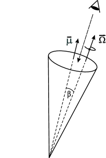
Figure 1: $\Omega$ is pulsar spin-axis,$\ \mu$ -axis of magnetic-momentum ($\beta\ll 1^{\circ}$)

It is well known that the distribution function of relativistic particles is one dimensional at the pulsar surface, because any transverse momenta ($p_{\perp}$) of relativistic electrons are lost during a very short time($\leq 10^{-20}$s) via synchrotron emission in very strong $B\sim 10^{11}$G magnetic fields. The distribution function is shown in Fig. 2 (Arons (1981)). For typical pulsars the plasma consists of the following components: the bulk of plasma with an average Lorentz-factor $\gamma_{p}\simeq 10$; a tail on the distribution function with $\gamma_{t}\simeq 10^{4}$ and the primary beam with $\gamma_{b}\simeq 10^{6}$. Though, plasma with an anisotropic distribution function becomes unstable that can lead to a wave excitation in the pulsar magnetosphere. The main mechanism of wave generation in plasmas of the pulsar magnetosphere is the cyclotron instability. The process can be conveniently described in cylindrical coordinates (see Fig. 3). The cyclotron resonance condition can be written in the form (Kazbegi, Machabeli & Melikidze (1991)):

$$\omega-k_{\varphi}V_{\varphi}-k_{x}u_{x}+\frac{\omega_{B}}{\gamma_{r}}=0,$$ (1)

where $V_{\varphi}\approx c(1-\frac{u_{x}^{2}}{c^{2}}-\frac{1}{2\gamma_{r}^{2}})$, $k_{\varphi}^{2}+k_{\perp}^{2}=k^{2}$, $k_{\perp}^{2}=k_{x}^{2}+k_{r}^{2}$, $\gamma_{r}$ is the Lorentz-factor for the resonant particles, $u_{x}$ is the drift velocity of the particles due to curvature of the field lines:

$$u_{x}=\frac{cV_{\varphi}\gamma_{r}}{\rho\omega_{B}},$$ (2)

where $\rho$ is the radius of curvature of the field lines and $\omega_{B}=eB/mc$ is the cyclotron frequency. The resonant condition for transverse (t) waves with the spectrum:

$$\omega_{t}=kc(1-\delta),$$ (3)

where

$$\delta=\frac{\omega_{p}^{2}}{4\omega_{B}^{2}\gamma_{p}^{3}},$$ (4)

takes the form:

$$\frac{1}{2\gamma_{r}}+\frac{\left(k_{\perp}/k_{\varphi}-u_{x}/c\right)^{2}}{2}+\frac{1}{2}\frac{k_{r}^{2}}{k_{\varphi}^{2}}-\delta=-\frac{\omega_{B}}{\gamma_{r}k_{\varphi}c}.$$ (5)

This equation describes the wave excitation process by the anomalous Doppler effect. During the quasi-linear stage of the instability a diffusion of particles arises not only along but also across the magnetic field lines. Therefore, plasma particles acquire transverse momenta (see Eq.12) and as a result the synchrotron mechanism is switched on.

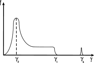
Figure 2: Distribution function of a one-dimensional plasma in the pulsar magnetosphere. Left corresponds to secondary particles, right to the primary beam.

The kinetic equation for the distribution function of the resonant particles can be written in the form (Machabeli & Usov (1979), Machabeli et al. (2002)):

$$\frac{\partial\textit{f}}{\partial t}+\frac{\partial}{\partial p_{\parallel}}\left[\left(G_{\parallel}+F_{\parallel}+Q_{\parallel}\right)\textit{f }\right]+\frac{1}{p_{\parallel}\psi}\frac{\partial}{\partial\psi}\left[\psi\left(G_{\perp}+F_{\perp}\right)\textit{f }\right]=$$

$$=\frac{1}{\psi}\frac{\partial}{\partial\psi}[\psi\left(D_{\perp,\perp}\frac{\partial}{\partial\psi}+D_{\perp,\parallel}\frac{\partial}{\partial p_{\parallel}}\right)\textit{f }\left(p_{\parallel},\psi\right)+$$

$$+\frac{\partial}{\partial p_{\parallel}}\left(D_{\parallel,\perp}\frac{\partial}{\partial\psi}+D_{\parallel,\parallel}\frac{\partial}{\partial p_{\parallel}}\right)\textit{f }\left(p_{\parallel},\psi\right)],$$ (6)

where $G$ is the force responsible for conservation of the adiabatic invariant $p_{\perp}^{2}/B(r)=$const, $F$- is the radiation deceleration force produced by synchrotron emission and $Q_{\parallel}$ is the reaction force of the curvature radiation. They can be written in the form:

$$G_{\perp}=-\frac{mc^{2}}{\rho}\gamma_{r}\psi,\qquad\qquad G_{\parallel}=\frac{mc^{2}}{\rho}\gamma_{r}\psi^{2},$$ (7)

$$F_{\perp}=-\alpha_{s}\psi\left(1+\gamma_{r}^{2}\psi^{2}\right),\qquad F_{\parallel}=-\alpha_{s}\gamma_{r}^{2}\psi^{2},$$ (8)

$$Q_{\parallel}=-\alpha_{c}\gamma_{r}^{4},$$ (9)

where $\alpha_{s}=2e^{2}\omega_{B}^{2}/3c^{2}$ and $\alpha_{c}=2e^{2}/3\rho^{2}$. For the $\textit{f}_{\parallel}$ the Eq. (6) will take the form:

$$\frac{\partial\textit{f}_{\parallel}}{\partial t}=\frac{\partial}{\partial p_{\parallel}}\left({\left[\alpha_{s}\psi_{0}^{2}\left(\frac{p_{\parallel}}{mc}\right)^{2}+\alpha_{c}\left(\frac{p_{\parallel}}{mc}\right)^{4}-2\pi^{2}\psi_{0}\frac{mc}{p_{\parallel}}r_{e}|E_{k}|^{2}\right]\textit{f}_{\parallel}}\right),$$ (10)

where $r_{e}=e^{2}/mc^{2}$, $\psi_{0}$ is the mean value of the pitch angle and $|E_{k}|^{2}$ is the density of electric energy in the waves.

The resultant spectrum of synchrotron emission is defined by the shape of distribution function of the resonant particles, which in turn is the solution of Eq. (10). To define the total flux emitted by the resonant particles we use the power of a single electron multiplied by the distribution function of emitting electrons and integrate the derived expression over the energy distribution (see Ginzburg (1981)).

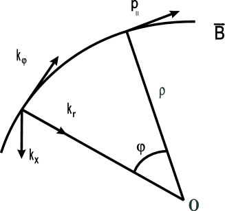
Figure 3: Coordinate system ($\rho$ is a local radius of curvature)

3 X-ray spectrum

We suppose that the measured X-ray spectrum is the result of synchrotron emission of primary beam electrons. Let us assume that before the cyclotron instability arises, the energy distribution in the beam has a shape:

$$\textit{f}_{b_{0}}=\frac{n_{b}}{\sqrt{\pi}\gamma_{T}}\textrm{ exp}\left[-\frac{\left(\gamma-\gamma_{b}\right)^{2}}{\gamma_{T}^{2}}\right],$$ (11)

where $\gamma_{b}\simeq 10^{6}$, $\gamma_{T}\simeq 10$ - is the half width of the distribution function and $n_{b}=B/Pce$ is the density of primary beam electrons, equal to the Goldreich-Julian density (Goldreich & Julian (1969)).

The wave excitation leads to a redistribution process of the particles via the quasi-linear diffusion. Let us compare relative values of all the three terms in the right-hand side of Eq. (10). Here we consider that $\gamma_{b}\psi_{0}\gg 1$ (the validity of this assumption will be estimated after obtaining the expression for $\psi_{0}$ ). In this case the equation for the diffusion across the magnetic field has the form (Malov & Machabeli 2002):

$$\frac{\partial\textit{f }_{b_{0}}}{\partial t}+\frac{1}{mc\gamma_{r}^{2}\psi}\frac{\partial}{\partial\psi}\left(\psi F_{\perp}\textit{f }_{b_{0}}\right)+\frac{1}{mc}\frac{\partial}{\partial\gamma_{b}}\left(F_{\parallel}\textit{f }_{b_{0}}\right)=$$

$$=\frac{1}{m^{2}c^{2}\gamma_{r}^{2}\psi}\frac{\partial}{\partial\psi}\left(\psi D_{\perp\perp}\frac{\partial\textit{f }_{b_{0}}}{\partial\psi}\right),$$ (12)

where

$$D_{\perp\perp}\approx\frac{\pi^{2}e^{2}}{m^{2}c^{3}}\frac{\delta}{\gamma_{b}^{2}}|E_{k}|^{2},$$ (13)

$$|E_{k}|^{2}=\frac{1}{2}\frac{mc^{2}n_{b}\gamma_{b}c}{\omega}.$$ (14)

The transversal quasi-linear diffusion increases the pitch-angle, whereas forces $\overrightarrow{G}$ and $\overrightarrow{F}$ resist this process, leading to the stationary state ($\partial\textit{f}/\partial t=0$). Then Eq. (12) gives the mean value of the angle $\psi$:

$$\psi_{0}=\frac{0.04\gamma_{b}^{3/4}}{BP^{3/4}\gamma_{p}\gamma_{r}^{1/2}}.$$ (15)

As a result of appearance of the pitch-angles the synchrotron emission is generated.

Using Eq. (15) we get:

$$\frac{\alpha_{c}\gamma_{r}^{4}}{\alpha_{s}\psi_{0}^{2}\gamma_{r}^{2}}\approx 10^{-10}\frac{\gamma_{r}^{3}\gamma_{p}^{2}}{\gamma_{b}^{3/2}P^{1/2}},$$ (16)

where P is the pulsar rotation period. We suppose that the period of RXJ1856 is $P\sim 1$s (this is a typical period for the pulsar with the age$\sim 10^{6}$yr). Using the parameter values indicated above, we will take that the quantity (16) is of order of 10.

Now let us compare the second and the third terms in the right-hand side of Eq. (10):

$$\frac{2\pi^{2}r_{e}\psi_{0}|E_{k}|^{2}/\gamma_{r}}{\alpha_{c}\gamma_{r}^{4}}\approx 10^{14}\frac{\gamma_{b}^{11/4}}{B^{2}P^{3/4}\gamma_{p}^{5}\gamma_{r}^{9/2}}.$$ (17)

We consider that the magnetic field is dipolar. Let us assume that for the primary-beam electrons the resonance condition is fulfilled at the distance $r\simeq 10^{9}$cm then for the magnetic field at the same distance, we will have $B\sim 10^{2}$G. For the parameter values pointed above, it turns out that, the third term of the Eq.(10) is by six orders of magnitude less than the second one. Then one gets:

$$\frac{\partial\textit{f}_{\parallel}}{\partial t}=\frac{1}{mc}\frac{\partial}{\partial\gamma_{b}}\left(\alpha_{c}\gamma_{b}^{4}\textit{f}_{\parallel}\right).$$ (18)

For $\gamma_{b}\psi\ll 10^{10}$, a magnetic field inhomogeneity does not affect the process of wave excitation. The equation which describes the cyclotron noise level, in this case has the form:

$$\frac{\partial|E_{k}|^{2}}{\partial t}=2\Gamma|E_{k}|^{2}\textit{f}_{\parallel},$$ (19)

where $\Gamma$ - is the growth rate of instability.

$$\Gamma=\pi\frac{\omega_{p_{res}}^{2}}{\omega_{0}\gamma_{T}}\qquad\textrm{if}\qquad\delta\gg\frac{1}{2}\frac{u_{x}^{2}}{c^{2}}$$ (20)

and

$$\Gamma=\pi\frac{\omega_{p_{res}}^{2}}{2\omega_{0}\gamma_{T}}\frac{u_{x}^{2}}{\delta c^{2}}\qquad\textrm{if}\qquad\delta\ll\frac{1}{2}\frac{u_{x}^{2}}{c^{2}},$$ (21)

where the resonant frequency is defined as (Kazbegi, Machabeli & Melikidze (1991))

$$\omega_{0}\approx\frac{\omega_{B}}{\delta\gamma_{r}}.$$ (22)

In this case we can use Eq. (21) for the growth rate and after substituting Eq. (19) in (18), we will take:

$$\frac{\partial}{\partial t}\left(\textit{f}_{\parallel}-\frac{\alpha_{c}}{m}\frac{\omega_{B}\gamma_{T}c}{\omega_{p_{res}}^{2}u^{2}}\frac{\partial}{\partial\gamma_{b}}\gamma_{b}^{3}\ln|E_{k}|^{2}\right)=0.$$ (23)

From this equation it is easy to find the distribution function:

$$\textit{f}_{\parallel_{b}}=\textit{f}_{\parallel_{b}0}+C\gamma_{b}^{2}.$$ (24)

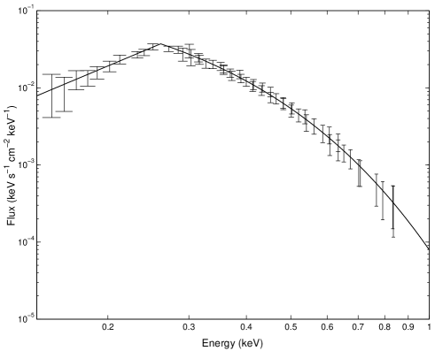
Figure 4: The Chandra LETG X-ray spectrum of RX J1856.5-3754 fitted with the model.

We suppose that the right slope of the measured X-ray spectrum is the result of synchrotron emission of the primary-beam electrons, with the distribution function (24), see Fig. 4.

In Malov & Machabeli (2002) it has been shown that it is possible to form the stationary distribution. If we assume $\partial\textit{f}_{\parallel}/\partial t=0$, then from Eq. (18) one finds:

$$\textit{f}_{\parallel_{b}}\propto\gamma_{b}^{-4}.$$ (25)

We consider that after the quasi-linear evolution stage of the instability, by achieving the stationary state, the radiation density is significant and the self-absorption effects begin to play the main role. Synchrotron self-absorption, redistributes the emission spectrum and in the domain of relatively low frequencies, we have (Zhelezniakov (1977)):

$$I(\nu)\propto\nu^{5/2}.$$ (26)

This emission corresponds to energy interval (0.15-0.26 keV) of the measured X-ray spectrum (see Fig. 4).

The frequency of the maximum of measured X-ray spectrum corresponds to the intersection point of theoretical curves, fitted with the observed data ($\nu\simeq 6\cdot 10^{16}$Hz). On the other hand, the frequency of the maximum of synchrotron spectrum of a single electron is (Pacholczyk et al. (1970)):

$$\nu_{m}\simeq 0.07\frac{eB}{mc}sin\psi\gamma_{b}^{2}.$$ (27)

Using Eq. (15) for $\psi\ll 1$, we find that the frequency of maximum of the spectrum turns out to be not dependent on magnetic field. Consequently, we can estimate from Eq. (27) the rotation period of RXJ1856. Estimations show that $P\sim 1$s, i.e. the primitive conjecture proves to be true. The same can be found about two other assumptions done at the beginning of our computations, since $\psi_{0b}\sim 10^{-3}\ll 1$ and $\gamma_{b}\psi_{0b}\sim 10^{3}$.

4 Optical spectrum

Now let us consider the observed optical emission of RXJ1856. We suppose that this emission is related with electrons of a tail, with an average Lorentz-factor $\gamma_{t}\simeq 10^{4}$. Let us assume that the initial distribution of particles of the tail has the following form (see Fig. 2):

$$\textit{f}_{t_{0}}\propto\gamma^{-4}.$$ (28)

As in the previous case, one needs to estimate the contribution of different terms in the right-hand side of Eq. (10). We suppose that the condition $\gamma_{t}\psi_{0}\gg 1$ is fulfilled and we can use Eq. (15) for the mean value of angle $\psi$ in this case too. For values of parameters indicated above we take that, the first term exceeds the second one by five orders of magnitude. Now let us compare the first and the third terms:

$$\frac{2\pi^{2}r_{e}\psi_{0}|E_{k}|^{2}/\gamma_{t}}{\alpha_{s}\psi_{0}^{2}\gamma_{r}^{2}}\approx 1.3\cdot 10^{4}\frac{\gamma_{b}^{5/4}}{B^{2}P^{5/4}\gamma_{p}^{3}\gamma_{t}^{3/2}}.$$ (29)

We suppose that for the electrons of the tail, the cyclotron resonance condition is fulfilled at the distance $r\simeq 3\cdot 10^{9}$cm and for the value of the magnetic field we take $B\sim 1$G. Finally, after substituting values in Eq. (29) we take that the third term is less than the first one by an order of magnitude.

Consequently, instead of Eq. (10), we will have:

$$\frac{\partial\textit{f}_{\parallel}}{\partial t}+\frac{2\pi^{2}\psi_{0}r_{e}}{mc}\frac{\partial}{\partial\gamma}\left(\frac{|E_{k}|^{2}}{\gamma}\textit{f}_{\parallel}\right)=0.$$ (30)

In this case we can use Eq. (20) for the growth rate of instability and from Eqs. (19) and (30) one gets:

$$\frac{\partial}{\partial t}\left(\textit{f}_{\parallel}+\frac{\pi^{2}e^{2}\omega_{B}\gamma_{T}}{m^{2}c^{3}\delta\omega_{p_{t}}^{2}}\psi_{0}\frac{\partial}{\partial\gamma}\frac{|E_{k}|^{2}}{\gamma^{2}}\right)=0.$$ (31)

From this equation we can find the expression for $|E_{k}|^{2}$ at the final moment of the quasi-linear stage. If we take into account that the density of the particles behaves as $1/r^{3}$ ($r$ is the distance from the pulsar), one can neglect $\textit{f}_{\parallel_{t}}$ in comparison with $\textit{f}_{\parallel_{t}0}$ and from Eq. (31) one finds:

$$|E_{k}|^{2}\approx\frac{m^{2}c^{3}\delta\omega_{p_{t}}^{2}}{2\pi^{2}e^{2}\omega_{B}\gamma_{T}\psi_{0}\gamma}.$$ (32)

After achieving the stationary mode, the distribution function of particles of the tail can be found from Eq. (30) if one sets $\partial\textit{f}_{\parallel}/\partial t=0$, then we will take:

$$\textit{f}_{\parallel}\propto|E_{k}|^{-2}\gamma.$$ (33)

Using Eq. (32) for the $|E_{k}|^{-2}$ we find:

$$\textit{f}_{\parallel_{t}}\propto\gamma^{2}.$$ (34)

The resultant theoretical spectrum is well matched with the measured one. For parameters used above, we find that indeed $\gamma_{t}\psi_{0t}\sim 10^{3}\gg 1$ ($\psi_{0t}\simeq 3\cdot 10^{-1}$).

The frequency of the maximum in synchrotron emission of a single electron is defined by Eq. (27). For the parameter values used above, we will take $\nu_{m}(Optic)\simeq 2\cdot 10^{14}$Hz. This quantity comes in the domain that corresponds the observed optical data.

5 The effectiveness of the cyclotron mechanism

Now let us estimate the frequencies of original waves, excited during the cyclotron resonance. Using the same parameters, one can see from Eq. (22) that the frequencies corresponding to the beam and tail components are $\nu\approx 3\cdot 10^{9}$Hz and $\nu\approx 5\cdot 10^{8}$Hz respectively, i.e. during the cyclotron resonance in both cases the radio waves are excited. Though this waves are generated earlier than X-ray and optical emission and therefore the radio emission might pass by line of sight. In this case the radio emission will not get to observer. That is one of possible explanations why the radio emission is not detected from this object.

For effective generation of waves it is essential that time, during which the particles give energy to waves should be more than $1/\Gamma$. Generated radio waves propagate practically in straight lines, whereas the field line of the dipole magnetic field deviates from its initial direction and the angle $\theta=k_{\parallel}/k_{\varphi}$ grows ($\theta$ is the angle between the wave line and the line of dipole magnetic field). On the other hand, the resonance condition (5) imposes limitations on $\theta\approx\textrm{max}\{\sqrt{\delta},\frac{u_{x}}{c}\}$ (Kazbegi, Machabeli & Melikidze (1991)), i.e. particles can resonate with the waves propagating in a limited range of angles. Obviously the Eq. (5) will be fulfilled until then (Lyutikov, Blandford & Machabeli (1999)):

$$\frac{c}{\Gamma}\lesssim\theta\rho,$$ (35)

where $c\Gamma^{-1}$ is the growth length and $\theta\rho$ is the length of the wave-particle interaction. For the beam particles from Eq. (35) it follows that $\rho\gtrsim 3\cdot 10^{9}$cm. As the cyclotron instability arises at distances $r\simeq 10^{9}$cm for the beam electrons, this result means that time of wave interaction with the resonant particles is quite enough for particles to acquire the pith-angles $\psi_{0}$ (Eq. 15), which automatically leads to the generation of synchrotron emission.

The total energy available for the conversion into pulsar emission is of the order of the energy of primary beam particles flowing along the open filed lines of the pulsar magnetosphere:

$$\dot{E}\simeq n_{b_{0}}\pi R_{pc}^{2}\gamma_{b}mc^{3},$$ (36)

where $n_{b_{0}}$ is the Goldreich-Julian density at the pulsar surface and $R_{pc}$ is the radius of the polar cap. The estimations show $\dot{E}\simeq 5\cdot 10^{32}$erg/s, which is quite enough to explain the observed luminosity of RXJ1856.

6 Conclusions

1. In the present paper we assume that the emission of RXJ1856 is generated by the synchrotron mechanism. The main reason of wave generation in outer parts of the pulsar magnetosphere is the cyclotron instability. During the quasi-linear stage of the instability a diffusion of particles arises as along, also across the magnetic field. Plasma particles acquire pitch angles and begin to rotate along the Larmor orbits. Synchrotron emission is the result of the appearance of pitch angles.

2. The measured X-ray spectrum is the result of synchrotron emission of primary-beam electrons, generated at distances $r\simeq 10^{9}$cm, when the optical emission is related with secondary plasma particles, particularly the tail electrons. The optical spectrum is produced by synchrotron emission of the tail electrons, generated at distances $r\simeq 3\cdot 10^{9}$cm. The predictable characteristic frequencies $\nu_{m}(X-ray)\simeq 6\cdot 10^{16}$Hz and $\nu_{m}(Optic)\simeq 2\cdot 10^{14}$Hz come in the same domains as the measured spectra.

3. The observed optical emission reveals an intensity six times larger than the X-ray one. The X-ray emission is generated earlier in contrast to optical emission. Thus, an observer may receive only part of the radiation emitted in the X-ray domain. We suggest that this must be the reason of lower intensity of the X-ray spectrum.

4. In view of the fact that the aligned rotator model is used, the radio emission covers a large distance in the pulsar magnetosphere. So there is a high probability for it to come in the cyclotron damping range $\omega-k_{\varphi}V_{\varphi}-k_{x}u_{x}-\frac{\omega_{B}}{\gamma_{r}}=0$. In this case the radio emission will not reach an observer. Another explanation of the lack of radio emission from this object is that the X-ray and optical emission, resulted from the quasi-linear diffusion, occur in a region further away from that of the radio emission and it miss our line of sight. Nevertheless the detection of radio emission from RXJ1856 would be strong argument to our model.

5. We give estimations of effectiveness of the cyclotron mechanism, which in this case means the fulfillment of the following condition $\rho\gtrsim 3\cdot 10^{9}$cm. As the instability develops at distances $r\simeq 10^{9}$cm, then follows that the excited waves lie in the resonant region sufficiently long time, which is quite enough for particles to acquire perpendicular momentum and generate radiation.