Microscale swimming: The molecular dynamics approach

Abstract

The self-propelled motion of microscopic bodies immersed in a fluid medium is studied using molecular dynamics simulation. The advantage of the atomistic approach is that the detailed level of description allows complete freedom in specifying the swimmer design and its coupling with the surrounding fluid. A series of two-dimensional swimming bodies employing a variety of propulsion mechanisms – motivated by biological and microrobotic designs – is investigated, including the use of moving limbs, changing body shapes and fluid jets. The swimming efficiency and the nature of the induced, time-dependent flow fields are found to differ widely among body designs and propulsion mechanisms.

I Introduction

There is a growing demand – driven by nanotechnology – to understand and utilize nanoscale hydrodynamical phenomena, a consequence of which is the need to achieve a capability for detailed modeling of the underlying physical processes occurring at submicroscopic scales. There are numerous instances where nature itself provides examples of successful design at this level, a regime where behavior runs contrary to the familiar macroscopic world; emulating some of the multitude of biological architectures and mechanisms may, therefore, provide insight into the requirements for optimized engineering design.

Microrobotics has long captured the imagination Feynman (1960), with practical implementations only now becoming feasible. One category of microrobot with potential medical applications employs self-propelled swimming; however, long before such devices were envisaged, studies of the dynamics of microscopic life forms, and the theoretical analysis of hydrodynamics at appropriately low Reynolds numbers, $Re\approx 10^{-5}$, made it clear that the prevailing fluid environments were unlike those encountered in more familiar circumstances (where $Re\gg 1$) but rather resembled slow swimming in highly viscous treacle. This is known as Stokes (or creeping) flow, and responsibility for the counterintuitive behavior lies in the absence of inertia from the dynamics Happel and Brenner (1983). Microscopic creatures swim by employing mechanisms appropriate to these conditions, such as rotating flagella, beating cilia, body deformation, and longitudinal or transverse surface waves Purcell (1977); Childress (1981); Vogel (1994). While microscale robots may need to travel faster than their target biological organisms in the fluid medium, their motion relative to the fluid would still be at low $Re$.

Low-$Re$ flow is amenable to theoretical analysis because the limiting form of the Navier–Stokes equation is linear and time independent Happel and Brenner (1983); in this limit, the motion of self-propelled bodies can be studied using suitable approximations, perturbation methods and simple models, e.g., Shapere and Wilczek (1987); Ehlers et al. (1996); Stone and Samuel (1996); Becker et al. (2003); Avron et al. (2004); Najafi and Golestanian (2004); Avron et al. (2005); Felderhof (2006). Microscopic swimmers have also been synthesized experimentally Dreyfus et al. (2005). Swimming has been studied numerically, based on a continuum fluid (with grid discretization) and the immersed-boundary method for dealing with the interface between the fluid and an elastic body Cortez et al. (2004), and mesoscopically described fluids utilizing, e.g., the lattice-Boltzmann method, have also been used Earl et al. (2007).

The present study of microswimmers is based on molecular dynamics (MD) simulation Rapaport (2004), in which the fluid itself consists of discrete atoms that interact directly with the swimmer. The MD approach is flexible in regard to the level of structural detail that can be incorporated and, unlike other approaches, hydrodynamic correlations emerge naturally. A selection of self-propelled bodies that swim using a variety of mechanisms is investigated; a particularly important aspect of the results is a comparison of the efficiency of the alternative body designs and propulsion techniques.

The MD approach is motivated and justified by its success with other hydrodynamical problems, e.g., hexagonal flow patterns in Rayleigh–Bénard convection Rapaport (2006) and toroidal rolls in Taylor–Couette flow Hirshfeld and Rapaport (1998, 2000), the latter even in quantitative agreement with continuum theory. Although large driving forces and gradients are required to compensate for small size in order to exceed the instability threshold, MD demonstrates continuum-like behavior in fluid layers a mere 30 atomic diameters thick. Thus the scaling implicit in dynamic similarity extends down to the MD regime, although there is an eventual lower size limit Vergeles et al. (1995).

II Methodology

The swimmer is immersed in a two-dimensional (2D) fluid (where computation requirements are reduced substantially and flow visualization simplified compared to 3D) confined to a rectangular container. The body and limbs of the swimmer are constructed from soft-disk atoms. Each atom is placed at a particular location relative to a reference coordinate frame attached to the body; the locations are either fixed in the frame if they form the body, or follow predetermined periodic paths if they belong to a limb or other moving component of the propulsion mechanism. The atoms interact via a short-range, repulsive interaction, $U(r)=4\epsilon[(\sigma/r)^{12}-(\sigma/r)^{6}]$, with range $r<r_{c}=2^{1/6}\sigma$. The atom spacing in the swimmer is $1.1\sigma$, producing a rough boundary to oppose fluid slip; while a hindrance at higher $Re$ where drag reduction is important, skin drag is necessary for certain kinds of low-$Re$ propulsion. Swimmer mass is proportional to displaced fluid area (excluding limbs); while motion is not totally inertia free, it approaches this limit at low speeds. The container boundaries are made from fixed atoms, spaced to produce impenetrable, nonslip walls (periodic boundaries are unsuitable as they would allow bulk flow). Finally, there are the moving atoms of the fluid; fluid properties such as viscosity are intrinsic to the model and depend on the intermolecular forces, density, and temperature (in contrast to a continuum representation where viscosity is normally an assigned parameter).

Interactions among fluid atoms, as well as between fluid atoms and the swimmer components and walls are computed at each MD timestep; the total force acting on the swimmer (and torque, if needed) is evaluated from contributions of all fluid atoms within range $r_{c}$ of any of the swimmer atoms. Standard MD techniques Rapaport (2004) are used in the force computations (for larger systems the task can be parallelized), the equations of motion of the fluid atoms and swimmer center-of-mass (c.m.) are integrated using a leapfrog algorithm, and a thermostat is applied to prevent viscous heating.

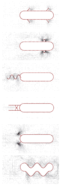
Figure 1: A selection of swimmer designs: biflaps, cigar, flagellum, jet, legs and snake; flow fields are shown.

A broad range of swimmer designs employing different propulsion modes are considered; they are described below, and several are shown in Fig. 1. Some designs aim to emulate biological life forms manifest at various size scales Childress (1981); Berg (1983); Vogel (1994), while others implement theoretical models (organisms that appear biologically infeasible might be realizable artificially). Most designs are based on a cylinder – where the term ‘cylinder’ refers to the 2D projection of a cigar (or spherocylinder) – with the same frontal area and body length to allow comparison of relative performance. Each swimmer executes closed periodic cycles in the appropriate internal-coordinate space; most cycles are irreversible, an essential requirement for propulsion in the Stokes regime Purcell (1977). Swimmer names are indicative of shape or propulsion mechanism.

Biflaps: two pairs of lateral flaps near the front and rear rotate from the forward direction through $90^{\circ}$ and retract. Cigar: two curved paddles emerge laterally near the front, slide along the body to near the rear and retract – multiple paddles would resemble a transverse wave Ehlers et al. (1996). Flagellum: a flexible rear-pointing tail along which a transverse, two-cycle sinusoidal wave propagates – the 2D equivalent of a rotating helix. Flaps: a single pair of lateral flaps near the front. Jet: an open cavity at the rear into which paddles emerge from the inner walls and slide rearwards acting as a piston to expel the fluid, the paddles retract and there is a recovery period for refilling the cavity – an approximation of squid propulsion. Legs: a pair of flaps emerges laterally at the rear, rotates backwards through $90^{\circ}$ and retracts. Slime: a circular body that extends a thin hollow rod (to a distance equal to the initial radius) at the end of which a new circular body grows (at constant areal rate) while the initial body contracts (total area is fixed), and the rod finally retracts into the new body – a related system is treated theoretically in Avron et al. (2005).

Snake: based on a cylinder whose central axis is displaced laterally to follow a two-cycle traveling sine wave. Tail: a rigid, rear-pointing oar oscillates sinusoidally over a $36^{\circ}$ range; this mechanism, unlike the others, is time-reversible, and under Stokes conditions swimming is impossible Purcell (1977). Track: the atoms forming the sidewalls slide along the body, emerging from behind the front cap and disappearing into the rear, and propulsion is due to the skin drag of the rough boundary; this is an approximation of a membrane extruded at the front and absorbed at the rear, or the longitudinal surface waves of cilia Childress (1981); Vogel (1994). Trilinear: three linked circular bodies, joined linearly by rods whose lengths vary with time in an irreversible cycle Najafi and Golestanian (2004). Tube: hollow cylinder open to the fluid at both ends with the same frontal area as the other cylindrical bodies; two paddles emerge inwards, slide to the rear expelling fluid, and retract – a ‘peristaltic’ mechanism.

The swimmer cylinder length is $L_{b}=75$; reduced MD units are used, where the length unit is $\sigma=$ 0.34 nm, so that the actual length is 26 nm. Although this is several orders of magnitude less than even the smallest of organisms, the MD flow studies cited earlier indicate that this should not adversely affect the results. Other swimmer dimensions are proportional to $L_{b}$; the radius is $R_{b}=L_{b}/6$ (also the maximum radius of slime), so the total body length is $4L_{b}/3=100$, flap and leg lengths are $L_{b}/6$, tail oar length $L_{b}/3$, snake amplitude $L_{b}/10$; these and other design elements represent reasonable (though arbitrary) choices. Careful design is required to prevent fluid atoms becoming trapped in a corner by a moving limb; since only the time-dependent limb position is specified, this would cause numerical instability. Swimmer components whose size varies (such as the growing flap) accomplish this by altering the atom overlap. The swimmer c.m. is constrained to move in a straight line and body rotation is not allowed, otherwise travel direction would be subject to random change (Brownian motion), complicating the analysis.

A large container is required to help dissipate induced flows and ensure the swimmer remains far from the walls; container size is $835\times 338$, and for fluid density 0.7 the total number of atoms is approximately 190 000. Runs begin with the swimmer at rest (except for towed bodies), positioned several body lengths from the rear wall; the fluid atoms are assigned random velocities with a rms value of unity, and arranged on a triangular lattice (outside the swimmer). Run length is 610 000 timesteps (the first 10 000 are excluded from analysis) of size 0.005 (MD time unit $\sqrt{m\sigma^{2}/\epsilon}=$ 2.2 ps, where $m$ is the atom mass).

The rate of change of the internal swimmer state is governed by the drive speed $v_{d}$; this corresponds to the (fixed or highest) speed of a sliding component or the tip of a rotating limb in the swimmer reference frame. The value of $v_{d}$ determines the cycle period and, after allowing for interaction with the fluid, the average swim speed and power dissipation; $v_{d}$ must be relatively small to minimize density fluctuations in the (compressible) fluid and local shear rates, but sufficiently large that runs are of reasonable duration.

Two externally towed bodies are included for comparison, moving at fixed speed irrespective of the fluctuating fluid forces. Cylinder: the basic body design used for most swimmers. Disk: a circular body with radius $R_{b}$, but without the extra skin drag of the cylinder body.

III Results

Examples of the structured, time-varying flows that develop (for $v_{d}=0.6$) appear in Fig. 1 (fluid atoms are not shown); swim direction is to the right. The spatially coarse-grained flow is evaluated over a rectangular grid attached to the swimmer, with velocities measured in a stationary frame; the swim cycle is divided into 16 phase segments and each is averaged separately over the run. Only a single segment is shown for each swimmer, but the phase chosen is where the flow best reflects the nature of the propulsion mechanism. Only the fluid region close to the swimmer is included to ensure adequate resolution; furthermore, the longest arrow for each swimmer corresponds to the highest flow speed anywhere in its cycle, and may not appear in the selected phase.

Figure 2: Cycle-averaged power as a function of swim speed for different swimmers and drive speeds (MD units); separate graphs (with different scales) show (a) the most efficient of the swimmers and the towed bodies, and (b) swimmers of moderate efficiency.

Fig. 2 shows the average power $\langle P\rangle$ required to overcome fluid resistance and maintain a mean swim speed $\langle v_{s}\rangle$ for several of the swimmers; the points on each performance curve are for different $v_{d}$ or towing speed (in most cases 0.1, 0.2, 0.4 and 0.6, but reduced by factors of 2, 4 and 10 for slime, track and the towed bodies, respectively). $P$ is the total work per unit time performed by swimmer atoms (both in the body and the propulsion mechanism) against the forces exerted by fluid atoms within range $r_{c}$. $\langle v_{s}\rangle$ is small relative to the fluid thermal velocity. The results are consistent with $\langle v_{s}\rangle$ being proportional to $v_{d}$, a consequence of the linearity of the flow problem.

Higher efficiency implies reduced power for a given swim speed; the ratio $\langle P\rangle/\langle v_{s}\rangle$ provides a measure of performance – the lower the better. Efficiency differs considerably among swimmer designs, and for a given $v_{d}$, some are faster (possibly utilizing more power) than others. Relative to the towed reference cylinder (which provides a measure of the useful work done), track achieves a comparatively high efficiency of about 17%, as well as an effective coupling of the body wall to the fluid since $\langle v_{s}\rangle\approx v_{d}/3$, while for cigar efficiency is 2%, and only 1% for tube; such results lie in the expected range Stone and Samuel (1996). The remaining swimmers either have lower efficiency or move even more slowly (briefly, for $v_{d}=0.6$, flaps, flagellum and tail have $\langle v_{s}\rangle=0.04\pm 0.01$ at $\langle P\rangle\approx 5$, jet has $\langle v_{s}\rangle=0.04$ at $\langle P\rangle=11$, while trilinear is even slower and less efficient). It should be noted that these comparisons are applicable to the specific swimmers described here; the designs have not been optimized for maximum performance.

Establishing the relevance of the MD approach requires an estimate of $Re$. For the midrange speed $\langle v_{s}\rangle=0.04$, and a measured kinematic viscosity $\nu=2.1$ (from an MD analysis of 2D pipe flow – not shown), $Re=2R_{b}\langle v_{s}\rangle/\nu\approx 0.5$, a value where inertial effects can be disregarded Batchelor (1967). Since the limb speeds are higher, inertial effects might be present at smaller length scales (explaining the motion of tail). The towed-body data can be fit to $\langle P\rangle=Cv_{s}^{2}$, the functional form of simple Stokes drag, with $C_{disk}=11.5$ and $C_{cylinder}=18$ ($<0.003$ deviation); the latter is larger due to skin friction of the elongated body, in addition to pressure drag common to both.

Figure 3: Dependence of (a) instantaneous power and (b) swim speed on phase angle.

Fig. 3 shows the dependence of the instantaneous speed and power, $v_{s}$ and $P$, on phase angle, for $v_{d}=0.4$; the results are averaged over the corresponding phases of all cycles in the run (15–35, depending on swimmer). Peak values can be much larger than average, a significant design issue, while the low $v_{s}$ during the phase when propulsion is absent shows that inertial effects are small ($P<0$ corresponds to deceleration). Each swimmer has its own characteristic behavior reflecting the mode of propulsion. In the examples shown, high power is needed by biflaps early in the cycle to build up speed that then drops steadily, tube has an even more sharply peaked early speed, for legs the increase in power and speed occurs as the flaps approach the rear, while the values are almost constant during the sliding portion of the cigar cycle.

In conclusion, the capabilities of a variety of swimmer designs have been analyzed using an MD approach built on particle-based swimmers and fluid. The results demonstrate that MD is a viable tool for modeling swimming on the microscopic scale and, more specifically, that swimming efficiency varies widely among swimmer body designs and propulsion mechanisms. Since MD is limited only by computational resources, it has the potential to play an important role in the study of microrobotic swimmers, a field holding enormous industrial and therapeutic promise.

References

- Feynman (1960) R. P. Feynman, Eng. Sci. 23, 22 (1960).
- Happel and Brenner (1983) J. Happel and H. Brenner, Low Reynolds Number Hydrodynamics (Martinus Nijhoff, The Hague, 1983).
- Purcell (1977) E. M. Purcell, Am. J. Physics 45, 3 (1977).
- Childress (1981) S. Childress, Mechanics of Swimming and Flying (Cambridge University Press, Cambridge, 1981).
- Vogel (1994) S. Vogel, Life in Moving Fluids: The Physical Biology of Flow (Princeton University Press, Princeton, 1994), 2nd ed.
- Shapere and Wilczek (1987) A. Shapere and F. Wilczek, Phys. Rev. Lett. 58, 2051 (1987).
- Ehlers et al. (1996) K. M. Ehlers, A. D. T. Samuel, H. C. Berg, and R. Montgomery, Proc. Natl. Acad. Sci. USA 93, 8340 (1996).
- Stone and Samuel (1996) H. A. Stone and A. D. T. Samuel, Phys. Rev. Lett. 77, 4102 (1996).
- Becker et al. (2003) L. E. Becker, S. A. Koehler, and H. A. Stone, J. Fluid Mech. 490, 15 (2003).
- Avron et al. (2004) J. E. Avron, O. Gat, and O. Kenneth, Phys. Rev. Lett. 93, 186001 (2004).
- Najafi and Golestanian (2004) A. Najafi and R. Golestanian, Phys. Rev. E 69, 062901 (2004).
- Avron et al. (2005) J. E. Avron, O. Kenneth, and D. H. Oaknin, New J. Phys. 7, 234 (2005).
- Felderhof (2006) B. U. Felderhof, Phys. Fluids 18, 063101 (2006).
- Dreyfus et al. (2005) R. Dreyfus, J. Baudry, M. L. Roper, M. Fermigier, H. A. Stone, and J. Bibette, Nature 437, 862 (2005).
- Cortez et al. (2004) R. Cortez, L. Fauci, N. Cowen, and R. Dillon, Computing in Sci. and Eng. 6, 38 (2004).
- Earl et al. (2007) D. J. Earl, C. M. Pooley, J. F. Ryder, I. Bredberg, and J. M. Yeomans, J. Chem. Phys. 126, 064703 (2007).
- Rapaport (2004) D. C. Rapaport, The Art of Molecular Dynamics Simulation (Cambridge University Press, Cambridge, 2004), 2nd ed.
- Rapaport (2006) D. C. Rapaport, Phys. Rev. E 73, 025301(R) (2006).
- Hirshfeld and Rapaport (1998) D. Hirshfeld and D. C. Rapaport, Phys. Rev. Lett. 80, 5337 (1998).
- Hirshfeld and Rapaport (2000) D. Hirshfeld and D. C. Rapaport, Phys. Rev. E 61, R21 (2000).
- Vergeles et al. (1995) M. Vergeles, P. Keblinski, J. Koplik, and J. R. Banavar, Phys. Rev. Lett. 75, 232 (1995).
- Berg (1983) H. Berg, Random Walks in Biology (Princeton University Press, Princeton, 1983).
- Batchelor (1967) G. K. Batchelor, An Introduction to Fluid Dynamics (Cambridge University Press, Cambridge, 1967).