T. Nishimichi et al. Characteristic Scales of Baryon Acoustic Oscillations from Perturbation Theory \Received2007/05/02\Accepted2007/08/??
cosmology: large-scale structure of universe — theory — methods: statistical
Characteristic Scales of Baryon Acoustic Oscillations from Perturbation Theory: Non-linearity and Redshift-Space Distortion Effects
Abstract
An acoustic oscillation of the primeval photon-baryon fluid around the decoupling time imprints a characteristic scale in the galaxy distribution today, known as the baryon acoustic oscillation (BAO) scale. Several on-going and/or future galaxy surveys aim at detecting and precisely determining the BAO scale so as to trace the expansion history of the universe. We consider nonlinear and redshift-space distortion effects on the shifts of the BAO scale in -space using perturbation theory. The resulting shifts are indeed sensitive to different choices of the definition of the BAO scale, which needs to be kept in mind in the data analysis. We present a toy model to explain the physical behavior of the shifts. We find that the BAO scale defined as in Percival et al. (2007) indeed shows very small shifts () relative to the prediction in linear theory in real space. The shifts can be predicted accurately for scales where the perturbation theory is reliable.
1 Introduction
The baryon acoustic oscillation (BAO) is an oscillation of photon-baryon fluid imprinted in the matter spectrum as a characteristic signature. Recently it was detected in the SDSS and 2dFGRS galaxy distribution (e.g., [Eisenstein et al. (2005), Hütsi (2006), Tegmark et al. (2006), Padmanabhan et al. (2006), Percival et al. (2007), Cole et al. (2005)]), while its counterpart in the cosmic microwave background (CMB) has already played an important role in precision cosmology (Spergel et al., 2007). Currently, using the BAO scale as a standard ruler is regarded as one of the most promising tools to trace the cosmic expansion history. This characteristic scale basically corresponds to the sound horizon at recombination (e.g., Eisenstein et al. (2005), and see also Appendix A):
| (1) | |||||
| (2) | |||||
| (3) |
where is the sound speed at redshift , and is the redshift at recombination (). In the second equality, is the horizon scale at the matter-radiation equality epoch, , and are the ratio of the baryon to photon momentum densities at and . Finally the last equality is an approximate fit where and are the density parameters of matter and baryon, and is the current Hubble constant in units of 100km s-1Mpc-1.
The BAO length scale itself can be computed accurately and is indeed insensitive to the presence of dark energy that affects the expansion of the universe at relatively low redshifts. Precisely for these reasons, it is a useful standard ruler of the universe. In particular, it is supposed to be a good tracer of , where and are the pressure and the density of dark energy (e.g., Blake & Glazebrook (2003); Seo & Eisenstein (2003)). Also it can potentially be used to falsify the possibility of alternative law of gravity which might explain the acceleration of the cosmic expansion (Shirata et al., 2005; Yamamoto et al., 2006).
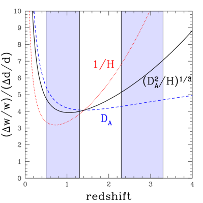
Consider a sample of galaxies with measured redshifts, the observed BAO scale provides estimates of the angular diameter distance and the inverse of the Hubble parameter , which correspond to the scales perpendicular and parallel to the line-of-sight direction, respectively. They in turn can be translated into the estimate of . Figure 1 shows how the fractional errors of three important scales, the angular diameter distance , the inverse of Hubble parameter and their average over three dimensions propagate to that of . The cosmological parameters assumed are the third year WMAP results (Spergel et al. (2007), see section 3 for details). The two shaded regions show the approximate targeted redshift ranges of a future galaxy redshift survey, WFMOS (Wide-field Fiber-fed Multi-Object Spectrograph). Typically a ratio of and around ranges from 3 to 5, while the value depends slightly on a specific choice of cosmological parameters. Thus the % determination of requires the sub-percent accuracy/precision in determining the BAO scale, which is challenging from observational, and even theoretical, points of view.
Until recently it was often assumed that gravitational non-linearity and redshift-distortion effects do not shift the BAO scale, although they significantly affect the amplitude of the BAO. Some simulations (e.g., Meiksin, White & Peacock (1999); Seo & Eisenstein (2005); Springel et al. (2005); Angulo et al. (2005); Jeong & Komatsu (2006); Ma (2006); Eisenstein et al. (2006); Angulo et al. (2007)) and analytical works (e.g., Eisenstein, Seo & White (2006); Guzik, Bernstein & Smith (2007); Smith, Scoccimarro & Sheth 2007a; Smith, Scoccimarro & Sheth 2007b) have been done to study these effects on the power spectrum or two-point correlation function at the BAO scale. For a few percent accuracy on , more precise BAO predictions are required, which we consider in the present paper on the basis of the one-loop corrections from perturbation theory.
Very recently, several authors (Crocce & Scoccimarro 2006a; Crocce & Scoccimarro 2006b; McDonald (2007); Valageas (2007); Padmanabhan & Ray (2006); Matarrese & Pietroni 2007a; Matarrese & Pietroni 2007b; Crocce & Scoccimarro (2007)) attempt to take account of higher-order corrections. For the first time, we take account of the redshift-space distortion effects on the BAO scale applying the result of Scoccimarro (2004).
The outline of this paper is as follows; section 2 briefly summarizes the perturbation theory of density and velocity fields. The details of the numerical calculation are shown in section 3. The results are shown in section 4 with discussion and interpretation in section 5. Finally, section 6 is devoted to the conclusion of this paper.
2 Non-linear power spectrum in real and redshift spaces
Cosmological perturbation theory predicts the gravitational clustering of matter distribution by a systematic expansion of the cosmological density and velocity fields. It provides us an accurate prediction to the non-linear modification of matter power spectrum as long as the gravitational clustering is mildly non-linear (e.g., Juszkiewicz (1981); Vishniac (1983); Fry (1984); Goroff et al. (1986); Suto & Sasaki (1991); Makino, Sasaki & Suto (1992); Jain & Bertschinger (1994); Bernardeau (1994); Matsubara (1995); Scoccimarro et al. (1998); Chodorowski & Ciecielag (2002), and see Bernardeau et al. (2002) for a review). In this section, we briefly review the formalism to calculate the non-linear correction to the matter power spectrum. A model of redshift-space distortion is also presented, which will be used later to estimate the non-linearity of redshift-space power spectrum.
2.1 Perturbation theory
To deal with the gravitational clustering of the matter distribution, we adopt the hydrodynamic description and treat the dark matter and baryons as a pressureless dust fluid. According to Scoccimarro (2001), the evolution equations for the cosmic fluid can be written in a compact form by introducing the two-component vector:
| (4) |
where the subscript selects the density or velocity components, with and respectively being the Fourier transform of the density fluctuation and peculiar velocity divergence. The variable represents the time variable defined by , where is the linear growth factor normalized to unity at present. The quantity is the conformal expansion rate given by , where is the cosmic scale factor, and the quantity is the logarithmic derivative of the linear growth factor, .
Assuming the irrotational fluid flow, the evolution equations can then be written as
| (5) |
where the kernel is the vertex matrix which represents the non-linear interaction between different Fourier modes:
| (10) |
with being Dirac’s delta function. The matrix is given by
| (13) |
This expression is not exact in the non Einstein-de Sitter cases, but it still provides an accurate prescription.
The evolution equation given above is systematically solved by a perturbative expansion of two-component vector. Ignoring the decaying modes, one obtains
| (14) | |||||
| (15) |
where the quantity stands for the initial density fluctuation, which we assume is a Gaussian random variable. The Fourier kernel represents the mode coupling between different Fourier modes originating from the non-linear interactions. In Appendix B, the explicit expressions for are presented up to the third-order of perturbative expansion.
We are interested in the non-linear evolution of power spectrum, which are evaluated as the ensemble average of the quantity :
| (16) |
Note that we obtain the three different power spectra: from , from and , and from . Substituting the solutions (14) up to the third-order perturbations into the above, the next-to-leading order corrections are obtained, which can be summarized as
| (17) |
In the above expression, the first term in the right-hand-side is the linear power spectrum given by
| (18) |
On the other hand, the terms in the bracket of equation (17) are the so-called one-loop corrections as a result of the non-linear mode-coupling:
| (19) | |||||
| (20) |
Note that the part of the integrals over the Fourier mode are analytic, which we use. The resultant expressions include the two-dimensional integrals over and for the part, while the part has the one-dimensional integral over . Their explicit functional forms are summarized in Appendix B, together with the definition of and .
2.2 A Model of redshift-space distortion
The observed distribution of galaxies constructed from redshift surveys is inevitably distorted due to the peculiar velocity of each galaxy. This effect, known as redshift-space distortion, is classified in two ways. On large scales, the bulk motion falling into a cluster apparently squashes the matter distribution, which enhances the clustering signal along the line-of-sight. On small scales, on the other hand, the virialized random motion of galaxies residing at a cluster suppresses the amplitude of the clustering signal. This is called the fingers-of-God (FOG) effect.
Based on the linear perturbation theory, Kaiser (1987) proposed a formula for redshift-space power spectrum on large-scales:
| (21) |
where is the cosine of the angle between the line-of-sight direction and the Fourier mode . The spectra and respectively denote the matter power spectra in real and redshift spaces. Several authors proposed models for redshift-space power spectrum taking account of the small-scale random motion (Peacock & Dodds, 1994; Park et al., 1994; Cole, Fisher & Weinberg, 1994; Ballinger, Peacock & Heavens, 1996; Magira, Jing & Suto, 2000). In their models, the FOG effect is expressed by a damping factor, , which they assumed Gaussian or Lorentzian. Their models are written as
| (22) |
Note that the damping factor asymptotically approaches unity in the large-scale (small ) limit.
We should notice that the models given in equation (22) have been constructed to deal with a relatively small-scale clustering. It might not be accurate enough for our interest in the precision measurement on BAO scales. As for the models (21), it has been advocated that nonlinear random motion can not be negligible even in the large-scale limit and one could not recover the Kaiser formula (21) (Scoccimarro, 2004). We therefore look for alternative models relevant for the BAO scales.
Scoccimarro (2004) recently proposed a physically plausible model of redshift-space distortion based on perturbation theory. He improved the Kaiser formula to take account of the non-linear evolution of density and the velocity fields, as well as the FOG effect. Using the three different power spectra defined in equation (17), the explicit expression for the redshift-space spectrum becomes
| (23) | |||||
with the quantity being the one-dimensional linear velocity dispersion:
| (24) |
The model (23) properly accounts for the non-linear mode-couplings of density-density, density-velocity and velocity-velocity fields in the Kaiser formula. In this paper, we adopt the model in equation (23) to calculate the redshift-space power spectrum. Note that our current model of the FOG effect is still empirical and has to be tested with numerical simulations, which will be discussed in future work.
To compute , we use the one-loop results of power spectrum except for the linear velocity dispersion (24). The results are then presented by taking the angular average:
| (25) |
3 Details of calculation
3.1 Initial condition
In what follows, we use the CAMB code (Lewis, Challinor & Lasenby, 2000) to calculate the transfer function for the linear power spectrum . We assume a flat CDM model with adiabatic Gaussian fluctuation. We use the best-fit values of the cosmological parameters determined from the three year WMAP data (Spergel et al., 2007): , , , , and , where is the scalar spectral index (without running), is the optical depth and is the rms of the density contrast smoothed with an 8Mpc top-hat window. Note that from equation (3), we have Mpc, which leads to the oscillatory behavior like in the transfer function of the matter fluctuation.
3.2 Accuracy of the perturbation prediction
In general, the prediction from perturbation theory eventually breaks down when the non-linear correction dominates over the linear theory prediction. While we cannot rigorously define the validity range of the perturbation prediction, Jeong & Komatsu (2006) recently showed that the one-loop correction to the power spectrum accurately describes the N-body simulations to better than 1% accuracy when
| (26) |
Thus, for the limitation of the perturbation predictions, we define the maximum wavenumber through
| (27) |
Note that the limitation for the power spectra and would not be described by equation (26) (see Crocce & Scoccimarro 2006b). Nevertheless, for simplicity, we adopt the above criterion in both real and redshift spaces.
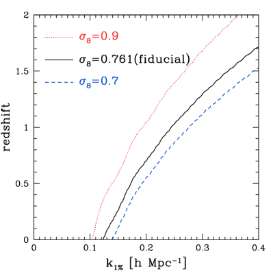
Figure 2 shows the numerical values of as a function of redshift. Here, in addition to the result for our fiducial cosmological model (solid), we also plot the results for the cases with slightly different amplitudes: (dashed) and (dotted), keeping the other remaining parameters fixed. The validity range of perturbation theory has a strong dependence on the redshift and the normalization. For the higher fluctuation amplitude with , the perturbation theory breaks down at a relatively smaller wave number.
3.3 Characterizing the acoustic oscillation scales
We are especially concerned with the systematic influences of the non-linear clustering and the redshift-space distortion on the characteristic scale of BAO, affecting its use as a cosmic standard ruler. To quantify the degree of these influences, we must first define the algorithm to characterize the oscillatory features from the power spectrum, by which the locations of peaks and the troughs are identified unambiguously. Then, the systematic influences can be investigated by measuring both the amplitude and the locations of peaks (and troughs). There are several approaches to separate the oscillatory pattern from the power-law behavior of power spectrum. In this paper, we study the following three methods:
- (i)
-
Divide the matter power spectrum by a smooth linear spectrum:
(28) where represents the “no-wiggles” approximation of the linear power spectrum given by Eisenstein & Hu (1998), which can be evaluated for our fiducial cosmological model. With this characterization, smooth power-law behavior in the power spectrum is effectively eliminated and the peaks and the troughs of acoustic oscillations are clearly identified. Note, however, that the above definition only corrects the power-law feature of the linear spectrum and non-linear corrections of power spectrum are left untouched in the numerator. Furthermore, there is uncertainty in the normalization of the amplitude.
- (ii)
-
Take the logarithmic derivative:
(29) In contrast to the method (i), this method is free from the uncertainty in the normalization of amplitude. Also, it automatically separate the smooth power-law feature of from the oscillatory behavior. In practice, however, it seems rather difficult in estimating the logarithmic derivative from the noisy binned data.
- (iii)
-
Divide the matter power spectrum by the smooth spectrum constructed from the matter power spectrum itself:
(30) This method is almost identical to the one proposed by Percival et al. (2007). Since we do not need a reference spectrum, it seems useful in characterizing the acoustic signature from the observed spectrum. Here, the smooth spectrum is constructed as follows. First we sample 70 data points from our perturbation spectrum between Mpc-1 and Mpc-1 with equal separation and without weight. Then we select nodes separated by Mpc-1 between Mpc-1 and Mpc-1, and an additional node at Mpc-1. Connecting the sample points by fitting cubic B-spline functions at each node, we obtain the smooth power spectrum .
Finally, evaluating the function in each method, we search for the local maxima and minima, which we respectively call peaks and troughs to characterize the sound horizon scales in BAOs:
| (31) |
As a reference, positions of peaks and troughs are computed in each method for the linear power spectrum and the resultant numerical values are listed in Table 1.
| method | 1st peak | 2nd peak | 3rd peak | 4th peak | 1st trough | 2nd trough | 3rd trough | 4th trough |
|---|---|---|---|---|---|---|---|---|
| (i) | 0.0669 | 0.1221 | 0.1792 | 0.2377 | 0.0415 | 0.0944 | 0.1500 | 0.2075 |
| (ii) | 0.0533 | 0.1074 | 0.1638 | 0.2216 | 0.0823 | 0.1368 | 0.1933 | 0.2514 |
| (iii) | 0.0663 | 0.1224 | 0.1788 | 0.2370 | 0.0417 | 0.0940 | 0.1506 | 0.2076 |
4 Baryon Acoustic Oscillations from perturbation theory
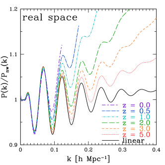
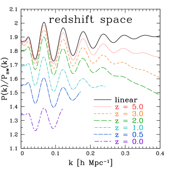
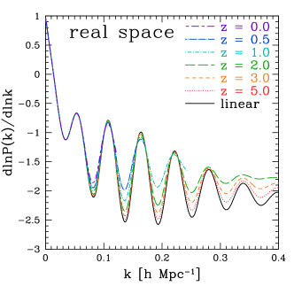
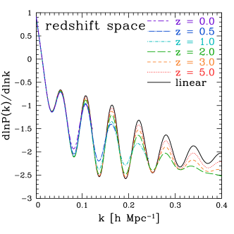
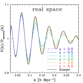
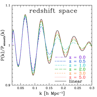
Now we are in a position to discuss the systematic effects on the BAOs by evaluating the functions . Consider first the general trends of the systematic influences. In figures 5, 5 and 5, redshift dependence of the functions is plotted against the wave number for three different methods. In each panel, solid lines represent the results from the linear theory prediction. Note here that the plotted curves from the perturbation results are all restricted to the range, , where the perturbation theory is safely applied (see Eq.[27]).
Basically, depending on the characterization methods, the non-linear clustering and the redshift-space distortion affect the characteristic scale of BAOs in very different manners. In figure 5, deviations from the linear theory prediction become more significant in both real and redshift spaces, as the redshift or scale decreases. While the growth of the amplitude is clearly seen in real space, the suppression of the amplitude is observed in redshift space, together with the overall shifts of acoustic oscillation. The latter effects are simply the outcome of the redshift-space distortion. By contrast, systematic effects on the amplitudes and , shown in figures 5 and 5, seem rather mild. A closer look at the BAO signal reveals that the oscillatory features tend to be erased as the redshift and the wavenumber increase. This trend has also been seen in -body simulations (Seo & Eisenstein, 2005; Angulo et al., 2007) and modeled by convolving the Gaussian filter with the linear power spectrum (e.g., Eisenstein et al. (2005)). Note that the Gaussian behavior in the disappearance of the oscillatory pattern is indeed suggested from the non-perturbative prediction based on the renormalized perturbation theory (Crocce & Scoccimarro 2006b). In the present analysis using the perturbation theory, the disappearance of the acoustic oscillation mainly comes from the one-loop terms , showing the monotonic behaviors as function of redshift and wave number.
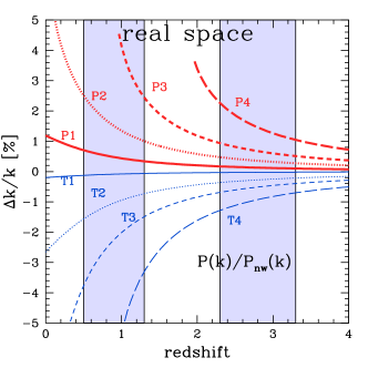
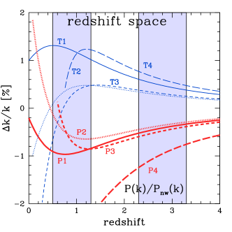
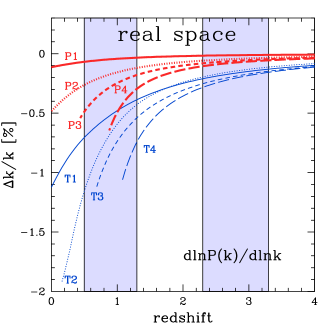
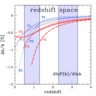
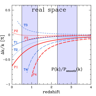
Turn next to focus on the systematic influences on the location of the peaks and the troughs. For this purpose, we define the fractional shift, , given by
| (32) |
and quantify the degree of the positional shifts in each method. Here, the quantities and represent the wave number of the peak (or trough) location calculated from the perturbation theory and the linear theory, respectively.
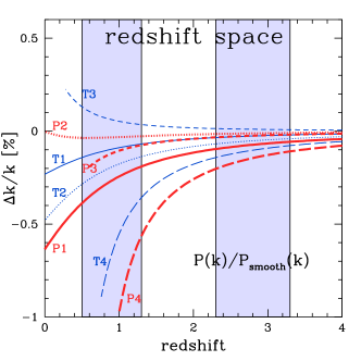
Figures 8, 8 and 8 show the fractional shifts of the peak and the trough positions measured from the three different methods, plotted as functions of redshift. In each panel, thick and thin lines respectively indicate the fractional shifts for the peaks (from P1 to P4) and the troughs (from T1 to T4). As a reference, we also plot the observational windows of the planned galaxy redshift survey, WFMOS, depicted as shaded regions. As anticipated from the general trends, the systematic changes in the peak and the trough positions become significant on small scales and at lower redshift. Also, quite naturally, the magnitude of the shift depends on the characterization algorithm. At the redshift around , the fractional shift of the peaks and the troughs reaches or exceeds % in cases using , while in the method , the systematic effects are reduced to % level. When translating these results to the measurement error of the sound horizon scales, the uncertainty in determining the equation of state parameter will amount to % for the method using , and to % for the method with (see Fig. 1). On the other hand, for the method with , a rather small value of the fractional shifts (less than %) is obtained. This is very good news for the precision measurement of sound horizon scales. The basic reason for the negligible shifts is originated from the definition (30) itself that the non-linear growth and the FOG effect are incorporated into both the numerator and the denominator, by which major sources for the peak and the trough shifts are effectively eliminated. As a consequence, the redshift dependence of the fractional shifts seen in the real space is almost identical to the one in the redshift space. By contrast, the characterization methods with or show different redshift dependence between real and redshift spaces. Interestingly, the behaviors of the fractional shifts seen in figure 8 show some symmetries between peaks and troughs. These systematic trends are related to the non-linear corrections arising from the gravitational clustering and the redshift-space distortion. We will discussed this issue in some detail in the next section.
5 A toy model for peak and trough shifts
The previous section reveals that both the non-linear clustering and the redshift-space distortion can lead to the physical shift of the peak and trough positions. However, their influences apparently depend on the characterization method for the BAO signals. In this section, we discuss how to understand the positional shifts by introducing a simple toy model.
Our primary goal is a qualitative understanding of the behaviors of the positional shift. Let us suppose that the acoustic signature in the linear theory prediction can be described by a simple sinusoidal function as
| (33) |
Of course, this is too naive an assumption, but the outcome of the following analysis still keeps the essence of our findings. From equation (33), the position of the peaks and the troughs, denoted by , satisfies the following relation:
| (34) |
Note that the peak (trough) implies that is even (odd) number. We then add the corrections due to the non-linear clustering and the redshift-space distortion, and discuss how the correction induces the positional shifts. Based on figures 5, 5 and 5, the non-linear corrections may be modeled by
| (35) |
In the above expression, the Gaussian factor represents the smoothing of the acoustic oscillations by the non-linear evolution. The function is assumed to be a monotonic function, which mimics the residuals that cannot be absorbed by taking logarithmic derivative and/or division by the smooth spectrum. Roughly speaking, monotonically increasing behavior of the function arises from the non-linear growth of gravitational clustering, while the monotonically decreasing behavior appears due to the FOG effect in redshift space. Note that the parameter and the function also depend on the redshift.
In the present analysis using perturbation theory, the corrections appearing in equation (35) should be small and perturbative treatment is always valid. We express the peak and the trough position by and the shift is treated as small quantity compared to the sound horizon scales, . From the definitions of peaks and troughs, we have (see Eq.[31]),
| (36) |
With a help of the relation (34), the above equation is reduced to the expression for the shift , the result of which is summarized as the fractional shift (see Eq.[32]):
| (40) |
where we have used the fact that and .
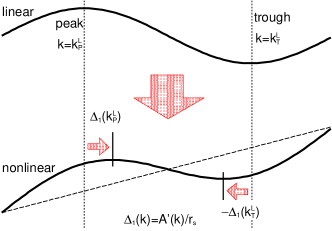
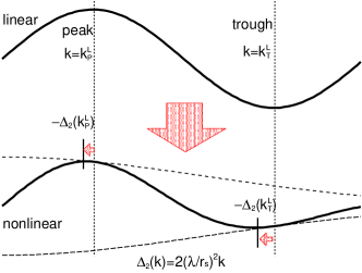
From equation (40), systematic changes in the positional shifts may be interpreted as a result of the two competing effects. The first term, arising from the Gaussian smoothing factor, always makes the position of peaks and troughs move toward smaller . On the other hand, the second term, coming from the monotonic behavior of the residual corrections, affects the positional shifts symmetrically: while the peak moves to the high- direction, the trough is shifted to a small . The magnitude of these trends will be illuminated more as non-linear corrections become important. In figure 9, the role of the two competitive effects are illustrated schematically.
Equation (40) qualitatively explains the behaviors seen in the previous section. In the case of the function , the growth or the suppression of amplitudes was significant and the smoothing effect of acoustic signature was sub-dominant (Fig. 5). As a result, the peaks and the troughs mutually move in an opposite direction, consistent with the toy model (40). A closer look at the late-time evolution in redshift space shows somewhat curious behavior that the time evolution of positional shift eventually changes its direction from smaller to larger for peaks, and from larger to smaller for troughs (Fig. 8). Perhaps, this might result from the imbalance of the two competitive effects: non-linear growth of gravitational clustering and suppression by the FOG effect. Hence, if we allow the sign of to change, this is also explained by the toy model (40). On the other hand, for the method using and , disappearance of acoustic oscillation is the major effect (see Figs. 5 and 5). Although the acoustic signature seen in the function is primarily declined, centered around , this does not essentially affect the positional shift. As a consequence, the position of the peaks and the troughs systematically moves to the low- direction. Again, we emphasize the remarkably small shift found in the function (Fig. 8). This implies that the corrections corresponding to the term are completely eliminated. Hence, with the characterization method , systematic error in the measurement of sound horizon scale would be greatly reduced, leading to an accurate determination of the equation of state parameter .
6 Conclusions
We have considered the shifts of the BAO characteristic scales due to the nonlinear gravitational and redshift-space distortion effects in a weakly nonlinear regime using one-loop correction from perturbation theory. We adopted three different methods to define the BAO oscillatory features from the entire power spectrum, and compute the shifts of peak and trough locations relative to the purely linear theory predictions in real space.
In doing so, we presented an analytic toy model to account for the physical reasons for the shifts, and showed that one particular method similar to the earlier proposal by Percival et al. (2007) is fairly free from the nonlinear and redshift-space distortion effects. In practice, the shifts of the first few peak and trough locations defined in the above procedure are at the level, ensuring precision in terms of the dark energy parameter , even if one uses the linear theory predictions as a standard ruler. Of course the shifts can be accurately computed using our methodology as long as the one-loop correction is dominant in the regime of interest.
The result is fairly robust against possible additional effects such as a weakly scale-dependent biasing and a running spectral index because they preferentially change the smoothed component in the power spectrum that is almost removed from the above procedure.
Of course the next task is to establish an accurate model that predicts the amplitude of the BAO under the nonlinear and redshift-space distortion effects. We suspect that it is very challenging given the limitation in both the current theoretical framework and numerical simulations. In particular, the nonlinear stochastic nature of the galaxy biasing seems problematic (e.g., Taruya (2000); Nishimichi et al. (2007)). It is still very difficult to incorporate this effect into theoretical predictions in any realistic and believable manner.
In light of this, it may be reasonable at this point to use the BAO scale information exclusively in constraining dark energy, ignoring its amplitude. In practice, constraints on cosmological parameters from the use of the BAO scale as a standard ruler hinges on the feasibility of the simultaneous fitting of the multiple BAO peaks and troughs. Furthermore, two-dimensional (line-of-sight and plane of the sky directions) features in redshift-space may improve the accuracy on the BAO scale. We are currently working on a simulation-based study, which is necessary to investigate these issues quantitatively.
We thank M. Takada, A. Nishizawa and E. Reese for useful comments related to the topic in the present paper. This work is supported in part by Japan Society for Promotion of Science (JSPS) Core-to-Core Program “International Research Network for Dark Energy”. T.N, A.S and K.Y acknowledge the support from the JSPS Research Fellows. A.T and K.Y are supported by a a Grant-in-Aid for Scientific Research from the JSPS (Nos. 18740132, 18540277, 18654047).
Appendix A The linear theory prediction of the characteristic scales
The BAO characteristic scale imprinted in the matter power spectrum is basically the sound horizon scale at recombination, (eq.[3]). Depending on the specific definitions of peaks and troughs in -space that we adopted here, however, their corresponding scales are slightly different from the value of equation (3), which has a non-negligible effect in estimating the cosmological parameters. The purpose of this Appendix is to clarify the difference in linear theory predictions.
The observed BAO scale in real space is expected to differ slightly from due to the residual baryon-photon interaction after recombination (). Eisenstein & Hu (1998) pointed out that a more accurate value is given simply by replacing the with the drag epoch :
| (A41) |
where is the ratio of the baryon to photon momentum densities at . Equation (A41) implies that Mpc, which is about 5% larger than Mpc.
The characteristic scale in k-space is even more subtle. So let us first model the oscillating part of baryon transfer function as
| (A42) |
If we adopt equation (3), the phase is written as
| (A43) |
Eisenstein & Hu (1998) took into account of baryon density perturbation at the drag epoch itself, which changes the phase at large scales where the velocity overshoot is not the dominant effect. As a result, they found that the phase is approximated as
| (A44) |
where
| (A45) | |||||
| (A46) |
In these expressions, the characteristic scales in space are defined through
| (A47) |
where for peaks for troughs from our methods (i) and (iii). In contrast, our method (ii) implies that for peaks for troughs.
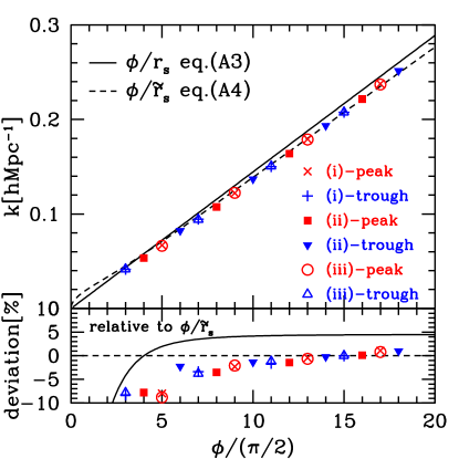
Figure 10 compares those theoretical predictions with our peak and trough positions in Table 1 (computed using CAMB). The upper panel shows the relation between the phase and the wavenumber ; the solid and dashed lines are calculated using equation (A43) and (A44), respectively. The symbols denote our results for peaks and troughs with the three methods listed in Table 1. We also plot the fractional deviation with respect to equation (A44) in the lower panel.
The solid and dashed lines suggest that equations (A43) and (A44) are indeed different by 5% as expected. This is crucial since the difference propagates to 20% in . The dashed line fits our CAMB results (symbols) very well for , which ensures the validity of the formula of Eisenstein & Hu (1998). Nevertheless our results for the first few peaks and troughs are systematically different from their fitting formula (the lower panel of Figure 10). This would simply reflect the difference of our definitions of the peaks and troughs with respect to theirs, which one should keep in mind when performing an actual statistical analysis of real datasets.
Appendix B Kernels for perturbative solution and one-loop power spectrum
Here, we briefly summarize the kernels for perturbative solutions presented in equation (15) and present the explicit expressions for the one-loop power spectrum (see Eqs.[19] and [20]).
In the Einstein-de Sitter universe, the kernel satisfies the following recursion relation (Goroff et al., 1986):
| (B1) | |||
| (B2) |
where , , , and
| (B5) |
From these relations, one obtains the symmetrized kernels, (density part) and (velocity part) (e.g., Jain & Bertschinger (1994)):
| (B6) |
| (B7) |
| (B8) | |||||
| (B9) | |||||
The explicit expressions for one-loop correction terms in equations (19) and (20) are (e.g., Makino, Sasaki & Suto (1992))
| (B10) | |||||
| (B11) | |||||
for the power spectrum of density field,
| (B12) | |||||
| (B13) | |||||
for the cross power spectrum of density and velocity divergence, and
| (B14) | |||||
| (B15) | |||||
for the power spectrum of velocity divergence.
References
- Angulo et al. (2005) Angulo, R., et al., 2005, MNRAS, 362, 25
- Angulo et al. (2007) Angulo, R. Baugh, C. M., Frenk, C. S., & Lacey, C. G., 2007, MNRAS, submitted, astro-ph/0702543
- Ballinger, Peacock & Heavens (1996) Ballinger, W. E., Peacock, J. A., & Heavens, A. F., 1996, MNRAS, 282, 877
- Bernardeau et al. (2002) Bernardeau, F., Colombi, S., Gaztañaga, E., and Scoccimarro, R., 2002, Phys. Rep., 367, 1
- Bernardeau (1994) Bernardeau, F., 1994, ApJ, 433, 1
- Blake & Glazebrook (2003) Blake, C., & Glazebrook, K., 2003, ApJ, 594, 665
- Chodorowski & Ciecielag (2002) Chodorowski, M. J., & Ciecielag, P., 2002, MNRAS, 331, 133
- Cole, Fisher & Weinberg (1994) Cole, S., Fisher, K. B., & Weinberg, D. H., 1994, MNRAS, 267, 785
- Cole et al. (2005) Cole, S., et al., 2005, MNRAS, 362, 505
- Crocce & Scoccimarro (2006a) Crocce, M., & Scoccimarro, R., 2006a, Phys. Rev. D, 73, 063519
- Crocce & Scoccimarro (2006b) Crocce, M., & Scoccimarro, R., 2006b, Phys. Rev. D, 73, 063520
- Crocce & Scoccimarro (2007) Crocce, M., & Scoccimarro, R., 2007, arXiv:0704.2783
- Eisenstein & Hu (1998) Eisenstein, D. J., & Hu, W., 1998, ApJ, 496, 605
- Eisenstein et al. (2005) Eisenstein, D. J., et al., 2005, ApJ, 633, 560
- Eisenstein, Seo & White (2006) Eisenstein, D. J., Seo, H. J., & White, M. 2006, ApJ, submitted, astro-ph/0604361
- Eisenstein et al. (2006) Eisenstein, D. J., Seo, H. J., Sirko, E., & Spergel, D., 2006, ApJ, submitted, astro-ph/0604362
- Fry (1984) Fry, J. N., 1984, ApJ, 279, 499
- Goroff et al. (1986) Goroff, M. H., Grinstein, B., Rey, S. J., & Wise, M. B. 1986 ApJ, 311, 6
- Guzik, Bernstein & Smith (2007) Guzik, J., Bernstein, G., & Smith, R. E., 2007, MNRAS, 375, 1329
- Hütsi (2006) Hütsi, G., 2006, A&A, 449, 891
- Jain & Bertschinger (1994) Jain, B., & Bertschinger, E., 1994, ApJ, 431, 495
- Jeong & Komatsu (2006) Jeong, D., & Komatsu, E., 2006, ApJ, 651, 619
- Juszkiewicz (1981) Juszkiewicz, R., 1981, MNRAS, 197, 931
- Kaiser (1987) Kaiser, N., 1987, MNRAS, 227, 1
- Lewis, Challinor & Lasenby (2000) Lewis, A., Challinor, A., & Lasenby, A., 2000, ApJ, 538, 473
- Ma (2006) Ma, Z., 2006, ApJ, accepted, astro-ph/0610213
- Magira, Jing & Suto (2000) Magira, H., Jing, Y. P., & Suto, Y., ApJ, 528, 30
- Meiksin, White & Peacock (1999) Meiksin, A., White, M., & Peacock, J. A., 1999, MNRAS, 304, 851
- Makino, Sasaki & Suto (1992) Makino, N., Sasaki, M., & Suto, Y., 1992, Phys. Rev. D, 46, 585
- Matarrese & Pietroni (2007a) Matarrese, S., & Pietroni, M., 2007a, astro-ph/0702653
- Matarrese & Pietroni (2007b) Matarrese, S., & Pietroni, M., 2007b, astro-ph/0703563
- Matsubara (1995) Matsubara, T., 1995, Prog. Theor. Phys., 94, 1151
- McDonald (2007) McDonald, P., 2006, Phys. Rev. D, 75, 043514
- Nishimichi et al. (2007) Nishimichi, T., et al., 2007, PASJ, 59, 93
- Padmanabhan & Ray (2006) Padmanabhan, T., & Ray, S., 2006, MNRAS, 372, 53
- Padmanabhan et al. (2006) Padmanabhan, N., et al., 2006, MNRAS, submitted, astro-ph/0605302
- Park et al. (1994) Park, C., Vogeley, M. S., Geller, M. J., & Huchra, J. P., 1994, ApJ, 431, 569
- Peacock & Dodds (1994) Peacock, J. A., & Dodds, S. J., 1994, MNRAS, 267, 1020
- Percival et al. (2007) Percival. W., et al., 2007, ApJ, 657, 51
- Scoccimarro et al. (1998) Scoccimarro, R., Colombi, S., Fry, J. N., Frieman, J. A., Hivon, E., & Melott, A. 1998, ApJ, 496, 586
- Scoccimarro (2001) Scoccimarro, R. 2001, NYASA, 927, 13
- Scoccimarro (2004) Scoccimarro, R., 2004, Phys. Rev. D, 70, 083007
- Seo & Eisenstein (2003) Seo, H. J., & Eisenstein, D. J., 2003, ApJ, 598, 720
- Seo & Eisenstein (2005) Seo, H. J., & Eisenstein, D. J., 2003, ApJ, 633, 575
- Shirata et al. (2005) Shirata, A., Shiromizu, T., Yoshida, N., & Suto, Y., 2005, Phys. Rev. D, 71, 064030
- Smith, Scoccimarro & Sheth (2007a) Smith, R. E., Scoccimarro, R., & Sheth, R. K., 2007a, Phys. Rev. D, 75, 063512
- Smith, Scoccimarro & Sheth (2007b) Smith, R. E., Scoccimarro, R., & Sheth, R. K., 2007b, astro-ph/0703620
- Spergel et al. (2007) Spergel, D. N., et al., 2007, ApJS, 170, 377
- Springel et al. (2005) Springel, V., et al., 2005, Nature, 435, 629
- Suto & Sasaki (1991) Suto, Y., & Sasaki, M., 1991, Phys. Rev. Lett., 66, 294
- Taruya (2000) Taruya, A., 2000, ApJ, 537, 37
- Tegmark et al. (2006) Tegmark, M., et al., 2006, Phys. Rev. D, 74, 123507
- Valageas (2007) Valageas, P., 2007, A&A, 465, 725
- Vishniac (1983) Vishniac, E., 1983, MNRAS, 203, 345
- Yamamoto et al. (2006) Yamamoto, K., Bassett, B. A., Nichol, R. C., Suto, Y., & Yahata, K., 2006, Phys. Rev. D, 74, 063525