Composite Interstellar Grains

Abstract

A composite dust grain model which is consistent with the observed interstellar extinction and linear polarization is presented. The composite grain is made up of a host silicate spheroid and graphite inclusions. The extinction efficiencies of the composite spheroidal grains for three axial ratios are computed using the discrete dipole approximation (DDA). The interstellar extinction curve is evaluated in the spectral region 3.40–0.10$\mu m$ using the extinction efficiencies of the composite spheroidal grains. The model extinction curves are then compared with the average observed interstellar extinction curve. We also calculate the linear polarization for the spheroidal composite grains at three orientation angles and find the wavelength of maximum polarization. Further, we estimate the volume extinction factor, an important parameter from the point of view of cosmic abundance, for the composite grain models that reproduce the average observed interstellar extinction. The estimated abundances derived from the composite grain models for both carbon and silicon are found to be lower than that are predicted by the bare silicate/graphite grain models but these values are still higher than that are implied from the recent ISM values.

1 Introduction

The most commonly used interstellar dust grain model, consists of two distinct populations of bare spherical silicate and graphite grains with a power law size distribution (Mathis et al. 1977) . This model, popularly known as MRN model provides an excellent fit to the average observed interstellar extinction curve. However, it is highly unlikely that the interstellar grains are spherical in shape or that they are homogeneous in composition and structure. The collected interplanetary particles are nonspherical and highly porous and composites of very small sub-grains glued together (Brownlee, 1987). Moreover, the interstellar polarization that accompanies extinction requires that the interstellar grains must be aligned and nonspherical (Wolff et. al. 1993). Recently Stark et al. (2006) have suggested the growth of spheroidal grains via plasma deposition in the supernova remnant. The elemental abundances derived from the observed interstellar extinction also do not favour the homogeneous composition for the interstellar grains. Recent studies suggest that the abundances of various elements in the interstellar medium (ISM) are less than their solar values (Snow & Witt, 1996; Voshchinnikov et al., 2006). For example in case of carbon, its solar abundance normalized to a hydrogen abundance of $10^{6}$ atoms, is about 355 (Grevesse et al. 1996). In the ISM the abundance of this element is significantly lower, about 225 C atoms (Snow & Witt 1995). Also a significant amount of this interstellar carbon is in gas phase. From CII 2325Å  absorption measurements, Cardelli et al. (1996) have inferred a C abundance of about 150 atoms . This means that a total of about 100 C atoms are available for the dust phase, compared with about 300 atoms required for the bare grain models (e.g. Mathis et al. 1977, MRN). In order to overcome the cosmic abundance constraints Mathis & Whiffen (1989), Mathis (1996) and Dwek (1997) have proposed composite grain models consisting of silicate and amorphous carbon as constituent materials. They have used effective medium theory (EMT) to calculate the optical constants for composite grains and then used the Mie theory to calculate extinction cross sections for spheres In EMT the inhomogeneous particle is replaced by a homogeneous one with some ’average effective dielectric function’. The effects related to the fluctuations of the dielectric function within the inhomogeneous structures cannot be treated by this approach of the EMT. Mathis (1996) has also noted the uncertainty in the use of EMT for treating the composite grains and has suggested that detailed calculations such as the DDA would be necessary for the treatment of voids in silicate/graphite particles for some wavelengths.

Iati et al. (2004) have studied optical properties of composite grains as grain aggregates of amorphous carbon and astronomical silicates, using the transition matrix approach. Voshchinnikov et al. (2005) have studied properties of composite grains as layered spheres. Very recently Voshchinnikov et al. (2006) have studied the effect of grain porosity on interstellar extinction, dust temperature, infrared bands and millimeter opacity. They have used both, the EMT-Mie based calculations and layered sphere model.

We have used discrete dipole approximation (DDA) to study the extinction properties of the composite grains. For the description on the DDA see Draine (1988). The DDA allows the consideration of irregular shape effects, surface roughness and internal structure within the grain (Wolff et al. 1994, 1998 and Voshchinnikov et al. 2005). For discussion and comparison of DDA and EMT methods, including the limits of the effective medium theory, see Bazell and Dwek (1990), Perrin and Lamy (1990), Perrin and Sivan (1990), Ossenkopf (1991) and Wolff et al (1994). In our earlier study we had used composite spherical grain models to evaluate the interstellar extinction curve in the wavelength range 0.55–0.20$\mu m$ (Vaidya et.al. 2001).

In the present study, we use more realistic composite spheroidal grain models and calculate the extinction efficiencies in the extended wavelength region, 3.40–0.10$\mu m$ and linear polarization in the visible - near infrared region, i.e. 0.35–1.00$\mu m$.

Using these extinction efficiencies of the composite grains with a power law type grain size distribution we evaluate the interstellar extinction curve and linear polarization. In addition to reproducing the observed interstellar extinction curve, the grain model should also be consistent with the abundance constraints. We estimate the volume extinction factor, an important parameter from the point of view of the cosmic abundance, for the composite grain models that reproduce the average observed extinction. In section 2 we give the validity criteria for the DDA and the composite grain models. In section 3 we present the results of our computations and discuss them. The main conclusions of our study are given in section 4.

2 Discrete Dipole Approximation (DDA) and Composite grains

The basic DDA method consists of replacing a particle by an array of N oscillating polarizable point dipoles (Draine, 1988). The dipoles are located on a lattice and the polarizability is related to the complex refractive index $m$ through a lattice dispersion relationship (Draine & Goodman, 1993). Each dipole responds to the external electric field as well as to the electric field of the other N-1 dipoles that comprise the grain. The polarization at each dipole site is therefore coupled to all other dipoles in the grain.

In the present study, we have used the ddscat6.1 code (Draine & Flatau, 2003) which has been modified and developed by Dobbie (1999) to generate the composite grain models. The code, first carves out an outer sphere (or spheroid) from a lattice of dipole sites. Sites outside the sphere are vacuum and sites inside are assigned to the host material. Once the host grain is formed, the code locates centers for internal spheres to form inclusions. The inclusions are of a single radius and their centers are chosen randomly. The code then outputs a three dimensional matrix specifying the material type at each dipole site which is then received by the ddscat program. In the present case, the sites are either silicates, graphite or vacuum.

Using the modified code, we have studied composite grain models with a host silicate spheroid containing number of dipoles N=9640, 25896 and 14440, each carved out from $32\times 24\times 24$, $48\times 32\times 32$ and $48\times 24\times 24$ dipole sites, respectively; sites outside the spheroid are set to be vacuum and sites inside are assigned to be the host material. It is to be noted that the composite spheroidal grain with N=9640 has an axial ratio of 1.33, whereas N=25896 has the axial ratio 1.5, and N=14440 has the axial ratio 2.0. The volume fractions of the graphite inclusions used are 10%, 20% and 30% (denoted as f=0.1, 0.2 and 0.3) Details on the computer code and the corresponding modification to the ddscat code (Draine & Flatau 2003) are given in Dobbie (1999), Vaidya et al. (2001) and Gupta et al. (2006). Figure 1 and 2 illustrate the composite grain model with number of dipoles N=9640 for the host spheroid and eleven inclusions.

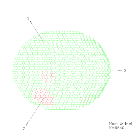
Figure 1: A typical non-spherical composite grain with a total of N=9640 dipoles where the inclusions embedded in the host spheroid are shown such that only the ones placed at the outer periphery are seen.

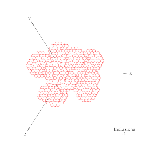
Figure 2: Same as Fig. 1 but shows the inclusions.

Table 1 shows the number of dipoles for each grain model (first column), number of dipoles per inclusion with the number of inclusions denoted in bracket for volume fraction f=0.1 (second column). The third and fourth column are the corresponding values for the remaining volume fractions i.e. f=0.2 and 0.3.

Table 1: Number of dipoles for each inclusion for the three model

No. of Dipoles(Axial ratio)	f=0.1	f=0.2	f=0.3
N=9640(1.33)	152(6)	152 (11)	152(16)
N=25896(1.50)	224(6)	224 (11)	224(16)
N=14440(2.00)	432(7)	432 (13)	432(19)

There are two validity criteria for DDA (see e.g. Wolff et al. 1994); viz. (i) $\rm|m|kd\leq 1$, where m is the complex refractive index of the material, k=$\rm\pi/\lambda$ is the wavenumber and d is the lattice dispersion spacing and (ii) d should be small enough (N should be sufficiently large) to describe the shape of the particle satisfactorily. The complex refractive indices for silicates and graphite are obtained from Draine (1985, 1987). For any grain model, the number of dipoles required to obtain a reliable computational result can be estimated using the ddscat code (see Vaidya & Gupta 1997 and 1999, Vaidya et al. 2001). For the composite grain model, if the host grain has N dipoles, its volume is N(d)³ and if ’a’ is the radius of the host grain , N(d)³=4/3$\rm\pi(a)^{3}$, hence, N=4$\rm\pi/3(a/d)^{3}$, and if $\rm|m|kd\leq 1$ and k=$\rm\pi/\lambda$ the number of dipoles N can be estimated at a given wavelength and the radius of the host grain. For all the composite grain models, with N=9640, 25896 and 14440 and for all the grain sizes, between a=0.001–0.250$\mu$, in the wavelength range of 3.40–0.10$\mu m$, considered in the present study; we have checked that the DDA criteria are satisfied.

Table 2 shows the maximum grain size ’a’ that satisfies the DDA validity criteria at several wavelengths for the composite grain models with N=9640, 14440 and 25896.

Table 2: DDA validity criteria

$\lambda$ ($\mu m$)	N=9640	14440	25896
	a($\mu$)	a($\mu$)	a($\mu$)
3.4000	4.00	5.00	6.00
2.2000	2.50	3.50	4.00
1.0000	1.20	1.40	1.60
0.7000	0.80	1.20	1.00
0.5500	0.60	0.96	0.80
0.3000	0.40	0.50	0.45
0.2000	0.22	0.30	0.25
0.1500	0.14	0.20	0.16
0.1000	0.10	0.16	0.12

It must be noted here that the composite spheroidal grain models with N=9640, 25896 and 14440 have the axial ratio 1.33, 1.5 and 2.0 respectively and if the semi-major axis and semi-minor axis are denoted by x/2 and y/2 respectively, then $\rm a^{3}=(x/2)(y/2)^{2}$, where where ’a’ is the radius of the sphere whose volume is the same as that of a spheroid. In order to study randomly oriented spheroidal grains, it is necessary to get the scattering properties of the composite grains averaged over all of the possible orientations; in the present study we use three values for each of the orientation parameters ($\rm\beta,\theta and\phi$), i.e. averaging over 27 orientations, which we find quite adequate (see e.g. Wolff et al. 1998).

3 Results

3.1 Extinction Efficiency of Composite Spheroidal Grains

Earlier, we had studied the extinction properties of composite grains made up of the host spherical silicate grains with graphite inclusions in the limited wavelength region 0.55–0.20$\mu m$ (Vaidya et al. 2001). However, since the observed interstellar polarization requires that the interstellar grains must be nonspherical, in the present paper we study the extinction properties and linear polarization of the composite spheroidal grains with three axial ratios, viz. 1.33, 1.5 and 2.0, corresponding to the grain models with number of dipoles N=9640, 25896 and 14440 respectively, for three volume fractions of inclusions; viz. 10%, 20% and 30%, in the extended wavelength region 3.40–0.10$\mu m$.

Figures 3 (a-f) show the extinction efficiencies ($\rm Q_{ext}$) for the composite grains with the host silicate spheroids containing 9640, 25896 and 14440 dipoles, corresponding to axial ratio 1.33, 1.5 and 2.0 respectively. The three volume fractions, viz. 10%, 20% and 30%, of graphite inclusions are also listed in the top (a) panel. The radius of the host composite grain is set to 0.01$\mu$ for all the cases. The extinction in the spectral region 0.55–0.20$\mu m$ is highlighted in the panels (d), (e) and (f).

Figure 3: Extinction Efficiencies for the composite grains of size 0.01$\mu$ with host spheroids containing dipoles N=9640, 25896 and 14440 are shown in (a),(b) and (c) in the wavelength region, 3.40–0.10$\mu m$. The panels (d),(e) and (f) show the extinction curves in the wavelength region 0.55–0.20$\mu m$.

The effect of the variation of volume fraction of inclusions is clearly seen for all the models. The extinction efficiency increases as the volume fraction of the inclusion increases. It is to be noted that the wavelength of the peak extinction shifts with the variation in the volume fraction of inclusions. These extinction curves also show the variation in the width of the extinction feature with the volume fraction of inclusions. All these results indicate that the inhomogeneities within the grains play an important role in modifying the ’2175Å ’ feature. Voshchinnikov (1990) and Gupta et al. (2005) had found variation in the ’2175Å ’ feature with the shape of the grain, and Iati et al. (2001, 2004); Voshchinnikov (2002); Voshchinnikov and Farafonov (1993) and Vaidya et al. (1997, 1999) had found the variation in the feature with the porosity of the grains. Draine & Malhotra (1993) have found relatively little effect on either the central wavelength or the width of the feature for the coagulated graphite silicate grains.

We have also computed the extinction efficiencies of the composite spheroidal grains using the EMT-T-matrix based calculations. These results are displayed in Figures 4 (a-c). For these calculations, the optical constants were obtained using the Maxwell-Garnet mixing rule (i.e. effective medium theory, see Bohren and Huffman 1983). Description of T-matrix method/code is given by Mishchenko (2002). The extinction curves obtained using the EMT-T-matrix calculations, deviate from the extinction curves obtained using the DDA, particularly in the ’bump region’, i.e. 0.55–0.20$\mu m$. In Figures 5 (a-c) we have plotted the ratio Q(EMT)/Q(DDA) to compare the results obtained by both methods. The results based on the EMT-T-matrix calculations and DDA results do not agree because the EMT does not take into account the inhomogeneities within the grain; (viz. internal structure, surface, voids) (see Wolff et al. 1994, 1998) and material interfaces and shapes are smeared out into a homogeneous ’average mixture’ (Saija et al. 2001). However, it would still be very useful and desirable to compare the DDA results for the composite grains with those computed by other EMT/Mie type/T matrix techniques in order to examine the applicability of several mixing rules. (see Wolff et al. 1998, Voshchinnikov and Mathis 1999, Chylek et al. 2000, Voshchinnikov et al. 2005, 2006). The application of DDA, poses a computational challenge, particularly for the large values of the size parameter X ($\rm=2\pi a/\lambda>20$ ) and the complex refractive index m of the grain material would require large number of dipoles and that in turn would require considerable computer memory and cpu time (see e.g. Saija et al. 2001, Voshchinnikov et al. 2006).

Figure 4: Extinction Efficiencies for the composite spheroidal grains of size 0.01$\mu$ with three axial ratios (AR=1.33, 1.5 and 2.0) using EMT-T Matrix based calculations in the wavelength region 3.4–0.10$\mu m$.

Figure 5: Ratio Q(EMT-Tmatrix)/Q(DDA) in the wavelength region 0.55-0.20$\mu m$ for the composite spheroidal grains of size 0.01$\mu$ with three axial ratios, AR=1.33, 1.5, 2.0 corresponding to N=9640, 25896 and 14440 respectively.

Mathis & Whiffen (1989), Mathis (1996) and Voshchinnikov et al. (2006) in their composite grain models have used amorphous carbon with silicate. We have not considered it in the present study as amorphous carbon particles exhibit absorption at approximately 2500Å  and also it is highly absorbing at very long wavelengths and would provide most of the extinction longward of 0.3$\mu m$ (Draine 1989, Weingartner and Draine 2001). It is also not favoured by Zubko et al. (2004). Instead, large PAH molecules are likely candidates to be the carrier of the interstellar 2175Å  feature – a natural extension of graphite hypothesis (Draine, 2003b).

Figures 6(a-d) show the extinction efficiencies ($\rm Q_{ext}$) for the composite grains for four host grain sizes: viz. a=0.01, 0.05, 0.1 and 0.2 $\mu$ at a constant volume fraction of inclusion of 20%.

It is seen that the extinction and the shape of the extinction curves varies considerably as the grain size increases. The ’2175Å  feature’ is clearly seen for small grains ; viz. a=0.01 and 0.05$\mu$, whereas for larger grains the feature almost disappears. It is also to be noted that there is no appreciable variation in the extinction with the axial ratio of spheroidal grains; i.e. 1.33, 1.5, 2.0 corresponding to N=9640, 25896 and 14440.

Figure 6: Extinction efficiencies for the composite grains with various sizes with 20% volume fraction of graphite inclusions.

3.2 Interstellar Extinction Curve

The interstellar extinction curve (i.e. the variation of extinction with wavelength) is usually expressed by the ratio $\rm E(\lambda-V)/E(B-V)$ versus $1/\lambda$. We use the extinction efficiencies of the composite grains, with a power law size distribution (i.e. $\rm n(a)\sim a^{-3.5}$, Mathis et al. 1977) to evaluate the interstellar extinction curve in the wavelength region of 3.40–0.10$\mu m$. In addition to the composite grains a separate component of small graphite grains is required to produce the observed peak at 2175Å  in the interstellar extinction curve (Mathis, 1996). It must also be mentioned here that the most widely accepted explanation of the 2175Å  bump has been the extinction by small ($\sim a<0.05\mu$) graphite grains (e.g. Hoyle and Wickramasinghe 1962, Mathis et al. 1977, Draine 1989). Also, the stability of the observed feature at 2175Å  along all the lines of sight rules out the possibility of using composite grains, made up of silicate with graphite as inclusions to reproduce the feature. (Iati et al. 2001).

The average observed interstellar extinction curve (Savage and Mathis 1979; Whittet, 2003) is compared with with the model curve formed from a $\chi^{2}$ minimized and best fit linear combination of the composite grains (contributory fraction x) and graphite grains (contributory fraction y); i.e the model interstellar extinction curves for the composite grains and the graphite grains are linearly combined to render a net curve for comparison with the average observed extinction curve. The formula to obtain the minimized $\chi^{2}$ values is given by Bevington (1969).

$${\chi{{}^{2}_{j}}}=\frac{\sum_{i=1}^{n}(S_{i}^{j}-T_{i}^{k})^{2}}{pp}$$

where pp is the degrees of freedom, $S_{i}^{j}(\lambda_{i})$ is the $j$th model curve for the corresponding $x$ and $y$ linear combination of composite and graphite grains and $T_{i}^{k}(\lambda_{i})$ is for the observed curve, $\lambda_{i}$ are the wavelength points with i=1,n where n are the number of wavelength points of the extinction curves. Details are given in our earlier papers (see Vaidya & Gupta 1999, Vaidya et al. 2001).

Table 3 shows the best fit $\chi^{2}$ values for the extinction curves for the composite grain models with volume fraction of inclusions f=0.1, 0.2, 0.3 for three wavelength ranges, viz. 3.40–0.10$\mu m$, 3.40–0.55$\mu m$ and 0.55–0.20$\mu m$. The numbers in the brackets (x/y) adjacent to each $\chi^{2}$ value is the fractional contibution of the composite Si+f*Gr and the required additional small graphite grain e.g. (0.5/0.3) means that there is 0.5 contribution from the composite grain and 0.3 contribution from this additional graphite grain to obtain the corresponding minimum $\chi^{2}$ value.

Table 3: Best fit $\chi^{2}$ values for the Interstellar Extinction Curves for the Composite Spheroidal grain models in the wavelength range 3.40–0.10$\mu m$, 3.40–0.55$\mu m$ and 0.55–0.20$\mu m$ with grain size distribution a=0.005–0.250$\mu$. The numbers in the brackets adjacent to each $\chi^{2}$ value is the fractional contibution of the composite Si+f*Gr and the required additional small graphite grain.

Vol. fraction	N=9640	N=25896	N=14440
Wavelength range	3.40–0.10$\mu m$
f=0.1	0.1635(0.5/0.3)	0.1811(0.5/0.3)	0.1659(0.5/0.3)
f=0.2	0.2045(0.5/0.3)	0.2483(0.5/0.3)	0.1839(0.5/0.3)
f=0.3	0.3053(0.5/0.3)	0.4532(0.5/0.3)	0.3115(0.5/0.3)
Wavelength range	3.40–0.55$\mu m$
f=0.1	0.0148(0.5/0.3)	0.0148(0.6/0.2)	0.0176(0.5/0.3)
f=0.2	0.0273(0.7/0.1)	0.0352(0.6/0.1)	0.0306(0.7/0.1)
f=0.3	0.0360(0.6/0.1)	0.0570(0.6/0.1)	0.0400(0.6/0.1)
Wavelength range	0.55–0.20$\mu m$
f=0.1	0.0672(0.4/0.4)	0.0899(0.4/0.4)	0.0766(0.6/0.3)
f=0.2	0.1192(0.3/0.4)	0.1578(0.3/0.4)	0.1028(0.4/0.4)
f=0.3	0.1376(0.3/0.4)	0.1658(0.3/0.4)	0.1364(0.4/0.4)

Figure 7 shows the interstellar extinction curves for the composite grain models with number of dipoles for the host spheroids N=9640, 25896 and 14440 and volume fractions of inclusions f=0.1, 0.2 and 0.3 in the entire wavelength region of 3.40–0.10$\mu m$ for the power law grain size distribution, $\rm n(a)\sim a^{-3.5}$, in the size range, a=0.005–0.250$\mu$.

Figure 7: Comparison of the observed interstellar extinction curve with the best fit model combination curve of composite grains with three volume fractions of graphite inclusions (N=9640, 25896 and 14440) and graphite grains in the wavelength range of 3.40–0.10$\mu m$.

It is seen from Figure 7 and Table 3 that the composite spheroidal grain models with N=9640 and f=0.1 fit the average observed extinction curve quite satisfactorily in the entire wavelength range considered, i.e 3.40–0.10$\mu m$, in this study The model extinction curves with N=25896, 14440 deviate from the observed extinction curve in the uv region, i.e. beyond the wavelength $\sim$ 0.1500$\mu m$ (i.e. 6$\mu m^{-1}$). These results indicate that in addition to composite grains and graphite, a third component of very small grains (e.g very small silicate grains or PAHs) may be required to explain the extinction beyond 1500Å  in the UV (Weingartner and Draine, 2001).

Figure 8 shows the extinction curves in the wavelength range 0.55–0.20$\mu m$ for the composite grain models. It is seen that all the model curves fit quite well with the observed interstellar extinction curve in this wavelength region. $\chi^{2}$ values are also quite low in this region (see Table 3).

Figure 8: Comparison of the observed interstellar extinction curve with the best fit model combination curve of composite grains (N=9640, 25896 and 14440) and graphite grains in the wavelength range of 0.55–0.20$\mu m$.

We have also evaluated extinction curves for the smaller size range, viz. a=0.001–0.100$\mu$, so that the DDA validity criteria is satisfied for the grain models with N=9640 in the uv spectral region (see Table 2). Figure 9 shows the interstellar extinction curves for the composite grain models with N=9640 in the size range a=0.001–0.100$\mu$. The $\chi^{2}$ values for these model curves are 0.0908, 0.1094 and 0.1425 for the volume fractions f=0.1, 0.2 and 0.3 respectively.

Figure 9: Extinction curves for composite grain models with N=9640 for the size range, a=0.001–0.100$\mu$

These results show that the composite spheroidal grain models with the axial ratio of the host silicate spheroid not very large; i.e $\sim 1.33$, N=9640 and the volume fraction of the graphite inclusions, f=0.1 fit the observed extinction satisfactorily in the entire wavelength range 3.40–0.10$\mu m$, whereas in the wavelength range 0.55–0.20$\mu m$, all the composite spheroidal grain models with N=9640, 25896 and 14440 fit the observed extinction curve better and the $\chi^{2}$ values are lower.

Zubko et al. (1996, 1998) have used multicomponent mixtures of bare spherical grains to analyze the interstellar extinction curves. They have used the method of regularization for this analysis. Recently Iati et al. (2004), Zubko et al. (2004) Voshchinnikov et al. (2005) and Maron & Maron (2005) have also proposed composite grain models. However, all these authors have used EMT to obtain the optical constants for the composite grain models. Andersen et al. (2002) have performed extinction calculations for clusters of polycrystalline graphite and silicate spheres, using discrete dipole approximation. Very recently Voshchinnikov et al. (2006) have used both EMT-Mie type and layered sphere based calculations for the composite porous grain models. Voshchinnikov et al. (2006) have found the model extinction curves obtained using layered sphere based calculations fit the observed extinction better.

3.3 Linear Polarization

The linear polarization curve, usually plotted as $\rm P_{\lambda}$ versus $1/\lambda$, displays a broad peak in the visible region for most stars and the wavelength of maximum polarization $\rm\lambda_{max}$, varies from star to star, with a mean value at around 0.55$\mu m$. The dependence of the linear polarization on the wavelength is described by the empirical formula (Serkowski et al. 1975, Whittet 2003);

$\rm P_{\lambda}/P_{max}=exp[-Kln^{2}(\lambda/\lambda_{max})]$

where $\rm P_{max}$ is the degree of polarization at the peak, and the parameter K, determines the width of the peak. This formula with K=1.15 provides an adequate representation of the observations of interstellar polarization in the visible-NIR region (0.36–1.00$\mu m$) (Whittet et al. 1992). It is also important to note that the wavelength dependence of interstellar polarization is a function not only of the size, shape and composition of the dust grain but also of orientation of the grains (see e.g. Wolff et al. 1993).

Using ddscat (Draine and Flatau 2003) we have calculated linear polarization efficiency, $\rm|Q_{pol}|=Q_{ext}(E)-Q_{ext}(H)$ for the aligned composite spheroidal grains at several orientation angles; where $\rm Q_{ext}(E)$ and $\rm Q_{ext}(H)$ are extinction efficiency factors for the directions of the incident field vector Q(E) and perpendicular Q(H) to the axis of the spheroid. In this paper we have restricted the polarization study to the wavelength region between 1.00–0.30$\mu m$.

In Figure 10 we show the extinction efficiency $\rm Q_{ext}(E)$ and $\rm Q_{ext}(H)$ for the composite grain models N=9640, f=0.1 at three orientation angles.

We carried out the linear polarization calculations with MRN-type power law grain size distribution by varying the power law index from p = -1.5 to -4.0 and the results are shown in the Figure 11 along with the Serkowiski’s curve. It may be noted that the power law index p=-2.3 and -2.5 fit the Serkowski’s curve reasonably well. Figures 12(a) and (b) show the linear polarization for the composite grain models with N=9640; f=0.1 and 0.05 respectively for a MRN-type grain size distribution with power law index p=-2.5, compared with the curve derived from Serkowski’s formula (Whittet 2003). It is seen that composite spheroidal grain models with smaller fraction of graphite inclusions, i.e. f=0.05 fit better with Serkowski’s curve. It is also seen that the results with $\theta=90^{\circ}$ fit the Serkowski’s curve the best. Our results are consistent with that pointed out by Mathis (1979) and Wolff et al. (1993), i.e. for the interstellar polarization curve, the model fit parameters including the size distribution, are quite different from those parameters required to fit the extinction curve. Mathis (1979) required a power law index p=-2.5 and Wolff et al. (1993) required p=-2.7 to fit the Serkowski’s curve. Wolff et al. (1993) have further noted that the MRN model requires altering the size distribution to fit the Serkowski’s curve.

These results on the composite spheroidal grains with silicate and graphite as constituent materials also indicate that most of the polarization is produced by the silicate material. Our results are in agreement with the results obtained by Mathis (1979) and Wolff et al. (1993). Duley et. al. (1989) have used a core-mantle grain model consisting of silicate as core and hydrogeneted amorphous carbon (HAC) as mantle and have shown that polarization is mostly produced by silicate.

It must be noted here that the two most important parameters characterizing the extinction and polarization curves are: viz. (i) the ratio $\rm R[=A_{v}/E(B-V)]$ of total to selective extinction and (ii) $\rm\lambda_{max}$; and a linear correlation exists between R and $\rm\lambda_{max}$, given by R=5.6$\rm\lambda_{max}$, (Whittet 2003).

The observed ratio of polarization, $\rm P_{V}$, to the extinction, $\rm A_{V}$ i.e. $\rm P_{V}/A_{V}$ is generally 0.025 but higher value, viz. 0.06, is also observed (Greenberg 1978).

We have calculated $\rm P_{V}/A_{V}$ and $\rm\lambda_{max}$ for the composite spheroidal grain models that fit the Serkowski’s curve viz. Figure 11. These results are shown in Table 4. It is seen that the grain models with N=9640 and f=0.05 are consistent with the observed values i.e. $\rm\lambda_{max}=0.55\mu m$ and $\rm P_{V}/A_{V}=0.02$. In the present study, we have not discussed the mechanism for the alignment of the grains.

Table 4: Interstellar Linear Polarization parameters for composite spheroidal grain models.

Si+Gr Models	$\theta$	$P_{V}/A_{V}$	$\lambda_{max}(\mu m)$
f=0.1
N=9640	$45^{\circ}$	0.007	0.44
N=9640	$60^{\circ}$	0.011	0.44
N=9640	$90^{\circ}$	0.018	0.55
f=0.05
N=9640	$45^{\circ}$	0.012	0.37
N=9640	$60^{\circ}$	0.019	0.55
N=9640	$90^{\circ}$	0.025	0.55

Figure 10: Extinction Efficiency for composite grain model with N=9640 and f=0.1 at three orientation angles. The curves on the left panel are for a single size grain a=0.1$\mu$ and the ones on the right are for size distribution range a=0.005-0.250$\mu$.

Figure 11: Linear Polarization curves for composite grain models and fitting with the Serkowski’s curve with various power law indices.

Figure 12: Linear Polarization for Composite Spheroidal Grains for N=9640 and 25896 with volume fraction of graphite f=0.1 and f=0.05, compared with Serkowski’s Law.

3.4 Volume Extinction Factors and Cosmic Abundances

In addition to reproducing the interstellar extinction curve any grain model must also be consistent with the abundance constraints. Snow and Witt (1995, 1996) have reviewed several models for the interstellar dust,which provide the data on the quantities of some elements that are required to reproduce the interstellar extinction. They have found that there is not only a carbon crisis (Kim & Martin, 1996) but there are now tight constraints on other elements as well and almost all models require about 1.5–2.0 times more silicon than that is available. Mathis (1996) and Dwek (1997) have proposed composite fluffy dust models (CFD) to overcome the cosmic abundance constraints. Using the composite grains of silicates and amorphous carbon Mathis (1996) has obtained the cosmic carbon abundance of C atoms (per $10^{6}$ atoms), C/H, of about 140–160. However, Mathis has used EMT to obtain optical constants for the composite grains and then used Mie theory to calculate extinction cross sections, which were then multiplied by a factor 1.09 to account for the enhancements in the extinction for the nonspherical grains. Recently, Zubko et al.. (2004) have also used EMT/Mie theory to study the optical properties of composite grains. This approach is found to be questionable (Saija et al. 2001, Weingartner and Draine, 2001). In our earlier study on the composite spherical grains (Vaidya et al. 2001) as well as in the present study on the composite spheroidal grains (see Figure 5) we have shown the inherent inability of EMT based calculations to treat the scattering/extinction by composite grains. Wolff et al. (1993) have also noted that the composite grain model using EMT cannot achieve a meaningful fit to the observed data. Also, the use of the ’Be’ amorphous carbon in the composite model is not favoured as it is much more absorbing at long wavelengths and would provide most of the extinction for all wavelengths $>0.3\mu m$ (Weingartner and Draine, 2001). We have used the more accurate DDA method to calculate the extinction cross sections for the composite grains, made up of the host silicate spheroids and inclusions of graphite and have showed that the composite grain models are more efficient than the bare grains, containing single component, in producing interstellar extinction.

An important parameter from the point of view of cosmic abundance is the volume extinction factor $\rm V_{c}$, defined as the ratio of the total volume of the grains to the total extinction cross-section of the grains i.e. $\rm\sum V/\sum C_{ext}(\lambda)$ (Greenberg & Hong 1975; Vaidya et al. 1984 and Gupta et al. 2005). It is to be noted here that $\rm V_{c}$ directly determines the amount of material required to produce the extinction at a specific wavelength. Table 3 shows the volume extinction factor $\rm V_{c}$ for the composite spheroidal grain models at $\rm\lambda=0.55\mu m$.

Table 5: Volume Extinction factors V_c for Composite Spheroidal Grains and Cosmic Abundances.

Si+Gr Models	f=0.1	f=0.2	f=0.3
N=9640	0.209	0.180	0.159
N=25896	0.199	0.165	0.145
N=14440	0.207	0.175	0.152
N=9640	C/H,Si/H	C/H,Si/H	C/H,Si/H
(ppm)	160,28	170,26	180,24

It is seen that for all the three volume fractions of inclusions, viz. f=0.1, 0.2 and f=0.3, the composite grain model with N=25896 (axial ratio 1.5) is the most efficient in producing the visual extinction. The volume extinction factor V_c is the lowest for this grain model. It is important to note here, that these values of the volume extinction factors for the composite grain models, containing silicate as host and graphite as inclusions, are much lower than what we had obtained for the bare silicate and graphite grain models (Gupta et al. 2005). These results on the volume extinction factors clearly indicate that the composite grains are more efficient in producing the extinction i.e. the amount of silicate and graphite required is less than that would be required for the bare silicate/graphite models. The number of atoms (in ppm) of the particular material tied up in grains can be estimated if the atomic mass of the element in the grain material and the density of the material are known (see e.g. Cecchi-Pestellini et al. 1995 and Iati et al. 2001). From the composite grain models we have proposed, we estimate C abundance i.e. C/H to be between 160-180 (including those atoms that produce the 2175Å  feature), which is considerably lower than what is predicted by bare silicate/graphite grain models (e.g. C/H=300 ppm, Mathis et al. 1977; C/H=254 ppm, Li and Draine, 2001) but it is still significantly above the recent ISM value of 110 (Mathis 2000) The estimated Si abundance from the composite grain model presented here is between 24-28, which is higher than the ISM value of 17 ppm (Snow and Witt 1996, Voshchinnikov 2002) but it is lower than the other recent grain models ($\sim$ 32, Li and Draine, 2001). Recently Voshchinnikov et al. (2006) have estimated very low values for C/H ($\sim$137) and Si/H ($\sim$8.8) with their highly porous grain models. In Table 5, we also show the estimated C/H and Si/H abundance values derived from the composite grain model N=9640 which is the best fit model. Snow (2000) has addressed the issues related to and the question of appropriate reference abundance standards and has noted that no model for the dust extinction copes successfully with the reduced quantities of available elements imposed by the revised cosmic abundance standards and the consequent reductions in depletions. Draine (2003a) has also pointed that the uncertainties in the gas-phase depletions and in the dust compositions are quite large and hence one should not worry about the dust models that contradict the abundance constraints, up to a factor of two. Weingartner and Draine (2001) have used populations of separate silicate, graphite and Polycyclic Aromatic Hydrocarbons (PAHs) spherical grains to obtain extinction curves in the Milky Way, Large Magellanic cloud and Small Magellanic cloud. The composite grain models with silicates, graphite and a separate component of PAHs as constituent materials may further help to reduce the requirements to match the abundance constraints . Recently, Piovan et. al (2006) have also noted that any realistic model of a dusty ISM to be able to explain the UV-optical extinction and IR emission has to include at least three components, i.e. graphite, silicate and PAHs.

4 Summary and Conclusions

Using the discrete dipole approximation (DDA) we have studied the extinction properties of the composite spheroidal grains, made up of the host silicate and graphite inclusions in the wavelength region of 3.40–0.10$\mu m$. We have also calculated the linear polarization in the wavelength region, 1.00–0.30$\mu m$. Our main conclusions from this study are:

(1) The extinction curves for the composite spheroidal grains show the shift in the central wavelength of the extinction peak as well as variation in the width of the peak with the variation in the volume fraction of the graphite inclusions. These results clearly indicate that the shape, structure and inhomogeneity in the grains play an important role in producing the extinction.

We also note that the extinction efficiency in the ’bump region’ for the composite grains obtained with EMT deviate considerably from that obtained by DDA.

(2) The model extinction curves for the composite spheroidal grains with the axial ratio not very large ($\sim 1.33$, N=9640) and 10 % volume fractions of graphite inclusions are found to fit the average observed interstellar extinction satisfactorily. Extinction curves with other composite grain models with N=25896 and 14440 also fit the observed extinction curve reasonably well, however these model curves deviate from the observed curves in the UV region, i.e. beyond about wavelength 1500Å . These results indicate that a third component of very small particles in the composite grains may help improve the fit in the UV region (see e.g. Weingartner and Draine 2001).

(3) The linear polarization curves obtained for the composite grain models with silicate as the host and very small volume fraction (f=0.05) of graphite inclusions fit the Serkowski curve; which indicates that most of the polarization is produced by the silicate material (see Duley et. al. 1989; Mathis & Whiffen 1989 and Wolf et. al. 1993). The ratio $\rm P_{V}/A_{V}$ for these composite spheroidal grains is also consistent with the observed values.

(4) The volume extinction factor for the composite grain models with host silicate and graphite inclusions, is lower than that is obtained for the bare silicate/graphite grain models (e.g. Mathis et al. 1977). These results clearly show that composite grain model is more efficient in producing the extinction and it would perhaps help to reduce the cosmic abundance constraints.

Perets and Biham (2006) have recently noted that due to complexity of various processes, viz. grain-grain collisions and coagulation; photolysis and alteration by UV radiation, X-rays and cosmic rays etc., there is no complete model that accounts for all the relevant properties of the interstellar dust grains.

We have used the composite spheroidal grain model to fit the observed interstellar extinction and linear polarization. The IRAS and COBE observations have indicated the importance of the IR emission as a constraint on interstellar dust models (Zubko et al. 2004). It would certainly strengthen the composite spheroidal grain model further, if it can fit the IRAS observations as well as COBE data on diffuse IR emission (Dwek 1997) .

References

- (1) Andersen, A.C., Sotelo, J.A., Pustovit, V.N. and Niklasson, G.A., 2002, A&A, 386, 296
- (2) Bazell D. and Dwek E., 1990, ApJ, 360, 342
- (3) Bevington P.R., 1969, in Data Reduction and Error Analysis for the Physical Sciences (New York, McGraw-Hill)
- (4) Bohren, C.F. and Huffman, D.R., 1983, in Absorption and Scattering of Light by Small Particles, John Wiley, New York.
- (5) Brownlee, D. 1987, in Interstellar Processes, Eds. Hollenbach and Thompson H, Dordrecht and Reidel, 513.
- (6) Cardelli J.A., Meyer M., Jura M. and Savage B.D., 1996, ApJ, 467, 334
- (7) Cecchi-Pestellini C., Aiello S. and Barsella B., 1995, ApJS, 100, 187
- (8) Chylek, P., Videen, G., Geldart, D.J.W., Dobbie, J., William, H.C., 2000: in Light Scattering by Non-spherical Particles, Mishchenko, M., Hovenier, J.W. and Travis, L.D. (eds), Academic Press, New York, p. 274
- (9) Dobbie J., 1999, PhD Thesis, Dalhousie University,
- (10) Draine B.T., 1985, ApJS, 57, 587
- (11) Draine B.T., 1987, Preprint Princeton Observatory, No. 213
- (12) Draine B.T., 1988, ApJ, 333, 848
- (13) Draine B.T., 1989, in Interstellar Dust, IAU Symposium, 135, p.313, Eds. L. J. Allamandola and A.G.G.M. Tielens.
- (14) Draine B.T., 2003a, Ann. Rev, in A & A, 41, 241
- (15) Draine B.T., 2003b, Unified Dust Models, Invited review at the International Symposium on Astrophysics of Dust, Estes Park,Co. USA, May 2003.
- (16) Draine B.T. and Flatau P.J., 2003, DDA code version ’ddscat6.1’
- (17) Draine B.T. and Goodman J., 1993, ApJ, 405, 685
- (18) Draine B.T. and Malhotra, S, 1993, ApJ, 424, 682
- (19) Duley W.W., Jones A.P. and Williams D.A., 1989, MNRAS, 236, 709
- (20) Dwek E., 1997, ApJ, 484, 779
- (21) Greenberg J.M., 1978, in Cosmic Dust, ed. Mcdonnell J.A.M, (John Wiley, New York), 187
- (22) Greenberg, J.M. and Hong, S.S., 1975, in G.B. Field and A.G.W. Cameron (Eds.), Dusty Universe, Academic Publications, Inc., New York, p.131
- (23) Grevesse N., Noels A. and Sauval A.J., 1996, in ASP Conf. Ser. 99, Cosmic Abundances, Ed. S.E. Holt and G. Sonneborn, 117
- (24) Gupta R., Mukai T.,Vaidya D.B., Sen A. and Okada Y., (2005), A & A, 441, 555
- (25) Gupta R., Vaidya D.B., Dobbie J.S. and Chylek P., (2006), Astrophys. Space Sci., 301, 21
- (26) Hoyle F. and Wickramasinghe N, C.,1962, MNRAS, 124, 417
- (27) Iati, M.A, Cecchi-Pestellini C., Williams D.A., Borghese F, Denti, P., 2001, MNRAS, 322, 749
- (28) Iati, M.A., Giusto, A., Saija, R., Borghese, F., Denti, P., Cecchi-Pestellini, C. and Aielo, S., (2004), ApJ, 615, 286
- (29) Kim, S.H and Martin, P.G., 1996, ApJ, 462, 296
- (30) Li A. and Draine, B.T., 2001, ApJ, 554, 778
- (31) Maron, N. and Maron, O., 2005, MNRAS, 357, 873
- (32) Mathis J.S., 1979, ApJ, 232, 747
- (33) Mathis J.S., 1996, ApJ, 472, 643
- (34) Mathis J.S., 2000, JGR, 105, 10269
- (35) Mathis J.S. and Whiffen G., 1989, ApJ, 341, 808
- (36) Mathis J.S., Rumpl W., Nordsieck K.H., 1977, ApJ, 217, 425
- (37) Mishchenko, M.L., Travis, L.D. and Lacis, A.A., 2002, in Scattering, Absorption and Emission of Light by Small Particles, CUP, Cambridge, UK
- (38) Ossenkopf V., 1991, A&A, 251, 210
- (39) Perets H.B. and Biham O., 2006, MNRAS, 365, 801
- (40) Perrin J.M. and Lamy P.L., 1990, ApJ, 364, 146
- (41) Perrin J.M. and Sivan J.P. 1990, A & A, 228, 238
- (42) Piovan, L., Tantalo, R. and Chiosi, C., 2006, MNRAS, 366, 923
- (43) Saija R., Iati M., Borghese F., Denti P., Aiello S. and Cecchi-Pestellini C., 2001, ApJ, 539, 993
- (44) Savage B.D. and Mathis J.S., 1979, Ann. Rev. A & A, 17, 73
- (45) Serkowski K., Mathewson D.S. and Ford V.L., 1975, ApJ, 196, 261
- (46) Snow T.P., 2000, JGR, 105, 10239
- (47) Snow T.P. and Witt A.N., 1995, Science, 270, 1455
- (48) Snow T.P. and Witt A.N., 1996, ApJ, 468, L65
- (49) Stark C.R., Potts H.E. and Diver, D.A., 2006, A & A, 457, 365
- (50) Vaidya D.B., Bhatt H.C. and Desai J.N., 1984, Ap&SS, 104, 323
- (51) Vaidya D.B. and Gupta R., 1997, A & A, 328, 634
- (52) Vaidya D.B. and Gupta Ranjan, 1999, A & A, 348, 594
- (53) Vaidya D.B., Gupta R., Dobbie J.S and Chylek P., 2001, A & A, 375, 584
- (54) Voshchinnikov N.V., 1990, Sov. Aston. Lett., 16(3), 215
- (55) Voshchinnikov N.V., 2002, in Optics of Cosmic Dust, eds. Videen G. and Kocifaj M., Kluwer
- (56) Voshchinnikov N.V. and Farafonov V.G., 1993, Ap&SS, 204, 19
- (57) Voshchinnikov N.V. and Mathis, J.S., 1999, ApJ, 526, 257
- (58) Voshchinnikov, N.V., Il’in, V.B. and Th. Henning, 2005, A & A, 429, 371
- (59) Voshchinnikov N.V.,Il’in V.B.,Henning Th.,Dobkova D.N.. 2006, A & A, 445, 167
- (60) Weingartner J.C. and Draine B.T., 2001, ApJ, 548, 296
- (61) Whittet D.C.B., 2003, in Dust in the Galactic Environments, 2nd Edn. (IOC Publishing Ltd. UK)
- (62) Whittet D.C.B., Martin, P.G., Hough, J.H., Rouse, M.F., Bailey, J.A. and Axon, D.J., 1992, ApJ, 386, 562
- (63) Wolff M.J.,Clayton G.C.,& Meade M.B., 1993, ApJ, 403, 722
- (64) Wolff M.J., Clayton G.C., Martin P.G. and Sculte-Ladlback R.E., 1994, ApJ, 423, 412
- (65) Wolff M.J., Clayton G.C. and Gibson S.J., 1998, ApJ, 503, 815
- (66) Zubko V.G., Krelowski J. and Wegner, W., 1996, MNRAS, 283, 577
- (67) Zubko V.G., Krelowski J. and Wegner, W., 1998, MNRAS, 294, 548
- (68) Zubko V.G., Dwek E. and Arendt R.G.,2004, ApJS, 152, 211