Interior of Distorted Black Holes
Abstract
We study the interior of distorted static axisymmetric black holes. We obtain a general interior solution and study its asymptotics both near the horizon and singularity. As a special example, we apply the obtained results to the case of the so-called ‘caged’ black holes.
pacs:
Valid PACS appear here Alberta-Thy-18-06pacs:
04.20.Dw, 04.20.Cv, 04.70.BwI INTRODUCTION
The uniqueness theorem proved by Israel Israel tells us that the only static vacuum black hole solution of the Einstein equations in an asymptotically flat spacetime is the Schwarzschild one. In the application to a real astrophysical problem this solution, even in the absence of rotation, is highly idealized. For example, the presence of matter, e.g. in the form of accretion disk, distorts the metric. If a static distribution of matter is localized outside the black hole horizon, the spacetime in the vicinity of the horizon remains vacuum. We call such a solution a distorted black hole. The metric near the horizon of a general (not necessary axisymmetric) static distorted black hole was studied in FrSa .
If the distribution of matter outside a black hole is axisymmetric, the metric of the distorted black hole allows detailed description. The reason is that the vacuum metric outside the matter is the Weyl solution. This metric contains two functions of two variables. One of this function, which has the meaning of the gravitational potential, obeys the linear Laplace equation in a flat 3D space, while the other can be obtained from it by a simple integration. Axially symmetric distorted black holes were studied in several publications (see e.g. IsKh ; Isra:73 ; MySz ; Pet ; Geroch ; Chandrabook ; FaKr:01 ). Such axially symmetric distorted black holes arise naturally in the models were one of the (large) spatial dimensions is compactified. For the general discussion of such solutions in higher dimensions see, e.g. Myers:87 ; HaOb:02 . In 4D such caged black hole solution is again the Weyl metric. The properties of 4D caged black holes were studied in BoPe:90 ; FrFr .
In the previous studies of distorted black holes the attention has mainly been focused on the properties of the black hole exterior. But any distribution of matter in the black hole exterior region distorts the metric not only outside the black hole, but also in its interior. The purpose of this paper is to study this effect. Namely, we consider the interior of an axially symmetric distorted black hole. In particular, we study the structure of the spacetime in the vicinity of the black hole singularity.
The paper is organized as follows. In Section 2 we collect the equations for the vacuum axisymmetric distorted black hole in the exterior and interior regions. In Section 3 we obtain solution for the interior of distorted black hole and discuss its properties. An asymptotic form of this solution near the black hole horizon and singularity is obtained in Section 4 and Section 5, respectively. Special examples of exact interior solutions and their properties are considered in Section 6. In Section 7 we consider properties of the interior and singularity of 4D caged black hole. Section 8 contains summary and discussions of the results obtained . Additional technical details and calculations used in the main part of the paper are collected in Appendices. In this paper we use the units where , and the sign conventions adopted in MTW .
II Metric of a distorted black hole
In the absence of distortion a static vacuum black hole is described by the Schwarzschild metric
| (1) |
where is the black hole mass, and is the metric on a unit round sphere. In what follows, we shall use two other forms of this metric
| (2) | |||||
| (3) |
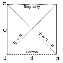
The metric (2) is valid outside the Schwarzschild black hole horizon, , and , where , while the metric (3) covers the Schwarzschild black hole interior , and , where . These two metrics are connected by the analytical continuation
| (4) |
The Carter-Penrose diagram for the interior metric in the coordinates is shown on Figure 1. The lines are null rays propagating within the 2D section . It should be stressed that this diagram is different from the usual Carter-Penrose diagram for the radial sector of the Schwarzschild black hole.
Following Geroch ; Chandrabook we present the metric for the vacuum axisymmetric static distorted black hole in the form
| (5) | |||||
| (6) | |||||
The metric (5), where and are functions of , is valid in the black hole exterior. The metric (6), where and are functions of , describes the interior of the distorted black hole. The black hole horizon is defined by the equation
| (7) |
For a regular black hole the functions and must be smooth and finite at the horizon. In particular, these functions, which define the geometry of the 2D horizon surface, must be continuos across the horizon. The metrics (5) and (6) are regular along the axis of symmetry (no conical singularities), provided
| (8) |
Denote
| (9) | |||||
| (10) |
Then, the vacuum Einstein equations for the metric (6) reduce to the following relations
| (11) | |||||
| (12) | |||||
| (13) |
Here
| (16) |
The functions and obey the relation
| (17) |
Thus, after solving equation (11), one can obtain by simple integration
| (18) |
where the integral is taken along any path connecting and .
The factor is singular along the lines and . Nevertheless, as we shall demonstrate in the next Section, the solutions for for the distorted black holes which are regular at the horizon remain smooth and regular along these lines.
Let us focus on equation (11). Since , a solution to this equation can be presented as a sum of two solutions, one being odd and the other being even function of . Because of the presence of factor in , this operator is singular at , hence, the regular at the horizon solution must be an even function of . This solution remains real after the Wick’s rotation (4).
Studying the exterior solution
| (19) |
Geroch and Hartle Geroch demonstrated that if is a regular smooth function in any small open neighborhood of (including itself) which takes the same values, , on the both ends of the segment ,
| (20) |
then the solution is regular at the horizon and describes a distorted black hole.
The surface gravity of the distorted black hole is
| (21) |
If the distortion source obeys the strong energy condition has to be non-positive Geroch .
Let us emphasize that equation (19) for the ‘gravitational potential’ in the exterior region is elliptic, while the interior equation (11) is of the hyperbolic type. This is in accordance with the general property of black holes. Namely, direction to the singularity in the inner region is the direction to the future, and the evolution of the metric in this region obeys dynamical equations. After solving the equations in the exterior region we obtain boundary conditions at the horizon for the inner dynamical equations. In our particular case the solutions of the exterior and interior problems are connected by the analytical continuation (4).
It is convenient to consider dimensionless form of the metric , connected to the metric as follows
| (22) |
Introducing the quantities
| (23) |
one can write the metric in the form
| (24) | |||||
In what follows, we shall study the metric (24) and its properties. In order to obtain the corresponding characteristics of the ‘physical’ solution (6) it is sufficient to use the scaling transformations (23).
III Interior solution
III.1 Gravitational potential in the inner region
Our goal is to study the interior of a distorted black hole. To find the metric inside the distorted black hole we start with equation (11). This equation allows a separation of variables
| (25) | |||
| (26) |
Since the polar points are regular, the functions must be finite at these points. The solutions of this eigenvalue problem are
| (27) |
Expanding over the complete set of Legendre polynomials of the first kind, , one has
| (28) |
Since at the horizon surface is finite and regular, one must omit infinitely growing at solutions of (26). Thus, we obtain the following solution for
| (29) |
where are the coefficients called multipole moments. For a given value of on the horizon these coefficients are
| (30) |
The condition (20) implies
| (31) |
Since the Legendre polynomials have the symmetry property
| (32) |
the function is invariant under the transformation
| (33) |
that is
| (34) |
This relation implies, in particular, that the value of at the singularity is determined by its values on the horizon
| (35) |
In other words, there exists an interesting duality between the horizon and singularity. It should be emphasized that the functions and , (see (II) - (II)), contain both, symmetric and antisymmetric parts with respect to the reflection (33). This means that the function does not possesses the symmetry (34). Nevertheless, since the function and boundary conditions (8) determine uniquely, the relation (34) simplifies greatly the study of the spacetime structure near the singularity. We return to this point in Section V.
III.2 Boundary values of and
Let us denote
| (36) |
It is easy to check that
| (37) | |||||
| (38) |
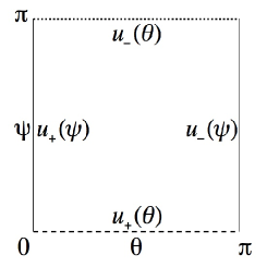
One has (see Figure 2)
| (39) | |||||
| (40) |
We call these data the boundary value of . The regularity of follows from the regularity of the distortion on the horizon and the condition (37).
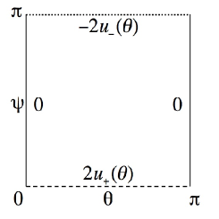
The boundary values of can be obtained from (18). Namely, integrating along the lines , , and , one obtains (see Appendix B)
| (41) |
The boundary values of are summarized on Figure 3.
III.3 Proper time of free fall to the singularity along the symmetry axis
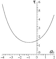
Suppose a function for a distorted black hole is given. Then the boundary data for and described above allow one to calculate, for example, a proper time of a free fall of a test particle from the horizon to the singularity along the symmetry axis. Consider a particle with zero energy and angular momentum which is moving along and . The proper time of its free fall from the horizon to the singularity along the symmetry axis calculated for the metric (24) is given by
| (42) |
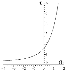
The signs are for and axes, respectively. To illustrate how the distortion of the black hole affects this time we consider two simple cases. As the first example, we consider the quadrupole distortion when only and do not vanish. Taking into account that (see (31)) one has
| (43) |
The integral (42) can be calculated exactly
| (44) |
where is the modified Bessel function. A plot of as a function of the quadrupole moment is shown on Figure 4 (a).
 |
 |
|||
As a second example we consider the octupole distortion when only and do not vanish. Because of (31) one has , and
| (45) |
To obtain we used numerical integration. Plot of as a function of the octupole moment is shown on Figure 4 (b). The minimal value of corresponds to . The similar plot for can be obtained by the reflection .
IV Near horizon geometry
IV.1 Shape of a distorted horizon
The form of the horizon surface for the metric (24) is determined by the following line element (see also Geroch )
| (46) | |||||
This metric is obtained from (24) as the limit of the metric on 2D section of . The horizon area is .
The Gaussian curvature of the metric is , where is the Ricci scalar curvature. It is given by the following expression
| (47) | |||||
where the prime denotes a derivative with respect to .
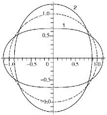
As the special examples, we consider the quadrupole and octupole distortions with functions given by (43) and (45) respectively. The Gaussian curvature for these distortions is
| (48) | |||||
| (49) | |||||
For the quadrupole distortion the Gaussian curvature becomes negative at both of the poles, and , for . Similarly, for the octupole distortion, the Gaussian curvature becomes negative at one of the poles for . It means that for these values of the parameters the horizon surface of the distorted black hole cannot be isometrically embedded in a flat 3D space (see e.g. FR and references therein). For (in the quadrupole case) and (in the octupole case) isometric embeddings are possible.
 |
 |
|||
To construct the embedding we consider a surface
| (50) |
in 3D Euclidean space with the metric
| (51) |
The geometry induced on this surface,
| (52) |
coincides with the horizon surface geometry (46) if
| (53) | |||||
| (54) |
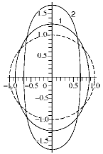
Figure 5 shows the embedding diagrams of the distorted event horizon surface for the quadrupole and octupole distortions.
IV.2 Kretchmann invariant
The function , which specifies the geometry of the horizon surface, uniquely determines the geometry of the black hole interior. In particular, one can obtain expansion of and at the vicinity of the horizon (see Appendix B). The first two terms of this expansion in the powers of are
| (55) | |||||
Here and later we use the dots for the omitted terms of higher order in . We also defined
| (57) |
In this approximation the metric near the black hole horizon reads
| (58) |
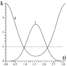
This expansion, for example, can be used to determine the value of the Kretchmann scalar at the horizon surface. Using (IV.2) calculations give
| (60) |
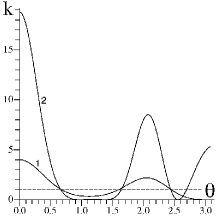
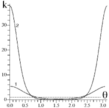
For undistorted Schwarzschild black hole . Figure 6 illustrates the ratio, , of the Kretchmann scalars of the distorted and Schwarzschild black holes.
 |
 |
|||
Comparing this result with (47) one can arrive to the following relation valid on the horizon surface of a distorted black hole
| (61) |
This relation is valid not only for axisymmetric case but also for an arbitrary static distorted black hole (see Appendix A). It is possible to show that the metric of the distorted spherical black holes is of type D both on the horizon and on the axis of azimuthal symmetry, Papa .
V Spacetime near the singularity of a distorted black hole
V.1 Asymptotic form of the metric
Because of the symmetry property (34), the asymptotic form of near the singularity can be easily obtained from its asymptotic expansion near the horizon . After this, the relation (18) allows one to find the expansion of . The expansions for and near the singularity are given in Appendix B. Using these expansions one can obtain the asymptotic form of the metric (24) at
| (62) |
Expressions (V.1) are sufficient to calculate the Kretchmann scalar near the singularity up to the second order in corrections
| (64) | |||||
| (65) |
Higher order terms can be obtained by using the relations given in Appendix B. In the absence of distortion, when , the Kretchmann scalar does not depend on
| (66) |
This is the value of for the Schwarzschild geometry. It can be shown that the metric of a distorted black hole is of type D near the singularity Papa .
V.2 Stretched singularity
For the Schwarzschild geometry the metric near the singularity
| (67) |
can be written in the form
| (68) |
Here is the proper time of a free fall to the singularity along the geodesic . The quantity is negative, and it reaches at the singularity. The metric (68) has the Kasner-like behavior with indices . It describes a metric of collapsing anisotropic universe, that shrinks in - directions, and expands in direction.
The Kretchmann invariant as a function of the proper time has the following asymptotic form
| (69) |
This relation shows that the surface of constant is at the same time a surface of constant .
Spacetime in the region where the curvature is of order of the Planckian curvature requires quantum gravity for its description. For the Schwarzschild geometry at the surface where the proper time is of order of the Planckian time . Since one cannot rely on the classical description in this domain, it is natural to cut the region where the curvature is higher than the Planckian one and to consider its boundary as the stretched or ‘physical singularity’. For the Schwarzschild metric the stretched singularity surface has the topology . Its metric is a direct sum of the metric of a round two-sphere and a line.
What happens to the stretched singularity when the metric of the black hole is distorted? To answer this question we use the asymptotic form of the metric near the singularity, (62). Consider a timelike geodesic lying on the ‘plane’ , . We call such a geodesic ‘radial’. It can be shown (see Appendix C) that a ’radial’ geodesic is uniquely determined by the limiting value of its angular parameter at which it crosses the singularity. Denote by the proper time along the ’radial’ geodesic to its end point at the singularity. In coordinates the metric is given by (68) where is replaced by
| (70) |
We can use as new coordinates in the vicinity of the singularity. Relations (134), (135) connect these ‘new’ coordinates with the ‘old’ ones . The Kretchmann scalar (64), (65) in ‘new’ coordinates reads
| (71) | |||||
| (72) | |||||
The expansion (71) coincides in the leading order with (69). Hence, in the presence of distortion surfaces of equal are again (in the leading order) surfaces of constant .
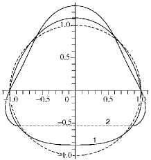
V.3 Shape of equi-curvature surfaces
A surface where the Kretchmann scalar has constant value . In the vicinity of the singularity (in the leading order in ) and on are related as follows
| (73) |
and one has the relation . Consider the induced geometry on . Using this relation one can conclude that term in (62) gives quadratic in corrections only. Neglecting all such terms in (62) we obtain the following expression for the leading asymptotic for the induced metric on
| (74) |
where is given by (70). The surface has the same topology as in the absence of distortion, but its geometry is different. This difference manifests itself in the shape of 2D surfaces. The information about the shape is encoded in the 2D metric . The total area of the surface is . The metric (70) can be obtained from the horizon metric , (46), by a simple change . Under this transformation the even multipole coefficients are invariant, while the odd coefficients change their sign (see (36)). In particular, the embedding diagrams for the metric (70) are the same as shown on Figure 5 (a), with the same value of , and with the opposite value of the octupole moment , as shown on Figure 5 (b).
VI Exact solutions
For any given set of multipole coefficients that determine , the corresponding function can be found explicitly in terms of elementary functions. Since the general expression for is rather cumbersome we do not present it here. Instead, we consider special case of the quadrupole and octupole distortions when the gravitational potential is of the form
| (75) |
where
| (76) |
Substituting this solution into equations (II), (II), and integrating according to equation (18) we derive
| (77) | |||||
where
| (78) | |||||
Exterior metric for a black hole distorted by a quadrupole field was derived in Dor .
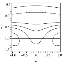
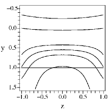
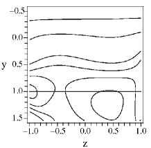
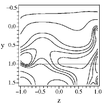
Using GRtensorII package we calculated the Kretchmann scalar for this distortion. We made the calculations for both the inner and external regions. It is easy to check that ’s in these regions are related by the analytical continuation (4). Figures 7 and 8 show the contour lines of for the quadrupole and octupole distortions respectively. In order to plot both the exterior and interior regions simultaneously we introduce new coordinate
The sector , , where , covers the inner region, and the sector , covers the exterior of the black hole.
 |
 |
|||
 |
 |
|||
VII Interior of a caged black hole
In this Section we apply the obtained results to a special case of the so called ‘caged’ black hole. Such a black hole is a solution of the vacuum Einstein equations for a spacetime where one (or more) spatial dimensions are compactified. Caged black holes in 4D spacetime were discussed in FrFr (see also Myers:87 , BoPe:90 ). As the result of the compactification the event horizon of the black hole is distorted. The metric is axisymmetric and is a special case of the Weyl solution. The value of at the horizon found in FrFr [ equation (62)] gives
| (79) |
where and . In this case , is a dimensionless parameter equal to the ratio of the black hole mass, , to the radius of the compactification, , , and
| (80) |
The function has the following properties:
| (81) |
and at the interval it can be approximated by a linear function
| (82) |
with accuracy of 1% . The coefficients for this solution can be obtained from (30). Let us emphasize that since the function is invariant under the transformation , the coefficients for odd vanish (see equations (36), (37)). This implies that and the boundary value of at coincides with the boundary value of this function at the horizon, (see equation (39)), and we have (see equation (20))
| (83) |
 |
 |
|||
From equations (79) and (83) we derive
| (84) |
The metric (46) on the surface of the horizon is
| (85) | |||||
Using equations (60), (61), and (71), (72) we can calculate the Kretchmann scalar at the horizon surface of a caged black hole
| (86) |
and in the vicinity of its ’physical singularity’
| (87) | |||||
| (88) | |||||
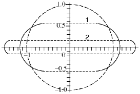
Applying equations (53), (54), and the transformation respectively we can construct embedding of these surfaces. Figure 9 illustrates the shapes of the distorted event horizon surface and the ratio of the Kretchmann scalars , , of the caged and Schwarzschild black holes. The metric (70) on the surface of the stretched singularity is
| (89) | |||||
The shape of distorted ’physical singularity’ is illustrated on Figure 10.
VIII Discussions
Let us summarize the obtained results. We considered the geometry of static vacuum axisymmetric distorted black holes. We focused mainly on the properties of the horizon and interior of such black holes. The geometry of a distorted black hole is uniquely determined by the ’gravitational potential’ which is a solution of the 3D flat Laplace (in the exterior) or d’Alembert (in the interior) equation. After solving this ‘master’ equation, the second function , which enters the metric, can be obtained by a simple integration.
The ’gravitational potential’ can be written as a superposition of the Schwarzschild potential and the distortion potential . The distortion is determined by the values of the multipole coefficients obeying the constraints (31). The distortion potential in the black hole interior possesses a remarkable discrete symmetry (34) which relates the value of in the vicinity of the singularity to its value at the horizon. Thus, the functions , (see (36)), determine both, the shape of the horizon and the leading asymptotics of the metric and curvature invariants near the singularity.
Qualitatively, the shape of the event horizon surface of distorted black hole is similar to the shape of equipotential surfaces in the linearized (Newtonian) gravity. Namely, consider a point-like mass . In the presence of a quadrupole distortion its Newtonian gravitational potential reads (up to constant )
| (90) |
where is the radial distance from the mass , and is the value of the quadrupole moment. For positive such a distortion is generated, for example, by a ring of mass and radius located in the equatorial plane. For such a ring . Similarly, a negative is generated, for example, by two point masses located on the axis of symmetry on the opposite sides of the mass at the distance . In this case . We consider and assume that the distortion is small. Then the change in the position of the equipotential surface for (90) with respect to the position of the unperturbed surface of is
| (91) |
Thus the quadrupole distortion deforms the equipotential surfaces and makes them either oblate (for ), or prolate (for ). This property is similar to the property of the horizon surface for the distorted black hole (see Figure 5 (a)).
It should be emphasized that the linear approximation is not sufficient for the ‘explanation’ of the Kretchmann invariant properties. Really, in the linear approximation
| (92) |
the Kretchmann scalar is
| (93) |
Its variation under the small distortion is
| (94) |
Hence in the weak field approximation, is larger at the points where , such as at the pole of the oblate equipotential surface (for ), and in the equatorial points of the prolate surface (for ). This behavior of in the weak field limit is opposite to the behavior of on the horizon of the distorted black hole (see e.g. (61)). This difference demonstrate that non-linear effects and the spatial curvature are important near the horizon.
The property (61) has an important consequence for caged black holes discussed in Section VII. For close to , when the ‘north’ and ‘south’ poles of the caged black hole are close to one another, the Gaussian curvature (and hence the Kretchmann invariant) becomes large at the poles. In other words, in the infinitely slow merger transition, the region of a very high curvature ’leaks’ through the horizon in the vicinity of the black hole poles. When this curvature reaches the Planckian value, one can say that the ’physical singularity’ (as defined in subsection B of Section V) becomes naked. This may indicate that during the phase transition between black-hole and black-string phases one can expect a formation of a naked ’physical singularity’. Whether this conclusion remains valid for higher dimensional caged black holes and beyond the adiabatic approximation is an interesting open question.
Acknowledgements.
This research was supported by the Natural Sciences and Engineering Research Council of Canada and by the Killam Trust.Appendix A Kretchmann invariant and Gaussian curvature on the horizon of a static black hole
In this appendix we show that the Kretchmann invariant calculated at the horizon of a 4D static distorted black hole is related to the Gaussian curvature of the 2D horizon surface as follows
| (95) |
Let us emphasize that this relation is valid for an arbitrary (not necessarily axisymmetric) distorted black hole. To establish this relation we use the results of paper FrSa .
The metric near the horizon of a static vacuum distorted black hole can be written in the Israel coordinates Israel as follows
| (96) |
where is the square of the timelike Killing vector ,
| (97) |
Here means the covariant derivative with respect to 2D metric , and are the operators associated with this metric. Using the properties of the Killing vector one can show that in the Ricci flat spacetime the following relations are valid
| (98) | |||||
| (99) | |||||
| (100) | |||||
| (101) | |||||
| (102) |
Here is the Gaussian curvature of 2D surface . The Kretchmann invariant for the metric (96) can be written as follows (see equation (4.18) of FrSa )
| (103) |
One can show that quantities , and are finite at the horizon and its vicinity they allow a representation in the form of the Taylor series
| (104) | |||||
| (105) | |||||
| (106) |
Equations (104) imply that the third term in the squared brackets of (103) vanish at the horizon . Simplifying the other two terms by using (105) and (106) one obtains (95).
Appendix B Asymptotic expansions near the horizon and singularity
The solution (29) can be used to find the asymptotic behavior of near the horizon, , and singularity, . To deal with both cases simultaneously, we denote and . The function is an even function of (), and it has the following expansion
| (107) |
Here are functions of angle . The operator in (9) has the same form for both the variables
| (108) |
Using the series expansion for
| (109) | |||
| (110) |
where are the Bernoulli numbers
| (111) |
the relation
| (112) |
and equation (11) one obtains
| (113) | |||||
| (114) | |||||
| (115) | |||||
Appendix C Geodesic motion near the singularity
For a free particle moving in the black hole interior there exist two integrals of motion connected with the spacetime symmetry
| (121) |
The first has the meaning of the conserved momentum along axis, and the second one is the angular momentum.
Consider a point near the singularity of a distorted black hole. What is the proper time required to fall from this point to the singularity? This time depends on the value of and . We consider the proper time for the special value of these parameters . In this case, for a moving particle and . For the Schwarzschild geometry this is the radial motion. We also call the motion in the interior of a disported black hole ‘radial’ when . This type of motion is a geodesic in 2D metric
| (122) |
obtained by dimensional reduction from (62).
Let us denote
| (123) |
Then the Christoffel symbols for the metric are
| (124) | |||
| (125) |
The geodesic equation
| (126) |
in the metric (122) takes the form
| (127) | |||
| (128) |
Here the overdot denotes derivative with respect to the proper time . These equations obey the constraint
| (129) |
that is the normalization condition, , for -velocity.
In the leading order the geodesic equations (127)-(128) and the constraint (129) take the form
| (131) | |||
| (132) | |||
| (133) |
According to (130), the order of approximation in the geodesic equations corresponds to the order of approximation of the metric (62).
We use the ambiguity in the choice of to put at the singularity for each of the ‘radial’ geodesics approaching the singularity. Since grows along geodesics directed to the singularity, it is negative before the geodesic approaches the singularity. The point is a singular point of the equations (131)-(133). To find approximate solution to the geodesic equations one can apply the method of asymptotic splittings described in CotBar . A ‘radial’ geodesic approaching the singularity is uniquely determined by the limiting value . The asymptotic expansion of and near is of the form
| (134) | |||||
| (135) |
where .
References
- (1) W. Israel, Phys. Rev. 164, 1776 (1967).
- (2) V. P. Frolov and N. Sanchez, Phys. Rev. D 33, 1604 (1986).
- (3) W. Israel and K. A. Khan, Nuovo Cimento 33, 331 (1964).
- (4) W. Israel, Lett. Nuovo Cimento 6, 267 (1973).
- (5) L.A. Mysak and G. Szekeres, Can. J. Phys. 44, 617 (1966).
- (6) P. C. Peters, J. Math. Phys. 20, 1481 (1979).
- (7) R. Geroch and J. B. Hartle, J. Math. Phys. 23, 680 (1982).
- (8) S. Chandrasekhar, The Mathematical Theory of Black Holes, Clarendon Press, Oxford, (1983).
- (9) S. Fairhurst and B. Krishnan, Int. J. Mod. Phys. D 10, 691 (2001).
- (10) R. C. Myers, Phys. Rev. D 35, 455 (1987).
- (11) T. Harmark and N. A. Obers, JHEP, 05, 032 (2002).
- (12) A. R. Bogojevic and L. Perivolaropoulos, Mod. Phys. Lett. A 6, 369 (1991).
- (13) A. V. Frolov and V. P. Frolov, Phys. Rev. D 67, 124025 (2003).
- (14) C. W. Misner, K. S. Thorne and J. A. Wheeler, Gravitation, W. H. Freeman and Co., San Francisco, (1973).
- (15) V. P. Frolov, Phys. Rev. D 73, 064021(2006).
- (16) D. Papadopoulos and B. C. Xanthopoulos, Il Nuovo Cim. 83B, 113 (1984).
- (17) A. G. Doroshkevich, Ya. B. Zel’dovich and I. D. Novikov, Zh. Eksp. Teor. Fiz. 49, 170 (1965).
- (18) S. Cotsakis and D. Barrow, gr-qc/0608137.