Ab-initio formulation of the 4-point conductance of interacting electronic systems

Abstract

We derive an expression for the 4-point conductance of a general quantum junction in terms of the density response function. Our formulation allows us to show that the 4-point conductance of an interacting electronic system possessing either a geometrical constriction and/or an opaque barrier becomes identical to the macroscopically measurable 2-point conductance. Within time-dependent density-functional theory the formulation leads to a direct identification of the functional form of the exchange-correlation kernel that is important for the conductance. We demonstrate the practical implementation of our formula for a metal-vacuum-metal interface.

I Introduction

Impressive progress has been achieved within the non-equilibrium Green’s function (NEGF) formulation of quantum transport using the simple ground-state density-functional exchange-correlation potential in a self-consistent formulation Taylor02 ; Basch05 (NEGF-DFT). However, limitations of the latter approximation were recently identified Sai05 ; Jung07 ; Toher05 ; Burke05 ; Palacios05 ; Stefanucci04 ; DiVentra04b ; Koentopp07 . For instance, NEGF-DFT’s omission of the derivative-discontinuity in the exchange-correlation energy functional was found responsible for serious errors in transport calculation through localized resonant levels Toher05 ; Burke05 . Improvements through an (spin-) unrestricted NEGF-DFT formulation have been argued to describe properly some aspects of the Coulomb blockade in quantum junctions Palacios05 . At this level of the theory the exchange-correlation potential of the equilibrium system, $v_{xc}$, is responsible for the electron interaction effects.

In a further theoretical development, Na Sai et al. Sai05 identified a dynamical correction to the resistance of a quantum junction stemming from the contribution of the exchange-correlation electric field to the overall drop in the total potential. They estimated the correction within time-dependent current-density functional theory Vignale97 (TDCDFT) and showed that it has its origin in the non-local density-dependence of the functional. The very applicability of time-dependent density-functional theory (TDDFT) to the problem of quantum transport in the long-time limit has been discussed in depth by Stefanucci and Almbladh Stefanucci04 and by Di Ventra and Todorov DiVentra04b .

Several authors have proposed alternative treatments that avoid the complexities of the exchange-correlation kernels of TD(C)DFT, either by treating the central region with the configuration integration method Delaney04 ; Fagas06 while approximating the non-equilibrium distribution of the electrons, or by using the usual NEGF-DFT approach in combination with a model self-energy within the central region Ferretti05 . More systematic approach to the self-energy can be obtained through well tested approximations like the $GW$ method Darancet07 ; Thygesen07 . Due to the large computational demand so far only very small systems with restricted size of the basis set could be studied. However, the results are encouraging, e.g. the Kondo effect phenomenology seems to be well described within the self-consistent $GW$ method Thygesen07 .

Nonetheless, a systematic approach for addressing the conductance of a fully interacting system at the ab-initio level is not available. This is partly due to the fact that the very formulation of the NEGF formalism Meir92 is based on the concept of noninteracting electrodes and demands partitioning of the system and the electron-electron interaction Prange63 . Stefanucci and Almbladh Stefanucci04 showed that the partitioning can be avoided in principle but practical inclusion of the many-body interactions into the formalism seems to be extremely cumbersome. Fortunately, partitioning is not necessary within the linear response formulation. Several authors have addressed the conductance of interacting system of electrons within the framework of the Kubo formalism arriving at a 2-point Landauer-like formula for the conductance Malet05 ; Prodan07 ; Bokes04 ; Koentopp07 by making certain assumptions about the steady-state total electric field. There is, however, a problem with this derivation since it ignores the charge redistribution in the conducting system when the steady state is forming. In fact, ignoring these aspects one quickly arrives at various unphysical corrections to the conductance Bokes_condmat06 . The problem of charge redistributions has been first pointed out by Thouless Thouless81 . Later Kamenev and Kohn Kamenev01 cast it into a self-consistent framework for many-terminal conductance.

In our work we further develop the formalism that treats the charge redistribution correctly, find its physical interpretation in terms of a time-dependent transient process that leads to the establishment of a current-carrying steady state, and derive a closed formula for the 4-point conductance that is well-defined formally as well as physically.

To describe quantum transport it is necessary to consider the production of a steady state with nonzero current in a generic quantum junction, starting from the ground state (or more generally, from an equilibrium ensemble at finite temperature). Physically, we expect to achieve a steady state that has a uniform average current $I$ flowing through the system, accompanied by a total potential exhibiting a drop $V$ across it. As was advocated many years ago by Landauer Landauer57 , $V$ arises from the resistivity dipole, a local charge imbalance of a piled-up charge in the front and depleted charge behind a quantum junction. Physically such a state is reached by attaching a macroscopic battery to the circuit that pumps electrons from one electrode to the other until a certain potential difference between these two is established. For modeling purposes this mechanism cannot be used directly . Here we will use a construct based on an auxiliary homogeneous vector potential $\vec{A}^{aux}(t)=-\int_{0}^{t}\vec{E}^{aux}(t^{\prime})dt^{\prime}$, pointing in the direction of the eventual flow of current, giving a momentum transfer to all the electrons in the infinite system within a finite interval of time. (This auxiliary vector potential is similar in spirit to the one used by R. Gebauer and R. Car to model a nanojunction using periodic boundary conditions Gebauer04b . There, in contrast to our work, the vector potential grows linearly in time for all $t>0$ and the work exerted on the system must be dissipated via auxiliary phonons located in the electrodes.) The infinite extent of the system is formally essential to our treatment. It is necessary for a continuous spectrum and for giving a momentum transfer at $t=0$ to infinitely many electrons present in the system so that the current will flow for all times $t>0$. However, we would like to mention already at this point that in practical calculations the necessity of the infinite extension can be relaxed so that the formulation can be used for practical ab-initio calculations.

II The non-local conductivity and conductance

The response of the current density to a general external electric field is given within the linear response theory by Kubo59

$$\vec{j}(\vec{r},t)=\int_{-\infty}^{t}dt^{\prime}\int d^{3}r^{\prime}\vec{\vec{\sigma}}(\vec{r},\vec{r}^{\prime};t-t^{\prime})\cdot\vec{E}^{ext}(\vec{r}^{\prime},t^{\prime}).$$ (1)

For simplicity we introduce a symbolic notation for the above equation in the form $\vec{j}=\vec{\vec{\sigma}}\star\vec{E}^{ext}$. In our work, the role of the external field is taken by the auxiliary field $\vec{E}^{aux}$ that is homogeneous and has only a finite duration, i.e. it is absent for large times and it bears no information about the drop in potential in the long-time limit. The latter is contained within the induced field $\vec{E}^{i}(\vec{r},t)$, which appears explicitly when considering the irreducible (or proper) conductivity Pines67 ; GuilianiVignaleBook ,

$$\vec{j}=\vec{\vec{\sigma}}\star\vec{E}^{aux}=\vec{\vec{\sigma}}^{irr}\star(\vec{E}^{aux}+\vec{E}^{i}).$$ (2)

The induced field accounts for the electron-electron interaction at the Hartree level, which is usually referred to as the long-range effects of the Coulomb interaction, whereas the rest of the interactions between electrons, the short range part, is included within the irreducible conductivity. The quantity in which we are primarily interested in is the conductance, defined as $G=I/V$ where $V$ is a voltage drop. For $G$, the detailed spatial and time dependence of the current density and the induced field while the steady current is being established are of no relevance. We define the voltage drop as the overall drop in potential of the induced field $\vec{E}^{i}$ along the current flow (along the $z$ axis) between far left and far right,

$$V=\lim_{t\rightarrow\infty}\int_{-\infty}^{+\infty}dzE_{z}^{i}(\vec{r},t),$$ (3)

which will be indicated by a superscript $4P$ in the associated 4-point conductance, $G^{4P}$. This definition is most suitable

Figure 1: (Color-online) Measurement of the voltage between the macroscopic electrodes, where the current density is zero, gives the two-point conductance $G^{2P}=I/(\Delta\mu/e)$. Measuring the voltage drop inside the simulation box (supercell), where the current density is nonzero, gives the four-point conductance $G^{4P}=I/V$. Increasing the supercell the two quantities approach each other (see Sec. V).

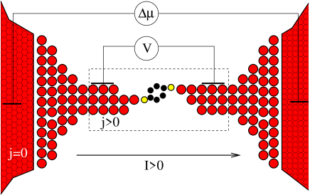
for ab-initio modeling and does not suffer from ambiguities present when one considers two chemical potentials. In mesoscopic physics, the above definition of conductance is referred to as the 4-point conductance (hence the superscript) since it represents measurement of the voltage drop using contacts different from those acting as a source and drain of the current. In the extreme case of a 1D conducting channel of non-interacting, but locally neutral electrons it reduces to the well-known expression $G^{4P}=(2e^{2}/h)(T/R)$. This is in contrast with the most frequently encountered 2-point conductance, $G^{2P}$, where the voltage drop is understood to be the difference in electro-chemical potentials of the two macroscopic electrodes, $\Delta\mu/e$ (see Fig. 1). Since the electrodes are not part of the quantum-mechanical model of the conducting channel, the familiar Landauer result $G^{2P}=(2e^{2}/h)T$ is believed not to be derivable from the Kubo formalism MahanBook and its plausible derivations are always accompanied with steps motivated by physical insight and arguments about phase-incoherent adiabatically widening electrodes Landauer90a . Here we show that for a nanocontact between massive electrodes the 4-point conductance approaches the 2-point Landauer formula. However we never make a reference to $\Delta\mu/e$ and we consistently work with the drop in the induced electrostatic potential only. Our claims for its applicability for the experimental 2-point conductance follow from the fact that for massive electrodes connected with a nanojunction the current density in the electrodes goes to zero and thereby the drop in the induced (Hartree) potential is an excellent indicator of the phenomenological quantity $\Delta\mu/e$. The latter argument serves as a motivation to use the $G^{4P}$ as conceptually and formally well defined quantity to characterize systems of fully interacting electrons in any geometry of the junction.

III Singularity in the response function and the 2-point conductance

An essential property of the conductivity response function of extended systems capable of coherent transport is their singular long range character for large times or – equivalently – as the frequency approaches zero Bokes04 . To show this behavior explicitly we need to introduce a few geometrical details of the studied nanojunction which do not restrict the generality of our argument. We consider a geometry where $z$ is a direction of the current flow, $q$ a reciprocal vector in that direction, and for clarity we assume that the system can be put into a periodic supercell along the $x,y$ directions. The conductance $G^{4P}$ is then a conductance for the area of the supercell $S$. To find the current flowing through $S$, we integrate Eq. (2) across the cross-sectional area. This naturally leads to the cross-section integrated conductivity Sols91

$$\sigma^{irr}(z,z^{\prime};t)=\int_{S}\int_{S}d\vec{S}\cdot\vec{\vec{\sigma}}^{irr}(\vec{r},\vec{r}^{\prime};t)\cdot d\vec{S}^{\prime},$$ (4)

which relates the current to the $z$-component of the total field,

$$I(z,t)=\int^{t}dt^{\prime}\int_{-\infty}^{\infty}dz^{\prime}\sigma^{irr}(z,z^{\prime};t-t^{\prime})(E^{aux}(t^{\prime})+E^{i}(z^{\prime},t^{\prime})).$$ (5)

The singular long-range character appears as the independence of $\sigma^{irr}(z,z^{\prime};t)$ on $z$ and $z^{\prime}$ as $t\rightarrow\infty$ which when performing the Fourier transforms $z,z^{\prime}\rightarrow q,q^{\prime}$ and $t\rightarrow\omega+i\alpha$, takes the form Bokes04

$$\lim_{\omega\rightarrow 0}\sigma^{irr}(q,q^{\prime},\omega+i\alpha)=2\pi G^{2P}\delta(q)\delta(q^{\prime}),$$ (6)

where we have formally introduced the 2-point conductance, $G^{2P}$, as the strength of the above mentioned singular character. To extract the strength we introduce a linear functional $\mathcal{G}^{\sigma}[]$

$$\mathcal{G}^{\sigma}[\sigma^{irr}]=\lim_{\alpha\rightarrow 0^{+}}\int\int\frac{dqdq^{\prime}}{2\pi}\sigma^{irr}(q,q^{\prime};i\alpha),$$ (7)

for which we simply have $G^{2P}=\mathcal{G}^{\sigma}[\sigma^{irr}]$. It has been shown previously that this identification is correct for noninteracting electrons Bokes04 . Further motivation to refer to it as a 2-point conductance for interacting systems will be discussed in Section V.

IV Onset of the current inside the electrodes

The Eq. (5) can now be analyzed in the light of the above observations. First, let us consider a distant part of one of the electrodes, $|z|\gg 0$, for times such that $1/E_{F}\ll t\ll|z|/v_{F}$, where $E_{F}$ and $v_{F}$ are the Fermi energy and Fermi speed respectively. In this regime, the response in the electrodes ($|z|\gg 0$) is determined by the electrode itself, independently of the nanojunction. After a short relaxation time ($\sim 1/E_{F}$) the auxiliary field establishes a uniform (i.e. $z$-independent) current inside the electrode

$$I(z,t)=\int dz^{\prime}\int_{-\infty}^{t}dt^{\prime}\sigma^{irr,e}(z,z^{\prime};t-t^{\prime})E^{aux}(t^{\prime}),$$ (8)

where $\sigma^{irr,e}$ is the irreducible conductivity of the electrode only while preserving the local charge neutrality within the electrode. We are free to choose any time-dependence of the field as long as it delivers finite change of momentum for each electron and thus establishes the eventual steady current; the most convenient choice is $E^{aux}(t)=-A^{aux}\delta(t)$, where $A^{aux}$ is the magnitude of the change in the homogeneous vector potential at $t=0$.

This picture is not valid as one approaches the region of the nanojunction, i.e. for $z\sim 0$. Still, since the current will keep coming from the left electrode and disappearing into the right electrode (there is always such $|z|\gg 0$ that for any time $t$ we have $t\ll|z|/v_{F}$ and hence the above analysis can be applied), the charge will have to pile up in front of the junction and similarly deplete behind the junction, creating a resistivity dipole Landauer57 . The incoming current cannot be decreased by some form of reflected front/disturbance from the junction since this would break the local charge neutrality within the electrode, leading to strong opposing fields. Hence the dipole around the junction and therefore the drop in the induced potential $V$ will grow, increasing the current in the junction region until it becomes equal to the current, $I$, deep inside the electrode, as described in the preceding paragraph. This will be possible since in the linear regime we expect $I=G^{4P}V$.

Having in mind this physical process, the established uniform current at long times expressed by Eq. (8) for the distant electrode applies at all positions including $z=0$. We express the electrode conductivity $\sigma^{irr,e}$ in reciprocal space for long times as

$$I(t\rightarrow\infty) = -\lim_{\alpha\rightarrow 0^{+}}\int dq\sigma^{irr,e}(q,q^{\prime}=0;i\alpha)A^{aux}$$ (9)

$$= \mathcal{F}^{\sigma}[\sigma^{irr,e}]A^{aux},$$ (10)

where we use a small imaginary frequency $i\alpha$ to perform the long-time limit Kubo59 . The linear functional $\mathcal{F}^{\sigma}[]$ will be further discussed in Section VII.

V The 4-point formulation of the conductance

The above physical picture can be directly used within Eq. (5). We write the conductivity of the whole system as the conductivity of an infinitely long electrode alone, $\sigma^{irr,e}$, plus a further term, $\sigma^{irr,j}$, characterizing the presence of the junction: $\sigma^{irr}=\sigma^{irr,e}+\sigma^{irr,j}$. Eq. (5) is thereby cast into the form

$$I = \sigma^{irr,e}\star E^{aux}+\sigma^{irr,j}\star E^{aux}+\sigma^{irr}\star E^{i}.$$ (11)

Evaluating this equation at $z=0$ and using the definitions of the functionals $\mathcal{F}^{\sigma}$ and $\mathcal{G}^{\sigma}$, the equation (11) can be written as

$$I = \mathcal{F}^{\sigma}[\sigma^{irr,e}]A^{aux}+\mathcal{F}^{\sigma}[\sigma^{irr,j}]A^{aux}+\mathcal{G}^{\sigma}[\sigma^{irr}]V.$$ (12)

From Eq. (8) we know that in the long-time limit, the first term on the RHS is itself equal to $I$, so that the second and third terms sum to zero, from which we easily arrive at the central result of this paper

$$G^{4P}=\frac{\mathcal{F}^{\sigma}[\sigma^{irr,e}]}{\mathcal{F}^{\sigma}[\sigma^{irr,e}]-\mathcal{F}^{\sigma}[\sigma^{irr}]}\times\mathcal{G}^{\sigma}[\sigma^{irr}],$$ (13)

where we have used the fact that $\mathcal{F}^{\sigma}[\sigma^{irr,j}]=\mathcal{F}^{\sigma}[\sigma^{irr}]-\mathcal{F}^{\sigma}[\sigma^{irr,e}]$ and that $V=\int dzE^{i}(z)=E^{i}(q=0)$.

It is very instructive to apply the above result for a simple 1D non-interacting gas with a single scattering center. For this system, the noninteracting conductivity in the small frequency limit has a form Kamenev01

$$\sigma^{0}(q,q^{\prime};i\alpha) = \frac{2}{\pi}\frac{v_{F}\alpha}{v_{F}^{2}q^{2}+\alpha^{2}}\delta(q-q^{\prime})$$ (14)

$$-R\frac{2}{\pi}\frac{v_{F}\alpha}{v_{F}^{2}q^{2}+\alpha^{2}}\frac{2}{\pi}\frac{v_{F}\alpha}{v_{F}^{2}(q^{\prime})^{2}+\alpha^{2}}$$

The irreducible conductivity of the homogeneous 1D gas, corresponding here to the electrode in the general case is simply the first part of the above expression

$$\sigma^{0,e}(q,q^{\prime};i\alpha)=\frac{2}{\pi}\frac{v_{F}\alpha}{v_{F}^{2}q^{2}+\alpha^{2}}\delta(q-q^{\prime}).$$ (15)

It is straightforward to see that using the above forms we have $\mathcal{G}^{\sigma}[\sigma^{0}]=(1-R)/\pi=T/\pi$, $\mathcal{F}^{\sigma}[\sigma^{0,e}]\sim v_{F}/\pi\alpha$ and $\mathcal{F}^{\sigma}[\sigma^{0,j}]\sim Rv_{F}/\pi\alpha$, and we arrive at the 4-point conductance $G^{4P}=(1/\pi)(T/R)$. The arguments of local charge neutrality in the electrodes and its consequences are very closely related to the original comment by Thouless Thouless81 and a more recent work by Kamenev and Kohn Kamenev01 . In the form presented in Eq. (13) it is valid for nanojunctions of any shape as long as we can put them into a supercell, including the extreme case of a planar metal-vacuum-metal junction for which we will demonstrate its applicability in Section VII.

The generality of Eq. (13) can be used to show the equivalence of the 2-point and 4-point conductances for nanojunctions with massive electrodes. The demonstration is based on the observation that for such a geometry $\mathcal{F}^{\sigma}[\sigma^{irr,e}]\gg\mathcal{F}^{\sigma}[\sigma^{irr}]$ and hence the prefactor containing the $\mathcal{F}[]$s in Eq. (13) goes to 1. The mentioned inequality is immediately clear from the following argument: $\mathcal{F}^{\sigma}[\sigma^{irr,e}]$ gives the current flowing in the electrodes when the vector potential is changed from zero to $A^{aux}$, whereas $\mathcal{F}^{\sigma}[\sigma^{irr}]$ formally gives current as a response to the same disturbance but in a fictitious system having the same geometry as the real nanojunction but for which the long-range Coulomb interaction is missing. This implies that the local charge neutrality is not enforced (since only the irreducible response enters $\mathcal{F}^{\sigma}$) and as a result most of the electrons coming from one electrode will be reflected from the nanojunction and decrease the current. Hence the resulting current will be much smaller in this second case and the inequality is fulfilled. This formally justifies Landauer’s arguments in favor of the expression $G=T/\pi$ as the conductance of a nanojunction between two phase-randomizing and adiabatically widening reservoirs. As we can clearly see, it is only the widening that is really needed to have the conductance of the junction as a whole be given by Eq. (7). This explains our motivation to refer to the latter quantity as a 2-point conductance even for interacting electronic systems. The argument applies also to opaque barriers, not necessarily having a constriction, which has been explored in previous works Mera05 ; Carva04 and is also demonstrated in Section VII.

VI Inclusion of exchange and correlation into conductance

Having established the validity and generality of Eq. (13) we can proceed to approximations that go beyond non-interacting or Hartree-like interacting electrons. The simplest way to do so is within the framework of time-dependent density-functional theory. Some doubt about the applicability of the latter might arise from the dynamics deep in the electrode described in Section IV. There, the induced current is dominated by a divergenceless component that cannot be related to a time-dependent density, which is the only physically relevant quantity within the TDDFT. However, at the level of Fermi-liquid theory, this divergenceless current is identical to that of a non-interacting system due to the backflow of quasiparticles NozieresBook . Hence for this part we do not expect corrections arising from the exchange and correlation and we should expect $\mathcal{F}^{\sigma}[\sigma^{irr,e}]=\mathcal{F}^{\sigma}[\sigma^{0,e}]$, where $\sigma^{0,e}$ is the non-interacting conductivity of the electrode. On the other hand, the response described by the rest of Eq. (11), leading to the voltage drop in the induced potential, is essentially localized around the nanojunction and is completely described by the time- and space- dependence of the electronic density which is amenable to the TDDFT approach.

To cast our theory into the TDDFT framework, we need to reformulate the functionals $\mathcal{F}^{\sigma}$ and $\mathcal{G}^{\sigma}$ since the conductivity is not directly accessible within TDDFT. The irreducible conductivity is simply related to the irreducible polarization Bokes04 ; Pines67

$$\sigma^{irr}(q,q^{\prime},i\alpha)=-\frac{\alpha}{qq^{\prime}}\chi^{irr}(q,q^{\prime};i\alpha),$$ (16)

which is conveniently calculated via the density response function calculation within TDDFT. To incorporate this we also introduce new functionals of the irreducible polarization

$$\mathcal{F}[\chi^{irr}] = \mathcal{F}^{\sigma}[-\frac{\alpha}{qq^{\prime}}\chi^{irr}(q,q^{\prime};i\alpha)],$$ (17)

$$\mathcal{G}[\chi^{irr}] = \mathcal{G}^{\sigma}[-\frac{\alpha}{qq^{\prime}}\chi^{irr}(q,q^{\prime};i\alpha)].$$ (18)

for which we give explicit expressions suitable for direct numerical evaluation in reciprocal and real space representation in the Appendix. The irreducible polarization satisfies the Dyson equation

$$\chi^{irr}(q,q^{\prime};i\alpha)=\chi^{0}(q,q^{\prime};i\alpha)+$$

$$\int dq^{\prime\prime}dq^{\prime\prime\prime}\chi^{0}(q,q^{\prime\prime};i\alpha)f_{xc}(q^{\prime\prime},q^{\prime\prime\prime};i\alpha)\chi^{irr}(q^{\prime\prime\prime},q^{\prime};i\alpha),$$ (19)

where $\chi^{0}(q,q^{\prime};i\alpha)$ is the non-interacting Kohn-Sham density response function, and $f_{xc}(q^{\prime\prime},q^{\prime\prime\prime};i\alpha)$ is a non-local frequency-dependent exchange-correlation kernel Vignale96 . The above two equations give the 4-point conductance of an interacting electronic system: for a given kernel $f_{xc}$ one needs to invert the Dyson equation (19), substitute the result into Eq. (16) and employ the general expression Eq. (13).

However, we can gain more insight by multiplying Eq. (19) by $-\alpha/(qq^{\prime})$ and taking the limit $\alpha\rightarrow 0$. Clearly, the resulting left-hand-side is singular in $q$, with the strength being $G^{2P}$ according to Eq. (6). The strength of the first term on the right-hand-side of (19) multiplied by the same factor gives the 2-point conductance of the non-interacting Kohn-Sham system, $G^{2P,0}$. The difference between these the two, i.e. the correction due to the exchange-correlation kernel, is then nonzero only if the last term in Eq. (19) also leads to a singular form. This observation can be used to deduce the forms of the kernel that do influence the conductance, since the general character of $\chi$ for small $\alpha$ is well known. The most interesting choice, making use of the character of $\chi^{0/ir}\sim qq^{\prime}$, is $f_{xc}(q,q^{\prime};i\alpha)=\frac{\alpha}{qq^{\prime}}A(q,q^{\prime};i\alpha)$ where $A$ is well-behaved: $A(q,q^{\prime};i\alpha)\rightarrow R^{\tt dyn}=A(q=0,q^{\prime}=0)\neq 0$ for $\alpha\rightarrow 0$. The resulting 4-point conductance then takes the form

$$G^{4P} = \frac{\mathcal{F}[\chi^{0,h}]}{(1+\mathcal{G}[\chi^{0}]R^{\tt dyn})\mathcal{F}[\chi^{0,h}]-\mathcal{F}[\chi^{0}]}\mathcal{G}[\chi^{0}].$$ (20)

In the case of a narrow junction between massive electrodes and using the arguments leading to Eq. (13), we obtain

$$G^{4P}\approx\frac{\mathcal{G}[\chi^{0}]}{1+\mathcal{G}[\chi^{0}]R^{\tt dyn}}=\frac{G^{0}}{1+R^{\tt dyn}G^{0}}.$$ (21)

i.e. in this very important case $R^{\tt dyn}$ represents part of the dynamical resistance, having origin in exchange-correlation effects and can be accounted for by adding this resistance in series with the Kohn-Sham result.

An approximate correction of this form has, in fact, been identified by Na Sai et al. Sai05 for interacting electronic systems with weakly inhomogeneous potential along the direction of the current flow. For such systems it is possible to show that a purely longitudinal exchange-correlation electric field used in their treatment within TDCDFT Vignale96 ; Vignale97 is equivalent to a contribution to the TDDFT kernel of the asymptotic form for small $q,q^{\prime}$

$$f^{(\eta)}_{xc}(q,q^{\prime};\omega)\approx-\frac{i\omega}{qq^{\prime}}A\int dz\frac{4\eta}{3}\left(\frac{\partial_{z}n(z)}{n(z)^{2}}\right)^{2}=-\frac{i\omega}{qq^{\prime}}A^{2}R^{\tt dyn}$$ (22)

where $A$ is the cross-sectional area of the considered system, $n(z)$ is the electronic density and $\eta$ is the dynamical viscosity of a homogeneous electron gas Vignale97 . We should note that for homogeneous systems $R^{\tt dyn}=0$ since $\partial_{z}n(z)=0$. This is important since the functional form $f_{xc}^{(\eta)}$ given above and the limiting process would not lead to a finite result for a homogeneous system. It is interesting to note that the nonlocal character of the kernel, i.e. $f^{xc}\sim 1/q^{2}$ has been found also responsible for significant improvement in the ab-initio studies of the optical spectra in many materials Botti05 ; Reining02 .

A very popular approximation for the exchange-correlation kernel is the adiabatic local-density approximation (ALDA) Gross85

$$f_{xc}^{(ALDA)}(\mathbf{r},\mathbf{r}^{\prime})=f_{xc}^{ALDA}[n^{0}(\mathbf{r})]\delta(\mathbf{r}-\mathbf{r}^{\prime})$$ (23)

$$f_{xc}^{ALDA}[n^{0}]=d^{2}(n^{0}\epsilon_{xc}(n^{0}))/dn^{2},$$ (24)

(Here $\epsilon_{xc}(n^{0})$ is the exchange-correlation energy per particle of a homogeneous electron gas (HEG) of density $n^{0}$), leading to a kernel in the reciprocal space of the form $f_{xc}^{(ALDA)}(q,q^{\prime};\omega)=f_{xc}^{(ALDA)}(q-q^{\prime};\omega)\rightarrow B(\omega)\delta(q-q^{\prime}),B(\omega)\rightarrow B\neq 0$ for $\omega\rightarrow 0$. It has been argued by several authors that ALDA should not contribute to any change in the conductance. Sai05 ; Burke05 The basis of this argument comes from the fact that one can account for the exchange and correlation effects either via the exchange correlation kernel, or by using the exchange-correlation electric field. The latter can be shown to contribute to the conductance only if there is a nonzero drop of the exchange-correlation potential across the system, which is absent within any local or semi-local approximations. The argument is valid also within our theory when applied to Eq. (11). However, it is interesting to explore the consequences if one stays within the kernel-based treatment. Here the proper definition of the 4-point conductance is essential. If one directly uses the 2-point formula in Eq. (7) for metal-vacuum-metal interfaces, one finds nontrivial ALDA corrections solely due to the fact that the Kohn-Sham conductivity does redistribute the charge at long distances when a localized Kohn-Sham potential with nonzero drop is applied Bokes_condmat06 . The numerical results for metal-vacuum-metal presented in Section VII show a cancellation between these ALDA corrections within $\mathcal{G}[\chi^{irr}]$ and those entering $\mathcal{F}[\chi^{irr}]$ within the precision of the numerics so that the $G^{4P}$ coming from Eq. (13) remains unaffected by the ALDA kernel, as it should be. It is important to emphasize this point because studies of exchange and correlation effects using the 2-point formula only for 1D atomic chains Prodan07 or quantum wires Malet05 may easily lead to incorrect conclusions.

VII Conductance of a metal-vacuum-metal interface

The metal-vacuum-metal junction is one of the simplest systems for ab-initio study of electronic transport and hence it conveniently serves as a demonstration that the formula (13) can be numerically implemented even for realistic systems. In practical implementations we cannot work with an infinite system, for which the response function that enters the functionals $\mathcal{F}[~{}]$ and $\mathcal{G}[~{}]$ is needed. Instead, we take a finite system with $z\in(-L,L)$ with zero boundary conditions at the end points. This brings certain restriction on the zero-frequency extrapolation that we will discuss below. The two perpendicular directions can be dealt with easily in the reciprocal space for this particular system.

In our calculations we employ two jellium slabs of thickness $l$ and density given by $r_{s}=3.0$ a.u., separated by a distance $d$, i.e. $2l+d<2L$ where the supercell extends from $-L$ to $L$. The calculation of $\chi^{0}(z,z^{\prime};i\alpha)$ is performed at the self-consistent LDA level Jung04 . Subsequently for the ALDA calculation we invert the Dyson equation, Eq. (4), in real space and thereby calculate the irreducible response $\chi^{irr}(z,z^{\prime};i\alpha)$. The inclusion of the non-local kernel, such as that arising from the viscosity of the electron liquid, can be done directly via Eq. (20), avoiding the inversion of the Dyson equation. For the evaluation of $\mathcal{F}[~{}]$ and $\mathcal{G}[~{}]$ we employ their real space form (Appendix), integrating over the simulation cell,

$$\mathcal{G}_{\alpha}[\chi^{irr}] = \alpha\int_{-L}^{0}\int_{0}^{L}dzdz^{\prime}\chi^{irr}(z,z^{\prime};i\alpha),$$ (25)

$$\mathcal{F}_{\alpha}[\chi^{irr}] = \alpha\int_{-L}^{0}dz\int_{-L}^{L}dz^{\prime}\chi^{irr}(z,z^{\prime})z^{\prime},$$ (26)

keeping $\alpha$ finite for the moment. For extrapolation we need to use imaginary frequencies $\alpha\ll E_{F}$ so that the transient dynamics is removed from the response function. On the other hand, the finite extent of the electrodes restricts the limiting procedure for $\alpha\rightarrow 0$; one can go down no more than to imaginary frequencies $\alpha_{min}\approx v_{F}/l$ ($v_{F}\approx 0.64$ a.u. for $r_{s}=3$ a.u.).

To demonstrate the precision and scaling of our calculation we first present calculations for a non-selfconsistent square-barrier potential (width $8$ a.u., height $0.25$ a.u.) between two 3D electrodes ($E_{F}=0.2$ a.u.). The chosen values are reasonably close to our self-consistent potential but at the same time allow for comparison of with the exact value of $G^{2P}=\lim_{\alpha\rightarrow 0}\mathcal{G}_{\alpha}[\chi^{0}]$ using the analytically known form of the transmission probability. The calculated values of $\mathcal{G}_{\alpha}[\chi^{0}]$ shown in the Fig. 2 for finite slabs and finite frequencies clearly show finite size effects below $\alpha_{min}$.

Figure 2: (Color-online) Dependence of $G^{2P}(\alpha)=\mathcal{G}_{\alpha}[\chi^{0}]$ on frequency $\alpha$ for several electrode widths $l$ (vacuum is fixed for $d=8$ a.u.). For frequencies below the thick line, given by $\alpha_{min}(l)=v_{F}/l$, the finite size effects appear, so that $\alpha\sim 0.05$ are used for extrapolation to zero. The vertical shifts of the individual curves is caused by the oscillation of the Fermi energy (see also Fig. 3).

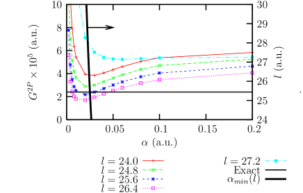
However, even for frequencies larger than $\alpha_{min}$ we observe a remanent horizontal oscillatory dependence of the conductance curves on the electrodes’ width.

Figure 3: (Color-online) Dependence of the extrapolated $G^{2P}$ on the electrodes’ widths $l$ for $d=8.0$ a.u for a square-barrier potential. The inset shows the oscillations in the Fermi energy and the conductance $G^{2P}$ in a restricted range of $l$ for a self-consistent calculation. Choosing widths for which the Fermi energy attains its minima (indicated with dots) leads to a stable estimate of the conductance of the infinite system.

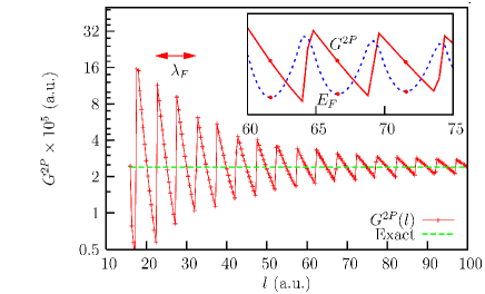
Even though the amplitude of the oscillations for smaller widths are substantial, the overall convergence to the exact value is evident. The oscillatory character of the Fermi energy can be effectively used for identifying the most suitable system widths for an optimal estimate of the infinite system conductance. One should choose the widths for which the Fermi energy attains local minima (inset in Fig. 3), which is the method we use within our work.

Similar extrapolation to zero frequency can be done for $\mathcal{F}[~{}]$, or even better for $\alpha\times\mathcal{F}[~{}]$ which approaches a constant value for an infinite system. However, since our aim is to calculate the 4-point conductances, we directly extrapolate the expression (20) which behaves very similarly as the $G^{2P}(\alpha)$ described in detail in the preceding paragraph.

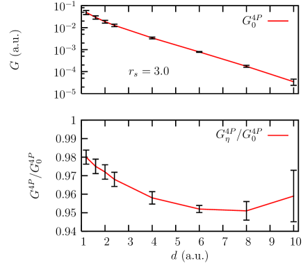
We now apply our methodology to a fully self-consistent calculation for a sequence of vacuum widths $d=1,\ldots,10$ a.u. to study the effect of the recently suggested viscosity-related exchange-correlation correction due to Na Sai et al. Sai05 , and to explore the cancellation of ALDA corrections between $\mathcal{F}[~{}]$ and $\mathcal{G}[~{}]$. The overall dependence of the conductance on $d$ is exponential. For clarity of presentation we show first the exponentially decreasing form of the calculated Kohn-Sham conductance, $G_{0}^{4P}$, in the upper panel of Fig. 4; the small symbols indicate error bars in $G_{0}^{4P}$ due to uncertainty in the extrapolation to zero frequency. For this system the absolute values of the corrected conductances after inclusion of either TDDFT kernel – ALDA kernel or viscosity kernel – lie within these indicated error bars. As we have discussed in Section VI, the ALDA does not lead to any correction, but numerically this result is not trivial. In fact both, the $\mathcal{G}[\chi^{ALDA}]$ and $\mathcal{F}[\chi^{ALDA}]$ do change due to the presence of the exchange-correlation kernel (24), but these changes are canceled in the total expression for the 4-point conductance (13) within the numerical precision of the extrapolation to zero frequency. On the other hand, the corrections due to the finite viscosity of the electron liquid do lead to a small but systematic decrease in the conductance, which is about 5% in the examined range of relative conductances Sai05 ; Jung07 . While this is smaller than the error bar of the extrapolated conductance, since the viscosity correction itself does not involve extrapolation (Eq. 24), the resulting error bar of the relative correction, shown in the lower panel of Fig. 4, is noticeably smaller than the correction itself, and thus the correction is significant.

Figure 4: (Color-online) The Kohn-Sham conductance $G_{0}^{4P}$ with error bars resulting from uncertainty in the extrapolation to zero frequency (upper panel) and the viscosity-corrected conductance $G_{\eta}^{4P}$ (shown relative to $G_{0}^{4P}$) (lower panel), as a function of the vacuum width $d$. Only the corrections due to the non-local kernel lead to changes in the conductance. The ALDA kernel does not affect the Kohn-Sham result within numerical error.

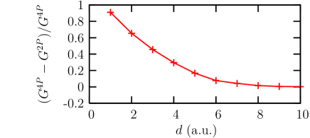
Finally we numerically demonstrate the appropriateness of the 2-point conductance, $G^{2P}=\mathcal{G}[\chi]$ for opaque barriers. The graph in Fig. 5 clearly shows that for $d>4$ the $\mathcal{F}[~{}]$-dependent prefactor is very close to 1, which supports our arguments in Sec. V as well as is in agreement with previous numerical work Mera05

Figure 5: (Color-online) The relative difference between the 4-point and 2-point Kohn-Sham conductances. The difference between the two diminishes for opaque barriers.

VIII Conclusion

In conclusion, we have presented a unified formalism, based on singular character of response functions, that gives the conductance of a general system of interacting electrons. We have derived a closed formula for the 4-point conductance in terms of the many-body response functions: the irreducible conductivity or the irreducible density response. The formulation allows for clear demonstration of the validity of the Landauer formula for broadening or opaque nanojunctions. Furthermore, we have utilized our formulation for examining the exchange and correlation effects on the conductance within the time-dependent density functional theory. We have shown that the long time limit determines the functional form of the exchange-correlation kernel that can lead to nonzero corrections. The exposed theory can be also used for ab-initio calculations for which the achievable precision in conductance calculation for a given size of a finite-size simulation cell has been demonstrated on a simple metal-vacuum-metal junction.

IX Appendix: Evaluation of functionals $\mathcal{F}$ and $\mathcal{G}$.

The functionals $\mathcal{F}[~{}]$ and $\mathcal{G}[~{}]$ were given explicitly in the Fourier-transformed form in Eqs. (9), (10) and Eq. (7) respectively. In numerical calculations it is more advantageous and numerically stable to use their representation in real space. To achieve this, we use the inverse transform of the irreducible density response function defined by

$$\chi(q,q^{\prime})=\int\frac{dzdz^{\prime}}{2\pi}e^{-iqz}\chi(z,z^{\prime})e^{iq^{\prime}z^{\prime}}.$$ (27)

Several times we will have to resolve the integral of the type

$$f(z_{0})=\int\frac{dq}{q}e^{iqz_{0}}\chi(q,q^{\prime}).$$ (28)

Since $\chi(q,.)\sim q$ for small $q$, the integral is well defined and we can choose to interpret the apparent singularity $1/q$ as $1/(q+i\delta)$ or $1/(q-i\delta)$ with $\delta\rightarrow 0^{+}$. Taking the former (the final result is independent of this choice) and using the inverse transform (27) we find

$$f(z_{0})=-i\int dzdz^{\prime}\theta(z_{0}-z)\chi(z,z^{\prime})e^{iq^{\prime}z^{\prime}},$$ (29)

where $\theta(z)$ is the unit step function.

Using the definition of $\mathcal{G}[~{}]$ and using the integral (29) twice with $z_{0}=0$ we readily obtain

$$\mathcal{G}[\chi]=\lim_{\alpha\rightarrow 0^{+}}\alpha\int_{-\infty}^{0}dz\int_{0}^{\infty}dz^{\prime}\chi(z,z^{\prime};i\alpha).$$ (30)

The real-space form of the $\mathcal{F}$ is obtained using again the Fourier transform:

$$\mathcal{F}[\chi] = \left.\alpha\int\frac{dq}{qq^{\prime}}\int\frac{dzdz^{\prime}}{2\pi}e^{-iqz}\chi(z,z^{\prime})e^{iq^{\prime}z^{\prime}}\right|_{q^{\prime}=0}$$ (31)

$$= \left.-i\alpha\int_{0}^{\infty}dz\int_{-\infty}^{\infty}dz^{\prime}\chi(z,z^{\prime})\frac{e^{iq^{\prime}z^{\prime}}}{q^{\prime}}\right|_{q^{\prime}=0}$$ (32)

$$= \alpha\int_{-\infty}^{0}dz\int_{-\infty}^{\infty}dz^{\prime}\chi(z,z^{\prime})z^{\prime}$$ (33)

since we can Taylor expand $e^{-iq^{\prime}z^{\prime}}$ with the linear term giving the only nonzero contribution.

References

- (1) J. Taylor, M. M. Brandbyge, and K. Stokbro, Phys. Rev. Lett. 89, 138301 (2002).
- (2) H. Basch, R. Cohen, and M. A. Ratner, Nano Lett. 5, 1668 (2005).
- (3) N. Sai, M. Zwolak, G. Vignale, and M. DiVentra, Phys. Rev. Lett. 94, 186810 (2005).
- (4) J. Jung, P. Bokes, and R. W. Godby, Phys. Rev. Lett. 98, 259701 (2007).
- (5) C. Toher, A. Filippetti, S. Sanvito, and K. Burke, Phys. Rev. Lett. 95, 146402 (2005).
- (6) M. Koentopp, K. Burke, and F. Evers, Phys. Rev. B 73, 121403(R) (2006).
- (7) J. J. Palacios, Phys. Rev. B 72, 125424 (2005).
- (8) G. Stefanucci and C. O. Almbladh, Phys. Rev. B 69, 195318 (2004).
- (9) M. DiVentra and T. N. Todorov, J. Phys.: Condens. Matter 16, 8025 (2004).
- (10) M. Koentopp, C. Chang, K. Burke, and R. Car, cond-mat/0703591v1 (2007).
- (11) G. Vignale, C. A. Ullrich, and S. Conti, Phys. Rev. Lett. 79, 4878 (1997).
- (12) P. Delaney and J. C. Greer, Phys. Rev. Lett. 93, 036805 (2004).
- (13) G. Fagas, P. Delaney, and J. C. Greer, Phys. Rev. B 73, 241314(R) (2006).
- (14) A. Ferretti, A. Calzolari, R. DiFelice, F. Manghi, M. J. Caldas, M. B. Nardelli, and E. Molinari, Phys. Rev. Lett. 94, 116802 (2005).
- (15) P. Darancet, A. Ferretti, D. Mayou, and V. Olevano, Phys. Rev. B 75, 075102 (2007).
- (16) K. Thygesen and A. Rubio, J. Chem. Phys. 126, 091101 (2007).
- (17) Y. Meir and N. S. Wingreen, Phys. Rev. Lett. 68, 2512 (1992).
- (18) R. E. Prange, Phys. Rev. 131, 1083 (1963).
- (19) F. Malet, M. Pi, M. Barranco, and E. Lipparini, Phys. Rev. B 72, 205326 (2005).
- (20) E. Prodan and R. Car, cond-mat/0702192 (2007).
- (21) P. Bokes and R. W. Godby, Phys. Rev. B 69, 245420 (2004).
- (22) P. Bokes, J. Jung, and R. W. Godby, cond-mat/0604317 (2006).
- (23) D. J. Thouless, Phys. Rev. Lett. 47, 972 (1981).
- (24) A. Kamenev and W. Kohn, Phys. Rev. B 63, 155304 (2001).
- (25) R. Landauer, Z. Phys. B: Condens. Matter 68, 217 (1987).
- (26) R. Gebauer and R. Car, Phys. Rev. Lett. 93, 160404 (2004).
- (27) R. Kubo, in Lectures in Theoretical Physics, Vol. 1, edited by W. E.cBrittin and L. G. Dunham (Interscience, New York, 1959).
- (28) D. Pines and P. Nozieres, The Theory of Quantum Liquids (W. A. Benjamin, Inc., New York, 1966).
- (29) G. F. Giuliani and G. Vignale, Quantum Theory of the Electron Liquid (Cambridge University Press, Cambridge, 2005).
- (30) G. Mahan, Many-Particle Physics (Kluwer Academic/Plenum Publishers, New York, 2000).
- (31) R. Landauer, in Analogies in Optics and Micro Electronics, edited by W. van Haeringen and D. Lenstra (Kluwer, Dordrecht, 1990).
- (32) F. Sols, Phys. Rev. Lett. 67, 2874 (1991).
- (33) H. Mera, P. Bokes, and R. W. Godby, Phys. Rev. B 72, 085311 (2005).
- (34) K. Carva and I. Turek, Czech. J. of Physics 54, D257 (2004).
- (35) P. Nozieres, Theory of interacting Fermi systems (W. A. Benjamin, Inc., New York, 1964).
- (36) G. Vignale and W. Kohn, Phys. Rev. Lett. 77, 2037 (1996).
- (37) S. Botti, A. Fourreau, F. Nguyen, Y.-O. Renault, F. Sottile, and L. Reining, Phys. Rev. B 72, 125203 (2005).
- (38) L. Reining, V. Olevano, A. Rubio, and G. Onida, Phys. Rev. Lett. 88, 66404 (2002).
- (39) E. K. U. Gross and W. Kohn, Phys. Rev. Lett. 55, 2850 (1985).
- (40) J. Jung, P. Garcia-Gonzalez, J. F. Dobson, and R. W. Godby, Phys. Rev. B 70, 205107 (2004).
- (41) N. Sai, N. Bushong, R. Hatcher, and M. DiVentra, Phys. Rev. B 75, 115410 (2007).