Growth and migration of solids in evolving protostellar disks I: Methods & Analytical tests

Abstract

This series of papers investigates the early stages of planet formation by modeling the evolution of the gas and solid content of protostellar disks from the early T Tauri phase until complete dispersal of the gas. In this first paper, I present a new set of simplified equations modeling the growth and migration of various species of grains in a gaseous protostellar disk evolving as a result of the combined effects of viscous accretion and photo-evaporation from the central star. Using the assumption that the grain size distribution function always maintains a power-law structure approximating the average outcome of the exact coagulation/shattering equation, the model focuses on the calculation of the growth rate of the largest grains only. The coupled evolution equations for the maximum grain size, the surface density of the gas and the surface density of solids are then presented and solved self-consistently using a standard 1+1 dimensional formalism. I show that the global evolution of solids is controlled by a leaky reservoir of small grains at large radii, and propose an empirically derived evolution equation for the total mass of solids, which can be used to estimate the total heavy element retention efficiency in the planet formation paradigm. Consistency with observation of the total mass of solids in the Minimum Solar Nebula augmented with the mass of the Oort cloud sets strong upper limit on the initial grain size distribution, as well as on the turbulent parameter $\alpha_{\rm t}$. Detailed comparisons with SED observations are presented in a following paper.

1 Introduction

1.1 Theoretical and observational motivations

More than two hundred extrasolar planets have now been detected, revealing surprising diversity. Doppler surveys have provided a large database of masses, orbital radii and eccentricities, which show notably few (and a few notable) systematics, as for example the relationship between stellar metallicity and the number of detected planets (Fischer & Valenti, 2005). Transit detections are now also beginning to show a large diversity in the internal structure of planets with otherwise very similar properties (Guillot et al., 2006).

Fast-forwarding back a few Gyr, one can rightfully expect to find the origin of exo-planetary diversity in the equivalent diversity of protostellar disks. And evidence has indeed been found to support this idea. The observed fraction of stars showing excess at near-IR (Haisch et al. 2001, Hartmann et al. 2005, Sicilia-Aguilar et al. 2006) and/or mid-IR wavelengths (Mamajek et al. 2004) steadily decreases from nearly 100% for stars within the youngest clusters, to zero for stars within clusters older than about 20 Myr. This correlation has long been interpreted as clear evidence for disk dispersal within a typical timescale of about 10Myr, but is now beginning to gather additional interest as evidence for a large variation in the disk dispersal rates amongst similar type stars within the same cluster. This dispersion could be related to variations in the initial disk conditions and/or to the characteristics of the host star (Hueso & Guillot, 2005). Other possible tracers of disk structure and/or evolution (such as the crystallinity fraction and grain growth) also reveal significant diversity: for instance, co-eval stars of similar types show evidence for very different crystallinity fractions (Meeus et al. 2003 for T Tauri stars, Apai et al. 2005 for brown dwarves).

Can the origin of this dynamical and structural diversity indeed be traced back to the initial conditions of the disk? Qualitatively speaking, can it explain why some systems form planets while others don’t? Quantitatively speaking, is there a link between the initial angular momentum and mass of the disk and the characteristics of the emerging planetary system?

Meanwhile, stringent upper bounds on the total amount of heavy elements typically remaining as planetary building blocks have been deduced from the very low metallicity dispersion measured amongst similar type stars within the same cluster by Wilden et al. (2002). This result is puzzling in the light of the contrastingly large range of observed disk survival timescales: how can widely different dynamics lead to similar retention efficiencies.

A necessary step towards answering these questions is the development of a comprehensive numerical model capable of following the formation and evolution of planetary systems from their earliest stages to the present day, including all of the physical processes currently understood to play a role in the evolution of the gas and solids.

The standard core-accretion model of planet formation begins with the condensation of heavy elements into small grains, followed by their stochastic collisional growth into successively larger aggregates until they reach a typical mass (either collectively or individually) where mutually induced gravitational forces begin to influence their motions. The small planetesimals then continue growing by accreting each other (together with some of the disk gas), until a critical point is reached where runaway gas accretion may eventually begin. This first planetary formation phase ends with the dispersal of the disk gas, possibly by photo-evaporation, although gravitational interactions between the various bodies continue taking place resulting in close encounters (sometimes collisions) with dynamical rearrangement of the system (including ejection, shattering, coagulation).

In this paper I present a numerical model for the first stage of this process, in which a protostellar disk and all of its contents (both in gaseous and in solid form) are evolved simultaneously until complete dispersal of the gas. The next stages of evolution from this point onward are best treated with an N-body code, for which the results presented here could be used as initial conditions.

Recent data obtained with the Spitzer Space Telescope has provided valuable information on the evolution of grains in protostellar disks, which can be used to both construct and test the desired planet formation model. Since the near- and mid-IR ranges of the observed spectral energy distributions (SEDs) are essentially due to reprocessing of the stellar radiation by small dust grains, the key to modeling planet formation in the context of evolving disks is to better understand the relationship between the observable SEDs and the physics which couple the gas and dust dynamics under the gravitational and radiative influence of a central star. This is done in Paper II (Alexander & Garaud, 2007).

1.2 General methodology

This work presents a new versatile numerical tool to study the evolution of both gas and solids in protostellar disks, from classical T Tauri disks to transition disks and finally to forming planetary systems (embedded perhaps in a debris disk). The model developed takes into account the following physical phenomena: (i) axisymmetric 1+1D gas dynamics around the central star, (ii) photo-evaporation by the central star, (iii) continuous grain size distribution maintained by growth and fragmentation, (iv) grain sublimation and condensation, (v) multiple grain species (iron, silicates, ices), (vi) gas-grain coupling including turbulent dust suspension, turbulent diffusion and drift and (vii) gravitational interaction between forming embryos (in a statistical sense).

While the general goal of modeling the early disk evolution has been pursued by many others before, this particular model is the first to include all of the physics listed above in a single, well-tested, fast and practical algorithm. Other physical phenomena such as photo-evaporation by nearby stars, truncation of the disk by stellar fly-by, or planetary migration are easy to implement, but not discussed here. In order to place the model in context, it is useful to summarize briefly existing work on the subject. A more thorough discussion of the results in the light of previous work can be found in §6.

Axisymmetric gas dynamics in a viscously dominated accretion disk has been thoroughly analyzed by Lynden-Bell & Pringle (1974). In subsequent work, particular attention was given to studying the disk structure and evolution in the light of SED observations (see Hartmann et al. 1998 for example). Photo-evaporation of the gas by UV photons (either ambient and/or emerging from central star) is now thought to play a major role in the dispersal of the disk gas. This was studied in detail by Hollenbach et al. (1994), and later proposed by Clarke, Gendrin & Sotomayor (2001) as a possible model providing the characteristic “two-timescale” evolution (namely a long lifetime with a rapid dispersal time) required by the low relative abundance of transition disks (see the reviews by Hollenbach & Gorti 2005, and Dullemond et al. 2007).

Meanwhile, the study of the evolution of solids in protostellar disks also has a long history, where the particular emphasis has in the vast majority of cases been to model the formation of our own solar system. The early works of Whipple (1972) and Weidenschilling (1977) laid the foundation for studying the motion of small solid bodies in the early solar nebula. Voelk et al. (1980) developed a theory for the dynamical coupling of solid particles with turbulent eddies, which enabled many further studies of the collisional growth of dust grains into planetesimals (Weidenschilling, 1984 and subsequent papers, Weidenschilling & Cuzzi 1993, Stepinski & Valageas 1997, Suttner & Yorke 2001, Dullemond & Dominik, 2005). Finally, steady progress in the interpretation of various cosmochemistry data has prompted the need for a better understanding of the evolution of the various chemical species present in the disk, in particular water. In addition to their own work, Ciesla & Cuzzi (2006) present an excellent review of recent advances in the field.

Combining the evolution of solids with the evolution of the gas with the aim of bridging the gap between SED interpretations and our own solar system formation is naturally the next step in this scientific exploration process. The work of Suttner & Yorke (2001) pioneered the concept when looking at grain growth and migration in the very early stages of the disk formation (first few $10^{4}$ yr). Alexander & Armitage (2007) (AA07 hereafter) were recently the first to combine state-of-the-art photo-evaporation models with grain migration to gain a better understanding of the nature of some forming transition disks. The proposed model draws from many of the fundamental ideas of these previous studies; in particular, it can be thought of as a generalization of the AA07 model which includes the effects of grain growth, sublimation and condensation.

Theoretical studies of dust growth typically require the solution of a collisional equation at every spatial position of the disk. Amongst some of the difficulties encountered one could mention the determination of the particle structure, the sticking efficiency, the shattering threshold and the size distribution of the fragments, and not least the relative velocities of the particles before collision. Indeed, while the motion of particles in a laminar disk is fairly easy to compute, matters are complicated when dynamical coupling between grains and turbulent eddies is taken into account. Tiny grains are well-coupled with the gas though frictional drag, while larger “boulders” only feel the eddies as a random stochastic forcing. The intrinsic dispersion and the relative velocities of the particles can be modeled statistically provided one assumes the gas eddies follow a turbulent Kolmogorov cascade from the macro-scale to the dissipation scale. This idea was originally proposed by Voelk et al. (1980) and more recently reviewed by various authors, notably Weidenschilling (1984). Yorke & Suttner (2001) and Dullemond & Dominik (2005) used these velocity prescriptions to evaluate the rate of growth of particles in protostellar disks by solving the full coagulation equation. Their results show that the collisional growth of particles in the inner regions of the disk is too fast, unless shattering is taken into account. It is therefore vital to include it in evolutionary models of disks as well.

However, solving for the complete coagulation/shattering equation for every particle size, at every timestep and for every position in the disk is computationally prohibitive. Statistical surveys of the typical outcome of the disk evolution for a wide range of stellar parameters and initial conditions cannot be done in this fashion.

The novel part of this work concerns the modeling of the evolution of the grain size distribution function under collisional coagulation and shattering. The underlying assumption of the model proposed is that collisions between dust grains are frequent enough for a quasi-steady coagulation/shattering balance to be achieved in such a way as to maintain a power-law particle size distribution function with index $-3.5$ as in the ISM, but with varying upper size cutoff $s_{\rm max}$. With this assumption, the study of the evolution of solids in the disk can be reduced to a small set of one-dimensional partial differential equations for the maximum particle size $s_{\rm max}(r,t)$, the total surface density of gas $\Sigma(r,t)$, as well as the total surface density of solids and vapor for each species considered ($\Sigma_{\rm p}^{i}(r,t)$ and $\Sigma^{i}_{\rm v}(r,t)$, where $i$ is the index referencing the species). Here $r$ is the radial distance from the central star and $t$ is time. This idea is to be considered as an alternative approach to the work of Ciesla & Cuzzi (2006) for instance, who equivalently model the evolution of gas and solids in the disk over the course of several Myr, simplifying the collision/shattering balance by considering only four “size” bins (vapor, grains, rapidly drifting “migrators” and finally very large planetesimals).

1.3 Outline of the paper

The derivation of the model is presented in complete detail in §2 (the result-minded reader may prefer to jump straight to §3 and §4). The standard gas dynamics equations together with the photo-evaporation model used are well-known, and summarized for completeness in §2.1 and §2.2. The basic assumptions for the particle size distribution model considered as the basis for this paper are presented in §2.3. The stochastic motion of solids in the nebula resulting from frictional coupling with turbulent eddies and from mutual gravitational encounter have been studied by many others before. Key results from these works are presented in §2.4, and later used in §2.5 and §2.6 to derive new equations for the growth of grains into planetesimals, as well as the evolution of the total surface density of particles. Finally, §2.7 summarizes the very simple sublimation/condensation model used here.

A general overview of the typical inputs and outputs of the numerical model are given in §3 and §4 respectively. In order to gain a better understanding of the numerical results, §5 presents existing and new analytical work characterizing the global features of the model (gas dynamics in §5.1, grain growth in §5.2, evolution of solids in §5.3, §5.4 and §5.5). In particular, a plausible new semi-analytical evolution equation for the total mass of solids in the disk is presented in §5.3.2, which depends only on the initial conditions of the disk. Finally, the model and results are discussed in §6. Although this paper focuses primarily on presenting the methods used (while paper II discusses the observable properties of the modeled disks), I give some estimates for the heavy-element retention efficiency of disks as a function of the model parameters, and show how one could reconcile the high diversity of observed disk properties with the low dispersion in metallicities for star within the same cluster (Wilden et al. 2002). Conclusions are summarized in §7.

2 Model setup

2.1 Evolution of the gas disk

In all that follows, I assume that the gas disk evolves independently of the solids. Note that this is only true as long as the surface density of the gas is much larger than the surface density of solids; when the metallicity $Z(r,t)=\Sigma_{\rm p}/\Sigma$ approaches or exceeds unity, solids begin to influence the evolution of the gas through angular momentum exchange and possible gravitational instabilities. Barring these cases, the standard evolution equation for $\Sigma(r,t)$ is

$$\frac{\partial\Sigma}{\partial t}+\frac{1}{r}\frac{\partial}{\partial r}\left(ru\Sigma\right)=-\dot{\Sigma}_{\rm w}\mbox{ , }$$ (1)

where $u$ is the typical radial velocity of the gas required by conservation of angular momentum in the accretion disk,

$$u=-\frac{3}{r^{1/2}\Sigma}\frac{\partial}{\partial r}\left(r^{1/2}\nu_{\rm t}\Sigma\right)\mbox{ , }$$ (2)

and $\dot{\Sigma}_{\rm w}$ (where the dot from here on always denotes differentiation with respect to the time $t$) is the gas photo-evaporation rate modeled following the parametrization of AA07 (see Appendix A).

The gas turbulent diffusivity $\nu_{\rm t}$ is modeled using the standard $\alpha$ -model

$$\nu_{\rm t}=\alpha_{\rm t}ch=\alpha_{\rm t}\sqrt{\gamma}\Omega_{\rm K}h^{2}\mbox{ , }$$ (3)

where $c$ is the local sound speed and $\gamma$ is the adiabatic index of the gas. Note that there is a degeneracy between models with constant $\alpha_{\rm t}$ and one particular temperature profile, and models with non-constant $\alpha_{\rm t}$ and another temperature profile yielding the same value of $\nu_{\rm t}$. This degeneracy combined with the crude $\alpha-$parametrization of turbulent transport used justifies the selection of a very simple temperature profile:

$$T_{m}(r)=\overline{T}r_{\rm AU}^{q}\mbox{ , }$$ (4)

where $r_{\rm AU}$ is the distance to the central star in astronomical units. The scaleheight of the disk then varies as

$$h(r)=\overline{h}r_{\rm AU}^{(q+3)/2}\mbox{ . }$$ (5)

In what follows, I adopt the same disk model as that used by AA07:

$$q=-1/2\mbox{ , }$$

$$\overline{h}_{\rm AU}=0.0333\mbox{ . }$$ (6)

Note that AA07 define $q$ as the power index of $h(r)$ instead of the power index of $T_{m}(r)$ used here; the apparently different values do correctly represent the same model. Although the numerical algorithm I have developed can be used with any input for $q$ and $\overline{h}_{\rm AU}$, this particular value of $q$ is preferred as it greatly simplifies the analytical interpretation of the numerical results; indeed, in this case $\nu_{\rm t}$ scales linearly with radius, a feature which turns out to be particularly useful.

2.2 Evolution of vapor species

Chemical species in vapor form are evolved separately using the following standard advection-diffusion equation for a contaminant in a fluid of density $\Sigma$ moving with velocity $u$:

$$\frac{\partial\Sigma^{i}_{\rm v}}{\partial t}+\frac{1}{r}\frac{\partial}{\partial r}(ru\Sigma^{i}_{\rm v})=\frac{1}{r}\frac{\partial}{\partial r}\left[r\nu_{\rm t}\Sigma\frac{\partial}{\partial r}\left(\frac{\Sigma^{i}_{\rm v}}{\Sigma}\right)\right]\mbox{ , }$$ (7)

where it was implicitly assumed that the diffusivities of each chemical species are equal to the gas viscosity, and $u$ is given by equation (2). Sublimation and condensation are assumed to be instantaneous on the timescales considered and are calculated as a separate numerical step (see §2.7).

2.3 Particle size distribution function

Collisional encounters between solid particles can result in their coagulation or mutual shattering, the latter sometimes followed by the re-accretion of material onto the largest remaining fragments. However complex the mechanisms considered are, the size distribution function of the particles is naturally expected to relax to a quasi-steady equilibrium power-law within a few collision times. Theoretical arguments on the steady-state nature of the collisional cascade imply that the power-law index depends on the relationship between the relative velocities of the objects and their material strengths (O’Brien & Greenberg, 2003). Such power-laws are observed in the ISM (with index -3.5, Mathis, Rumpl & Nordsieck, 1977), for Kuiper-belt objects (with varying index depending on the size range) and for asteroid-belt objects. This model is constructed by assuming that encounters are frequent enough to maintain a quasi-steady equilibrium, which results in a power-law size distribution (with fixed index -3.5) for all particles of size less than $s_{\rm max}$:

$$\frac{{\rm d}n}{{\rm d}s}=\frac{n_{\rm max}}{s_{\rm max}}\left(\frac{s}{s_{\rm max}}\right)^{-3.5}\mbox{ for }s\in[s_{\rm min},s_{\rm max}]\mbox{ , }$$

$$\frac{{\rm d}n}{{\rm d}s}=0\mbox{ otherwise }$$ (8)

where I allow the normalizing density $n_{\rm max}$, and the maximum particle size $s_{\rm max}$ to vary both with radius and with time. The minimum particle size $s_{\rm min}$ is fixed, although its value does not influence the dynamical evolution of the disk as long as $s_{\rm max}\gg s_{\rm min}$ (since most of the solid mass is contained in the largest grains). Note the value of $s_{\rm min}$ influences the SED since the smallest grains contribute the most to the total emitting surface area.

If the particles are spherical with uniform solid density $\rho_{\rm s}$ then the total density of solids is

$$\rho_{\rm p}=\int_{s_{\rm min}}^{s_{\rm max}}\frac{{\rm d}n}{{\rm d}s}m(s){\rm d}s=2n_{\rm max}m_{\rm max}$$ (9)

provided $s_{\rm min}\ll s_{\rm max}$, where $m(s)$ is the mass of particles of size $s$, and $m_{\rm max}$ is the mass of particles of size $s_{\rm max}$ namely

$$m_{\rm max}=\frac{4\pi}{3}\rho_{\rm s}s_{\rm max}^{3}\mbox{ . }$$ (10)

This power-law size distribution function implies that 50% of the total mass is contained in particles of size $s\in[0.25s_{\rm max},s_{\rm max}]$.

The total surface density of particles is

$$\Sigma_{\rm p}(r,t)=\sum_{i}\Sigma^{i}_{\rm p}(r,t)\mbox{ . }$$ (11)

All condensed heavy elements present at a particular radius $r$ are assumed to be fully mixed, or in other words, each particle has a mixed chemical composition that can vary depending on its radial position within the disk. Within this assumption, $n_{\rm max}$ can be related to the total density of solids only, and within the particle disk (near the disk midplane), is directly related to the total surface density of particles via the equation

$$n_{\rm max}=\frac{\Sigma_{\rm p}}{2m_{\rm max}\sqrt{2\pi}h_{\rm p}}$$ (12)

(assuming $\rho_{\rm p}$ has a Gaussian profile across the disk with scaleheight $h_{\rm p}$). Note that the particle scaleheight $h_{\rm p}$ depends on the mechanism exciting the intrinsic particle dispersion, which can be frictional coupling with turbulent eddies or mutual gravitational interactions. It is naturally independent of the particle species considered. Explicit expressions for $h_{\rm p}$ in these two limits are given below.

2.4 Particle motion

Motion of particles within the disk can be induced by various possible forces: Brownian motion, motion induced by frictional drag with the gas and motion induced by interactions with the gravitational potential of the central star or that of other large planetesimals. The dominant term depends on the particle size.

Since the only particles considered here have size $s_{\rm max}$, Brownian motion is typically negligible. In a turbulent nebula, particles of various sizes couple via gas drag to the turbulent eddies and can acquire significant velocities when their typical stopping time is comparable with the eddy turnover time. Larger particles are only weakly coupled with the gas but undergo significant gravitational interactions with each other which constantly excite their eccentricities and inclinations. These mechanisms can be thought of as various kinds of stochastic forcing. Finally, non-stochastic forces arise from the gravitational potential of the central star, and when combined with gas drag, can cause particles to sediment towards the mid-plane of the disk as well as spiral inward (occasionally outward).

These regimes are now described in more detail.

2.4.1 Turbulence-induced dynamics

In this section, I summarize existing results on the statistical properties of the dust dynamics resulting from their frictional coupling with turbulent eddies, and apply them to the problem at hand.

1. Frictional drag. Particles are coupled to the gas through frictional drag. The amplitude of the drag force is statistically proportional to the relative velocity between the particle and the gas, with a proportionality constant that depends on whether the particle size is smaller or larger than the mean-free-path of the gas molecules $\lambda_{\rm mfp}$ (Whipple, 1972).

If the particle is much smaller than $\lambda_{\rm mfp}$ (Epstein regime), drag forces originate from random collisions with the gas molecules, and the typical timescale within which the particle will stop relative to the gas is

$$\tau(s)=\frac{s\rho_{\rm s}}{\rho c}\mbox{ . }$$ (13)

If the particle size is much larger than $\lambda_{\rm mfp}$ (Stokes regime) then the gas drag is principally caused by the turbulent wake induced by the particles as it passes through the gas. In this case, the particle stopping time is

$$\tau(s)=\frac{s\rho_{\rm s}}{\rho C_{\rm D}\sigma}\mbox{ , }$$ (14)

where $\sigma$ is the typical velocity of the particle with respect to the gas, and the constant $C_{\rm D}\simeq 0.165$ (see Whipple 1972, Garaud, Barriere-Fouchet & Lin 2004).

In what follows, it is useful to define $St(s)$ as the ratio of the local stopping time to the local orbital time $\tau_{\rm d}=2\pi/\Omega_{\rm K}$ (Weidenschilling, 1977), also called the Stokes number:

$$St(s)=\frac{\tau(s)}{\tau_{\rm d}}\mbox{ . }$$ (15)

Note that the Stokes number is equally as often defined as $\Omega_{\rm K}\tau(s)$ by other authors (Dullemond & Dominik 2005 for instance).

2. Relative velocities of particles. As first estimated by Voelk et al. (1980) and summarized by Dullemond & Dominik (2005) (see also Weidenschilling 1984), particles of various sizes can acquire significant relative velocities through their frictional coupling with turbulent eddies. This effect depends on the relative values of the eddy turnover time and of the particle stopping time. For Kolmogorov turbulence with large-scale eddy velocity $v_{e}\simeq\sqrt{\alpha_{\rm t}}c$ and large-scale turnover time comparable with the dynamical timescale $\tau_{\rm d}$, the Reynolds number $Re=v_{\rm e}\tau_{\rm d}^{2}/\nu$ determines the eddy turnover time at the dissipation scale as $\tau_{\nu}=\tau_{\rm d}Re^{-1/2}$. Then, for two particles of respective stopping times $\tau(s)$ and $\tau(s^{\prime})$

$$\Delta v(s,s^{\prime})=\left[\frac{(\tau(s)-\tau(s^{\prime}))^{2}}{\tau_{\rm d}(\tau(s)+\tau(s^{\prime}))}\right]^{1/2}v_{\rm e}\mbox{ if }\tau(s^{\prime}),\tau(s)\leq\tau_{\nu}\mbox{ , }$$ (16)

$$\Delta v(s,s^{\prime})=v_{\rm e}\mbox{ if }\tau(s^{\prime})\leq\tau_{\rm d}\leq\tau(s)\mbox{ , }$$

$$\Delta v(s,s^{\prime})=\left[\frac{\tau_{\rm d}}{\tau_{\rm d}+\tau(s)}+\frac{\tau_{\rm d}}{\tau_{\rm d}+\tau(s^{\prime})}\right]^{1/2}v_{\rm e}\mbox{ if }\tau_{\rm d}\leq\tau(s^{\prime}),\tau(s)\mbox{ , }$$

$$\Delta v(s,s^{\prime})=\frac{3}{\tau(s)+\tau(s^{\prime})}\left[\frac{\max(\tau(s),\tau(s^{\prime}))^{3}}{\tau_{\rm d}}\right]^{1/2}v_{\rm e}\mbox{ otherwise.}$$

Note that in the first limit I have set $\sqrt{\ln Re/2}=1$ for simplicity, which is underestimating the true collisional velocity by a factor of no more than about 4. This factor will be compensated for later (see §2.5). Also note that the expression for the relative velocities in (2.4.1) has been corrected from that of Weidenschilling (1984) or Dullemond & Dominik (2005) to account for an error pointed out by Ormel & Cuzzi (2007).

3. Particle diffusion and effective Schmidt number. The standard parametrization for the stochastic motion of particles of single size $s$ coupled by gas drag to turbulent eddies is through the introduction of a turbulent diffusive mass flux $f_{\rm t}(s)$ in the particle continuity equation, typically

$$f_{\rm t}(s)=-\rho D_{\rm p}(s)\nabla\left(\frac{\rho_{\rm p}(s)}{\rho}\right)\mbox{ , }$$ (17)

where the turbulent diffusivity $D_{\rm p}(s)$ is related to $\nu_{\rm t}$ through the size-dependent Schmidt number

$$D_{\rm p}(s)=\frac{\nu_{\rm t}}{Sc(s)}\mbox{ . }$$ (18)

The smallest particles are fully coupled with the gas so that $Sc(s)\simeq 1$ if $\tau(s)\gg\tau_{\rm d}$. The standard parametrization for the Schmidt number in the case of large particles has long been $Sc(s)\simeq St(s)$ (see for instance Dubrulle, Morfill & Sterzik, 1995), so that $Sc(s)$ can be crudely approximated as $Sc(s)=1+St(s)$. Recent numerical and analytical work have shed doubts on this formula in favor of $Sc(s)\propto St^{2}(s)$ for large particles (Carballido, Fromang & Papaloizou 2006) and have also questioned the validity of equation (17) in favor of a different formalism involving the equilibrium solution a Fokker-Plank equation. Since these very recent studies have not yet been fully completed (in particular, they only consider particle diffusion in the $z$-direction and do not propose an alternative formalism for the radial diffusion of particles in the disk), I continue for the moment to adopt the standard parametrization of the Schmidt number $Sc(s)=1+St(s)$.

For a fluid containing a size distribution of particles, the local diffusive mass flux of particles is obtained by integrating $f_{\rm t}(s)$ across all sizes, yielding

$$f_{\rm t}=-D_{\rm p}\rho\nabla\left(\frac{\rho_{\rm p}}{\rho}\right)\mbox{ , }$$ (19)

with $D_{\rm p}=\nu_{\rm t}/Sc_{\rm eff}$ and the effective Schmidt number $Sc_{\rm eff}$ being

$$Sc_{\rm eff}=\frac{\sqrt{St_{\rm max}}}{\arctan(\sqrt{St_{\rm max}})}\mbox{ . }$$ (20)

Note that $Sc_{\rm eff}$ is of order unity when $St_{\rm max}\rightarrow 0$, as expected, while $Sc_{\rm eff}\simeq 2\sqrt{St_{\rm max}}/\pi$ if $St_{\rm max}\rightarrow\infty$. This is quite different from the single particle size case, where the Schmidt number scales linearly with particle size instead of with $\sqrt{s_{\rm max}}$ in the decoupled limit. This reflects the fact that smaller particles remain well-coupled with the gas even when particles of size $s_{\rm max}$ are fully decoupled.

4. Dust disk scaleheight. Following the work of Dubrulle, Morfill & Sterzik (1995), the dust disk scaleheight $h_{\rm p}$ can be estimated by seeking stationary solutions of the settling/diffusion equation

$$\frac{\partial\rho_{\rm p}}{\partial t}-\frac{1}{3}\frac{\partial}{\partial z}\left(z\Omega_{\rm K}^{2}\tau(s_{\rm max})\rho_{\rm p}\right)=\frac{\partial}{\partial z}\left[\rho D_{\rm p}\frac{\partial}{\partial z}\left(\frac{\rho_{\rm p}}{\rho}\right)\right]\mbox{ , }$$ (21)

where the factor of 1/3 arises from the mass-weighted integral of the settling velocities over the dust-size distribution function. Integrating this equation with height above the disk and assuming steady-state yields

$$h_{\rm p}=h\left(1+\frac{2\pi}{3}\frac{St_{\rm max}Sc_{\rm eff}}{\alpha_{\rm t}\sqrt{\gamma}}\right)^{-1/2}\mbox{ , }$$ (22)

where $h$ is the gas scaleheight.

2.4.2 Gravitationally-induced motions

As described by Kokubo & Ida (2002), the typical velocity dispersion of a swarm of planetesimals (which is also equal to their typical relative velocities) can be deduced from the balance between gravitational excitation by the largest bodies, and damping by gas drag. The typical timescale for the excitation of the dispersion $\sigma(s)$ of planetesimals of size $s$ by protoplanets of size $s_{\rm max}$ is given by equation (9) of Kokubo & Ida (2002)

$$T_{\rm ex}=\frac{4r^{2}b<i^{2}(s)>^{1/2}\sigma(s)^{3}}{G^{2}m_{\rm max}^{2}\ln\Lambda}\mbox{ , }$$ (23)

where $\ln\Lambda$ is the Coulomb logarithm, typically of the order of a few (here, I set $\ln\Lambda=3$). The typical orbital separation $b$ of the emerging protoplanets is of the order of a few Hill radii (Kokubo & Ida 2002):

$$b=\tilde{b}r_{\rm H}=10\left(\frac{2m_{\rm max}}{3M_{\star}}\right)^{1/3}r\mbox{ , }$$ (24)

where $\tilde{b}=10$. The average inclination of the planetesimals $<i^{2}(s)>^{1/2}$ is assumed to be of the order of the average eccentricity, so that $<e^{2}(s)>^{1/2}=2<i^{2}(s)>^{1/2}$. Finally, the random velocity of the planetesimals is also assumed to be related to their average eccentricity by

$$\sigma(s)=<e^{2}(s)>^{1/2}v_{\rm K}\mbox{ . }$$ (25)

The timescale for damping of the typical inclination and eccentricity of the planetesimals is dictated by Stokes drag, namely

$$T_{\rm dp}=\frac{2m(s)}{C_{\rm D}\pi s^{2}\rho\sigma(s)}\mbox{ . }$$ (26)

Equating the two timescales yields the velocity dispersion for planetesimals of size $s$ in the presence of protoplanets of size $s_{\rm max}$

$$\sigma(s)=\left(\frac{3}{2}\right)^{1/15}\left[\frac{4\ln\Lambda}{3}\sqrt{\gamma}St(s)\frac{2\pi}{C_{\rm D}\tilde{b}}\frac{h}{r}\right]^{1/5}\left(\frac{m_{\rm max}}{M_{\star}}\right)^{1/3}v_{\rm K}\mbox{ . }$$ (27)

As Kokubo & Ida (2002) found, this expression is only weakly dependent on the planetesimal size. If the gravitational perturbations are assumed to be statistically independent, then the relative velocities of the planetesimals are equal to their velocity dispersion. The weak dependence on size then implies that one can approximate the typical scaleheight of the planetesimals as

$$h_{\rm p}\simeq<i^{2}(s_{\rm max})>^{1/2}r\mbox{ . }$$ (28)

2.5 Particle growth

In the proposed model, the particle size distribution function is parametrized with the power-law form given in equation (8), under the assumption that such power-law is naturally maintained as the quasi-steady state outcome of a coagulation/shattering balance. The normalization factor $n_{\rm max}$ is directly related to the total surface density of the dust $\Sigma_{\rm p}$, while the maximum achievable size $s_{\rm max}$ slowly grows in time as a result of occasionally successful coagulation events.

Following this idea, I model the evolution equation for $s_{\rm max}$ from the standard coagulation equation

$$\frac{{\rm d}m_{\rm max}}{{\rm d}t}=\int_{s_{\rm min}}^{s_{\rm max}}\frac{{\rm d}n}{{\rm d}s}(s^{\prime})m(s^{\prime})\Delta v(s_{\rm max},s^{\prime})A(s_{\rm max},s^{\prime})\epsilon{\rm d}s^{\prime}$$ (29)

where $\Delta v(s_{\rm max},s^{\prime})$ is the average relative velocity between particles of size $s_{\rm max}$ and size $s^{\prime}$, $A(s_{\rm max},s^{\prime})$ is the collisional cross-section of the two particles and $\epsilon$ is the sticking probability of the two particles after the collision, or can be alternatively thought of as the average mass fraction of the impactor that sticks to the target after each collision. Note that in principle $\epsilon$ could depend on the collisional velocity, on the structure of the particles and on their size. In what follows, the function $\epsilon$ will be chosen to be constant across all sizes and relative velocities for simplicity. This approximation is rather unsatisfactory, but merely mirrors insufficient knowledge about the exact characteristics of the dust or larger particles. It can also be thought of as a weighted average of the true collisional efficiency across all size ranges and all possible impact velocities.

2.5.1 Growth of particles in the turbulent regime

For solid particles typically smaller than a few kilometers gravitational focusing is negligible (see below). Within this approximation, the collisional cross-section of two particles is reduced to the combined geometrical cross-section:

$$A(s,s^{\prime})=\pi(s+s^{\prime})^{2}\mbox{ . }$$ (30)

Using the expressions derived in §2.4.1 for the relative velocities and the particle disk scaleheight, it is now possible to re-write equation (29) in a much simpler form. Three limits must first be considered: $\tau(s_{\rm max})\ll\tau_{\nu}$, $\tau_{\nu}<\tau(s_{\rm max})<\tau_{\rm d}$ and $\tau_{\rm d}\ll\tau(s_{\rm max})$.

Case 1: $\tau(s_{\rm max})\ll\tau_{\nu}$. In this case the particle growth is governed by

$$\frac{{\rm d}s_{\rm max}}{{\rm d}t}=\frac{\Sigma_{\rm p}}{8\rho_{\rm s}}\sqrt{2\pi\gamma}\frac{h}{h_{\rm p}}\sqrt{\alpha_{\rm t}St_{\rm max}}\frac{I_{1}}{\tau_{\rm d}}\mbox{ , }$$ (31)

where the integral $I_{1}$ is given by

$$I_{1}=\int_{\frac{s_{\rm min}}{s_{\rm max}}}^{1}\epsilon x^{-0.5}(1+x)^{3/2}(1-x){\rm d}x\mbox{ . }$$ (32)

Assuming that the sticking efficiency $\epsilon$ is constant, and that $s_{\rm min}/s_{\rm max}\ll 1$ the integral simplifies to $I_{1}\simeq 1.8\epsilon$.

Case 2: $\tau_{\nu}<\tau(s_{\rm max})<\tau_{\rm d}$. In this case,

$$\frac{{\rm d}s_{\rm max}}{{\rm d}t}=\frac{\Sigma_{\rm p}}{8\rho_{\rm s}}\sqrt{2\pi\gamma}\frac{h}{h_{\rm p}}\sqrt{\alpha_{\rm t}St_{\rm max}}\frac{I_{2}}{\tau_{\rm d}}\mbox{ , }$$ (33)

where the integral $I_{2}$ is given by

$$I_{2}=\int_{\frac{s_{\rm min}}{s_{\rm max}}}^{1}3\epsilon x^{-0.5}(1+x){\rm d}x\mbox{ . }$$ (34)

Under the same assumptions as in Case 1, $I_{2}\simeq 8\epsilon$.

Case 3: $\tau_{\rm d}\ll\tau(s_{\rm max})$. This third case is slightly more complex, as the integral over particle sizes must be split between two bins, namely $\tau(s^{\prime})<\tau_{\rm d}$ and $\tau(s^{\prime})>\tau_{\rm d}$. This yields (in the limit considered)

$$\frac{{\rm d}s_{\rm max}}{{\rm d}t}=\frac{\Sigma_{\rm p}}{8\rho_{\rm s}}\sqrt{2\pi\gamma}\frac{h}{h_{\rm p}}\sqrt{\frac{\alpha_{\rm t}}{St_{\rm max}}}\frac{I_{3}+I_{4}}{\tau_{\rm d}}\mbox{ , }$$ (35)

where $I_{3}\simeq 2\epsilon$ and $I_{4}\simeq 5\epsilon St_{\rm max}^{-0.1}$.

For simplicity, the three cases can be combined into one formula only, namely

$$\frac{{\rm d}s_{\rm max}}{{\rm d}t}=\frac{\Sigma_{\rm p}}{\rho_{\rm s}}\sqrt{2\pi\gamma}\frac{h}{h_{\rm p}}\sqrt{\frac{\alpha_{\rm t}St_{\rm max}}{1+64St_{\rm max}^{2}(2+5St_{\rm max}^{-0.1})^{-2}}}\frac{\epsilon}{\tau_{\rm d}}\mbox{ . }$$ (36)

This expression overestimates the growth rate of the smallest particles (i.e. case 1) by a factor of about four. This error closely compensate for the factor of 4 underestimate in the collisional velocity of the smallest particles deliberately made in equation (2.4.1). The proposed expression recovers the formula for grain growth proposed by Stepinski & Valageas (1997) within factors of order unity (see their equation (38)).

2.5.2 Growth of particles in the gravitationally dominated regime

In this regime, the collisional cross-section is equal to the geometrical cross-section augmented by a gravitational focusing factor:

$$A(s,s_{\rm max})=\pi(s+s_{\rm max})^{2}(1+\Theta)\mbox{ where }\Theta=\frac{2Gm_{\rm max}}{s_{\rm max}\sigma^{2}(s)}\mbox{ . }$$ (37)

When the Safronov number $\Theta$ is large, this expression simplifies to

$$A(s,s_{\rm max})\simeq\frac{2\pi Gm_{\rm max}s_{\rm max}}{\sigma^{2}(s)}\left(1+\frac{s}{s_{\rm max}}\right)^{2}\mbox{ . }$$ (38)

In addition, as particles grow larger in size, most of solid material becomes concentrated in fewer and fewer objects, until isolation mass is reached (all of the available material is contained in one object). In this work, I assume that the growing protoplanet can indeed accrete all the material available within the region of the disk centered on $r$ and of width equal to $\Delta r$ with

$$\Delta r=\min(\sqrt{A(s_{\rm max},s_{\rm max})},\tilde{b}r_{\rm H})\mbox{ . }$$ (39)

In other words, the total surface density of material available for growth (excluding the mass contained in the growing protoplanet itself) is

$$\Sigma_{\rm p}-\frac{m_{\rm max}}{2\pi r\Delta r}\mbox{ . }$$ (40)

Finally, using the expressions derived in §2.4.2 for the particle velocity dispersion and for the disk scaleheight, the growth of the largest object is found to be governed by the equation

$$\frac{{\rm d}s_{\rm max}}{{\rm d}t}=\frac{n_{\rm max}m_{\rm max}}{3}\frac{2\pi Gs_{\rm max}^{2}}{\sigma(s_{\rm max})}I_{5}\mbox{ , }$$ (41)

where

$$I_{5}=\int_{s_{\rm min}/s_{\rm max}}^{1}\epsilon x^{-0.7}(1+x)^{2}{\rm d}x\simeq 5.3\epsilon\mbox{ , }$$ (42)

and $n_{\rm max}$ is reduced to include only the material available for growth (see equation (40)) ,

$$2n_{\rm max}m_{\rm max}=\frac{\Sigma_{\rm p}-\frac{m_{\rm max}}{2\pi r\Delta r}}{\sqrt{2\pi}h_{\rm p}}$$ (43)

so that

$$\frac{{\rm d}s_{\rm max}}{{\rm d}t}\simeq 1.77\epsilon\frac{\Sigma_{\rm p}-\frac{m_{\rm max}}{2\pi r\Delta r}}{\sqrt{2\pi}h_{\rm p}}\frac{\pi Gs_{\rm max}^{2}}{\sigma(s_{\rm max})}\mbox{ . }$$ (44)

2.5.3 Transition size

The transition between the collisional regime dominated by turbulence and the collisional regime dominated by gravitational interactions is determined by the size for which the estimates of the velocity dispersion are equal, namely when

$$<e^{2}(s_{\rm max})>^{1/2}v_{\rm K}=\frac{v_{e}}{\sqrt{St_{\rm max}}}\mbox{ . }$$ (45)

Note that although this size depends on the surface density and temperature of the gas, and therefore on the position within the disk, it is typically of the order of a few kilometers. Beyond the transition size, the Safronov number is indeed found to be much larger than unity, justifying the use of the approximation $\Theta\gg 1$ in equation (38).

2.6 Evolution of the surface density of particles

The equation of evolution the surface density for each species condensed into solid particles is given by Takeuchi, Clarke & Lin (2005) for instance, as

$$\frac{\partial\Sigma_{\rm p}^{i}}{\partial t}+\frac{1}{r}\frac{\partial}{\partial r}\left(rF^{i}_{\rm t}+r\Sigma_{\rm p}^{i}u_{\rm p}\right)=0\mbox{ , }$$ (46)

where $F^{i}_{\rm t}$ is the vertically integrated equivalent diffused mass flux cause by gas turbulence for each particle species (see equation (19)) and $u_{\rm p}$ is the mass-weighted drift velocity of the particles resulting from gas drag.

The radial velocity of a particle of size $s$ was calculated by Weidenschilling (1977) and can be written in the notation used here as

$$u_{\rm p}(s)=\frac{u}{4\pi^{2}St^{2}(s)+1}-2\eta v_{\rm K}\frac{2\pi St(s)}{4\pi^{2}St^{2}(s)+1}\mbox{ , }$$ (47)

where $\eta$ is related to the radial pressure gradient in the disk:

$$\eta=-\frac{1}{2}\frac{h^{2}}{r^{2}}\frac{\partial\ln p}{\partial\ln r}\mbox{ . }$$ (48)

Note that the constant $\eta$ reflects the difference between the typical orbital gas velocity and the Keplerian velocity at the same location in the disk. The mass-weighted average particle velocity is then determined by the integral

$$u_{\rm p}=\frac{\sqrt{2\pi}h_{\rm p}}{\Sigma_{\rm p}}\int_{s_{\rm min}}^{s_{\rm max}}m(s)u_{\rm p}(s)\frac{{\rm d}n}{{\rm d}s}{\rm d}s\mbox{ , }$$ (49)

which integrates to

$$u_{\rm p}=uI(\sqrt{2\pi St_{\rm max}})-2\eta v_{\rm K}J(\sqrt{2\pi St_{\rm max}})\mbox{ , }$$ (50)

where the functions $I$ and $J$ are given by

$$I(x)=\frac{\sqrt{2}}{4x}\left[f_{1}(x)+f_{2}(x)\right]\mbox{ and }$$

$$J(x)=\frac{\sqrt{2}}{4x}\left[-f_{1}(x)+f_{2}(x)\right]\mbox{ where }$$

$$f_{1}(x)=\frac{1}{2}\ln\left(\frac{x^{2}+x\sqrt{2}+1}{x^{2}-x\sqrt{2}+1}\right)\mbox{ , }$$

$$f_{2}(x)=\arctan(x\sqrt{2}+1)+\arctan(x\sqrt{2}-1)\mbox{ . }$$ (51)

The functions $I$ and $J$ are shown in Figure 1. Finally, note that planetary migration resulting from planet-disk interaction (type I or type II migration) is not taken into account here.

Figure 1: I(x) (solid line) and J(x) (dashed line). As $x\rightarrow 0$, $I(x)\rightarrow 1$ and $J(x)\rightarrow x^{2}/3$. As $x\rightarrow+\infty$, $I(x)$ and $J(x)$ both tend to $\sqrt{2}\pi/4x$.

2.7 Sublimation/condensation

Given the simplistic temperature profile used in this work, a simple sublimation/condensation model suffices. The sublimation and condensation of each chemical species is assumed to be instantaneous in time. After each timestep the new surface densities in solid and vapor forms are recalculated according to the very simple algorithm

$$\Sigma^{i}(r,t):=\Sigma_{\rm p}^{i}(r,t)+\Sigma_{\rm v}^{i}(r,t)\mbox{ , }$$

$$\Sigma_{\rm p}^{i}(r,t):=\frac{\Sigma^{i}(r,t)}{2}\left[1+\tanh\left(\frac{T_{i}-T_{m}(r)}{\Delta T}\right)\right]\mbox{ , }$$

$$\Sigma^{i}_{\rm v}(r,t):=\Sigma^{i}(r,t)-\Sigma_{\rm p}^{i}(r,t)\mbox{ , }$$ (52)

where $T_{i}$ is the typical sublimation temperature of the $i-$th species, and $\Delta T$ is taken to be 10K (in practise, the exact value of $\Delta T$ only influences the radial extent of the sublimation region).

2.8 Numerical procedure

The details of the numerical procedure adopted are given in Appendix B, for reference. The algorithm constructed follows the simple pattern at each timestep, from a given set of initial conditions; (i) test whether particles of size $s_{\rm max}$ are governed by turbulent or gravitational interactions (ii) evolution of the particle size though collisions using equations (36) or (44) accordingly (iii) evolution of the gas density (iv) evolution of the vapor-phase of each species (v) evolution of the particle phase of each species (vi) condensation/sublimation and calculation the total surface density of particles.

The numerical scheme adopted uses a standard split-operator techniques, where diffusion terms are integrated using a Crank-Nicholson algorithm, the advection terms are integrated using an upwind explicit scheme and other nonlinear terms are integrated using a 2nd order Adams-Bashforth scheme.

Depending on the spatial accuracy and the number of grain species studied, the typical integration time required to evolve of a single disk over several Myr varies between a few hours and a day on a conventional desktop.

3 Model parameters and initial conditions

3.1 Model parameters

The numerical model requires a certain number of input parameters, listed in Table 1; these are separated between stellar parameters, photo-ionizing wind parameters, disk parameters and finally grain parameters. Default values for a “fiducial model” are also given.

Table 1: Fiducial model parameters

Stellar Mass $M_{\star}$ 1 $M_{\odot}$ Stellar Luminosity $L_{\star}$ 1 $L_{\odot}$ Stellar Radius $R_{\star}$ 1 $R_{\odot}$ Stellar Temperature $T_{\star}$ 1 $T_{\odot}$ Sound speed of ionized gas $c_{i}$ $10^{6}$cm/s Amplitude of photo-ionizing flux $\Phi_{i}$ $10^{42}$photons/s Turbulent $\alpha$ $\alpha_{\rm t}$ $10^{-2}$ Scaleheight at 1AU $\overline{h}_{\rm AU}$ 0.0333 Temperature power law index $q$ -1/2 Inner disk radius $r_{\rm in}$ 0.01 AU Outer disk radius $r_{\rm out}$ 2000 AU Solid density of grains $\rho_{s}$ $1.0$ Sticking efficiency $\epsilon$ $10^{-2}$ Separation of protoplanets $\tilde{b}$ 10


The various values selected for this fiducial model deserve comments. The star is chosen to be a solar-type star for ease of comparison of the results with the model of Stepinski & Valageas (1997) and Ciesla & Cuzzi (2006). Another possible choice would have been to select a typical T Tauri star ($M_{\star}=0.5M_{\odot}$, $T_{\star}=4000$K, and $R_{\star}=2.5R_{\odot}$) which was done by Dullemond & Dominik (2005). Detailed discussions on the values of the parameters associated with the photo-ionizing wind can be found in the work of AA07.

The value of $\alpha_{\rm t}$ is selected to be 0.01, which is a reasonable upper limit on the value that seems to be favored by numerical simulations of MRI turbulence (Fromang & Nelson 2006). However, by selecting a constant value of $\alpha_{\rm t}$ both in time and space, I neglect possible effects of dead-zones (Gammie, 1996) which may not exist anyway (see Turner, Sano & Dziourkevitch, 2007) as well as the transition from angular momentum transport dominated by gravitational instabilities to angular momentum transport dominated by MRI turbulence. The inner disk radius is chosen as a plausible location for the magnetospheric truncation radius (Hartmann, Hewett, & Calvet, 1994) while the outer disk radius is chosen at an arbitrarily large distance from the central star.

The solid density of grains $\rho_{\rm s}$ is an elusive parameter since it is quite likely to vary strongly with time and with distance from the central star, both through repeated compaction events, self-gravity (in the case of large objects) and chemical composition. Here it is set to unity for simplicity, although this is admittedly not very satisfactory. The sticking efficiency is equally difficult to constrain a priori, although fascinating computational and experimental studies (see the review by Dominik et al., 2007) are beginning to shed light on the subject. Here, I begin by assuming a value of 0.01, and later discuss possible constraints on this value from observations of the grain surface density profile of disks.

3.2 Model initial conditions

The model described in this paper does not take into account the evolution of gas induced by self-gravity. It also ignores infall of mass onto the disk. As a consequence, it is limited to the study of disks which are gravitationally stable with negligible infall. The “initial” conditions should be thought of as the state of the disk after the Class I phase.

The required initial conditions of the model are: the initial surface density of the gas, the initial total surface density of heavy elements (both in gas and solid form), the respective proportion of heavy elements contained in each chemical species, and finally the initial maximum size $s_{\rm max}$ of the dust particles.

The initial surface density of the gas is selected to be a truncated power law (Clarke, Gendrin & Sotomayor 2001)

$$\Sigma(r,0)=\frac{M_{0}}{2\pi R_{0}r}e^{-r/R_{0}}\mbox{ , }$$ (53)

and can therefore be easily characterized by the initial gas disk mass $M_{0}=M(0)$ and the initial disk “radius” $R_{0}$. The initial total surface density of heavy elements (in both gas and solid form) is chosen to be a constant fraction of $\Sigma(r,0)$, with

$$\Sigma_{\rm p}(r,0)=Z_{0}\Sigma(r,0)\mbox{ , }$$ (54)

and thus can be characterized by one parameter only, namely the initial metallicity fraction $Z_{0}$. The code is written in a very versatile way which allows the user to decide how many separate chemical elements to follow. The user needs to input the initial mass fraction of each chemical element, as well as their sublimation temperature under pressure and density conditions typical of accretion disks. As a first step, the sublimation/condensation routine is then run to decide what fraction of the total mass is in solid or in vapor form. The total solid particle density is then recalculated accordingly.

Finally, the initial size of the particles $s_{\rm max}(r,0)$ must be chosen; for simplicity, it is assumed to be constant with $s_{\rm max}(r,0)=s_{\rm max0}$. Although this is clearly an unrealistic initial condition, grain growth in the inner disk is so rapid that all “memory” of the initial conditions is lost within a few hundred years. On the other hand, since growth is negligible in the outer disk, $s_{\rm max}(r,t)\simeq s_{\rm max0}$ there. Hence selecting the value of $s_{\rm max0}$ effectively determines the timescale for the evolution of solids in the disk (see §6.2). While the fiducial model considers $s_{\rm max0}$ to be equal to the maximum plausible particle size in the MRN size-distribution function for the ISM, one could also imagine grains to grow even in the core-collapse phase. Suttner & Yorke (2001) found that grains could achieve sizes up to 10$\mu$m post-collapse, and so I will consider cases with varying initial conditions for $s_{\rm max0}$ in addition to the fiducial model (see §5.3).

Table 2 summarizes the initial condition input parameters, and gives typical values for a fiducial run.

Table 2: Fiducial model initial conditions.

Initial disk mass $M_{0}$ $0.05M_{\star}$ Initial disk radius $R_{0}$ 30 AU Initial metallicity $Z_{0}$ $10^{-2}$ Number of species maxtype 3 Initial $s_{\rm max}$ $s_{\rm max0}$ $1\mu$m


The initial chemical composition of the dust, in the fiducial model, is taken to be the following: 45% “Ices” and other volatile materials (with sublimation temperature $T_{\rm Ic}=170$K), 35% refractory material (with sublimation temperature $T_{\rm Si}=470$K) and 20% finally iron-based material (with sublimation temperature $T_{\rm Fe}=1300$K). The solid composition and sublimation temperatures are adapted from Table 2 and Table 3 of Pollack et al. (1994) to account for a reduced number of species.

The fiducial initial model (after condensation/sublimation of the relevant species) is presented in Figure 2.

Figure 2: Initial dust and gas surface densities in the fiducial disk model. The dotted line corresponds to the molecular gas and the solid line to the total surface density of solids. The three species considered are: the volatile material (dot-dot-dot-dash line), refractory material (dot-dash line) and the iron-rich material (dashed line).

3.3 Model tests

The numerical algorithm was tested against the results of AA07 for the evolution of the gas and grains by using their initial conditions, switching off grain growth, sublimation and condensation, and by replacing equation (50) for the drift velocity with equation (47). Both gas and grain evolution are found to be in perfect agreement, as required.

4 Overview of results in the fiducial model

The fiducial model presented in §3 was integrated forward in time until complete dispersal of the gas. Figure 3 shows the evolution of the surface density of the gas, the total solid surface density as well as that of the three species considered. Figures 4a and 4b show the evolution of the particle size and total metallicity as a function of radius and time. Finally, Figure 5 shows the evolution in time of the total mass of gas and dust in the disk.

Figure 3: Total surface density of gas (dotted line) and solids (solid line) at selected times. Also shown is the mass fraction in volatile materials (dot-dot-dot-dash line), refractory materials (dot-dash line) and iron-rich materials (dashed line).

Figure 4: Left: Evolution of the maximum particle size at selected times. From bottom to top, $t=$ 0, $10^{4}$ (dotted line), $10^{5}$ (dash line), $10^{6}$ (dot-dash line), $2\times 10^{6}$ (dot-dot-dot-dash line), $4\times 10^{6}$ (long-dash line) and $6\times 10^{6}$ yr (solid line). Note the strong growth peaks located near the respective sublimation lines, the plateau for $r<0.1$AU where particles have reached isolation mass and the region of negligible growth for $r>100$AU. Right: Metallicity fraction at the same selected times as in the left-hand-side figure. Note the strong initial reduction caused by the rapid inward drift of the particles, followed by gradual growth. The latter is caused by the reduction in $\Sigma$ rather than by an increase in $\Sigma_{\rm p}$.

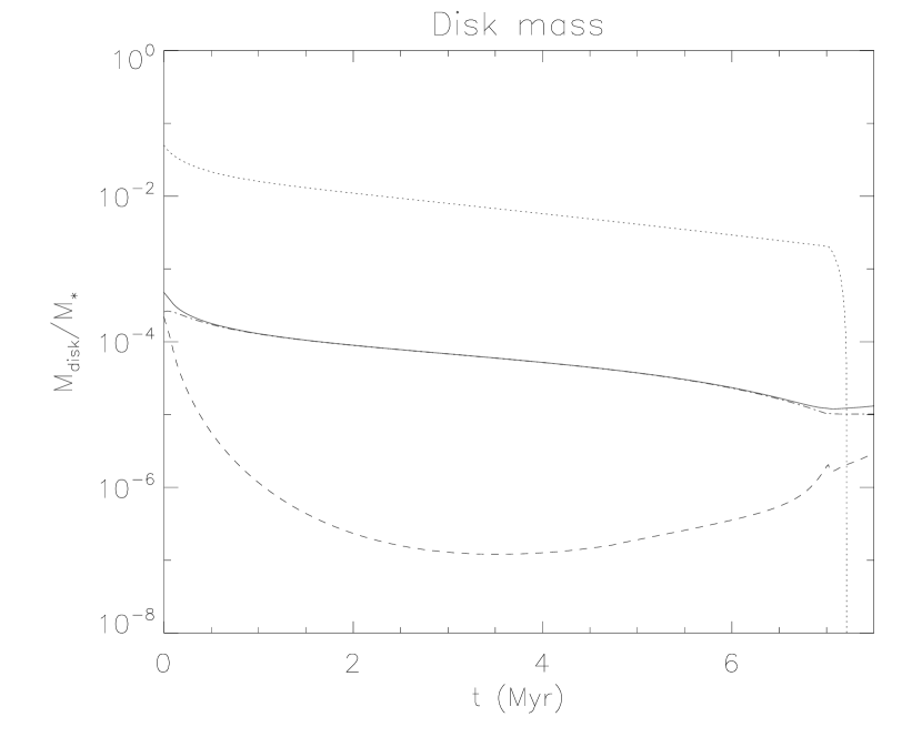
Figure 5: Total disk mass in the fiducial model. The dotted line shows the integrated gas mass and the solid line shows the integrated solid mass. To illustrate the rapid loss of solids in the inner disk, the total disk mass contained in $r<20$AU is shown in the dashed line, while the rest is shown in the dot-dash line.

4.1 Evolution of the gas surface density

The characteristic evolution of $\Sigma(r,t)$ under this particular photo-ionizing wind model has been extensively studied by Alexander, Clarke, & Pringle, (2006a and 2006b) (see also Clarke, Gendrin & Sotomayor, 2001). It can be seen in Figure 3 as a dotted line, and in more detail in Figure 6. While the mass flux from photo-evaporation is negligible compared with the mass flux from viscous accretion/spreading, the disk undergoes a long period of near self-similar evolution. When both fluxes become comparable a depression appears in $\Sigma(r,t)$ and a gap eventually forms, here at radius $r_{\rm gap}=0.9$ AU, at $t=7$Myr. Within a few thousand years, most of the gas in the inner disk has been accreted onto the central star, while the radius of the hole begins to expand as a result of direct photo-evaporation. At $t=7.12$Myr, the hole radius has retreated to 200AU, and finally beyond 500 AU after $t=7.19$Myr.

While the evolution of the gas is (in this model) independent of the evolution of solids, particle growth and particle migration are nonlinearly strongly coupled.

4.2 Particle growth

The evolution of the maximum particle size $s_{\rm max}(r,t)$ is shown in Figure 4a both for very early times and at later times. Grain growth is extremely rapid in the inner disk regions in the early stages of disk evolution, in particular near sublimation lines. Within just 100,000 yr, a characteristic shape to the curve $s_{\rm max}(r,t)$ appears, which contains three different regions: (I) in the innermost disk region ($r$ smaller than a fraction of 1 AU), a slightly tilted plateau corresponding to the particles having reached isolation mass; (II) a power-law region (from a fraction of 1 AU to about 100AU); (III) a region where grains have undergone negligible growth. Superimposed on this characteristic shape are a set of peaks corresponding to the successive sublimation lines. The transition between region I and region II is easily identified as the transition between the gravitational regime and the turbulent regime; its steepness confirms that as soon as gravitational focusing becomes effective, the collision rate increases and particles rapidly reach isolation mass. The transition between region II and region III can also be easily identified as the region where the growth timescale of particles of size $s_{\rm max0}$ becomes comparable with the age of the disk.

Once established (after the first Myr), the global shape of the curve $s_{\rm max}(r,t)$ varies little with time (see solid lines), although particles within the sublimation region continue growing, and the three regions slowly expand outward.

4.3 Solid density and chemical composition

The evolution of the solid density is shown in Figure 3. Small particles well-coupled with the gas ($St_{\rm max}\ll 1$) closely follow its inward or outward motion depending on the radial position considered. As a result, during the initial viscous spreading of the disk (within the first Myr) a significant proportion of the mass in solids is transported outward with the gas creating a large reservoir of small dust grains at large radii ($r>100$AU). Meanwhile, particles in the inner regions of the disk ($r<10$ AU) rapidly grow and begin to drift towards the central star differentially from the gas, which results in local changes in the metallicity $\Sigma_{\rm p}/\Sigma$. Figure 4b shows the evolution of metallicity in more detail, and reveals that the inner and intermediate disk go through an initial phase of strong depletion in heavy elements. Later, the global evolution of the surface density of particles is controlled by the mass flux incoming from large radii. The observed increase in the metallicity is essentially related to the decrease in $\Sigma$ through photo-evaporation.

In addition to this global trend strong surface density peaks can be observed near the successive sublimation lines. These are presumably caused by the differential drift of the solid and vapor form of each chemical species (Stepinski & Valageas 1997, Ciesla & Cuzzi, 2006). The peaks consistently stand roughly one to two orders of magnitude above the smoother “background” surface density profile, but do not appear to grow independently of it beyond the first 100,000 yrs. As the gas density decreases, the local metallicity near the sublimation lines steadily grows. By 4Myr, the sublimation line for refractory materials has equal content in gas and solids, suggesting the possibility of local onset of gravitational instability of solids (which is not modeled here). After 6Myr, the two remaining sublimation lines (for the volatile and iron-rich material) also pass the same threshold. Interestingly, Figure 3 reveals that the very rapid growth of material near each sublimation line traps a variety of grain species into the growing bodies, so that the strong enhancement in the surface density of icy bodies near the volatile sublimation line is accompanied by an enhancement in the surface density of refractory materials and iron-rich materials. The same phenomenon is observed near the sublimation line for refractory materials.

4.4 Disk masses

The evolution of the total mass in gas and solids in the disk is shown in Figure 5 as dotted and solid lines respectively. Also shown are the total amount of solids found within 20 AU and outside of 20AU. At $t=0$, the solid mass is equally distributed between the inner ($<20$ AU) and the outer disk ($>20$AU); Within a short time (of the order of 100,000yr), most of the mass in the inner disk accretes onto the central star, while the mass contained in the outer disk remains at a constant fraction of the disk mass in gas. Beyond this point, the mass in the inner disk is controlled by the flux of material drifting in from the outer disk.

When the gap opens (at 7Myr), the total mass of gas drops precipitously (within about 200,000 yr) while the total mass of solids remains constant. The total content of solids left in the disk after complete photo-evaporation of the gas is about 1.3 $\times 10^{-5}M_{\odot}$, or in other words about 4 Earth masses. Only 20% of this amount is located within the inner 20AU of the disk, while the remaining 80% are swept out to the outer disk.

5 Mathematical interpretation of the results

In order to gain more insight into the numerical results for the fiducial model, it is useful to characterize and when possible quantify some of the generic behaviors observed in the solutions.

In this section I present both existing and new analytical results on the evolution of gas and solids in viscously evolving disks. While the complexity of the system clearly precludes the existence of a closed-form fully analytical solution, there are certain limits where analytical efforts pay off. By comparing the analytical estimates derived with the exact outcomes of the numerical algorithm, I am able to test the numerical results on a systematic basis, and at the same time obtain strict constraints on the regimes of validity of the analytical solutions.

Given that the evolution of the gas is more-or-less independent of the evolution of solids, much progress has already been done in describing it analytically. These are presented in §5.1. New results on the evolution of solids are presented in §5.2 and §5.3.

5.1 Evolution of the gas

The evolution of the gas density is shown in more detail in Figure 6. Lynden-Bell & Pringle (1974) (see also Hartmann et al. 1998) showed that provided (i) the mass accretion rate due to viscous transport is much larger than the wind photo-evaporation rate and (ii) the disk is allowed to spread to infinity, then there exist a simple self-similar solution for $\Sigma(r,t)$:

$$\Sigma(r,t) = \frac{M_{0}}{2\pi rR_{0}}T^{-3/2}\exp\left(-\frac{r}{R_{0}T}\right)\mbox{ with }$$

$$T = \frac{t}{\tau_{\rm v}}+1\mbox{ , }$$ (55)

where the viscous spreading time of the disk is $\tau_{\rm v}=R_{0}^{2}/3\nu_{\rm t}(R_{0})$. In this solution, the gas velocity is equal to

$$u=-3\nu_{\rm t}(r)\left(\frac{1}{2r}-\frac{1}{R_{0}T}\right)$$ (56)

showing that $u<0$ for $r<r_{\rm v}(t)$ (viscous accretion) and $u>0$ for $r>r_{\rm v}(t)$ (viscous spreading), the critical radius being $r_{\rm v}(t)=R_{0}T/2$.

Figure 6: Gas surface density in the fiducial model (from the top to the bottom curve) at $t$ = 0, 1, 2, 3, 4, 5, 6 and 7 Myr. The solid lines show the exact numerical solution, while the dotted lines show the analytical estimate provided by the self-similar solution (55) at the same times.

Figure 6 compares the self-similar solution compares with the true numerical solution, and reveals excellent agreement at early times, gradually deteriorating in the inner disk as time evolves and photo-evaporation begins to dominate the gas dynamics. In the outer disk the agreement remains globally much better (since the photo-evaporation rate is very low at large radii) and deteriorates only slightly (by a factor of no more than a few) as expected when the critical radius reaches the outer boundary. Note that a much better approximation to $\Sigma(r,t)$ including the effects of photo-evaporation has been obtained by Ruden (2004).

In the early self-similar phase, and within $r_{\rm v}$, the mass accretion rate $\dot{M}(r,t)=2\pi ru\Sigma$ is roughly constant with radius. The total gas disk mass decays as $M(t)=M_{0}T^{-1/2}$ (neglecting the effects of the outer boundary condition), so that the gas accretion timescale increases linearly with the reduced time: $M/|\dot{M}|\simeq 2T\tau_{\rm v}$.

When the photo-evaporation rate becomes comparable with the accretion rate, a gap opens in the disk. Hollenbach et al. (1994) argued that the gap opening radius $r_{\rm gap}$ is located close to the gravitational radius $r_{\rm g}=GM_{\star}/c_{i}$, while Liffman (2003) and Font et al. (2004) revised this estimate to be a fraction of $r_{\rm g}$. Since $r_{\rm g}$ scales linearly with stellar mass so does $r_{\rm gap}$; in what follows, I adopt

$$r_{\rm gap}=1\left(\frac{M_{\star}}{M_{\odot}}\right){\rm AU}\mbox{ . }$$ (57)

The time at which the gap opens can be estimated by equating the wind mass loss rate $\dot{M}_{\rm w}$ to the viscous accretion rate in the self-similar solution (Clarke, Gendrin & Sotomayor, 2001); this yields (provided $\tau_{\rm gap}\gg\tau_{\rm v}$)

$$\tau_{\rm gap}=\tau_{\rm v}\left(\frac{M_{0}}{2\tau_{\rm v}\dot{M}_{\rm w}}\right)^{2/3}\mbox{ . }$$ (58)

The wind mass loss-rate prior to gap opening for the fiducial model was calculated by AA07 to be

$$\dot{M}_{\rm w}\simeq 4\times 10^{-10}M_{\odot}\mbox{/yr}\mbox{ . }$$ (59)

Table 3 compares the estimate from equation (58) with the outcome of numerical simulations with varying $R_{0}$ and $M_{0}$, showing that it is indeed a very good estimate for the gap formation timescale except for the fiducial model. This is because the actual viscous mass accretion rate in the numerical solution of the fiducial model deviates from the simple estimate of $M_{0}T^{-3/2}/2\tau_{\rm v}$ at large times, when the disk spreads all the way out to the outer edge of the numerical mesh.

Table 3: Gap opening time, actual and predicted

$R_{0}$ (AU) $M_{0}/M_{\odot}$ $\tau^{\rm num}_{\rm gap}$ (Myr) $\tau^{\rm pred}_{\rm gap}$ (Myr) 30 0.05 7.01 7.79 10 0.05 5.35 5.40 5 0.05 4.36 4.29 10 0.01 1.96 1.84


After the gap formation, supply of material from the outer disk is shut off and the inner disk rapidly clears of all gas. The gas clearing time can be estimated from the viscous timescale at the gap formation radius:

$$\tau_{\rm clear}=\tau_{\rm v}\left(\frac{r_{\rm gap}}{R_{0}}\right)\mbox{ . }$$ (60)

In the fiducial model, the gas clearing time is of the order of 4,000 yr only, and can be considered to be near-instantaneous. This is indeed seen in the simulations (see Figure 3).

Direct photo-ionization of the gas at the hole edge results in a sharp change in the gas mass loss rate (see Appendix A). The evolution of the size of the hole can be derived from the work of Alexander, Clarke & Pringle (2006b) to be

$$r_{\rm hole}(t)=r_{\rm gap}\left(\frac{t-\tau_{\rm gap}}{2\tau_{\rm clear}}+1\right)^{2}\mbox{ , }$$ (61)

which is again a good estimate of the hole radius derived from the numerical solution (see §4.1) for $t>\tau_{\rm gap}$.

5.2 Grain growth

For simplicity, in this section I focus on deriving analytical estimates for grain growth in disks where sublimation and condensation are neglected. For ease of comparison with the numerical model, an additional run was performed using the fiducial model but with no sublimation or condensation of material, yielding the solution shown on Figure 7. After the initial rapid growth period (for t ¿ $10^{4}$ yrs), one can note very clearly the three regions of interest described earlier: region III where $s_{\rm max}(r,t)\simeq s_{\rm max0}$; region II where $s_{\rm max}(r,t)$ appears to follow roughly a power law in $r$, and region I where the particles have reached isolation mass and stopped growing. In this figure the peaks associated with sublimation lines are naturally absent.

Figure 7: Maximum grain size $s_{\rm max}(r,t)$ at $t=0$, 1, 10, 100, 1000, $10^{4}$, $10^{5}$ and finally $10^{6}$ yrs (solid lines, from bottom to top) obtained from the numerical simulation of the fiducial model with no sublimation/condensation. The dotted lines show the analytical estimates of equation (65) at the same times. The dashed line marks the transition between the turbulent and gravitational regime at $t=1$Myr.

Despite the apparently simple behavior of the numerical solutions, modeling this evolution is a complex problem: the particle growth rate depends on $\Sigma_{\rm p}(r,t)$, which is regulated by the drift velocity of the particles, which depends on the particle size $s_{\rm max}(r,t)$. The implied nonlinearities preclude the existence of analytical solutions in most cases.

However, there exist a limit in which insight can be gained from simple models: when the particle drift time is much longer than the particle growth time, one can expect the metallicity to remain close to its initial value, namely $\Sigma_{\rm p}/\Sigma=Z_{0}$. This happens in the very early stages of disk evolution (the limit of small $t$), as well as in the outer regions of the disk (region III) at all times.

5.2.1 Growth timescales

To interpret the numerical solutions I consider the growth regime dominated by turbulent encounters, where particles of size $s_{\rm max}$ follow the growth law given by equation (36). The growth timescale of the particles is given by

$$\tau_{\rm g}=\left(\frac{1}{s_{\rm max}}\frac{{\rm d}s_{\rm max}}{{\rm d}t}\right)^{-1}\mbox{ . }$$ (62)

In the limit where $St_{\rm max}\ll 1$, the growth timescale is equal to

$$\tau_{\rm g}=\frac{\Sigma}{\Sigma_{\rm p}}\sqrt{\frac{St_{\rm max}}{\alpha_{\rm t}}}\frac{\tau_{\rm d}}{\epsilon}\mbox{ , }$$ (63)

while in the limit where $St_{\rm max}\gg 1$

$$\tau_{\rm g}=2\sqrt{3}\gamma^{1/4}\frac{\Sigma}{\Sigma_{\rm p}}St_{\rm max}^{3/4}\frac{\tau_{\rm d}}{\epsilon}\mbox{ . }$$ (64)

Note that the second expression is independent of $\alpha_{\rm t}$. This is related to the fact that for larger particles, coupling with the turbulent eddies is weakened, which reduces their relative velocities but also increases particle concentration through sedimentation.

Figure 8: Growth timescale for particles of size $s$ for the initial conditions of the fiducial disk described in §3.2 with no sublimation/condensation; the curves show the growth timescale at $r$ = 0.1AU (solid line), $r=$ 1AU (dotted line), $r=$ 10AU (dashed line) and finally $r=$ 100AU (dot-dash line). The symbols show the true $s_{\rm max}(r,t)$ at the same radii (0.1 AU: diamonds; 1 AU: stars; 10 AU: triangles; 100 AU: squares).

Figure 8 shows (as lines) the exact analytical expression for the growth timescale obtained by combining equation (62) with equation (36), and considering $\Sigma_{\rm p}/\Sigma$ fixed and equal to the initial metallicity $Z_{0}=0.01$. Growth timescales of particles at radii 0.1, 1, 10 and 100 AU are shown. The power laws seen in either limits are well-approximated by equations (64) and (63), and the flattening of the four curves corresponds to the transition $St_{\rm max}\ll 1$ to $St_{\rm max}\gg 1$. This figure is particularly useful for reading directly the maximum size of particles achievable at a given age in the disk should the surface densities of dust and gas indeed remain constant over that period. For example by looking at the intersection of a horizontal line at $10^{4}$yr with each curve, one deduces that in a $10^{4}$yr-old disk there will be no significant growth beyond 20 AU, 10-20$\mu$m-size particles at 10AU, m-size objects at 1 AU and finally, gravitationally dominated growth (towards isolation mass) below 0.1AU. Since $\tau_{\rm g}\propto 1/Z_{0}\epsilon$, the growth timescale and maximum particle sizes for disks with other values of the metallicity $Z_{0}$ or sticking efficiency $\epsilon$ can be read by translating the curves up or down accordingly.

In reality, the metallicity $Z=\Sigma_{\rm p}/\Sigma$ is of course not constant. Figure 8 also shows (as symbols) the actual particle size achieved in the fiducial disk with no sublimation/condensation at the same selected radii. The lines and the symbols follow each other reasonably well in the expected limits (large radii or short times) up to the point where $St_{\rm max}\simeq 1$ at which point the simple analytical estimate systematically breaks down.

5.2.2 Particle size

Given the good fit found for particles with $St_{\rm max}\ll 1$, I now approximate $s_{\rm max}(r,t)$ by the value of the grain size for which the growth timescale equals the age of the disk: setting $\tau_{\rm g}=t$ in equation yields (63)

$$s_{\rm max}(r,t)=\frac{\sqrt{2\pi\gamma}}{\rho_{\rm s}}\left(\frac{t}{{\rm 1year}}\right)^{2}\left(\frac{\Sigma_{\rm p}}{\Sigma}\right)^{2}\epsilon^{2}\alpha_{t}\Sigma(r,t)r_{\rm AU}^{-3}\left(\frac{M_{\star}}{M_{\odot}}\right)\mbox{ . }$$ (65)

If one assumes as before that $\Sigma_{\rm p}/\Sigma\simeq Z_{0}$ then one can get a rough estimate of $s_{\rm max}(r,t)$ by combining equations (65) and (55), and shown in Figure 7 as dotted lines.

As expected, the estimate for $s_{\rm max}(r,t)$ is in fairly good a agreement with the numerical results for small times; it correctly predicts the power law structure of the whole intermediate region (for $s<1$km, roughly) at early times (t ¡ $10^{4}$yr), but not so at later times (where the analytically predicted power law is too steep compared with the numerical results). This is again related to the fact that the surface density of particles becomes significantly depleted at later times.

The estimate for $s_{\rm max}(r,t)$ also correctly predicts the transition between regions II and III of the disk. Since particle growth is fundamental to our understanding of disk SEDs, I now give an analytical estimate for this transition radius: for early times (for $t<\tau_{\rm v}$), $r^{II}_{III}(t)$ is given by

$$r^{\rm II}_{\rm III}(t)=\left[\frac{Z_{0}^{2}\epsilon^{2}\alpha_{\rm t}}{St_{\rm max0}}\frac{R_{0}}{1{\rm AU}}\right]^{1/4}\left(\frac{t}{1{\rm year}}\right)^{1/2}\left(\frac{M_{\star}}{M_{\odot}}\right)^{1/4}{\rm AU}\mbox{ , }$$ (66)

where

$$St_{\rm max0}=\frac{2\pi R_{0}^{2}s_{\rm max0}\rho_{\rm s}}{\sqrt{2\pi\gamma}M_{0}}$$ (67)

is the Stokes number at $t=0$ and $r=R_{0}$ of particles of size $s_{\rm max0}$. For later times ($t>\tau_{\rm v}$)

$$r^{\rm II}_{\rm III}(t)=\left[\frac{Z_{0}^{2}\epsilon^{2}\alpha_{\rm t}}{St_{\rm max0}}\frac{R_{0}}{1{\rm AU}}\right]^{1/4}\left(\frac{\tau_{\rm v}}{1{\rm year}}\right)^{3/8}\left(\frac{t}{1{\rm year}}\right)^{1/8}\left(\frac{M_{\star}}{M_{\odot}}\right)^{1/4}{\rm AU}\mbox{ . }$$ (68)

5.2.3 Gravitational regime

The transition from the turbulent regime to the gravitational regime (region II to region I) is easily understood by considering equation (45). The transition size $\tilde{s}_{\rm max}$ is given by

$$\tilde{s}_{\rm smax}(r,t)=7.1\left(\frac{M_{\star}}{M_{\sun}}\right)^{10/51}\left(\frac{h}{r}\right)^{8/17}\left(\frac{\Sigma(r,t)}{1000{\rm g/cm}^{2}}\right)^{7/17}{\rm km.}$$ (69)

The curve for $\tilde{s}_{\rm smax}(r,t)$ at $t=$1Myr is shown on Figure 7, and correctly marks the transition between the turbulent and gravitational regime at the time considered. As time progresses and $\Sigma(r,t)$ decreases so does the transition size.

5.3 Evolution of the solid mass fraction prior to gap opening

The evolution of the solid mass fraction is governed by particle diffusion and drift. The analytical prescription used to describe the particle size distribution function is particularly useful since it can easily be integrated to yield the bulk motion properties, as seen in equations (20) and (50). Given the asymptotic behavior of the functions $I(x)$ and $J(x)$, $u_{\rm p}$ is roughly equal to

$$u_{\rm p} = u-2\eta v_{\rm K}\frac{2\pi St_{\rm max}}{3}\mbox{ for }St_{\rm max}\ll 1\mbox{ , }$$

$$u_{\rm p} = (u-2\eta v_{\rm K})\frac{\sqrt{\pi}}{4\sqrt{St_{\rm max}}}\mbox{ for }St_{\rm max}\gg 1\mbox{ , }$$ (70)

so that, as expected, the bulk radial velocity of the particles is close to that of the gas for small particles, and tends to $0$ when $s_{\rm max}$ grows. Note that $u_{p}\propto 1/\sqrt{St_{\rm max}}$ instead of $1/St(s)$, which accounts for the fact that even though particles of size $s_{\rm max}$ may be largely decoupled from the gas, a non-negligible mass fraction is contained in rapidly drifting intermediate-size particles. This is the main difference between this model and a single-size particle model; it accounts for the fact that even when $St_{\rm max}\gg 1$, a significant fraction of the collisional encounters are destructive and result in the erosion of the larger bodies into smaller rapidly drifting particles with $St(s)\simeq 1$.

5.3.1 Reservoir of small grains at large radii

The sign of $u_{\rm p}$ determines whether grains are transported inward or outward. As expected from equation (56) the gas velocity changes sign at $r_{\rm v}(t)$. This critical radius grows linearly with $T$ (defined in equation (55)), and therefore sweeps outward roughly on the viscous timescale $\tau_{\rm v}$. As a result for $r<r_{\rm v}$ the particle velocity is necessarily negative, while for $r>r_{\rm v}$ particles can be entrained outward provided they are strongly coupled with the gas. Since $r_{\rm v}$ is typically much larger that $r^{\rm II}_{\rm III}$, all the particles outward of $r_{\rm v}$ are particles of size $s_{\rm max0}$. Combining these facts implies that there exists a reservoir of small particles at large radii, slowly eroded by the outward motion of $r_{\rm v}(t)$. In addition, as the gas density drops, the small particles gradually decouple from the gas implying that the reservoir begins to “leak”. Eventually, even the smallest particles decouple from the gas, and all the solids come rushing inward. The evolution of the particle velocity can be seen in Figure 9. Note the existence of the reservoir (a region of significant radial extent with $u_{\rm p}>0$) for all particle sizes at early time. As time progresses, the reservoir begins to “leak” as the particles gradually decouple from the gas, until a a critical point where $u_{\rm p}$ becomes negative for all radii. The phenomenon depends strongly on the initial size of the particles $s_{\rm max0}$: three simulations are shown in which the maximum particle size is respectively $1\mu$m, $3\mu$m and $10\mu$m. The timescale $t_{\rm p}$ for the release of the particle reservoir is clearly much shorter for the larger particles (0.84Myr for 10$\mu$m-size particles instead of 2.33Myr for $\mu$m-size particles).

Figure 9: Radial velocity $u$ of the gas (solid line) and mass-weighted average radial velocity $u_{\rm p}$ of particles of maximum size $s_{\rm max0}=1\mu$m (dotted line), $3\mu$m (dot-dashed line) and $10\mu$m (dashed line). Note how the slow erosion and eventual release of the reservoir (i.e. of the spatial region with $u_{\rm p}>0$) depends on $s_{\rm max0}$.

In fact, this timescale can easily be estimated by solving simultaneously the equations $u_{\rm p}=0$ and $\partial u_{\rm p}/\partial r=0$. Assuming that $\Sigma(r,t)$ is equal to the self-similar solution, and that the particles in that regime satisfy $St_{\rm max}\ll 1$ (which was checked numerically), $u_{p}\simeq u-4\pi\eta St_{\rm max}/3$. It follows that

$$\frac{t_{\rm p}}{\tau_{\rm v}}+1=T_{\rm p}=\left[\frac{3}{16e\pi^{2}\eta(R_{0})}\frac{\tau_{\rm d}(R_{0})}{\tau_{\rm v}}\frac{1}{St_{\rm max0}}\right]^{2/5}\mbox{ , }$$ (71)

where $\tau_{\rm d}(R_{0})$ is the dynamical time at $R_{0}$, $\eta(R_{0})$ is obtained by applying equation (48) at $r=R_{0}$, $St_{\rm max0}$ is the Stokes number of particles of size $s_{\rm max0}$ at $R_{0}$ (see equation (67)). Note that in order to derive this expression, I have also made explicit use of the fact that $q=-1/2$. The quality of this estimate is found to be excellent given the approximations made (see Figure 10), and small discrepancies are attributed to the fact that $\Sigma(r,t)$ is not exactly equal to the self-similar solution, and that $u_{\rm p}$ has been approximated by its Taylor expansion for small $St_{\rm max}$. In the same analytical calculation, the radius of the reservoir at release is found to be $r_{p}=R_{0}T_{p}$; checking this solution against the numerical runs also reveals excellent agreement.

Figure 10: Non-dimensional timescale $T_{p}$ for the release of the particle reservoir as a function of initial particle size $s_{\rm max0}$. The analytical estimate (solid line) is compared with hand-checked values of $T_{\rm p}$ for three numerical simulations of the fiducial model with different initial particle sizes (stars). On the same plot is shown the numerically determined radius of the reservoir at release $r_{p}$ in AU (diamonds) as well as the corresponding analytical estimate $R_{0}T_{p}$ (dashed line).

5.3.2 Evolution of the total mass of the particle disk

Since particles in the inner disk can achieve significant sizes, the drift timescale of grains within $r_{\rm v}(t)$ is usually much smaller than the viscous accretion timescale and/or the age of the disk. This can be readily seen in Figure 9.

This very simple fact has important consequences: it implies that the distribution of solids in the inner disk is uniquely controlled by the mass flux leaking from the reservoir. One way to see this is to look at the particle disk evolution timescale $M_{\rm p}/|\dot{M}_{\rm p}|$ obtained by numerical integration of the fiducial model. Figure 11 shows results for the three different initial particle sizes considered in the previous section (as solid lines). The linear increase for early times ($T\ll T_{\rm p}$) mirrors the gas evolution timescale, as expected from the tight coupling between the reservoir particles and gas:

$$\dot{M}_{\rm p}(t)=Z_{0}\dot{M}(t)=-\frac{Z_{0}M_{0}}{2\tau_{\rm v}}T^{-3/2}\mbox{ , }$$ (72)

so that $M_{\rm p}/|\dot{M}_{\rm p}|\simeq M/\dot{M}=2\tau_{\rm v}T$. As $T$ exceeds $T_{\rm p}$, the linear increase saturates then rapidly turns over, as expected from the release of the reservoir particles.

Constructing an exact analytical model governing the evolution of the particle disk after $T_{\rm p}$ from first principles turned out to be rather difficult. However, it is possible to gain insight into the problem by inspecting the results of the numerical simulations first. At later time, one can expect the dynamics of the particle disk to depend on the reservoir release timescale $T_{\rm p}$. I seek a functional form of the kind

$$\frac{M_{\rm p}}{\dot{M}_{\rm p}}\simeq 2\tau_{\rm v}Tf\left(\frac{T}{T_{\rm p}}\right)\mbox{ , }$$ (73)

with

$$f(x)=\frac{e^{-a_{1}x}}{1+a_{2}x^{a_{3}}}\mbox{ , }$$ (74)

(with $a_{1}$, $a_{2}$, $a_{3}>0$) which satisfies the requirement that $f(x)\rightarrow 1$ as $x\rightarrow 0$, and $f(x)\rightarrow 0$ nearly exponentially as $x\rightarrow\infty$). A fairly good (but clearly not perfect) fit for all three curves is empirically found to have $a_{1}=0.2$, $a_{2}=0.25$ and $a_{3}=3.3$, implying

$$\frac{{\rm d}{M}_{\rm p}}{{\rm d}t}\simeq-\frac{M_{\rm p}}{2T}\exp\left(0.2\frac{T}{T_{\rm P}}\right)\left(1+0.25\left(\frac{T}{T_{\rm P}}\right)^{3.3}\right)\mbox{ . }$$ (75)

The fitting curves, for each of the three initial particle sizes chosen, are also shown in Figure 11a. The initial linear rise as well as the maximum are very well represented, while the fit at later times (for $T>T_{\rm p}$), in particular for the smaller particle sizes, is slightly poorer. Integrating equation (75) yields an estimate for the total particle disk mass as a function of time, which is compared with the results of the numerical simulations in Figure 11b. The approximate solutions follow the trend of the exact solutions well, with some small acceptable systematic deviations at early times (see below). In particular, it reproduces well the very rapid decrease in the particle disk mass as the reservoir is finally released ($T>T_{\rm p}$).

Figure 11: Left figure: Particle disk evolution timescale $M_{\rm p}/|\dot{M}_{\rm p}|$. The solid lines are the outcomes of the numerical simulations for the fiducial model with initial particle sizes (from top to bottom) 1$\mu$m, 3$\mu$m and $10\mu$m respectively. The empirical analytical fits to these formula are also shown, with the dotted line for the 1$\mu$m case, the dot-dash line for the 3$\mu$m case and the dashed line for the 10$\mu$m case. Right Figure: Total mass in solids in the disk as a function of the nondimensional time $T$. The three solid lines are the outcomes of the numerical simulations for the fiducial disk model with initial particle sizes (from right to left) 1$\mu$m, 3$\mu$m and $10\mu$m respectively. Approximates to these numerical results are obtained by seeking the solution to equation (75), and also shown here (linestyles are the same as in the left-side figure).

A very important consequence of the “leaky reservoir” model is that the total disk mass is reasonably independent of the physical phenomena taking place in the inner disk (provided the bulk drift timescale of the particles is smaller than the viscous accretion timescale). This implies that the evolution of the total disk mass depends very weakly on the particle growth rate (and in particular of the sticking efficiency $\epsilon$), and of sublimation or condensation fronts. This can actually be seen in Figure 11, which shows the numerical solution for the fiducial model with sublimation/condensation in addition to the three curves discussed earlier. The disk mass in the fiducial model is practically indistinguishable from that of the disk without sublimation/condensation (for the micron-size particles).

Finally, note that the proposed evolution equation for $M_{\rm p}$ breaks down if the bulk drift timescale of the particles is comparable to or larger than the viscous accretion timescale or the age of the disk (whichever is smaller). For instance, if the particles remain small at all times, then they naturally follow the evolution of the gas at all times (which explains the results of AA07). As an other example, one can see in Figure 11 when $T\rightarrow 1$ that there is a very small difference between the fiducial model with sublimation/condensation lines and the model without. This arises because at early times, the drift timescale of the particles is much smaller than the age of the disk and the solid mass content has not yet had time to equilibrate. As a result, most of the solid mass in the inner disk rapidly drifts toward the central star. In the absence of sublimation lines all of this mass is lost, whereas a significant fraction of it can get trapped by the sublimation lines if sublimation/condensation is taken into account (see §5.5).

5.3.3 Evolution of the particle surface density

Having characterized the global evolution of the total disk mass in solids (which was shown to depend only on the initial grain size $s_{\rm max0}$ and on the viscous diffusion time $\tau_{\rm v}$), one could hope to describe the evolution of the surface density of grains as well. As mentioned earlier, when the surface density of grains within the disk is controlled by the mass flux coming from the reservoir one can expect that

$$2\pi ru_{\rm p}(r,t)\Sigma_{\rm p}(r,t)\simeq\dot{M}_{\rm p}(t)\mbox{ , }$$ (76)

where $\dot{M}_{\rm p}(t)$ is given by equation (75). This approximation turns out to be quite good (except outside of $r_{\rm v}(t)$ of course). Unfortunately, the problem lies elsewhere: even though $\dot{M}_{\rm p}(t)$ is known, it is particularly difficult to estimate $u_{\rm p}(r,t)$ since it depends on $s_{\rm max}(r,t)$ and $\Sigma(r,t)$: the analytical estimate of $s_{\rm max}(r,t)$ given in equation (65) is unfortunately not valid in regions I and most of region II beyond a few times $10^{4}$ yr and the self-similar solution for $\Sigma(r,t)$ is also invalid for $t>\tau_{\rm v}$ in the same regions. Using these estimates despite their poor quality yield predictions that are off by up to an order of magnitude (see Appendix C). Note that if all that is needed is a “quick and dirty” order of magnitude estimate then the procedure described in the Appendix could be considered satisfactory. In particular, it does reproduce well the particle surface density dip observed in the intermediate disk regions, a feature which could be used together with spatially resolved disk observations to constrain the value of the sticking efficiency $\epsilon$.

5.4 Evolution of the solids posterior to gap opening

The study of the evolution of solids after the gap opening phase was the main purpose of the work of AA07. When growth is ignored, AA07 showed that the evolution of the surface density of solids follows that of the gas (for small particles).

After the formation of the gap, both gas and solids within quickly accrete into the central star on the clearing timescale, leaving a hole clear of both dust and gas. Near the edge of the hole thus formed, an inversion in radial pressure gradient causes the particles to drift outward instead of inward. As the hole grows all of the grains outside of $r_{\rm hole}(t)$ are slowly shepherded outward with it. As a result of these processes, most of the solid mass at the time of gap opening is retained in the disk but moved to larger and larger radii.

When grain growth is taken into account on the other hand, a different picture emerges. The particles within the initial gap radius have typically grown to embryo sizes, so that their Stokes number is well above unity by the time the gap opens. The reduction in the surface density of the gas does not affect their drift velocity much (which is exactly the opposite case to the AA07 model) and they stay in place while the gas within the gap accretes. The “hole” thus created still contains a significant amount of solid material.

As direct photo-evaporation takes over, the hole in the gas widens as expected but the corresponding reverse radial pressure gradient has very little effect on the large particles. As a result, one observes a significant amount of solid material remaining in the inner disk all the way out to about 10 AU (in the case of the fiducial model). Eventually, the edge of the hole retreats out to regions where the particle Stokes number is of order unity, at which point the clearing begins as in the AA07 model. As already suggested by AA07, all particles smaller than 1-10cm are entrained to large radii, while all particles larger than this particular size remain behind.

The prediction for the particle size given in equation (65) can be used to estimate the radius outside of which particles are entrained, by setting the age of the disk to be $t=\tau_{\rm gap}$: let $r_{\rm inner}$ the innermost extent of the cleared region, so that

$$r_{\rm inner}=\left[\left(\frac{\tau_{\rm gap}}{1{\rm yr}}\right)^{2}Z_{0}^{2}\epsilon^{2}\alpha_{\rm t}\left(\frac{M_{\star}}{M_{\odot}}\right)\right]^{1/3}{\rm AU}$$ (77)

which yields a prediction of $r_{\rm inner}=16$ AU for the fiducial model. This value is larger than that observed in Figure 3 by a factor of about $2\simeq 10^{1/3}$, which can be attributed to the fact that the estimated particle size at this point is a factor of 10 too large compared with the true numerical simulations (see Figure 4). However, the estimate in equation (77) can be thought of as a solid upper limit for the radial extent of the remaining solid material in the inner regions of the disk after the clearing of the gas.

Material outside of $r_{\rm inner}$ is shepherded outward with the retreating hole. As more and more material is swept and entrained outward, a strongly localized surface density peak appears, which eventually grows to be a large as the local surface density of the gas. When this happens, two situations could occur within similar outcomes: either gravitational instabilities set in, resulting in the in-situ formation of a planet, or the frictional drag between the particles and the gas begins to influence the evolution of the gas itself, and the particles stop moving outward (neither effects are included in the numerical model, and therefore cannot be seen in the simulations). This effect is difficult to quantify in the general case, since neither $\Sigma_{\rm p}$ nor $\Sigma$ are known analytically at this stage of the disk evolution. In the fiducial model show in Figure 3, this occurs at about 200AU. This process could lead to the systematic formation of localized debris rings reasonably far from the central star (from a few tens to a few hundreds of AU), without any need for prior planet formation or other clumping mechanism. Such debris rings are commonly observed, or inferred from the dust dustribution (see for instance Schneider et al. 2006 for direct detections, and Strubbe & Chiang 2006 for inference from spatial dust distribution).

As in the AA07 model, most of the solid content present in the disk at $t=\tau_{\rm gap}$ remains in the disk after complete clearing of the gas. The fraction of solid material moved to large radii depends on the details of the surface density distribution of particles at $\tau_{\rm gap}$ (which is not well-known a priori), but is typically of the order of 80%-90% of the total mass of solids; the remaining fraction can be found in the inner disk.

5.5 Effects of sublimation and condensation

The role of sublimation lines on the local accumulation and growth of particles has already been shown and discussed by others (Stepinski & Valageas, 1997; Ciesla & Cuzzi, 2006). Roughly speaking, the idea is that particles composed mainly of a given chemical species drift inward until they reach the sublimation line where they are transformed into vapor. The vapor diffuses inward much more slowly than the rate of migration of the incoming solids, leading to a large enhancement of the local metallicity. Through turbulent diffusion, a fraction of the vapor content actually finds it way back through the sublimation line and recondenses. The typical width of the region where this effect dominates can be evaluated from a local diffusive lengthscale, and naturally scales as $h(r)$. The exact amount of material accumulating in the region is more difficult to estimate a priori, since it depends on the difference between the solid mass flux into the sublimation line and the vapor mass flux out of the sublimation line. However, for most of the lifetime of the disk the flux of both solid and gaseous material is controlled by the reservoir at large radii so that the solid mass flux is equal to $Z_{0}\dot{M}$, which is also roughly equal to the mass flux of vapor out of the sublimation zone. This explains why the relative strength of the surface density peaks compared with the background curve fails to grow with time after the initial adjustment period, which would necessarily occur otherwise.

The conclusion is that any local surface density enhancement, and associated localized peak in the particle size is created very early in the lifetime of the disk (this is indeed seen in Figure 4b) – but it is only later, when the gas surface density decays and the metallicity increases, that gravitational instabilities in the particle layer could set in to trigger the planetary formation process. This picture, should it be correct, also implies that the relative heights of the peaks determines a strict sequence of “alarm clocks” on planetary formation timescales.

Note that only three species have been selected in the fiducial model. Clearly, there will be as many surface density and particle size peaks as the number of separate sublimation temperatures. Also, in this particular model the background temperature of the disk is fixed. In reality, the disk temperature cools significantly as $\dot{M}$ decreases, resulting in the inward migration of the various sublimation lines (see Garaud & Lin 2007, for instance). This will also affect the shape of the surface density profile in the inner disk; feedback between the disk temperature profile and the evolution of the surface density of grains will be the subject of future work.

6 Discussion

6.1 Discussion of the particle size distribution function.

The fundamental assumption underlying this work is that of the maintenance of a power-law particle size distribution function at all radii, throughout the disk lifetime. The assumption is justified exactly only if the collisional timescale (note: not the growth timescale, which is naturally a factor of $1/\epsilon$ larger) is shorter than the drift timescale for each size-bin. Whether this is in fact exactly true is certainly unlikely, but neither is it particularly relevant. The correct questions that should be asked are: (i) how far from equation (8) is the true size-distribution function in a disk, and (ii) how do deviations from (8) impact the conclusions from this paper?

Question (i) is a fundamental question, with implications reaching far beyond the scope of this paper. Attempts at answering it have come from various angles including both direct observations (in disks, but also in molecular clouds, in the ISM, as well as in our own solar system) and numerical experiments. As mentioned in §2.3, the observational evidence and theoretical motivation for a power-law size-distribution function is strong but limited to more-or-less spatially isotropic and homogeneous cases where there exist no systematic size-dependent drift or settling velocity which could act as a size-filter. Numerical simulations of the coagulation-shattering balance in similar conditions also unanimously agree on the power-law distribution, with indices varying slightly depending on the model assumptions but never straying too far from -3.5.

Unfortunately, there has only been one study (Suttner & Yorke 2001) that self-consistently includes a complete parameterization of the coagulation/shattering balance together with radial drift and vertical settling of the particles in an accretion disk. Suttner & Yorke (2001) studied the formation of a protostellar accretion disk through the collapse of a uniformly rotating molecular cloud core, and closely followed the evolution of the grain size distribution function at every spatial position throughout the collapse phase (first 10,000 years). They found that accretion shocks play an important role in limiting the growth of the grains; they also found, as expected, that the assumed sticking efficiency essentially governs the maximum grain size achievable. The dust size distribution functions computed vary strongly with height above the disk: they show clear evidence that larger grains tend to be found in the mid-plane, while regions high above the mid-plane remain close to the MRN-derived initial conditions. This can be attributed to a combination of settling of the larger grains as well as preferential in-situ growth. The mid-plane regions in their simulations appear to be largely depleted of small grains, which would be evidence for strong deviations from the power-law structure I assume. However, one may wonder whether this depletion is indeed true in a real disk, since Suttner & Yorke neglect diffusion of the smallest grains by the gas turbulence (which could easily bring small grains back towards the mid-plane from higher regions of the disk).

In conclusion, one should bear in mind that the assumption made in selecting a power-law size distribution function is probably not always strictly justified (in particular for larger particles). But given the enormous computational advantage of this approach, it should be thought of as an acceptable trade-off between models in which the full coagulation/shattering equation is solved, and models in which only one particle size (or a few particle sizes) are considered.

Question (ii) can easily be answered by identifying where in the proposed model the assumption of a power-law size-distribution function is used.

As mentioned in §2.5, the minimum particle size $s_{\rm min}$ plays no role in the dynamical evolution of the solids in the disks, as long as $s_{\rm min}\ll s_{\rm max}$, which is the case for the MRN size-distribution function, and therefore likely to continue being the case throughout the disk evolution. Thus whether the smallest grains are slightly depleted or not compared with the proposed power-law distribution function really does not matter.

Collisional growth is essentially dominated by encounters between particles of similar sizes: even if collisions with smaller particles are more frequent, the mass gained is much smaller. This is easily seen mathematically in the derivation of the growth rates ${\rm d}s_{\rm max}/{\rm d}t$ in §2.5, where the integral over all possible impactor sizes is always dominated by the largest particles, except possibly when $St_{\rm max}\gg 1$, in which case the integral is dominated by particles of intermediate size. Another way of seeing this is that while the assumptions concerning the grain size distribution function used to derive equation 36 are very different from those of Stepinski & Valageas (1997) who assume that the distribution function is strongly peaked around a single-size, the outcome is the same whithin some factors of order unity.

The systematic radial motion of decoupled particles ($St_{\rm max}\gg 1$) is the only place where the assumption made has a significant effect on the model results. If one assumes that all particles have a single size $s_{\rm max}$, then $u_{\rm p}(s_{\rm max})\propto 1/St_{\rm max}$ while if one considers the mass-weighted average motion of all particles following the proposed size-distribution function (8) then $u_{\rm p}\propto 1/\sqrt{St_{\rm max}}$ which can be significantly larger. As mentioned earlier, this accounts for the fact that when a continuum of particle sizes is taken into account, intermediate-size grains (with $St(s)\simeq 1)$) do rapidly drift leading to a non-neligible mass flux, even if the largest ones are fully decoupled,

The scaling $u_{\rm p}\propto 1/\sqrt{St_{\rm max}}$ clearly depends on ${\rm d}n/{\rm d}s\propto s^{-3.5}$; whether this exact scaling really applies to disks certainly is debatable, but I would argue that the general picture of large bodies being eroded by collisions and leading to a non-negligible mass-flux even when the larger bodies themselves do not drift has to hold. The only caveat is that the collision rate becomes null when the bodies reached isolation mass; thus one should, for self-consistency, set $u_{\rm p}\rightarrow 0$ in this limit, which was not done here (otherwise, smaller particles coming from larger radii artificially accumulate in the inner regions). A way forward would be to combine the model proposed here with an N-body code, in which particles are treated using a size-distribution until they reach embryo size, then taken out of the distribution and individually followed using N-body simulations. This could be the subject of future work.

6.2 Heavy element retention efficiency in the UV-switch model

The simple equation for the evolution of the total mass of solids (75) can be used to derive the final contents of the disk after complete gas dispersal when caused by photo-evaporation from the central star.

If grains in the outer disk remain fully coupled to the gas throughout the lifetime of the disk (i.e. if $t_{p}\gg\tau_{\rm gap}$, or equivalently, $s_{\rm max0}\ll 1\mu$m) then the amount of material left after complete dispersal of the gas can easily be estimated by the amount of solids left at $t=\tau_{\rm gap}$ (see AA07). Therefore an order of magnitude estimate for the heavy-element retention efficiency is simply

$$\frac{M_{\rm p}(\tau_{\rm gap})}{M_{\rm p0}}\simeq\left(\frac{M_{0}}{2\tau_{\rm v}\dot{M}_{\rm w}}\right)^{-1/3}\mbox{ , }$$ (78)

where $M_{\rm p0}=Z_{0}M_{0}$. For a fixed initial disk mass, this estimate depends weakly on $R_{0}$; this could explain the very low dispersion observed in the heavy element retention efficiency of evolved systems (Wilden et al. 2002) despite the vastly different disks dispersal timescale required by SED observations.

To refine this estimate and quantify the effect of the initial grain size distribution on the heavy-element retention efficiency, I integrate (75) from $t=0$ to $t=\tau_{\rm gap}$ for a wide variety of initial conditions ($M_{0}$, $R_{0}$). The results are shown in Figure 12.

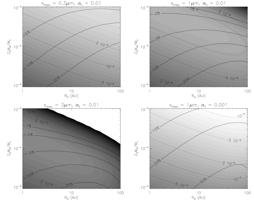
Figure 12: Heavy element retention of disks after total photo-evaporation of the gas as a function of the initial conditions of the disk, for various initial particle sizes and turbulent parameter $\alpha_{\rm t}$. The color scheme is the same for all four plots. The solid lines (at 1, 2, 5, 10, 20 and 50%) mark the retention efficiency, namely the percentage of heavy elements remaining in the disk compared with its initial content $Z_{0}M_{0}$. The dotted lines (at $10^{-6}$, $2\times 10^{-6}$, $5\times 10^{-6}$, $10^{-5}$, $2\times 10^{-5}$, $5\times 10^{-5}$, $10^{-4}$ and finally $2\times 10^{-4}M_{\star}$) follow the colored contours and mark the actual total mass of the remaining solids. Note that $1M_{\oplus}\simeq 3\times 10^{-6}M_{\odot}$ so that the $10^{-4}$ contour corresponds to about 33 $M_{\oplus}$.

Four cases are considered, with varying initial particle size $s_{\rm max0}$ and turbulent $\alpha_{\rm t}$. The weak dependence on the initial conditions of the disk ($M_{0}$, $R_{0}$) for given values of $\alpha_{\rm t}$ and $s_{\rm max0}$ suggested by equation (78) is naturally still present: it appears that even with $M_{0}$ and $R_{0}$ varying by two orders of magnitude, the remaining amount of solids does not vary more a factor of a few. In the fiducial model for instance ($s_{\rm max0}=1\mu$m and $\alpha_{\rm t}=0.01$) the typical amount of solids left is of the order of a few Earth masses for most plausible values of $M_{0}$ and $R_{0}$.

As suggested by the results of §5.3.2, the retention efficiency drops dramatically for larger initial grain sizes, but naturally saturates near the value given by equation (78) for very small grain sizes (e.g. compare the results for $s_{\rm max0}=3\mu$m with the results for $s_{\rm max0}=0.3\mu$m). Also suggested by (78) is the dependence of the phenomena on $\alpha_{\rm t}$: for the smaller value of $\alpha_{\rm t}=0.001$, one could expect up to a few tens of Earth masses to be left behind in the disk, a value that begins to be consistent with the amount of solids left in the Minimum Solar Nebula model augmented with the mass of the Oort cloud. Thus it appears that consistency of this idea with our own solar system would strongly favour a model with $s_{\rm max0}$ is no larger than $1\mu$m, and $\alpha_{\rm t}$ is preferably of the order of 0.001.

How reliable is this estimate given the simplifications made in the model? Conveniently, given that the total disk mass resides mostly in the outer disk, and that the amount of material remaining in the inner disk is ultimately controlled by the mass flux from the outer reservoir, the mass estimates given here are reasonably independent of the physics of the inner disk (including sublimation/condensation, but also dead zones, etc..). There is however an important caveat; as mentioned earlier, large protoplanetary embryos which have reached isolation mass are fully decoupled from the disk dynamics (both in terms of their drift velocity and in terms of their collision frequency), and are not well-modeled by the size distribution function proposed. The mass contained in these embryos could add a few Earth masses to what is presently estimated, but only in the inner disk. The total mass of solids which ends up being shepherded out to the outer solar system is not affected by this problem, and is therefore reliably estimated by this method.

7 Conclusions

This paper presents a new algorithm modeling the evolution of gas and solids in protostellar, as well as some reliable quantitative analytical estimates for the outcome of the numerical simulations.

The global disk evolution paradigm is well-reproduced by the numerical solutions. Well-known results are recovered, such as the two-timescale gas evolution (Clarke, Sotomayor & Gendrin 2001; Alexander, Clarke & Pringle 2006a), the rapid growth of solids in the inner disk (Suttner & Yorke, 2001, Stepinski & Valageas, 1997, Dullemond & Dominik, 2005), the shepherding of smaller particles by the retreating hole front (Alexander & Armitage 2007), and the accumulation of material near the sublimation lines (Stevenson & Lunine, 1988, Stepinski & Valageas 1997, Ciesla & Cuzzi, 2006).

Novel conclusions of this paper are:

(i) The evolution of the mass of solids in the disk is essentially controlled by a reservoir of small grains at large radii. A well-tested empirical formula for the total solid mass in the disk is given in equation (75).

(ii) The heavy-element retention efficiency after gas dispersal is controlled by the remaining amount of solids left at the time of gap opening, and is found to vary weakly with initial disk conditions but very sensitively with initial particle size $s_{\rm max0}$. The remaining amount of solids in the Minimum Solar Nebula combined with the mass of the Oort cloud is inconsistent with $s_{\rm max0}$ greater than 1$\mu$m, and would tend to prefer a value of $\alpha_{\rm t}\simeq 0.001$.

(iii) The strong dependence of the gas dispersal timescale on the initial mass and radius of the disk combined with the weak dependence of the heavy element retention efficiency on the same parameters could simultaneously explain the wide diversity of the SED observations with the very low dispersion of the stellar metallicities observed in the Pleiades (Wilden et al. 2002).

(iv) Rapid grain growth in the inner disk implies that solids in the form of large planetesimals (with sizes ranging from a few meters to 1000 km) are locally retained after gas dispersal. The presence of a population of large planetesimals in the inner regions of debris disks has been inferred from interferometric observations of the presence of dust despite its very short radiation blowout time (specifically in TW Hya, by Eisner, Chiang & Hillenbrand 2006)

(v) All the small grains are swept by the retreating gas front at the edge of the hole and shepeherded outward. When the accumulated surface density of grains approaches that of the gas, the gas becomes unable to continue moving the grains and will most likely leave them behind. This could explain the systematic formation of narrow dust rings at large radii.

(vi) Regulation of the solid mass flux by the “leaky reservoir” implies that any local surface density enhancement (or “peaks”) near sublimation lines must be accumulated very early on in the disk lifetime, more precisely during the initial phase when the disk dynamics are still out of equilibrium ($\sim$ first 10,000-100,000 yr). The gradual decay of the inner disk gas density through photo-evaporation could then trigger gravitational instabilities at well-separated times as each peak respectively approaches unit metallicity.

(vii) Possible constraints on the sticking efficiency of particles in the turbulent conditions found in protostellar disks could be derived from spatially resolved observations of the grain surface density of nearby disks (see Appendix C).

Direct comparison of the model predictions with disk SEDs is the subject of Paper II.

Acknowledgements: I thank Richard Alexander, Jeff Cuzzi, Tristan Guillot, Katherine Kretke, Francis Nimmo, Doug Lin and Andrew Youdin for pointing me in the right direction. I would have liked to acknowledge a funding source.

Appendix A: Photo-evaporation model

Alexander & Armitage (2007) studied the following model for the mass loss rate from photo-evaporation from the central star, based on the works of Hollenbach et al. (1994), Font et al. (2004), as well as Alexander, Clarke & Pringle (2006a and 2006b).

Prior to the removal of the gas in the inner disk, the mass loss rate is caused by the diffuse UV field reprocessed high in the disk atmosphere. It is equal to

$$\dot{\Sigma}_{\rm w}(r)=2n_{0}(r)u_{\rm l}(r)\mu m_{\rm H}\mbox{ , }$$ (1)

where $\mu$ is the mean molecular weight of the ionized gas (taken to be $\mu=1.35$), $m_{\rm H}=1.67\times 10^{-24}$g is the mass of the Hydrogen atom, the column density at the base of the ionized layer $n_{0}$ is taken to be (see Font et al. 2004)

$$n_{0}(r)=0.14\left(\frac{\Phi}{4\pi\alpha_{\rm B}R_{\rm g}^{3}}\right)^{1/2}\left[\frac{2}{(r/R_{\rm g})^{15/2}+(r/R_{\rm g})^{25/2}}\right]^{1/5}\mbox{ , }$$ (2)

with $\Phi$ is the photo-ionizing flux (in photons per second), $\alpha_{\rm B}=2.6\times 10^{-13}$cm³/s, $R_{\rm g}=GM_{*}/c_{i}^{2}$ and $c_{i}$ is the sound speed of the ionized gas (taken to be 10km/s in the fiducial model). The launch velocity $u_{\rm l}(r)$ is taken to be (see Font et al. 2004)

$$u_{\rm l}(r) = 0.3423c_{i}\exp\left[-0.3612\left(\frac{r}{R_{\rm g}}-1\right)\right]\left(\frac{r}{R_{\rm g}}-1\right)^{0.2457}\mbox{ if }r>0.1R_{\rm g}\mbox{ , }$$ (3)

$$= 0\mbox{ if }r<0.1R_{\rm g}\mbox{ . }$$

After clearing of the inner disk, the mass loss rate is mostly caused by direct photo-ionization of the inner edge of the remaining disk, and accordingly changes to

$$\dot{\Sigma}_{\rm w}(r,t)=0.47\mu m_{\rm H}c_{i}\left[1+\exp\left(-\frac{r-r_{\rm hole}(t)}{h(r_{\rm hole}(t))}\right)\right]^{-1}\left(\frac{\Phi}{4\pi\alpha_{\rm B}r^{3}_{\rm hole}(t)}\right)^{1/2}\left(\frac{h}{r}\right)^{-1/2}\left(\frac{r}{r_{\rm hole}(t)}\right)^{-2.42}\mbox{ , }$$ (4)

where $r_{\rm hole}(t)$ is the hole radius, well approximated to be the radius for which $\Sigma(r,t)$ drops below $10^{-7}$g/cm² (Alexander, private communication).

Appendix B: Numerical method

Equations (1), (7) (for each species), (36) or (44), and finally (46) (for each species) are evolved simultaneously in time using the following approach.

The independent variables $r$ and $t$ are first normalized to 1 AU and to $T_{\rm AU}=2\pi/\Omega_{\rm K}(1{\rm AU})$ respectively. Following Pringle, Verbunt & Wade (1986), a new variable is introduced

$$y=r_{\rm AU}^{1/2}\mbox{ , }$$ (5)

upon which space is uniformly discretized. Next, new dependent variables $G$, $G^{i}_{\rm v}$ and $G^{i}_{\rm p}$ are defined as

$$G=y^{2q+4}\Sigma\mbox{ and }G^{i}_{\rm v,p}=y^{2q+4}\Sigma^{i}_{\rm v,p}\mbox{ . }$$ (6)

With these modifications, equations (1) and (46) can be rewritten as

$$\frac{\partial G}{\partial t_{\rm AU}}=\frac{3\pi}{2}\alpha_{\rm t}\sqrt{\gamma}\overline{h}_{\rm AU}^{2}y^{2q+1}\frac{\partial^{2}G}{\partial y^{2}}-T_{\rm AU}y^{2q+4}\dot{\Sigma}_{\rm w}\mbox{ , }$$ (7)

(and similarly for each vapor-form species) where $t_{\rm AU}=t/T_{\rm AU}$. The evolution equation for the solids becomes

$$\frac{\partial G_{\rm p}^{i}}{\partial t_{\rm AU}} + y^{2q+1}\frac{\partial}{\partial y}\left[\left(\frac{\pi}{2}\alpha_{\rm t}\sqrt{\gamma}\overline{h}_{\rm AU}^{2}(Sc_{\rm eff}^{-1}-3I)\frac{\partial\ln G}{\partial y}-\frac{2\pi\eta J}{y^{2q+3}}\right)G_{\rm p}^{i}\right]$$ (8)

$$= \frac{\pi}{2}\alpha_{\rm t}\sqrt{\gamma}\overline{h}_{\rm AU}^{2}y^{2q+1}\frac{\partial}{\partial y}\left(\frac{1}{Sc_{\rm eff}}\frac{\partial G_{\rm p}^{i}}{\partial y}\right)\mbox{ , }$$

for each solid-form species. This formulation emphasizes the pure diffusive terms, which cause numerical instabilities if not treated adequately. For simplicity, $I\equiv I(\sqrt{2\pi St_{\rm max}})$ and similarly for $J$.

Equations (36) or (44) depending on the regime considered involve no spatial derivative, and are therefore simply integrated forward in time using a simple explicit second-order Adams-Bashforth scheme. Equations (8) and (7) are integrated forward in time using a centered implicit scheme for the diffusion terms, an upwind first-order scheme for the advection terms and a second-order Adams-Bashforth scheme for all other terms. With this particular semi-implicit scheme, it is found that using about 1000-4000 meshpoints (depending on the radial resolution required) and a typical timesteps $\Delta t\simeq 0.1-10$yr yields a stable and accurate solution.

Appendix C: A quick-and-dirty estimate for $\Sigma_{\rm p}(r,t)$

To get an estimate for $\Sigma_{\rm p}(r,t)$, one could use equation (50) together with equation (76). Unfortunately, the value of $St_{\rm max}(r,t)$ is unknown since it depends both on $s_{\rm max}(r,t)$ and on $\Sigma(r,t)$, neither of which are particularly well approximated in inner and intermediate regions of the disk. Nonetheless, let’s construct a low-quality estimate of $St_{\rm max}(r,t)$ using the following algorithm: at each radius $r$ and time $t$,

$$s_{\rm max}(r,t) := \max\left[\frac{\sqrt{2\pi\gamma}}{\rho_{\rm s}}\left(\frac{t}{{\rm 1year}}\right)^{2}Z_{0}^{2}\epsilon^{2}\alpha_{t}\Sigma(r,t)r_{\rm AU}^{-3}\left(\frac{M_{\star}}{M_{\odot}}\right),s_{\rm max0}\right]\mbox{ , }$$

$$m_{\rm iso}(r,t) := \left[2\pi r^{2}Z_{0}\Sigma(r,t)\tilde{b}\left(\frac{2}{3M_{\star}}\right)^{1/3}\right]^{3/2}\mbox{ , }$$

$$s_{\rm max}(r,t) := \min\left[s_{\rm max}(r,t),\left(\frac{3m_{\rm iso}(r,t)}{4\pi\rho_{\rm s}}\right)^{1/3}\right]\mbox{ , }$$

$$St_{\rm max}(r,t) := \frac{s_{\rm max}(r,t)\rho_{\rm s}}{\sqrt{2\pi\gamma}\Sigma(r,t)}\mbox{ , }$$ (9)

where $m_{\rm iso}(r,t)$ is an estimate of the local isolation mass, and where $\Sigma(r,t)$ is given by the self-similar solution (55). The resulting predicted solution for $\Sigma_{\rm p}(r,t)$ is shown in Figure 13 at $t=4.5$Myr, for the three initial particles sizes considered in the text (1, 3 and 10$\mu$m). While the global features of the solution are fairly well reproduced, the quantitative predictions are clearly off by up to an order of magnitude in regions I and II of the disk, and even larger in region III where equation (76) looses validity.

Figure 13: True numerical solution (solid lines) and approximate estimates for the total surface density of solids, using the algorithm shown in Appendix C. The estimate for 1$\mu$m size particles is shown as a dotted line, 3$\mu$m as dot-dash line and 10$\mu$m as a dashed line. Note that some of the global trends (in particular the overall normalization of the curve, and the surface density dip) are well-reproduced by the estimate but that quantitative agreement is poor.

Note that one of the features that is well-reproduced by the solution is the sharp decrease in the surface density of particles in the intermediate regions of the disk. This feature corresponds to radii where $St_{\rm max}\simeq 1$, which is approximately where

$$r_{\rm dip}=4.64\left(\frac{Z_{0}}{0.01}\right)^{2/3}\left(\frac{\epsilon}{0.01}\right)^{2/3}\left(\frac{\alpha_{\rm t}}{0.01}\right)^{1/3}\left(\frac{M_{\star}}{M_{\odot}}\right)^{1/3}\left(\frac{t}{1{\rm Myr}}\right)^{2/3}{\rm AU}\mbox{ . }$$ (10)

Interestingly, $r_{\rm dip}$ is entirely independent on the initial conditions of the disk ($M_{0}$ and $R_{0}$). Since $Z_{0}$, $M_{\star}$ and $t$ should be fairly well observationally determined by the stellar properties, possible measurements of $r_{\rm dip}$ may help constrain the product $\epsilon^{2}\alpha_{\rm t}$ (at least within an order of magnitude).

References

- (1) Alexander, R. D., Clarke, C. J. & Pringle, J. E., 2006a, MNRAS, 369, 216
- (2) Alexander, R. D., Clarke, C. J. & Pringle, J. E., 2006b, MNRAS, 369, 229
- (3) Alexander, R. D. & Armitage, P. J., 2007, MNRAS, 375, 500
- (4) Apai, D. et al. 2005, Science, 310, 834
- (5) Carballido, A., Fromang, S. & Papaloizou, J., 2006, MNRAS, 373, 1633
- (6) Clarke, C. J., Gendrin, A., & Sotomayor, M. 2001, MNRAS, 328, 485
- (7) Ciesla, F.J., & Cuzzi, J.N., 2006, Icarus, 181, 178
- (8) Dubrulle, B., Morfill, G. & Sterzik, M., Icarus, 114, 237
- (9) Dullemond, C.P., & Dominik, C. 2005, å, 434, 971
- (10) Dullemond, C.P., Hollenbach, D., & Kamp, I., & D’Alessio, P. 2006, in Protostars & planets V
- (11) Dominik, C., Blum, J., Cuzzi, J.N. & Wurm, G., 2007, in Protostars & Planets V
- (12) Eisner, J. A., Chiang, E.I., & Hillenbrand, L.A., 2006, ApJ, 637, L133
- (13) Fischer, D. A. & Valenti, J., 2005, ApJ, 622, 1102
- (14) Font, A. S., McCarthy, I. G., Johnstone, D., & Ballantyne, D. R., 2004, ApJ, 607, 890
- (15) Fromang, S. & Nelson, R. P., 2006, å, 457, 343
- (16) Gammie, C.F. 1996, ApJ, 457, 355
- (17) Garaud P., Barrière-Fouchet, L. & Lin D.N.C. 2004, ApJ, 603, 292
- (18) Garaud P., & Lin D.N.C. 2007, ApJ, 654, 606
- (19) Guillot, T. et al. 2006, å, 453, L21
- (20) Haisch, K. E. Jr., Lada, E. A. & Lada, C. J. 2001, ApJ, 553, 153
- (21) Hartmann, L., Hewett, R. & Calvet, N. 1994, ApJ, 426, 669
- (22) Hartmann, L., Calvet, N., Gullbring, E. & D’Alessio, P., 1998, 495, 385
- (23) Hartmann, L. et al. 2005, ApJ, 629, 881
- (24) Hollenbach, D., Johnstone, D., Lizano, S. & Shu, F., 1994, ApJ, 428, 654
- (25) Hollenbach, D. & Gorti, U., 2005, in Protostars and planets IV
- (26) Hueso, R. & Guillot, T., 2005, å, 442, 703
- (27) Kokubo, E., Ida, S. 2002, ApJ, 581, 666
- (28) Liffman, K., 1998, PASA, 20, L337
- (29) Lynden-Bell, D., & Pringle, J.E., 1974, MNRAS, 168, 603
- (30) Mamajek, E. E. et al. 2004, ApJ, 612, 496
- (31) Mathis J. S., Rumpl W., & Nordsieck K. H., 1977, ApJ, 217, 425
- (32) Meeus, G., Sterzik, M. Bouwman, J. & Natta, A., 2003, å, 409, L25
- (33) Morfill, G.E., & Voelk, H.J., 1984, ApJ, 287, 371
- (34) O’Brien, D. P. & Greenberg, R., 2003, Icarus, 164, 334
- (35) Ormel, C. W. & Cuzzi, J. N. 2007, å, 466, 413
- (36) Pollack, J. B. et al. 1994, ApJ, 421, 615
- (37) Ruden, S. P., 2004, ApJ, 605, 880
- (38) Schneider, G. et al. 2006, ApJ, 650, 414
- (39) Sicilia-Aquilar, A. et al., 2006, ApJ, 638, 897
- (40) Stepinski, T. F. & Valageas, P., 1997, å, 319, 1007
- (41) Stevenson, D. J., & Lunine, J. I., 1988, Icarus, 75, 146
- (42) Strubbe, L. E. & Chiang, E. I., 2006, ApJ, 648, 652
- (43) Suttner, G. & Yorke, H. W., 2001, ApJ, 551, 461
- (44) Takeuchi, T., Clarke, C. & Lin, D. N. C., 2005, ApJ, 627, 286
- (45) Turner, N. J., Sano, T., & Dziourkevitch, N., 2007, ApJ, 659, 729
- (46) Voelk, H. J., Jones, F. C., Morfill, G. E. & Roeser, S., 1980, å, 85, 316
- (47) Weidenschilling S. J., 1977, MNRAS, 180, 57
- (48) Weidenschilling, S.J. 1984, Icarus, 60, 553
- (49) Weidenschilling S. J., & Cuzzi, J. N., 1993, Protostars & Planets III, 1031
- (50) Wilden, B.S., Jones, B.F., Lin, D.N.C., & Soderblom, D.R. 2002, AJ, 124, 2799
- (51) Whipple F. L., 1972,From plasma to planet, ed. A. Elvius, Wiley, London