Weak first-order transition in the three-dimensional site-diluted Ising antiferromagnet in a magnetic field

Abstract

We perform intensive numerical simulations of the three-dimensional site-diluted Ising antiferromagnet in a magnetic field at high values of the external applied field. Even if data for small lattice sizes are compatible with second-order criticality, the critical behavior of the system shows a crossover from second-order to first-order behavior for large system sizes, where signals of latent heat appear. We propose “apparent” critical exponents for the dependence of some observables with the lattice size for a generic (disordered) first-order phase transition.

I INTRODUCTION

The study of systems with random fields is of paramount importance in the arena of the disordered systems. A paradigm in this field is the random field Ising model belanger ; nattermann (RFIM). In spite of much effort devoted to the investigation of the RFIM, nattermann several important questions remain open. Some of these questions refer to the nature of the (replica symmetric?) low temperature phase, to universality issues (binary versus Gaussian external magnetic field sourlas ; parisi-sourlas ), and to the order of the phase transitions. Here we study the diluted antiferromagnetic Ising model in an external magnetic field (DAFF) that is believed to belong to the same universality class of the RFIM (the DAFF is expected to behave as a Gaussian RFIM because of the short ranged correlations in the superexchange coupling). aharony_II ; cardy

As a matter of fact, DAFF systems are the most widely investigated experimental realization of the RFIM. One of the best examples of a diluted Ising antiferromagnet is $\mathrm{Fe}_{x}\mathrm{Zn}_{1-x}\mathrm{F}_{2}$. Its large crystal field anisotropy persists even when the $\mathrm{Fe}$ ions are diluted ($x<1$), thus providing a good (antiferromagnetic) Ising system for all ranges of the magnetic concentration. Other systems behaving as Ising (anti)ferromagnets are $\mathrm{Fe}_{x}\mathrm{Mg}_{1-x}\mathrm{Cl}_{2}$, $\mathrm{Co}\mathrm{Zn}_{1-x}\mathrm{F}_{2}$ and $\mathrm{Mn}_{x}\mathrm{Zn}_{1-x}\mathrm{F}_{2}$. belanger The experimental results on the order of the phase transition are somewhat inconclusive. On the one hand, these materials show a large critical slowing down around the critical temperature, as well as a symmetric logarithmic divergence of the specific heat. On the other hand, the order parameter (the staggered magnetization) behaves with a critical exponent $\beta$ near zero, possibly marking the onset of a first-order phase transition. belanger Note that $\beta$ should be exactly zero if the order parameter is discontinuous as a function of temperature or the magnetic field.

The numerical investigations of the DAFF at $T>0$ are scarce. It was investigated a long time ago by Ogielski and Huse. ogielski They considered several values of the pair temperature–magnetic field on lattice sizes up to $L=32$ but far from the critical region. fn1 They investigated the thermodynamics as well as the (equilibrium) dynamical critical behavior. Their thermodynamic results pointed to a second-order phase transition. However, they found activated dynamics (which could be interpreted as a signal of a first-order phase transition) rather than standard critical slowing down (for numerical studies of the DAFF at $T=0$, see Refs. [sourlas, ] and [hartmann1, ]).

Numerical and analytical studies rather focused on the RFIM, which is expected to display the DAFF critical behavior. aharony_II ; cardy Even if the RFIM is more amenable than the DAFF to analytical investigations, the situation is still confusing. Indeed, mean-field theory predicts a second-order phase transition for low magnetic field. If the probability distribution function of the random fields does not have a minimum at zero field, the transition is expected to remain of the second-order all the way down to zero temperature. However, if the probability distribution for the random field does show a minimum at zero field, a tricritical point and a first-order transition line at sufficiently high field values are predicted. aharony_I

The numerical investigation of the RFIM has neither confirmed nor refuted this counterintuitive mean-field result. Rieger and Young studied binary distributed quenched magnetic fields, rieger_II where mean-field predicts a tricritical point. After extrapolation to the thermodynamic limit, they interpreted their results as indicative of a first-order transition for all external field strengths in the thermodynamic limit (the tricritical point did not show up). Rieger studied the case with Gaussian fields, rieger_I where only second-order behavior should be found according to mean-field expectations. Actually, his results were consistent with a second-order phase transition with vanishing (!) order parameter exponent. The simulation of Hernandez and Diep hernandez of the binary RFIM supports the existence of a tricritical point at finite temperature and magnetic field. Also the study by Machta et al. Machta of the Gaussian RFIM showed evidences of finite jumps in the magnetization at disorder dependent transition points.

A completely different numerical strategy is suggested by the expectations of a $T\!=\!0$ renormalization-group fixed point BRAYMOORE . Since the ground state for a RFIM on a sample of linear size $L$ can be found in polynomial (in $L$) time, $T\!=\!0$ physics can be directly addressed by studying the properties of the ground state for a large number of samples. Hartmann and Young hartmann2 studied lattices up to $L\!=\!96$ for the gaussian RFIM. They concluded that their data supported a second-order phase transition scenario for the Gaussian RFIM. The same model was investigated by Middleton and Fisher middleton in lattices up to $L\!=\!256$. Their data suggested as well a continous phase transition with a very small order parameter exponent, $\beta\!=\!0.017(5)$. Using the same technique Hartmann and Nowak hartmann1 found non-universal behavior in the binary and Gaussian RFIM, not excluding that the former could undergo a first-order phase transition. They also studied $T\!=\!0$ critical properties of the DAFF for system sizes up to $L\!=\!120$, and found critical exponents $\beta\!=\!0.02(1)$, $\nu\!=\!1.14(10)$ and $\overline{\gamma}\!=\!3.4(4)$, compatible with their results for the Gaussian RFIM.

The aim of this work is to revisit the Ogielski-Huse investigation, that was carried out for $T>0$, with modern computers, algorithms pt and finite-size scaling methods (the quotient method, quotient that uses the finite volume correlation length cooper to characterize the phase transition). The significant CPU investment allowed us to simulate large lattices ($L\!=\!24$) and a large number of disorder realizations. We plan, in the future, to perform a more complete investigation of the critical surface of this model (this would require to vary three variables: temperature, dilution and magnetic field).

Our main finding is that the DAFF probably undergoes a very weak first-order phase transition. This seems a natural explanation for the finding of the activated dynamics (at equilibrium) in Ref. [ogielski, ]. The discontinuity in the magnetization density is sizable, yet that of the internal energy is very small. Nevertheless, even if we perform a standard second-order analysis, the critical exponent for the staggered magnetization turns out to be ridiculously small.

The outline of the rest of this paper is the following: in the next section we describe the model (Sect. II.1), observables (Sect. II.2), as well as the theoretical expectations for the finite-size scaling behavior in a second-order phase transition (Sect. II.3) and for a first-order one (Sect. II.4). Details about our simulations are given in Sect. III. Our numerical results are presented in Sect. IV. We first perform a second-order analysis (Sect. IV.1), then consider the possibility of a weak first-order transition (Sect. IV.2). After summarizing our results in Sect. V, we discuss in the Appendix that the bound chayes $\nu\geq 2/d$ of Chayes et al. holds as well for first-order phase transitions in the presence of disorder. In addition, we have found upper bounds for the divergence of the susceptibility and specific heat with the lattice size.

II Model

II.1 Model, phase diagram, symmetries

The model is defined in terms of Ising spin variables $S_{i}=\pm 1$, $i=1,\dots,V=L^{3}$ placed on the nodes of a cubic lattice of size $L$ with periodic boundary condition. The spins interact through the following lattice Hamiltonian

$$\mathcal{H}=\sum_{<i,j>}\epsilon_{i}S_{i}\epsilon_{j}S_{j}-H\sum_{i}\epsilon_{i}S_{i}\,,$$ (1)

where the first sum runs over pairs of nearest-neighbor sites, while $H$ is the external uniform magnetic field. The $\epsilon_{i}$ are quenched dilution variables, taking values $0$ and $1$ (with probability $1-p$ and $p$ respectively) in empty and occupied sites. In this work we have fixed this probability to $p=0.7$. In this way we are guaranteed to stay away from both from the pure case ($p=1$) and the percolation threshold ($p_{c}\approx 0.31$). stauffer

It is understood that for every choice of the $\{\epsilon_{i}\}_{i=1}^{V}$, called hereafter a sample or a disorder realization, we are to perform the Boltzmann (thermal) average. The mean over the disorder is only taken afterwards.

For low magnetic field, at low temperatures, model (1) stays in an antiferromagnetic state that we will call the ordered phase. The staggered magnetization $M_{\mathrm{s}}$, see Eq.(2) below, is an order parameter for this phase. Note that, for $H=0$, the $Z_{2}$ transformation $S_{i}\rightarrow-S_{i}$, yields a degenerate antiferromagnetic state. The increase of the magnetic field or the temperature $T$ weakens the antiferromagnetic correlations, and the system eventually enters into a paramagnetic state. The paramagnetic and the ordered phases are separated by a critical line in the ($T$,$H$) plane [it would be a critical surface in the ($T$,$H$,$p$) phase diagram].

Note that the effect of disorder (quenched dilution), combined with the applied field $H$ in a finite DAFF system, breaks the $Z_{2}$ symmetry even in the ordered phase. Consider the state of minimal energy at $T=0$ and $H$ low enough so that the staggered magnetization is maximal and $M_{\mathrm{s}}=p$. Now let us change the sign to all spins in one hit: if $p=1$, the two states are completely degenerate, but the random dilution introduces a subextensive shift in the total energy. In fact, the inversion does not change the nearest-neighbor energy, but changes the sign of the magnetic part. In the pure system the magnetic energy of the fully ordered antiferromagnetic state is zero but, in the presence of random dilution, the number of spins aligned or misaligned with the field $H$ is a random variable. So, the total magnetic contribution to energy is of order $\left[p(1-p)N\right]^{1/2}$. It follows that the $M_{\mathrm{s}}=-p$ state has an energy shift of order $2\left[p(1-p)N\right]^{1/2}$ with respect to the $M_{\mathrm{s}}=p$ one and its Boltzmann weight is depressed (an analogous effect of degeneration removal is present in the RFIM). A “quasisymmetric” state may exist if there is a configuration of spins in which almost all the spins are reversed with respect to the $M_{s}=p$ state such that the sum of the energies of unsatisfied bonds cancels the magnetic excess. If this is the case, then the two states are degenerate but the probability distribution of the order parameter results peaked around asymmetric values. The magnetic energy excess is a subextensive effect and is expected to be suppressed as $L$ increases. Nevertheless, the probability of transitions between states of opposite spontaneous staggered magnetizations decreases for large system, which is a major problem for simulations.

II.2 Observables

In the following, $\langle(\cdot\cdot\cdot)\rangle$ denotes thermal averages (including averages of real replicas) and $\overline{(\cdot\cdot\cdot)}$ indicates a sample average (average on the disorder). Measures focused on several observables: the order parameter, i.e., the average value of the staggered magnetization

$$\overline{\langle M_{\mathrm{s}}\rangle}=\frac{1}{V}\overline{\langle\sum_{j}\epsilon_{j}S_{j}e^{i\pi(\sum_{\mu=1}^{d}j_{\mu})}\rangle}\,,$$ (2)

($j_{\mu}$ is the $\mu$-th lattice coordinate of site $j$) whose values are limited in the interval $-p\leq M_{\mathrm{s}}\leq p$ (in average for large lattices); the average energy densities are

$$\frac{1}{V}\overline{\langle\mathcal{H}\rangle} = \overline{\langle E\rangle}=\overline{\langle E_{\mathrm{K}}\rangle}+H\overline{\langle E_{\mathrm{M}}\rangle}\,,$$ (3)

$$\frac{1}{V}\overline{\langle\mathcal{H}_{\mathrm{K}}\rangle} = \overline{\langle E_{\mathrm{K}}\rangle}=\frac{1}{V}\overline{\langle\sum_{<i,j>}\epsilon_{i}S_{i}\epsilon_{j}S_{j}\rangle}\,,$$ (4)

$$\frac{1}{V}\overline{\langle\mathcal{H}_{\mathrm{M}}\rangle} = \overline{\langle E_{\mathrm{M}}\rangle}=-\frac{1}{V}\overline{\langle\sum_{i}\epsilon_{i}S_{i}\rangle}\,,$$ (5)

with $\mathcal{H}_{\mathrm{K}}$ and $\mathcal{H}_{\mathrm{M}}$ respectively the kinetic and magnetic contributions to the Hamiltonian. The definition of $E_{\mathrm{M}}$ coincides with the definition of the usual magnetization density.

We also computed the average values of the squares and fourth powers of the above quantities, and some cumulants and susceptibilities: given an observable $\frac{1}{V}\mathcal{A}=A$ we compute the Binder cumulant:

$$g_{4}^{A}=\frac{1}{2}\left(3-\frac{\overline{\langle A^{4}\rangle}}{\overline{{\langle A^{2}\rangle}}^{2}}\right)$$ (6)

and the connected and disconnected susceptibilities

$$\chi_{\mathrm{c}}^{A} = V\overline{\langle A^{2}\rangle-{\langle A\rangle}^{2}}\,,$$ (7)

$$\chi_{\mathrm{dis}}^{A} = V\overline{{\langle A\rangle}^{2}}\,.$$ (8)

These are the ordinary susceptibilities in case $A=M_{\mathrm{s}}$, while $\chi_{\mathrm{c}}^{\mathcal{H}}$ is proportional to the specific heat $C_{v}$.

The lack of $Z_{2}$ symmetry, explained in Sec. II.1 makes mandatory the use of connected correlation functions in finite lattice sizes, especially in the case of the order parameter $M_{\mathrm{s}}$. Yet, the connected staggered susceptibility $\chi_{\mathrm{c}}^{M_{\mathrm{s}}}=V\overline{\langle{M_{\mathrm{s}}}^{2}\rangle-{\langle{M_{\mathrm{s}}}\rangle}^{2}}$ does not show a peak in the $(T,H)$ ranges we considered, so we also study the behavior of the connected and disconnected staggered susceptibilities defined with the absolute value of the staggered magnetization:

$$\chi_{\mathrm{c}} = V\overline{\langle M_{\mathrm{s}}^{2}\rangle-{\langle\left|M_{\mathrm{s}}\right|\rangle}^{2}}\,,$$ (9)

$$\chi_{\mathrm{dis}} = V\overline{{\langle\left|M_{\mathrm{s}}\right|\rangle}^{2}}\,.$$ (10)

In the following, when no observable subscript is specified in the susceptibility symbol, we will be referring to Eqs. (9) and (10).

It will turn out useful to define a correlation length on a finite lattice by the following analogy with a (lattice) Gaussian model:cooper

$$\xi^{2}=\frac{G(k_{1})-G(k_{2})}{k_{2}^{2}G(k_{2})-k_{1}^{2}G(k_{1})}\,,$$ (11)

with $k^{2}=4\sum_{\mu=1}^{d}\sin^{2}{(k_{\mu}/2)}$ on a discrete lattice and $G(k)$ the momentum-dependent propagator

$$G(k) = V\overline{\langle F(k)F(-k)\rangle-\langle F(k)\rangle\langle F(-k)\rangle}\,,$$

$$= \frac{G_{0}}{\xi^{-2}+k^{2}}\ \ (k^{2}\ll\xi^{-2})\,,$$

$$F(k) = \frac{1}{V}\sum_{j}\epsilon_{j}S_{j}e^{i\sum_{\mu=1}^{d}(k_{\mu}+\pi)j_{\mu}}\,,$$ (13)

$$(G(0) = \chi_{c}^{M_{s}},\ F(0)=M_{s})\,,$$

and $F(k)$ the staggered Fourier transform of the spin field. Also in this case we use the connected part for $G(k)$. Choosing $k_{1}=(0,0,0)$ and $k_{2}=(2\pi/L)\hat{k}_{\mu}$ as one of the minimum wave vectors ($\hat{k}_{\mu},\ \mu=1,\dots,d$ are the $d$ versors in the reciprocal space), we have

$$\xi^{2}=\frac{1}{4\sin^{2}(\pi/L)}\left(\frac{\chi_{c}^{M_{s}}}{\left[\sum_{\mu=1}^{d}G\left({(2\pi/L)\hat{k}_{\mu}}\right)\right]/d}\right)\ \ .$$ (14)

Equation (14) is a good estimate of the correlation length only in the disordered phase but is useful to identify the critical region where $\xi/L$ should be a nontrivial universal value.

Finally, with mass storage not being a problem on modern equipment, it is easy to compute derivatives with respect to inverse temperature $\beta=1/T$ and applied field $H$, through connected correlations. In particular, the specific heat is

$$C_{v}=\frac{1}{V}\overline{\frac{d\langle\mathcal{H}\rangle}{dT}}\ \ \ .$$ (15)

II.3 Finite-size scaling in second-order phase transitions

We made use of finite size scaling, barber both studying the behavior of peaks of susceptibilities and applying the quotient method (QM) quotient to extract values for critical exponents. Let us briefly recall both.

Consider an observable $A$, that in the infinite volume limit behaves as $(T-T_{c})^{-a}=t^{-a}$ near the critical region ($t$ is the reduced temperature). Then, disregarding correction-to-scaling terms, we expect the following temperature dependency on a finite lattice of size $L$

$$A(L,t)=L^{a/\nu}f_{A}(tL^{1/\nu})\,,$$ (16)

with $\nu$ the correlation length exponent, $\xi\propto t^{-\nu}$, and $f_{A}(s)$ a smooth universal scaling function showing a peak at some value $s_{m}=t_{m}(L)L^{1/\nu}$. It follows that $T_{m}(L)-T_{c}^{\infty}\propto L^{-1/\nu}$. In addition, the scaling of the peak-height gives the value of the critical exponent $a$.

The QM is based on the same scaling ansatz:

$$A(L,t)=L^{a/\nu}g_{A}(\xi^{-1}(L,t)L)$$ (17)

We compare data in two lattices $L_{1}$ and $L_{2}$ at the (unique) reduced temperature $t^{*}$ where the correlation-length in units of the lattice size coincides, $\xi(L_{1},t)/L_{1}=\xi(L_{2},t)/L_{2}$. At this temperature we have, apart from corrections to scaling:

$$\frac{A(L_{1},t^{*})}{A(L_{2},t^{*})}=\left(\frac{L_{1}}{L_{2}}\right)^{a/\nu}$$ (18)

Note that the crossing temperature $T^{*}(L_{1};L_{2})$ approaches the critical temperature for large $L$ much faster than the peak of any susceptibility: $t^{*}=T^{*}(L_{1};L_{2})-T_{c}^{\infty}\propto L^{-\omega-1/\nu}$ ($\omega$ is the leading correction-to-scaling exponent).

From the definition [Eq. (14)] of the correlation length, one sees that, respectively, $\xi/L\sim O(L^{cd})$ in the “ordered” (low $T$, low $H$) phase and $\xi/L\sim O(1/L)$ in the “disordered” phase. The constant $c$ is $1/2$ in the case when the ordered phase has a $Z_{2}$ global symmetry, for in finite lattices the disconnected susceptibility would vanish. Near a second-order transition, $\xi/L$ does not depend on $L$, so there is a region in which $\xi/L$ for different lattice sizes cross each other. The method then consist in finding the value $T^{*}(L_{1};L_{2})$ at which this crossing happens and extracting the exponent $a/\nu$ by means of Eq. (18).

We apply the methods to several observables to extract exponents, in particular

$$\chi_{\mathrm{c}}^{M_{\mathrm{s}}},\chi_{\mathrm{c}} \longrightarrow a=\gamma=\nu(2-\eta)\,,$$ (19)

$$\chi_{\mathrm{dis}}^{M_{\mathrm{s}}},\chi_{\mathrm{dis}} \longrightarrow a=\overline{\gamma}=\nu(2-\overline{\eta})\,,$$ (20)

$$C_{v} \longrightarrow a=\alpha\,,$$ (21)

$$\left|M_{\mathrm{s}}\right| \longrightarrow a=-\beta\,,$$ (22)

$$\partial_{\beta}\xi \longrightarrow a=1+\nu\,.$$ (23)

Notice that we follow Ogielski and Huse ogielski in defining $\overline{\eta}$.

II.4 Finite-size scaling for first-order phase transitions

Finite-size effects in first-order phase transitions on pure systems are qualitatively similar to their second-order counterpart, provided that one considers effective critical exponents. binder_rev ; binlau_I ; binlau_II With the assumption that the lattice size is much larger than the correlation length, simple scaling relations hold for the size of the broadened transition region, the height of the peak of the specific heat and the extremal point of the binder cumulant for the energy density: denoting with subscripts $+$ and $-$ values of observables of the two competing phases at a first-order transition in the infinite volume limit (one of the phases can be degenerate) and being $Q=E_{+}-E_{-}$ the latent heat, one has the following in a finite system: binlau_II

$$T^{*}(L)-T_{c} = a(Q)L^{-d}\,,$$ (24)

$$C_{v}(T^{*}) = c_{1}(C_{v+},C_{v-})+c_{2}(Q)L^{d}\,,$$ (25)

$$1-g_{4}^{E}(T^{*}) = g_{1}(E_{+},E_{-})$$

$$+ g_{2}(E_{+},E_{-},C_{v+},C_{v-})L^{-d}\,,$$

where, in particular, $a(Q)$, $c_{2}(Q)$ and $g_{1}(E_{+},E_{-})$ vanish if the latent heat is zero, i.e., $E{+}=E_{-}$. $C_{v\pm}$ are the specific heats of the $\pm$ phases. Finally, the susceptibility also diverges with the volume of the system.

However, in the presence of disorder the scaling law of $T^{*}(L)-T_{c}$ should be modified (see the appendix)

$$T^{*}(L)-T_{c}=b(Q)L^{-d/2}\,.$$ (27)

This follows, for instance, from a simple mean-field argument, Chatelain01 that yields a linear relation between the critical temperature and the number of spins in the samples. Since the average spin density fluctuates as $L^{-d/2}$, we expect this to be the width of the critical region on finite lattices. Furthermore, the specific heat and the connected susceptibility may diverge only as fast as $L^{d/2}$. See the appendix for a detailed discussion of these bounds.

Hence, assuming that the observables diverge as much as possible, we can write the following “apparent” critical exponents for a disordered first-order transition:

$$\frac{1}{\nu}=\frac{d}{2}\ ,$$ (28)

$$\frac{\alpha}{\nu}=\frac{d}{2}\ ,$$ (29)

$$\frac{\gamma}{\nu}=\frac{d}{2}\ .$$ (30)

From the last equation and using $\eta=2-\gamma/\nu=2-d/2$, we find in $d=3$ that $\eta=0.5$ and $\nu=2/3$.

If we assume that the averaged probability distribution of the energy $\overline{\langle P(E)\rangle}$ is composed (in the thermodynamic limit and at the critical point) bof the sum of Dirac deltas, we should obtain a divergence $L^{d}$ for the normalized variance of this averaged probability, obtaining (e.g., for the energy)

$$L^{d}\left(\overline{\langle E^{2}\rangle}-\overline{\langle E\rangle}^{2}\right)=Q^{2}L^{d}\,.$$ (31)

In particular, we should recover Eq. (II.4) for $g_{4}^{E}$ which is computed with $\overline{\langle P(E)\rangle}$ [see Eq. (6)]. Please note that the width of $\overline{\langle P(E)\rangle}$ is not related to the specific heat, which is rather related to $L^{d}\left(\overline{\langle E^{2}\rangle}-\overline{\langle E\rangle^{2}}\right)$.

Figure 1: The connected susceptibility computed with $\left|M_{s}\right|$ as function of $T$ for lattice sizes $L=8,12,16,20$ and $24$. Lines are interpolating splines as a guide to the eye.

Figure 2: Top: the susceptibility peak height as function of $L^{\gamma/\nu}$. Bottom: Peak position as function of $L^{-1/\nu}$. Solid lines are the fitting power-law functions. See section IV.1 for more details.

III Simulation details

We simulate the model using the usual Metropolis algorithm with sequential spin flip schedule and the parallel tempering technique. pt We restricted our simulation to the

$$H=1.5T$$ (32)

diagonal in the $(T,H)$ plane in order to keep away from the crossover to the zero field case. This should also avoid problems with an oblique crossing of the transition line and will help in the comparison with previous numerical simulations. ogielski

The critical temperature on this diagonal stays around $T_{c}=1.5$, and we simulated $N_{T}=29$ temperatures for every lattice size at equally spaced $(T,H)$ values along this diagonal. For smaller lattices ($L=8,\ 12,$ and $16$) the $T$ values were in the range $[1.3,2.7]$, while for the larger sizes ($L=20$ and $24$) the temperature range was $[1.3,2.0]$. For every lattice size, $1280$ samples (different realizations of the disorder) were simulated. Statistics is also doubled as our program processes two real replicas per sample, with the same disorder, at each $(T,H)$ value.

$L$	$N_{\mathrm{samples}}$	$N_{T}$	$t_{\mathrm{sim}}$	$T_{\mathrm{max}}$	$T_{\mathrm{min}}$
$8$	$1280$	$29$	$2\times 10^{6}$	$2.7$	$1.3$
$12$	$1280$	$29$	$2\times 10^{6}$	$2.7$	$1.3$
$16$	$1280$	$29$	$8\times 10^{6}$	$2.7$	$1.3$
$20$	$1280$	$29$	$1.6\times 10^{7}$	$2.0$	$1.3$
$24$	$1280$	$29$	$2.4\times 10^{7}$	$2.0$	$1.3$

Table 1: Parameters characterizing the simulation. See text for details.

The use of optimized asynchronous multispin coded update routines in our programs allowed us to thermalize systems on lattices with size up to $L=24$. The program can perform Metropolis update at a $1.3~{}\mbox{ns}/\mbox{spin}$ rate on a conventional $64$ bits Intel CPU at 3.4 GHz. Of course, the use of parallel tempering (PT) slows down the performance of the multispin code simulation, but we can limit the loss of performance if we let the program perform PT swaps every many Metropolis lattice sweeps. We verified that a PT swap trial every 20 Metropolis lattice sweeps also allows for hotter replicas to decorrelate before the exchange with colder ones, at the cost of a factor of $1.5$ in performances. Cluster update algorithms did not prove convenient due to a dramatic increase in total computational load. In what follows, we consider simulation time units such that $20$ Monte Carlo (MC) steps are $20$ Metropolis full lattice updates plus $1$ PT step.

Simulating $1280$ samples for the largest lattice ($L=24$ and $24\times 10^{6}$ MC steps) took about four weeks and 20 computation nodes on the Linux cluster at BIFI. By monitoring nonlocal observables (like the susceptibilities), we have checked that the runs are thermalized: we have reached a plateau in all the nonlocal observables we are measuring. In particular, for each lattice size, let $t_{\mathrm{sim}}$ be the total time in MC steps devoted to simulate a sample, the time needed to achieve equilibrium always resulted shorter than $t_{\mathrm{sim}}/2$. Indeed, we discarded measures at all times $t<t_{\mathrm{sim}}/2$. Simulation parameters are summarized in Table 1.

Two further thermalization test were provided by the parallel tempering statistics: (1) we have checked that the temperature samples perform all the road from higher to lower temperatures and come back; (2) the temperature samples have stayed essentially the same Monte Carlo time in all the temperatures simulated.

IV NUMERICAL RESULTS

IV.1 Second-order phase transition scenario

We will use first the old fashioned peak method and turn later to the quotient method. In this way we will obtain complementary information.

In Fig. 1 we show the staggered magnetization connected susceptibility $\chi_{\mathrm{c}}$ data. Clear peaks are present from which it is possible to extract information on exponents $\gamma$, $\nu$ and $\eta$. There is a lot of noise in the signal for $\chi_{\mathrm{c}}$ at low temperatures for large lattice sizes ($L=20$ and $L=24$). This is almost exclusively due to the disconnected part of the connected susceptibility, which is difficult to obtain because of metastability (see Sec. IV.3).

The exact peak position and height are located by means of cubic polynomial interpolation, and by using the standard second-order phase transition equations for the peak and the position of the maximum of the susceptibility ($\chi_{\mathrm{max}}\propto L^{\gamma/\nu}$ and $T_{c}-T_{\mathrm{max}}\propto L^{-1/\nu}$), we obtain

$$\frac{\gamma}{\nu}=(2-\eta)=1.6(1)\rightarrow\eta=0.4(1)\,,$$ (33)

$$\nu=1.0(3)\,,$$ (34)

$$T_{c}=1.58(8)\,,$$ (35)

(data for $L=8$ has been excluded in determining $T_{c}$ and $\nu$). These results are fully consistent with $\beta=0$, even if we are using a second-order ansatz in the analysis.

Figure 2 shows the dependence of peak heights and positions on the size $L$. These estimates are compatible with previous ones by Ogielski and Huse: ogielski $T_{c}=1.50(15)$, $\nu=1.3(3)$, and $\eta=0.5(1)$. fn2 Ground states calculations by Hartmann and Nowak hartmann1 for the DAFF (but at dilution $p=0.55$) gave $\nu=1.14(10)$.

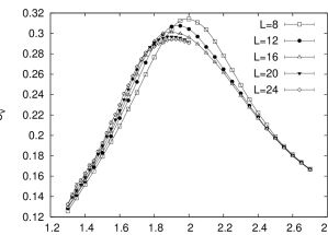
Figure 3: The specific heat as function of $T$ for various lattice sizes. The main feature is in the decrease and flattening of the peaks as $L$ increases.

The specific heat shows no tendency to diverge at all near the transition region. On the contrary, the peak of $C_{v}$ tends to slightly decrease and broaden as system size increases (see Fig. 3). This is probably an artifact due to the large slope of the path in the $(T,H)$ plane that we simulated [see Eq.(32)]. In fact, the larger the system size, the lower the peak height. However, note that the specific heat has a contribution (from the magnetic energy) with an explicit linear dependence on the field strength (also the magnetization depends strongly on it). Anyhow, this supports a scenario of negative (maybe vanishing) $\alpha$, as reported, for example, by Rieger and Young rieger_II , Riegerrieger_I , Middleton and Fishermiddleton in their simulation of the random field Ising model and in experiments. belanger We shall discuss further the specific heat in the following. At the time being, note that the peak position of $C_{v}$ may be fitted to the usual power law and we find

$$T_{c}=1.68(4)\,,$$ (36)

which is compatible with the estimate given in Eq. (35). This fit provides no information on the $\nu$ exponent ($\nu=2(2)$).

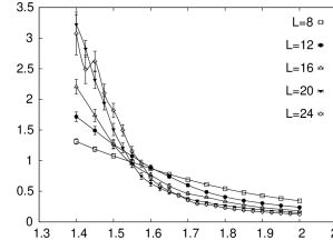
Figure 4: The cumulant $\xi/L$ as function of the temperature for various system sizes. Lines are interpolating splines and serve only as a guide to the eye. Note the noise in the curve for $L=24$ in all the crossing region.

We can extract further information on several exponents by means of the QM. Figure 4 shows a clear crossing of the ratio $\xi/L$ as function of $T$ for different values of $L$. Data for $L=20$ and $L=24$ are quite noisy, again due to difficulties in measuring the disconnected part of $G(k)$ [Eq. (II.2)] but still allow for locating a crossing temperature with other curves. As expected on general grounds, the crossing temperatures stay well away from the positions of the peak of $C_{v}$ and $\chi_{\mathrm{c}}$ but lie fairly close to the $T_{\mathrm{c}}^{\infty}$ value that has been extrapolated from the peaks position. Indeed, in the absence of scaling corrections, there should be no system size dependency of the crossing temperature. Such dependency, if any, carries important information on scaling corrections. quotient Unfortunately, in our case, there is no clear systematic dependence of $T_{\mathrm{cross}}$ on the lattice size as, for example, for small systems $T_{\mathrm{cross}}$ tends to shift to lower values as $L_{1}$ and $L_{2}$ increase, while it is sensibly shifted toward higher values when lattice size $L=20$ or $L=24$ is considered. This probably indicates that a crossover to first-order behavior is showing up.

We show in Table 2 our results for values of exponents $\alpha$, $\beta$, $\eta$ and $\overline{\eta}$, obtained from the QM. Unfortunately, we have not been able to measure $\partial_{\beta}\xi$ with enough precision to give a direct estimate for the thermal exponent $\nu$.

$L_{1},L_{2}$	$T_{\mathrm{cross}}$	$\eta$	$\overline{\eta}$	$\alpha/\nu$	$\beta/\nu$
8,12	1.6(2)	0.5(1)	-1.0(1)	0.091(6)	0.07(6)
8,16	1.54(6)	0.8(2)	-0.99(3)	0.07(2)	0.05(2)
8,20	1.55(2)	0.4(2)	-0.97(1)	0.070(1)	0.049(5)
8,24	1.58(2)	0.2(2)	-0.94(1)	0.083(1)	0.06(1)
12,16	1.5(1)	1.1(6)	-1.00(3)	0.07(2)	0.04(3)
12,20	1.53(4)	0.1(4)	-0.95(3)	0.08(1)	0.05(1)
12,24	1.57(4)	0.0(3)	-0.92(2)	0.087(7)	0.06(1)
16,20	1.55(5)	-0.5(8)	-0.90(4)	0.09(2)	0.056(4)
16,24	1.59(4)	-0.4(5)	-0.85(2)	0.09(1)	0.08(2)

Table 2: Exponents and crossing temperatures extracted with the QM applied to the intersection of the cumulant $\xi/L$.

Maybe the most striking result in Table 2 is the smallness of the $\beta$ exponent, indicating that the order parameter could be discontinuous at the transition. A similar behavior has been found for the RFIM rieger_I ; hartmann1 and in experiments. belanger A very small (but definitely positive) value of $\beta$ has been found also by Falicov et al. falicov by means of renormalization-group calculations for the binary RFIM. They also calculated magnetization curves as functions of the temperature and field strength, showing abrupt jumps at the transition point.

The value of $\overline{\eta}$ agrees with the one found in Ref. [ogielski, ],$\overline{\eta}=-1.0(3)$ and agrees with the smallness of the order parameter exponent and the estimate [Eq. (34)] of $\nu$ as the relation $\beta=(1+\overline{\eta})\nu/2$ holds. Note also that, given the value of $\eta$ from Eq. (33), the Schwartz-Sofferschwartz relations $2(\eta-1)\geq\overline{\eta}\geq-1$ are satisfied as equalities within errors. We see that, at larger sizes, the value of $\eta$ decreases down even to negative values (showing a large error) but is always compatible with our previous estimate (at least at two standard deviations): $\eta=0.4(1)$. Also the disconnected susceptibility diverges as $L^{3}$ (since $\overline{\eta}$ is very close to $-1$, because $\chi_{\mathrm{dis}}\propto L^{2-\overline{\eta}}$). As for the specific heat exponent, we know from the Harris criterion Harris that $\alpha$ should be negative or zero in a disordered second-order transition framework. Here we report values which are small but definitely positive. It is also true that if the specific heat had a cusplike singularity, our data would not allow to evaluate the asymptotic value for $C_{v}$, and the estimates for $\alpha$ would be meaningless.

Figure 5: The energy Binder cumulant as function of $T$ for all lattice sizes.

Figure 6: Scaling of the minima of Binder cumulant Eq. (37) (top) and of the minima positions (bottom). Fitting functions are also showed. In the bottom we have fixed $d_{g}/2$ to 3/2 in the fit. See section IV.2 for more details.

IV.2 First-order phase transition scenario

The analysis presented above, based on the hypothesis that a second-order transition is taking place, looks inconclusive. This is especially clear from exponent $\eta$, which lies so near to our prediction for a first-order phase transition: $\eta=0.5$. In addition this exponent in the Schwartz-Soffer inequality fixes the value of $\overline{\eta}$ to -1, and all our estimates of the $\overline{\eta}$ exponent are compatible with this value. Of course, this could be due to finite $L$ corrections to scaling, but we think that the phase transition is truly first-order.

We now proceed to show that our data are compatible with a weak first-order transition with a very large, but not diverging, correlation length at the transition point. A good observable to test is the Binder cumulant for the total energy density:binlau_II

$$g_{4}^{E}=\frac{1}{2}\left(3-\frac{\overline{\langle E^{4}\rangle}}{\overline{{\langle E^{2}\rangle}}^{2}}\right)\,,$$ (37)

which is usually easy to measure in simulations because of the good noise-to-signal ratio of the energy density. Notice that this Binder cumulant works directly on the averaged probability distribution of the energy. In both the disordered and ordered phases, well away from the transition temperature, the probability distribution of the energy $\overline{\langle P(E)\rangle}$ tends to a single delta function in the thermodynamic limit, so that $g_{4}^{E}\rightarrow 1$. In the case of a second-order transition this is also true at $T_{c}$, while in the presence of a first-order transition, we have an energy distribution with more than one sharp peak, so the infinite volume limit of $g_{4}^{E}$ is nontrivial. Challa et al.binlau_II obtained the expression for the nontrivial limit and finite size correction to leading order in the framework of a double Gaussian approximation for the multipeaked $\overline{\langle P(E)\rangle}$:

$$1-g_{4}^{E}(T^{*}) = g_{1}(E_{+},E_{-})$$

$$+ g_{2}(E_{+},E_{-},C_{v+},C_{v-})L^{-d}\,,$$

$$g_{1}(E_{+},E_{-}) = \frac{E_{+}^{4}+E_{-}^{4}}{\left(E_{+}^{2}+E_{-}^{2}\right)^{2}}-\frac{1}{2}\,,$$ (39)

where $T^{*}$ is the temperature at which the minimum (maximum of $1-g_{4}^{E}$) appears and $g_{2}$ is a complicated combination of the specific heats and energies of the infinite volume coexistent states ($+,-$). The term $g_{1}$ is vanishing if the latent heat $Q=E_{+}-E_{-}$ is zero.

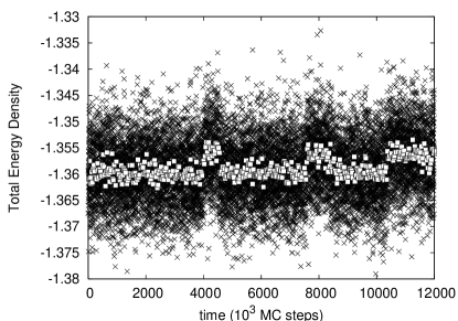
Figure 7: Monte Carlo histories of magnetic energy density (top), total energy density (middle) and staggered magnetization (bottom) for a typical sample of lattice size $L=24$ showing jumps between states at the transition temperature. The latent heat is clearer when binning 25 consecutive Monte Carlo measurements for the total energy (open symbols).

Our data for $1-g_{4}^{E}$ effectively show broad peaks at temperatures $T^{*}(L)$ shifting toward lower temperature values as $L$ increases (Fig. 5). We also expect from Eq. (27) that the critical temperature shift should scale as $T^{*}(L)-T_{c}\propto L^{-d/2}$.

The matching of the data with this model is impressive, (see Fig. 6). A power-law fit against $1-g_{4}^{E}(T^{*}(L))=g_{1}+g_{2}L^{-d_{g}}$ gives

$$g_{1} = 0(2)\times 10^{-4}\,,$$ (40)

$$d_{g} = 3.0(1)\,,$$ (41)

where we excluded in the fit the $L=8$ data [fitting also $L=8$ data brings $d_{g}=2.8(1)$ but $g_{1}$, even if compatible with zero, has an unphysical negative value]. The extrapolated transition temperature is (assuming a power $d_{g}/2=1.5$ and $L>8$)

$$T_{c}=1.64(2)\,.$$ (42)

with a reasonable $\chi^{2}/\mathrm{DOF}=0.6$. We also recall that susceptibility data gave $1/\nu=1.0(3)$ which is acceptable: an exponent $3/2$ is within two standard deviations.

However, the infinite volume limit of $1-g_{4}^{E}\left[T^{*}(L=\infty)\right]$ is very small, suggesting a zero latent heat for the transition. Actually, we will show below that one can estimate from $g_{1}$ the order of magnitude of the latent heat, which will turn out to be in agreement with metastability estimates.

IV.3 Metastability

A very small latent heat may be very hard to detect due to large thermal and sample-to-sample (disorder) fluctuations. If this is the case, it should be possible to detect the latent heat by exploring the behavior of single samples.

Indeed, for our largest systems ($L=24$), around 20% of the samples started to display metastability between a disordered, small $M_{\mathrm{s}}$ state and a large $M_{\mathrm{s}}$ state. This behavior was not detected on smaller systems. Furthermore, for a large fraction of the samples, the metastability on $M_{\mathrm{s}}$ was correlated with a metastability in the internal energy and in the magnetization density. This can be observed, for instance, in the Monte Carlo history at temperature $T=1.5$ ($H=2.25$) shown in Fig. 7 for a $L=24$ sample. Note that the fluctuations for the internal energy were huge. However, if one bins 25 consecutive Monte Carlo measurements (white squares in the central plot) metastability is very clear.

We also learn from Fig. 7 that the probability distribution for the staggered magnetization shows three clear peaks, one for a disordered state and two for a quasisymmetric ordered phase. The transition time is of the order of $~{}10^{6}$ MC steps (and tunneling is probably sped up by our use of parallel tempering). It is then clear that some of the samples may not have had enough time during the simulation ($2.4\times 10^{7}$ MC steps) to perform enough transitions between metastable states to give a correct value for the mean staggered magnetization, and this explains the noise we found in observables involving connected functions (susceptibilities, correlation length and specific heat).

One can estimate the latent heat and the mean energy from Fig. 7 (recall $L=24$): $Q\simeq 0.005$ and $E_{+}\simeq E_{-}=E\simeq 1.36$. We can introduce these values in the equation from $g_{1}$ [see Eq. (II.4)]. For small latent heat (we write only the dominant term) it is possible to obtain

$$1-g=g_{1}\simeq\frac{Q}{4E^{3}}$$ (43)

obtaining $g_{1}=5\times 10^{-4}$, only at two standard deviations of the $g_{1}$ value computed by extrapolating the Binder cumulant.

V CONCLUSIONS

We have studied the three dimensional diluted antiferromagnetic Ising model in a magnetic field using equilibrium numerical techniques and analysis methods.

We have found that the data can be described in the framework of a second phase transition, and obtained critical exponents are compatible with those obtained by Ogielski and Huse. ogielski However, the critical exponent for the order parameter is very small, which points to a first-order transition. Note, however, that similarly small values of this critical exponent were found in ground-state investigations both for the DAFF hartmann1 (at different dilutions) and for the Gaussian RFIM hartmann1 ; middleton (these authors claimed that the phase transition was continous). Nevertheless, by studying the Binder cumulant of the energy, we obtained clear indications on our largest lattices of a weak first-order phase transition. Furthermore, on our largest systems, a large number of samples show flip-flops between the ordered (quasidegenerated) and disordered phases both in the energy as well as in the order parameter, which again is a strong evidence for the weakly first-order scenario.

We remark that a complete theory of scaling in disordered first-order phase transitions (in line with that of Ref. [binlau_II, ] for ordered systems) is still lacking. However, we have proposed a set of effective exponents and have shown that this scaling accounts for our data.

Appendix A Scaling in first-order phase transitions in presence of disorder

It is straightforward to use the Cauchy-Schwartz inequality to obtain a bound on the $p$ derivative of an arbitrary observable. This bound will hold both for first- and second-order phase transitions. Following the lines of reasoning of Ref. [chayes, ] we get

$$\frac{d\overline{\langle A\rangle}}{dp}\leq a\sqrt{\overline{\langle A^{2}\rangle}}L^{d/2}\,.$$ (44)

We recall that $p$ is the dilution of the model, and $a^{2}=1/[p(1-p)]$. Notice that this inequality holds for any temperature, dilution and lattice size.

Assuming now that $\sqrt{\overline{\langle A^{2}\rangle}}$ is of the same order of magnitude of $\overline{\langle A\rangle}$ (which is certainly the case for the internal energy), we translate Eq. (44) into a bound for the logarithmic derivative:

$$\frac{d\log\overline{\langle A\rangle}}{dp}\leq L^{d/2}\,,$$ (45)

Now, the logarithmic derivative tells us about the width of the critical region on a finite system. For instance, at a given temperature and magnetic field, let $p(L)$ be the spin dilution at a susceptibility peak and $p_{c}$ the thermodynamic limit of any such quantity. We then expect $p(L)-p_{c}\propto L^{-d/2}$. Notice that the notion of a critical region permits us to define an effective $\nu$ exponent as $p(L)-p_{c}\propto L^{-1/\nu}$. Hence,

$$\nu\geq\frac{2}{d}\,.$$ (46)

If the coexistence line has finite slope in the ($T$,$p$) plane, it is clear that the critical width in dilution is proportional to the critical width in temperature. A similar argument holds for the derivative with respect to the magnetic field. Thus, the logarithmic derivative with respect to temperature or magnetic field of $A$ may diverge (at most) as fast as $L^{d/2}$. So, we have found an upper bound for the divergences of the specific heat and connected susceptibilities (both are derivatives of the energy and magnetization respectively): they cannot diverge, with the lattice size, with an exponent greater than $d/2$.

Let us also remark that in footnote 7 of Ref. [chayes, ] it is reported that $\nu=2/d$ for first-order transitions in the presence of disorder but without an explanation of this fact.

Finally we will show that the Schwartz-Soffer schwartz inequality also holds in a first-order phase transition scenario. Schwartz and Soffer show that

$$\hat{\chi}_{\mathrm{c}}^{M_{s}}(q)\leq\frac{1}{h}\sqrt{\hat{\chi}_{\mathrm{dis}}^{M_{s}}(q)}\,,$$ (47)

where $q$ is the momentum, $h$ is the standard deviation of the magnetic field and $\hat{\chi}_{\mathrm{c}}^{M_{s}}(q)$ and $\hat{\chi}_{\mathrm{dis}}^{M_{s}}(q)$ are the Fourier transforms of the connected susceptibility and the disconnected part of it respectively. schwartz In order to obtain the inequality, we introduce the minimum momenta available which is of order $1/L$, and use $\chi(L)=\hat{\chi}_{\mathrm{c}}^{M_{s}}(q_{\mathrm{min}})$ and $\chi_{\mathrm{dis}}(L)=\hat{\chi}_{\mathrm{dis}}^{M_{s}}(q_{\mathrm{min}})$. On the other hand, in a first-order phase transition, we define the effective exponents $\eta$ and $\overline{\eta}$ by means of the scaling of the susceptibilities at the critical point: $\chi(L)\simeq L^{2-\eta}$ and $\chi_{\mathrm{dis}}(L)\simeq L^{2-\overline{\eta}}$. All together, we obtain the Schwartz-Soffer inequality:

$$\frac{2-\overline{\eta}}{2}\geq 2-\eta\,.$$ (48)

Note that we have not used the criticality properties of the propagators.

References

- (1) D. P. Belanger, Experiments on the Random Field Ising Model in Spin Glasses and Random Fields, edited by A. P. Young (World Scientific, Singapore, 1997).
- (2) T. Nattermann,Theory of the Random Field Ising Model in Spin Glasses and Random Fields, edited by A. P. Young (World Scientific, Singapore, 1997).
- (3) N. Sourlas, Comp. Phys. Comm. 121, 183 (1999).
- (4) G. Parisi and N. Sourlas, Phys. Rev. Lett. 89, 257204 (2002).
- (5) S. Fishman and A. Aharony, J. Phys. C 12 L729 (1979).
- (6) J. L. Cardy, Phys. Rev. B 29, 505 (1984).
- (7) A. T. Ogielski and D. A. Huse, Phys. Rev. Lett. 56, 1298 (1986).
- (8) A few samples in a lattice were simulated.
- (9) A. K. Hartmann and U. Nowak, Eur. Phys. J. B 7, 105, (1999).
- (10) A. Aharony, Phys. Rev. B 18, 3318, (1978)
- (11) H. Rieger and A. P. Young, J. Phys. A: Math. Gen. 26 5279 (1993).
- (12) H. Rieger, Phys. Rev. B 52, 6659 (1995).
- (13) L. Hernandez and H. T. Diep, Phys. Rev. B 55, 14080 (1997).
- (14) J. Machta, M. E. J. Newman and L. B. Chayes, Phys. Rev. E 62, 8782 (2000).
- (15) A. J. Bray and M. A. Moore, J. Phys. C 18, L927, (1985).
- (16) A. K. Hartmann and A. P. Young, Phys. Rev. B 64, 214419 (2001).
- (17) A. A. Middleton, D. S. Fisher, Phys. Rev. B 65, 134411 (2002).
- (18) M. Tesi, E. Janse van Resburg, E. Orlandini and S. G. Whillington, J. Stat. Phys. 82, 155 (1996); K. Hukushima and K. Nemoto, J. Phys Soc. Jpn. 65, 1604 (1996); E. Marinari, G. Parisi and J. J. Ruiz-Lorenzo,Numerical Simulations of Spin Glass Systems in Spin Glasses and Random Fields, edited by A. P. Young (World Scientific, Singapore, 1997).
- (19) H. G. Ballesteros, L. A. Fernández, V. Martín-Mayor and A. Muñoz Sudupe. Phys. Lett. B378, 207 (1996).
- (20) F. Cooper, B. Freedman and D. Preston, Nucl. Phys. B 210, 210 (1989).
- (21) J. T. Chayes, L. Chayes, D.S. Fisher and T. Spencer, Phys. Rev. Lett. 57, 2999 (1986).
- (22) D. Stauffer and A. Aharony in Introduction to the percolation theory. (Taylor and Francis, London 1984).
- (23) M. N. Barber, Finite Size Scaling in Phase Transitions and Critical Phenomena, edited by C. Domb and J. L. Lebowitz (Academic Press 1983) volume 8.
- (24) K. Binder and D. P. Landau, Phys. Rev. B 30, 1477 (1984).
- (25) M. S. S. Challa, D. P. Landau and K. Binder, Phys. Rev. B 34, 1841 (1986).
- (26) K. Binder, Rep. Prog. Phys. 50, 783 (1987).
- (27) C. Chatelain, B. Berche, W. Janke and P. E. Berche, Phys Rev. E 64, 036120 (2001).
- (28) We recall that they obtained their estimates of the critical temperature and exponents by simulating in the paramagnetic phase, without perform finite size scaling, and by fitting the largest lattice simulated to the standard law, for example for the susceptibility: .
- (29) A. Falicov, A. N. Berker and S. R. McKay, Phys. Rev. B 51, 8266 (1995).
- (30) M. Schwartz and A. Soffer, Phys. Rev. Lett. 55, 2499 (1985).
- (31) A. B. Harris, J. Phys. C 7, 1671 (1974).