Searching for Gravitational Radiation from Binary Black Hole MACHOs in the Galactic Halo

A Thesis Submitted in
Partial Fulfillment of the
Requirements for the degree of

Doctor of Philosophy

in
Physics

at

The University of Wisconsin–Milwaukee

December 2004

A Thesis Submitted in
Partial Fulfillment of the
Requirements for the degree of

Doctor of Philosophy

in
Physics

at

The University of Wisconsin–Milwaukee

December 2004

          Patrick Brady Date

    Graduate School Approval Date

© Copyright 2004
by
Duncan A. Brown

to
Mum and Dad

Preface

The work presented in this thesis stems from my participation in the LIGO Scientific Collaboration.

The upper limit on the rate of binary neutron star inspirals quoted in chapter 1 is based on

B. Abbott et al. (The LIGO Scientific Collaboration), “Analysis of LIGO data for gravitational waves from binary neutron stars,” Phys. Rev. D 69 (2004) 122001.

Chapter 5 is based on material from

Duncan A. Brown et al., “Searching for Gravitational Waves from Binary Inspirals with LIGO,” Class. Quant. Grav. 21, S1625 (2004).

and

B. Abbott et al. (The LIGO Scientific Collaboration), “Search for binary neutron star coalescence in the Local Group,” to be submitted to Class. Quant. Grav.

Chapter 6 is based on

Duncan A. Brown (for the LIGO Scientific Collaboration), “Testing the LIGO inspiral analysis with hardware injections,” Class. Quant. Grav. 21, S797 (2004).

Chapter 7 is based on

B. Abbott et al. (The LIGO Scientific Collaboration), “Search for binary black hole MACHO coalescence in the Galactic Halo,” to be submitted to Phys. Rev. D

Conventions

There are two possible sign conventions for the Fourier transform of a time domain quantity $v(t)$. In this thesis, we define the Fourier transform $\tilde{v}(f)$ of a $v(t)$ to be

$$\tilde{v}(f)=\int_{-\infty}^{\infty}dt\,v(t)\,e^{-2\pi ift}$$

and the inverse Fourier transform to be

$$v(t)=\int_{-\infty}^{\infty}df\,\tilde{v}(f)\,e^{2\pi ift}.$$

This convention differs from that used in some gravitational wave literature, but is the adopted convention in the LIGO Scientific Collaboration.

The time-stamps of interferometer data are measured in Global Positioning System (GPS) seconds: seconds since 00:00.00 UTC January 6, 1980 as measured by an atomic clock.

Astronomical distances are quoted in parsecs

$$1\,\mathrm{pc}=3.0856775807\times 10^{16}\,\mathrm{m}$$

and masses in units of solar mass

$$1\,\mathrm{M}_{\odot}=1.98892\times 10^{30}\,\mathrm{kg}.$$

List of Tables

1. 1 Mean and Variance of the Matched Filter Output for Gaussian Noise
2. 1 Data Quality Cuts Available During S2
3. 2 Inspiral Triggers Generated at Times of Data Quality Cuts
4. 3 Choice of Data Quality Cuts in S2
5. 4 Fake Science Segments Used to Test DAG Generation
6. 1 Hardware Injections Found by the Analysis Pipeline
7. 1 Pipeline Parameters used in S2 BBHMACHO Search

List of Figures

1. 1 Effect of a Gravitational Wave on Test Particles
2. 2 Effect of a Gravitational Wave Polarizations on a Ring of Particles
3. 3 Location of LIGO Interferometers
4. 4 Optical Configuration of LIGO
5. 5 Fundamental Noise Sources of Initial LIGO
6. 6 Differential mode control servo loop
7. 7 Coordinates Used to Describe Gravitational Radiation from a Binary
8. 8 Coordinates Used to Describe the Response of a Gravitational Wave Interferometer
9. 9 Antenna Response of an Interferometer
10. 1 H1 Rotation Curve of NGC 3198
11. 2 Scattering of Light in Schwarzschild Spacetime
12. 3 Gravitational Lensing of Light By a MACHO
13. 4 Sensitivity of LIGO to a Binary Black Hole MACHO Inspiral
14. 5 Histogram of BBHMACHO Monte Carlo Mass Distribution
15. 6 Spatial Distribution of Binary Black Hole MACHOs in Galactocentric Coordinates
16. 7 Spatial Distribution of Binary Black Hole MACHOs Seen From Earth
17. 1 Distribution of the Filter Output for Gaussian Noise
18. 2 Impulse Response of Matched Filter With a Constant Power Spectrum
19. 3 Impulse Response of Matched Filter With a Real Power Spectrum
20. 4 Wrap-around of the Matched Filter
21. 5 Distribution of Filter Output Using Median Power Spectral Estimator
22. 6 Impulse Response of Matched Filter With a Truncated Power Spectrum
23. 7 Output of the Filtering Code for a Chirp In the Absence of Noise
24. 8 Inspiral Trigger Selection Algorithm
25. 1 Simple Pipeline to Search Data From Two Interferometers
26. 2 Largest Inspiral Trigger Seen in the S1 Analysis
27. 3 Loss in Signal-to-noise Ratio Due to Resampling
28. 4 Algorithm Used to Divide Science Segments into Data Analysis Segments
29. 5 Binary Black Hole MACHO Template Bank
30. 6 Ratio of Effective Distance of Injected Signals Between Observatories
31. 7 Trigger Coincidence Test
32. 8 Auxiliary Channel Veto Investigation of Two Candidate Triggers
33. 9 Sensitivity of LIGO Interferometers During S2
34. 10 Structure of the S2 Triggered Search Pipeline
35. 1 Schematic of LIGO Interferometer Showing Injection Points
36. 2 Candidate Events from Hardware Injections
37. 3 Study of Calibration Using Hardware Injections
38. 4 Study of Veto Safety Using Hardware Injections
39. 1 Amounts of Single and Coincident Interferometer Data in S2
40. 2 MACHO Template Bank Size for Various Lower Masses
41. 3 S2 Interferometer Ranges and Template Bank Size
42. 4 Tuning the $\chi^{2}$ Veto for H1
43. 5 Found and Missed H1 Injections for $\Xi=12.5\delta^{2}=0.04$
44. 6 Illustration of Tuning Based on Injections
45. 7 Signal-to-noise ratio and $\chi^{2}$-veto for Injected Signals
46. 8 Injections Detected and Missed by Monte Carlo Simulation
47. 9 Search Efficiency as a Function of Chirp Mass
48. 10 Measurement accuracy of L1 Injection Parameters
49. 11 Measurement accuracy of H1 Injection Parameters
50. 12 Measurement accuracy of H2 Injections Parameters
51. 13 Background Triggers from 20 Time Slides
52. 14 Comparison of Background Triggers and Injections
53. 1 Comparison of Best LIGO Interferometer Sensitivity

Chapter 1 Introduction

One of the earliest predictions of the Theory of General Relativity was the existence of gravitational waves. By writing the metric $g_{\mu\nu}$ as the sum of the flat Minkowski metric $\eta_{\mu\nu}$ and a small perturbation $h_{\mu\nu}$,

$$g_{\mu\nu}=\eta_{\mu\nu}+h_{\mu\nu},$$ (1.1)

and considering bodies with negligible self-gravity, Einstein showed[Einstein:1916]

“that these $h_{\mu\nu}$ can be calculated in a manner analogous to that of the retarded potentials of electrodynamics.”

It follows that gravitational fields propagate at the speed of light. In electrodynamics, the lowest multipole moment that produces radiation is the electric dipole; there is no electric monopole radiation due to the conservation of electric charge. Similarly in General Relativity, the lowest multipole that produces gravitational waves is the quadrupole moment. Radiation from the mass monopole, mass dipole and momentum dipole vanish due to conservation of mass, momentum and angular momentum respectively. Einstein also derived the quadrupole formula for the gravitational wave field, which states that the spacetime perturbation is proportional to the second time derivative of the quadrupole moment of the source. The strength of the gravitational waves decreases as the inverse of the distance to the source. We can estimate this strength at a distance $r$ by noticing that the quadrupole moment involves terms of dimension mass $\times$ length² and so the second time derivative of the quadrupole moment is proportional to the kinetic energy of the source associated with non-spherical motion $E^{\mathrm{ns}}_{\mathrm{kin}}$. Using the quadrupole formula, which we will see in equation (2.63), we then approximate the strength of the gravitational waves as

$$h\sim\frac{G}{c^{4}}\frac{E^{\mathrm{ns}}_{\mathrm{kin}}}{r}.$$ (1.2)

The effect of a gravitational wave is to cause the measured distance $L$ between two freely falling bodies to change by a distance $\Delta L\sim hL$.

Interferometers were suggested as a way of measuring the change in length between two test masses by Pirani in 1956[Pirani:1956] and the first working detector was constructed by Forward in 1971[Forward:1971]. The fundamental designs of modern laser interferometers were developed by Weiss[Weiss:1972] and Drever[Drever:1980] in the 1970s. The principle upon which interferometric detectors operate is to use laser light to measure the change in distance between two mirrors as a gravitational wave passes through the detector. The sensitivity of an interferometer on the Earth is limited by gravity gradient noise at frequencies below $\sim 5$ Hz[Saulson:1994]. Any time changing distribution of matter near the detector, for example compression waves in the Earth, cause fluctuations in the local gravitational field. These fluctuations will cause the test masses to move producing a spurious response in the interferometer which masks the presence of gravitational waves. In fact, Earth based interferometers are typically limited in sensitivity to frequencies above $\sim 10$ Hz due to the seismic motion of the earth.

The canonical example of an astrophysical source of gravitational waves is the Hulse-Taylor binary pulsar, PSR $1913+16$[1975ApJ...195L..51H]. This system is composed of two neutron stars, each of mass $\sim 1.4\,M_{\odot}$, with average separation and orbital velocity of $\sim 10^{9}$ m and $\sim 10^{5}$ms^-1, respectively. The period of the orbit is $7.75$ hours and the binary is at a distance from the earth of $\sim 6$ kpc. Hulse and Taylor observed that the orbital period of the binary is decreasing and that the rate of orbital energy loss agrees with the expected loss of energy due to the radiation of gravitational waves to within $0.3\%$[Taylor:1982, Taylor:1989]. Since the quadrupole moment of an equal mass binary is periodic at half the orbital period, we would expect the frequency of the gravitational waves emitted to be twice the orbital frequency. Thus, the gravitational waves from PSR $1913+16$ have a frequency $f_{\mathrm{GW}}\sim 10^{-4}$ Hz that is outside the sensitive band of earth based detectors. Nevertheless, the orbit will continue to tighten by gravitational wave emission, and the two neutron stars are expected to merge in about 300 million years; in the last several minutes prior to merger, the gravitational wave frequency will sweep upward from $\sim 10$ Hz reaching about 1500 Hz just before the merger.

It is worthwhile to estimate the strength of the gravitational waves from a neutron star binary since it informs the target sensitivity for modern interferometric detectors. The non-spherical kinetic energy of this system is

$$E_{\mathrm{kin}}^{\mathrm{ns}}\sim 1.4\,\mathrm{M}_{\odot}(\pi a/T)^{2}$$ (1.3)

where $T$ is the binary period and $a$ is the average separation. The period, separation and mass of a binary are related by Kepler’s third law,

$$T^{2}=\frac{4\pi^{2}}{GM}a^{3},$$ (1.4)

where $M$ is the total mass of the binary. Using equation (1.2), Kepler’s third law and the non-spherical kinetic energy given in equation (1.3), we can estimate the strength of the waves from a neutron star binary as

$$h\sim 10^{-20}\times\left(\frac{6.3\,\mathrm{kpc}}{r}\right)\left(\frac{M}{2.8M_{\odot}}\right)^{5/3}\left(\frac{T}{1\,\mathrm{s}}\right)^{-\frac{2}{3}}.$$ (1.5)

When the orbital separation is $a\sim 10^{5}$ m, the orbital period will be $T\sim 10^{-2}$ seconds and the gravitational wave strain will be $h\sim 10^{-19}$.

To date, four binary neutron star systems that will merge within a Hubble time have been discovered. By considering the time to merger, position and efficiency of detecting such binary pulsar systems, the galactic merger rate for inspirals can be estimated[Phinney:1991ei]. The latest estimates of neutron star inspirals in the Milky Way are $8.3\times 10^{-6}$ yr^-1. Extrapolating this rate to the neighboring Universe using the blue-light luminosity gives an (optimistic) estimate of the rate at $0.3$ yr^-1 within a distance of $\sim 20$ Mpc. To measure the waves from a neutron star binary at this distance, we must construct interferometers that are sensitive to gravitational waves of strength $h\sim 10^{-22}$. An overview of the theory and experimental techniques underlying the generation and detection of gravitational waves from binary inspiral is presented in chapter 2.

A world-wide network of gravitational wave interferometers has been constructed that have the sensitivity necessary to detect the gravitational waves from astrophysical sources. Among these is the Laser Interferometric Gravitational Wave Observatory (LIGO)[Barish:1999]. LIGO has completed three science data taking runs. The first, referred to as S1, lasted for 17 days between August 23 and September 9, 2002; the second, S2, lasted for 59 days between February 14 and April 14, 2003; the third, S3, lasted for 70 days between October 31, 2003 and January 9, 2004. During the runs, all three LIGO detectors were operated: two detectors at the LIGO Hanford observatory (LHO) and one at the LIGO Livingston observatory (LLO). The detectors are not yet at their design sensitivity, but the detector sensitivity and amount of usable data has improved between each data taking run. The noise level is low enough that searches for coalescing compact neutron stars are worthwhile, and since the start of S2, these searches are sensitive to extra-galactic sources. Using the techniques of matched filtering described in chapter 4 of this dissertation, the S1 binary neutron star search set an upper limit of

$$\mathcal{R}_{90\%}<1.7\times 10^{2}\;\textrm{per year per Milky Way Equivalent Galaxy (MWEG)}$$ (1.6)

with no gravitational wave signals detected. Details of this analysis can be found in [LIGOS1iul].

In this dissertation, we are concerned with the search for gravitational waves from a different class of compact binary inspiral: those from binary black holes in the galactic halo. Observations of the gravitational microlensing of stars in the Large Magellanic cloud suggest that $\sim 20\%$ of the galactic halo consists of objects of mass $\sim 0.5\,M_{\odot}$ of unknown origin. In chapter 3 we discuss a proposal that these Massive Astrophysical Compact Halo Objects (MACHOs) may be black holes formed in the early universe and that some fraction of them may be in binaries whose inspiral is detectable by LIGO[Nakamura:1997sm]. The upper bound on the rate of such binary black hole MACHO inspirals are projected to be $R\sim 0.1$ yr^-1 for initial LIGO, much higher than the binary neutron star rates discussed above. It should be noted however, that while binary neutron stars have been observed, there is no direct observational evidence of the existence of binary black hole MACHOs. Despite this, the large projected rates make them a tempting source for LIGO. In chapter 5 we describe an analysis pipeline that has been used to search the LIGO S2 data for binary black hole MACHOs. Chapter 6 describes how the search techniques were tested on data from the gravitational wave interferometers. Finally we present the result of the S2 binary black hole MACHO search in chapter 7.

Chapter 2 Gravitational Radiation from Binary Inspiral

In this chapter we review some of the physics underlying the detection of gravitational waves from binary inspiral. In section 2.1 we review the effect of gravitational waves on a pair of freely falling particles in order to introduce some of the concepts that we need to discuss the detection of gravitational waves from binary inspiral. For a detailed description of gravitational waves, we refer to [MTW73, Thorne:1982cv]. Section 2.2 describes how a laser interferometer can be used to measure this effect. The gravitational waveform produced by the inspiral of two compact objects, such as neutron stars or black holes, are discussed in section 2.3. We also derive the waveform that will be used to search for gravitational waves from binary inspiral events in the Universe.

2.1 The Effect of Gravitational Waves on Freely Falling Particles

The 4-velocity $\vec{u}$ of a freely falling test particle satisfies the geodesic equation[Wald:1984]

$$\left(\nabla_{\vec{u}}\vec{u}\right)^{\alpha}=u_{\phantom{\alpha};\mu}^{\alpha\phantom{;\mu}}u^{\mu}=0,$$ (2.1)

where ; denotes the covariant derivative, that is,

$$u_{\phantom{\alpha};\mu}^{\alpha\phantom{;\mu}}u_{\phantom{\mu}}^{\mu}=\left(u_{\phantom{\alpha},\mu}^{\alpha\phantom{,\mu}}+\Gamma^{\alpha}_{\mu\nu}u^{\nu}\right)u^{\mu},$$ (2.2)

where $\Gamma^{\alpha}_{\mu\nu}$ is the connection coefficient of the metric $g_{\mu\nu}$ and $,\mu$ represents the standard partial derivative with respect to the coordinate $x^{\mu}$.

Consider two particles $A$ and $B$, as shown in figure 1 (a), with separation vector $\vec{\xi}$. The particles are initially at rest with respect to each other, so

$$\nabla_{\vec{u}}\vec{u} =0,$$ (2.3)

$$\vec{u}\cdot\vec{\xi} =0.$$ (2.4)

If the spacetime is curved, the second derivative of $\vec{\xi}$ along $\vec{u}$ is non-zero; it is given by the equation of geodesic deviation

$$\nabla_{\vec{u}}\nabla_{\vec{u}}\vec{\xi}=-R(\_,\vec{u},\vec{\xi},\vec{u}),$$ (2.5)

where $R(\_,\vec{u},\vec{\xi},\vec{u})$ is the Riemann curvature tensor. If the spacetime is flat with weak gravitational waves propagating in it, we can describe it by a metric

$$g_{\mu\nu}=\eta_{\mu\nu}+h_{\mu\nu},$$ (2.6)

where $h_{\mu\nu}$ is the perturbation to the metric due to the gravitational waves and $\eta_{\mu\nu}$ is the flat Minkowski metric . We now introduce a Local Lorentz Frame (LLF) for particle $A$. The LLF of particle $A$ is a coordinate system $x^{\alpha}$ in which

$$g_{\mu\nu}(A)=\eta_{\mu\nu}$$ (2.7)

and

$$g_{\mu\nu,\alpha}(A)=0,$$ (2.8)

where $g_{\mu\nu}(A)$ is the value of the metric at point $A$. This LLF is equivalent to a Cartesian coordinate system defined by three orthogonally pointing gyroscopes carried by particle $A$. The curvature of spacetime means that the coordinate system is not exactly Cartesian, but it can be shown that this deviation is second order in the spatial distance from the particle[MTW73]. This means that along the worldline of particle $A$ the metric is

$$g_{\mu\nu}=\eta_{\mu\nu}+\frac{\mathcal{O}\left(|\vec{x}|^{2}\right)}{R^{2}}$$ (2.9)

where $\vec{x}$ is the distance from the particle and $R\sim|R_{\alpha\beta\gamma\delta}|$. We can write the Cartesian coordinates of the LLF of $A$ as $x^{\mu}=(x^{0},x^{i})$, where $x^{0}=t$ is the timelike coordinate and $x^{i}$ are the three Cartesian coordinates. Then in the LLF of particle $A$ the equation of geodesic deviation becomes

$$\frac{\partial^{2}\xi^{j}}{\partial t^{2}}=-R_{\phantom{j}\alpha\beta\gamma}^{j\phantom{\alpha\beta\gamma}}u^{\alpha}\xi^{\beta}u^{\gamma}=-R_{\phantom{j}0k0}^{j\phantom{0k0}}\xi^{k},$$ (2.10)

since $u=(1,0,0,0)$. The presence of the gravitational waves are encoded in the curvature $R_{\alpha\beta\gamma\delta}$ which satisfies the wave equation

$$\eta^{\mu\nu}R_{\alpha\beta\gamma\delta,\mu\nu}=0.$$ (2.11)

In the Local Lorentz frame, the components of $\vec{\xi}$ are just the coordinates of $B$. In the LLF of $A$ we may write

$$\xi^{j}=\xi_{(0)}^{j}+\delta\xi^{j},$$ (2.12)

where $\xi_{(0)}^{j}$ is the unperturbed location of particle $B$ and $\delta\xi^{j}$ is the change in the position of $B$ caused by the gravitational wave. Substituting equation (2.12) into the equation of geodesic deviation, we obtain

$$\frac{\partial^{2}\delta\xi^{j}}{\partial t^{2}}\approx-R_{\phantom{j}0k0}^{j\phantom{0k0}}\xi_{(0)}^{k}=-R_{j0k0}\xi_{(0)}^{k},$$ (2.13)

where we have used $\eta_{\mu\nu}$ to lower the spatial index $j$ of the Riemann tensor. For a weak gravitational wave, all the components of $R_{\alpha\beta\gamma\delta}$ are completely determined by $R_{j0k0}$. Furthermore, it can be shown that the $3\times 3$ symmetric matrix $R_{j0k0}$, which we would expect to have $6$ independent components, has only $2$ independent components due to the Einstein equations and the Biancci identity. We define the (transverse traceless) gravitational wave field, $h_{jk}^{\mathrm{TT}}$, by

$$-\frac{1}{2}\frac{\partial^{2}h_{jk}^{\mathrm{TT}}}{\partial t^{2}}\equiv R_{j0k0}^{\mathrm{TT}}.$$ (2.14)

Using this definition in equation (2.13), we obtain

$$\delta\xi^{j}=\frac{1}{2}h_{jk}^{\mathrm{TT}}\xi_{(0)}^{k}.$$ (2.15)

If we orient our coordinates so the gravitational waves propagate in the $z$-direction, so $h_{jk}^{\mathrm{TT}}(t-z)$, then the only non-zero components of $h_{jk}^{\mathrm{TT}}$ are $h_{xx}^{\mathrm{TT}}$, $h_{yy}^{\mathrm{TT}}$, $h_{xy}^{\mathrm{TT}}$ and $h_{yx}^{\mathrm{TT}}$. Since $h_{jk}^{\mathrm{TT}}$ is symmetric and traceless, these components satisfy

$$h_{xx}^{\mathrm{TT}} =-h_{yy}^{\mathrm{TT}},$$ (2.16)

$$h_{xy}^{\mathrm{TT}} =h_{yx}^{\mathrm{TT}}.$$ (2.17)

For two more particles $C$ and $D$ separated by

$$\zeta^{j}=\zeta^{j}_{(0)}+\delta\zeta^{j},$$ (2.18)

as shown in figure 1 (b), the effect of the gravitational wave is then given by

$$\delta\zeta^{j}=\frac{1}{2}h_{jk}^{\mathrm{TT}}\zeta_{(0)}^{k}.$$ (2.19)

Taking the two particles $A$ and $B$ to lie on the $x$-axis of the LLF of particle $A$ with separation $x_{(0)}$, without loss of generality, we may write

$$\xi=(x_{(0)}+\delta x,0,0),$$ (2.20)

where $\delta x$ is the displacement of particle $B$ caused by the gravitational wave. Similarly, if particles $C$ and $D$ lie on the $y$-axis of the LLF of particle $C$ with separation $y_{(0)}$, we may write

$$\zeta=(0,y_{(0)}+\delta y,0)$$ (2.21)

where $\delta y$ is the displacement of particle $D$ caused by the gravitational wave.

We define the two independent components of the gravitational wave to be

$$h_{+} =h_{xx}^{\mathrm{TT}}=-h_{yy}^{\mathrm{TT}},$$ (2.22)

$$h_{\times} =h_{xy}^{\mathrm{TT}}=h_{yx}^{\mathrm{TT}}$$ (2.23)

which we call the plus and cross polarizations of the gravitational wave respectively. The influence of a linearly $+$ polarized gravitational wave propagating in the $z$-direction on the particles $A,B,C,D$ is then given by substituting equations (2.20) and (2.21) into (2.15) and (2.19) respectively to obtain

$$\delta x(t-z) =\frac{1}{2}h_{xx}^{\mathrm{TT}}(t-z)x_{(0)},$$ (2.24)

$$\delta y(t-z) =-\frac{1}{2}h_{yy}^{\mathrm{TT}}(t-z)y_{(0)}$$ (2.25)

Similarly, for a linearly $\times$ polarized gravitational wave propagating in the $z$-direction the effect on the particles is

$$\delta x(t-z) =\frac{1}{2}h_{xy}^{\mathrm{TT}}(t-z)y_{(0)},$$ (2.26)

$$\delta y(t-z) =\frac{1}{2}h_{yx}^{\mathrm{TT}}(t-z)x_{(0)}.$$ (2.27)

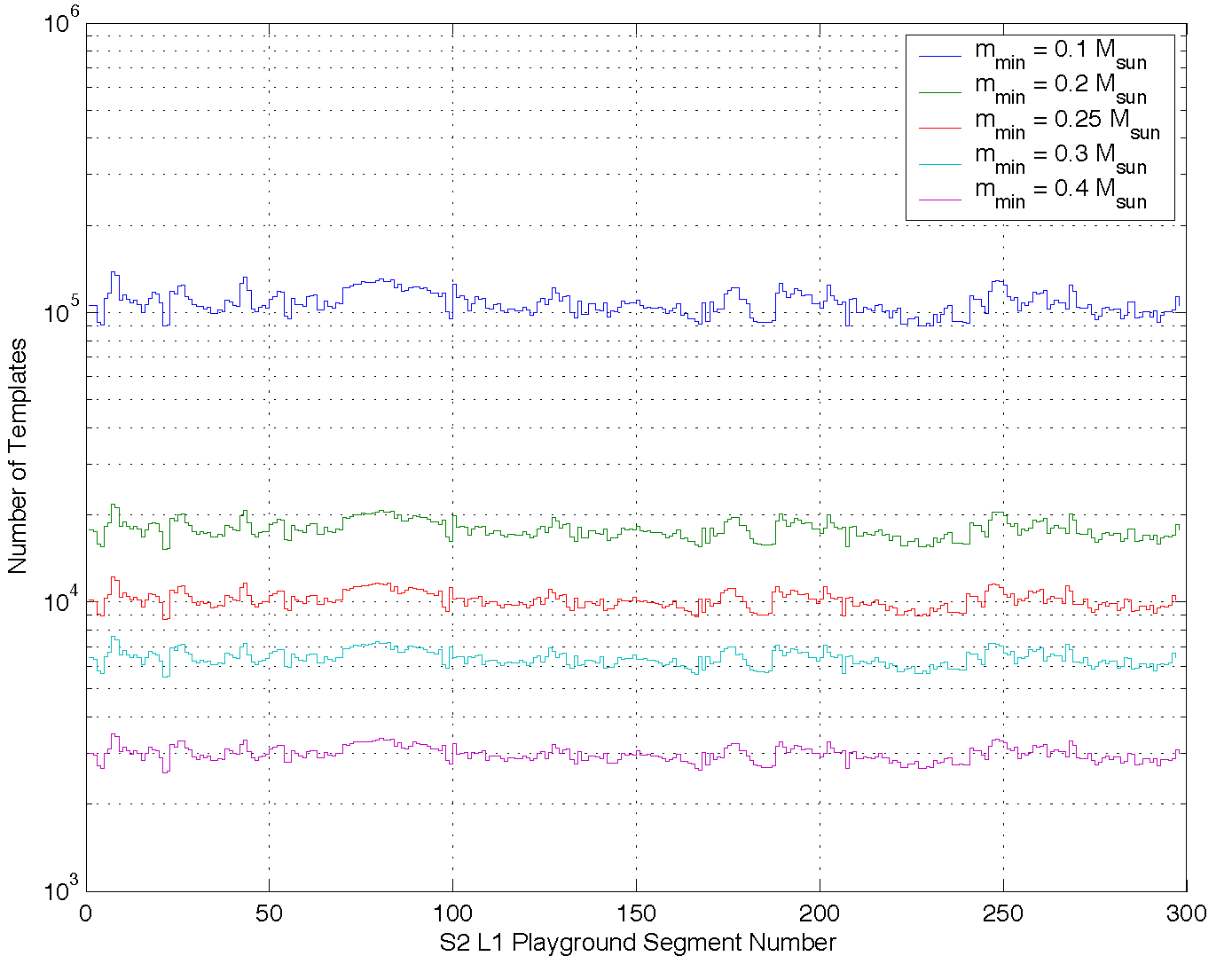
Figure 2: The plot shows the size of the template bank, generated with a minimal match of $97\%$, for various values of $m_{\mathrm{min}}$. As described in section 5.3.1 the size of the template bank is proportional to $m_{\mathrm{min}}^{-8/3}$, where $m_{\mathrm{min}}$ is the mass parameter of the smallest equal mass binary in the template bank. Using these data, it was decided that the lowest mass accessible was $m_{\mathrm{min}}=0.2\,M_{\odot}$, given the available computational resources.

Figure 2 shows the effect of $h_{+}$ and $h_{\times}$ on a ring of particles that lie in the $xy$ plane. We can see for the plus polarization that the effect of a gravitational wave is to stretch the ring in the $x$ direction, while squeezing it in the $y$ direction for the first half of a cycle and then squeeze in the $x$ direction and stretch in the $y$ direction for latter half of the cycle. There is therefore a relative change in length between the two particles $AB$ and $CD$ as a gravitational wave passes. The overall effect of a gravitational wave containing both polarizations propagating in the $z$ direction is

$$\delta x(t-z) =\frac{1}{2}\left[h_{+}(t-z)x_{(0)}+h_{\times}(t-z)y_{(0)}\right],$$ (2.28)

$$\delta y(t-z) =\frac{1}{2}\left[-h_{+}(t-z)y_{(0)}+h_{\times}(t-z)x_{(0)}\right].$$ (2.29)

It is the change in the distance between a pair of particles that we attempt to measure with gravitational wave detectors. We can see from equation (2.29) that the change in length is proportional to the original distance between the test masses. For a pair of test masses separated by a length $L$, we define the gravitational wave strain $h$ to be the fractional change in length between the masses

$$h\equiv\frac{1}{2}\frac{\Delta L}{L}.$$ (2.30)

The reason to include a factor of $1/2$ in this definition will become apparent when we discuss measuring gravitational wave strain with an interferometer.

2.2 The LIGO Gravitational Wave Detectors

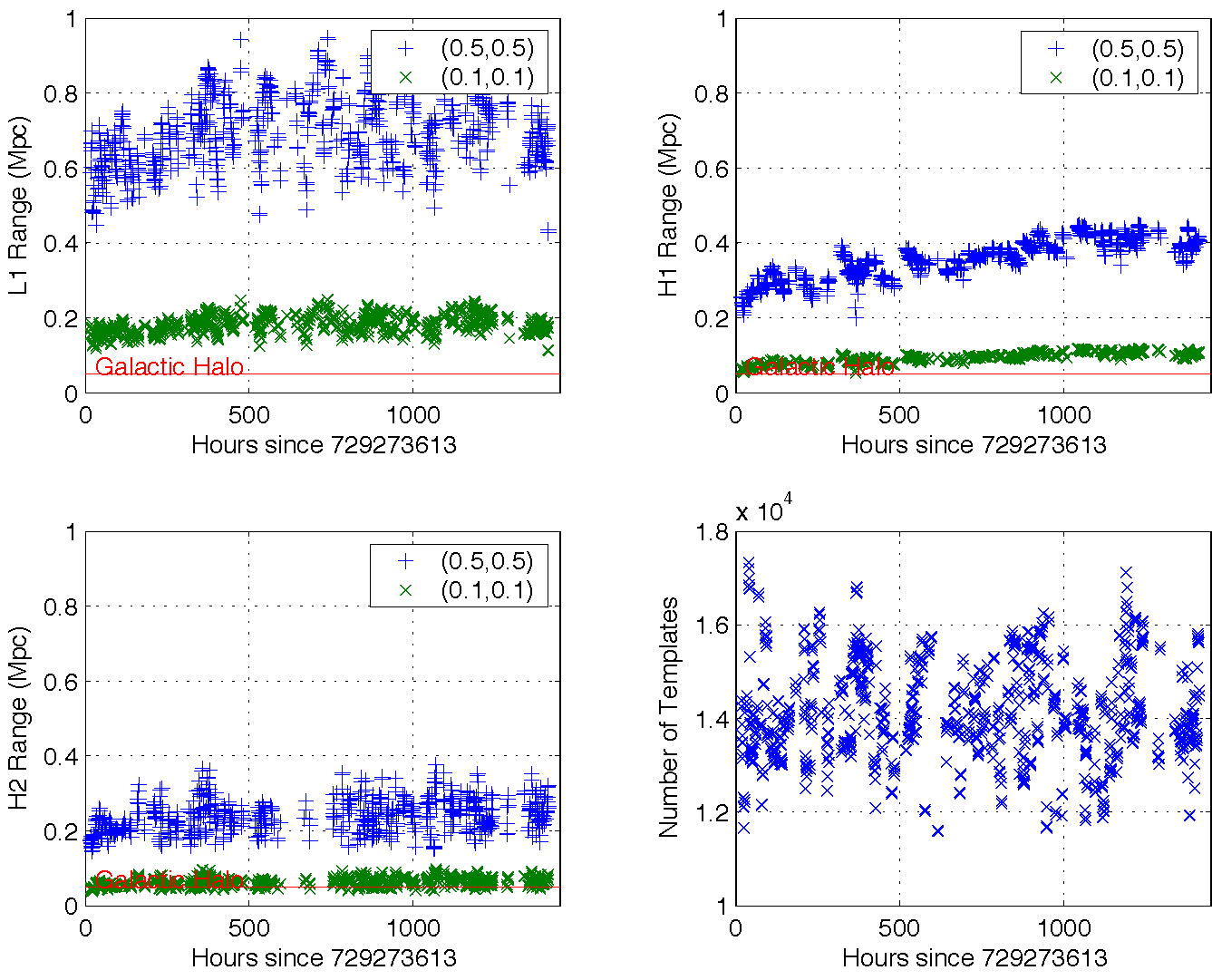
Figure 3: The bottom right plot shows the variation in the size of the MACHO search template bank over the course of the S2 run. As described in the text, the template bank is generated using L1 data to cover a region of parameter space from $0.2\,M_{\odot}$ to $1.0\,M_{\odot}$ (component mass) at $95\%$ minimal match. This template bank is used to filter the L1 data in the triggered search pipeline. The other three plots show the variation in distance to which the three LIGO interferometers can see an optimally oriented binary at signal-to-noise ratio 8 over the S2 run. Since this is a function of the masses of the binary, this range is shown for a $(0.1,0.1)\,M_{\odot}$ and a $(0.5,0.5)\,M_{\odot}$ binary.

Several major efforts are underway[Barish:1999, Acernese:2002, Luck:1997hv] to measure the strain produced by a gravitational wave using laser interferometry. The results in this thesis are based on data from the Laser Interferometer Gravitational wave Observatory (LIGO). LIGO operates three power-recycled-Fabry-Perot-Michelson interferometers in the United States. Two of these are co-located at the LIGO Hanford Observatory, WA (LHO) and one at the LIGO Livingston Observatory (LLO). The interferometers at LHO are 4 km and 2 km in arm length and are referred to as H1 and H2, respectively. The interferometer at LLO is a 4 km long interferometer referred to as L1. The locations and names of the detectors are shown in figure 3. As we saw in chapter 1, to detect the gravitational wave strain produced by typical astrophysical sources we need to measure $h\sim 10^{-22}$. If we separate our test masses by a distance of $4$ km (a practical distance for earthbound observatories) the challenge faced by gravitational wave astronomers is to measure changes of length of order

$$\Delta L\sim 10^{-22}\times 10^{4}\,\mathrm{m}\sim 10^{-18}\,\mathrm{m}.$$ (2.31)

2.2.1 The Design of the LIGO Interferometers

In an interferometric gravitational wave detector the freely falling masses described in the previous section are the mirrors that form the arms of the interferometer and laser light is used to measure the change in length between the mirrors. The challenge facing experimenters constructing a gravitational wave interferometer is to measure changes of length of order $\sim 10^{-18}\,\mathrm{m}$ using laser light has a wavelength of $\lambda_{l}\sim 10^{-6}$ m. It should be noted that measuring a phase shift

$$\Delta\Phi\sim\frac{\Delta L}{\lambda_{l}}\sim 10^{-12}$$ (2.32)

is a factor $10^{12}$ more sensitive than the interferometers used by Michelson and Morely to disprove the existence of the ether.

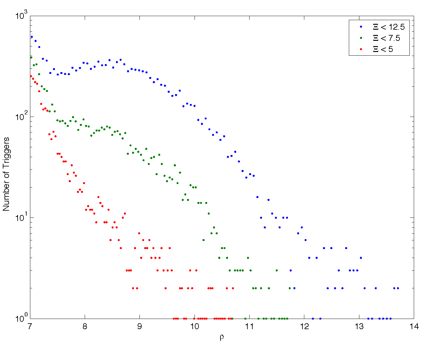
Figure 4: The figure shows a histogram of all the triggers generated from the H1 data using the triggered search (i.e. no coincidence with L1 or H2 has been applied to the triggers). The signal-to-noise threshold is $\rho_{\ast}=7$ and the parameters of the $\chi^{2}$ veto are $p=15,\delta^{2}=0.04,\Xi=12.5$, as in the S2 binary neutron star search. If the interferometer data is Gaussian, then we would expect the histogram to be monotonically decreasing with increasing signal-to-noise ratio; however, there is a pronounced “hump” in the histogram at $\rho\approx 9$ suggesting some non-Gaussian feature in the data. By lowering the value of $\Xi$ to $5$, we can remove this feature from the histogram, but we must be careful in doing so that we do not reduce the detection efficiency of the pipeline.

A schematic of a simple Michelson interferometer is illustrated in figure 4 (a). Laser light is shone on a beam splitter which reflects half the light into the $x$-arm and transmits half the light into the $y$-arm of the interferometer. The light travels a distance $L$ in each arm and then is reflected back towards the beam splitter by the end test masses. These masses are equivalent to the test masses $B$ and $D$ in section 2.1. Consider the light in the $x$-arm. For the laser light, the spacetime interval between the beam splitter and the end test mass is given by

$$ds^{2}=g_{\mu\nu}\,dx^{\mu}\,dx^{\nu}=0.$$ (2.33)

In the presence of a plus polarized, sinusoidal, gravitational wave traveling in the $z$-direction, equation (2.33) becomes

$$c^{2}dt^{2}=\left[1+h_{+}(t-z)\right]dx^{2}+\left[1-h_{+}(t-z)\right]dy^{2}+dz^{2}.$$ (2.34)

We can measure the response of the interferometer to a gravitational wave by considering the phase shift of light in the arms. The phase that the light acquires propagating from the beam splitter to the $x$-end test mass and back is given by[Saulson:1994]

$$\begin{split}\Phi_{x}&=\int_{0}^{\tau_{\mathrm{RT}}}2\pi f_{l}\,dt\\ &=\frac{1}{c}\int_{0}^{L}2\pi f_{l}\sqrt{1+h_{+}}\,dx-\frac{1}{c}\int_{L}^{0}2\pi f_{l}\sqrt{1+h_{+}}\,dx\\ &\approx\frac{4\pi f_{l}L}{c}\left(1+\frac{h_{+}}{2}\right),\end{split}$$ (2.35)

where $\tau_{\mathrm{RT}}$ is the round trip time of the light and $f_{l}$ is its frequency. We have discarded higher order terms in $h_{+}$ as their effect is negligible. We can see that the phase shift acquired in the $x$-arm due to the gravitational wave is

$$\delta\Phi_{x}=\frac{2\pi}{\lambda_{l}}h_{+}L.$$ (2.36)

A similar calculation shows that the phase shift acquired in the $y$-arm is

$$\delta\Phi_{y}=-\frac{2\pi}{\lambda_{l}}h_{+}L$$ (2.37)

and so the difference in phase shift between the arms is

$$\Delta\Phi=\frac{4\pi}{\lambda_{l}}h_{+}L.$$ (2.38)

A typical astrophysical source of gravitational radiation of interest to LIGO, has a frequency $f_{\mathrm{GW}}\sim 100$ Hz. Therefore the wavelength of the gravitational wave is $\lambda_{\mathrm{GW}}\sim 3000$ km. If $\tau_{\mathrm{RT}}=1/f_{\mathrm{GW}}$ there will be no phase shift of the light at leading order in $h_{+}$. The light spends exactly one gravitational wave period in the arm and so the phase shift acquired by positive values of $h_{+}(t-z)$ is canceled out by the phase shift due to negative values of $h_{+}(t-z)$. The interferometer achieves maximum sensitivity when the light spends half a gravitational wave period in the arms, that is

$$L=\frac{\lambda_{\mathrm{GW}}}{2}\sim 1000\,\mathrm{km}$$ (2.39)

which is a hopelessly impractical length for a earthbound detector. Instead, a simple Michelson interferometer is enhanced by placing two additional mirrors in the arms of the interferometer near the beam splitter, as shown in figure 4 (b). These inner $x$ and $y$ test masses (referred to as ITMX and ITMY) are designed in LIGO to store the light in the arms for approximately one half of a gravitational wave period. The mirrors create a Fabry-Perot cavity in each arm that stores the light for $B\sim 200$ bounces, giving a phase shift of

$$\Delta\Phi=4\pi\frac{L}{\lambda_{l}}Bh_{+}\sim 10\times\frac{4\times 10^{3}\,\mathrm{m}}{10^{-6}\,\mathrm{m}}\times 200\times h_{+}.$$ (2.40)

For a gravitational wave strain of $h\sim 10^{-22}$, this increases $\Delta\Phi$ by 3 orders of magnitude to a phase shift $\Delta\Phi\sim 10^{-9}$. Further increasing $B$ does not gain additional sensitivity, however, as storing the light for longer than half a gravitational wave period causes it to lose phase shift as the sign of the gravitational wave strain changes.

Is it possible to measure a phase shift of $10^{-9}$ using a Fabry-Perot-Michelson interferometer? We measure the phase shift by averaging the light at the photodiode over some period, $\tau$. Let $N$ be the number of photons from the laser arriving at the photodiode in the time $\tau$. The measured number of photons in the averaging interval is a Poisson process, with probability distribution function for $N$ given by

$$p(N)=\frac{\bar{N}^{N}\exp\left(-\bar{N}\right)}{N!},$$ (2.41)

where $\bar{N}$ is the mean number of photons per interval $\tau$. The $1\sigma$ uncertainty in the number of photons arriving in the averaging time is therefore

$$\Delta N=\sqrt{\bar{N}}.$$ (2.42)

The accuracy to which we can measure the phase shift for a given input laser power is constrained by the uncertainty principle,

$$\Delta t\,\Delta E\geq\frac{\hbar}{2}$$ (2.43)

as follows. The energy of the light arriving at the photodiode in time $\tau$ is

$$E=\hbar\frac{2\pi c}{\lambda_{l}}N,$$ (2.44)

which, due to the counting of photons, has uncertainty

$$\Delta E=\hbar\frac{2\pi c}{\lambda_{l}}\sqrt{\bar{N}}.$$ (2.45)

The uncertainty in the measured the phase is related to the uncertainty in the time that a wavefront reaches the beam splitter , i.e.

$$\Delta\Phi=2\pi c\frac{\Delta t}{\lambda_{l}}$$ (2.46)

Substituting equation (2.45) and (2.46) into equation (2.43), we obtain

$$\Delta t\,\Delta E=\frac{\Delta\Phi\lambda_{l}}{2\pi c}\hbar\frac{2\pi c}{\lambda_{l}}\sqrt{\bar{N}}\geq\frac{\hbar}{2}.$$ (2.47)

The accuracy which which we can measure the phase is therefore no better than

$$\Delta\Phi\geq\frac{1}{\sqrt{\bar{N}}}.$$ (2.48)

Hence photon counting statistics limits the accuracy with which the phase shift can be measured by this method, and this equation tells us how many photons we need in an averaging period to measure a given phase shift. We need at least

$$N\geq\frac{1}{2\left(\Delta\Phi\right)^{2}}$$ (2.49)

photons to measure the phase shift. The optimal averaging time for a gravitational wave with frequency $f_{\mathrm{GW}}$ is half a period so that the light acquires the maximum phase shift, that is

$$\tau\approx\frac{1}{2f_{\mathrm{GW}}}.$$ (2.50)

The intensity of laser light required to measure a phase shift of $10^{-9}$ for a gravitational wave of $f_{\mathrm{GW}}\sim 100$ Hz is then

$$\begin{split}I&=N\left(\frac{2\pi\hbar c}{\lambda_{l}}\right)\left(\frac{1}{2f_{\mathrm{GW}}}\right)^{-1}\\ &=\left(\frac{1}{\Delta\Phi}\right)^{2}\left(\frac{2\pi\hbar c}{\lambda_{l}}\right)2f_{\mathrm{GW}}\\ &\sim\left(\frac{1}{10^{-9}}\right)^{2}\left(\frac{10^{2}\times 10^{-34}\times 10^{8}}{10^{-6}}\right)10^{2}\sim 10^{2}\,\mathrm{W},\end{split}$$ (2.51)

however, lasers used in the first generation of interferometers have a typical output power of $\sim 5$ W. To increase the power in the interferometer, the final enhancement to the basic design of our interferometer is the addition of a power recycling mirror (RM) between the beam splitter and the laser, as shown in figure 4 (c). This mirror reflects some of the (otherwise wasted) laser light back into the interferometer and increases the power incident on the beam splitter so that the phase shift due to a gravitational wave of order $h\sim 10^{-23}$ can be measured.

The laser light must be resonant in the power recycling and Fabry-Perot cavities, to achieve the required power build up in the interferometer. This requires a complicated length sensing and control system[Fritschel:2001] which continuously monitors the positions of the mirrors in the interferometer and applies feedback motions via electromagnetic actuators. The interferometer is said to be locked when the control system achieves a stable resonance. The optics and the servo loop that controls their positions form the core systems of the interferometer; however the many subtleties involved in the design and operation of these detectors are outside the scope of this thesis.

2.2.2 Noise sources in an Interferometer

In reality, there are many sources of noise which can result in an apparent phase shift of the laser light. We define the interferometer strain signal, $s$, to be the relative change in the lengths of the two arms of the interferometer

$$s(t)=\frac{\Delta L_{x}-\Delta L_{y}}{L}.$$ (2.52)

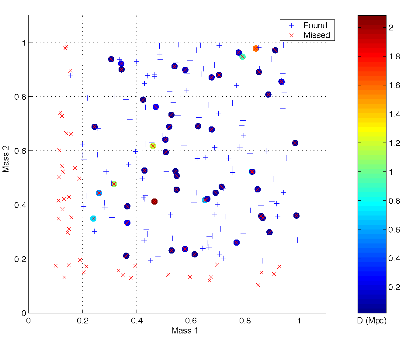
Figure 5: The figure shows the results of a small Monte Carlo simulation used to test the detection efficiency of the pipeline using H1 triggers (i.e. no coincidence with L1 or H2 has been applied to the triggers). The signal-to-noise threshold is $\rho_{\ast}=7$ and the parameters of the $\chi^{2}$ veto are $p=15,\delta^{2}=0.04,\Xi=12.5$. Found injections are shown with a $+$, missed injections are shown with a $\times$ and the masses of the injection are shown as the $x$ and $y$ coordinates. We would expect to miss any injections with a mass component below $0.2\,M_{\odot}$ due to the coverage of the template bank; however injections in the region inside the bank should be detected, unless they are at an effective distance larger than the range of the interferometer. The missed injections that we would expect to find are color coded according to the effective distance at which they are injected. Several injections are missed as they are at a large effective distance (e.g. the injection at $(0.48,0.42)\,M_{\odot}$); however there are may missed injections at distances $<200$ kpc which should be detectable in the H1 data (e.g. the injection at $(0.88,0.91)\,M_{\odot}$). Investigation of the missed injections showed they had large values of signal-to-noise ratio, but were vetoed by the $\chi^{2}$ test. This suggests that the search parameters used must be re-tuned to increase the detection efficiency.

This signal has two major additive components: (i) a gravitational wave signal $h(t)$ and (ii) all other noise sources $n(t)$. The task of gravitational wave data analysts is to search for astrophysical signals hidden in this data. The primary goal of the experimenters engaged in commissioning the LIGO detectors is the reduction of the noise appearing in $s(t)$. The noise in interferometers is measured as the amplitude spectral density $\tilde{h}(f)$. This is the square root of the power spectral density of the interferometer strain in the absence of gravitational wave signals. Figure 5 shows the target noise spectral density of the initial LIGO detectors. There are three fundamental noise sources that limit the sensitivity of these detectors:

1. Seismic noise. This is the dominant noise at low frequencies, $f\lesssim 40$ Hz. Seismic motion of the earth couples through the suspensions of the mirrors and causes them to move. To mitigate this, a system of coupled oscillators is used to isolate the mirror from the ground motion.

2. Suspension thermal noise. This noise source limits the sensitivity of the interferometer in the range $40$ Hz $\lesssim f\lesssim 200$ Hz. The steel wire suspending the mirror is at room temperature and thermal motion of the particles in the wire produce motion of the mirror and change the arm length.

3. Photon shot noise. At high frequencies, $f\gtrsim 200$ Hz, the noise is dominated by the shot noise due to the photon counting statistics discussed in the previous section.

For a detailed review of the noise sources present in LIGO’s kilometer scale interferometers, we refer the reader to [Adhikari:thesis].

2.2.3 Calibration of the Data

We do not directly record the interferometer strain $s(t)$ but rather the error signal $v(t)$ of the feedback loop used to control the differential lengths of the arms. This signal, designated LSC-AS_Q in LIGO, contains the gravitational wave signal along with other noise. The interferometer strain is reconstructed from the error signal in the frequency domain by calibrating $v(t)$ using the response function $R(f)$ of the instrument:

$$\tilde{s}(f)=R(f)\tilde{v}(f).$$ (2.53)

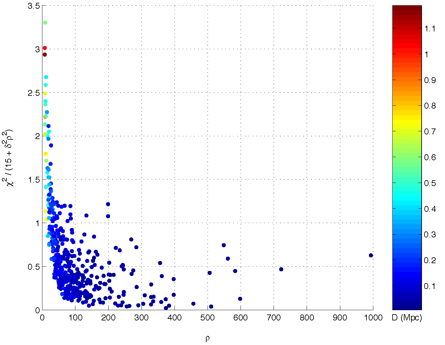
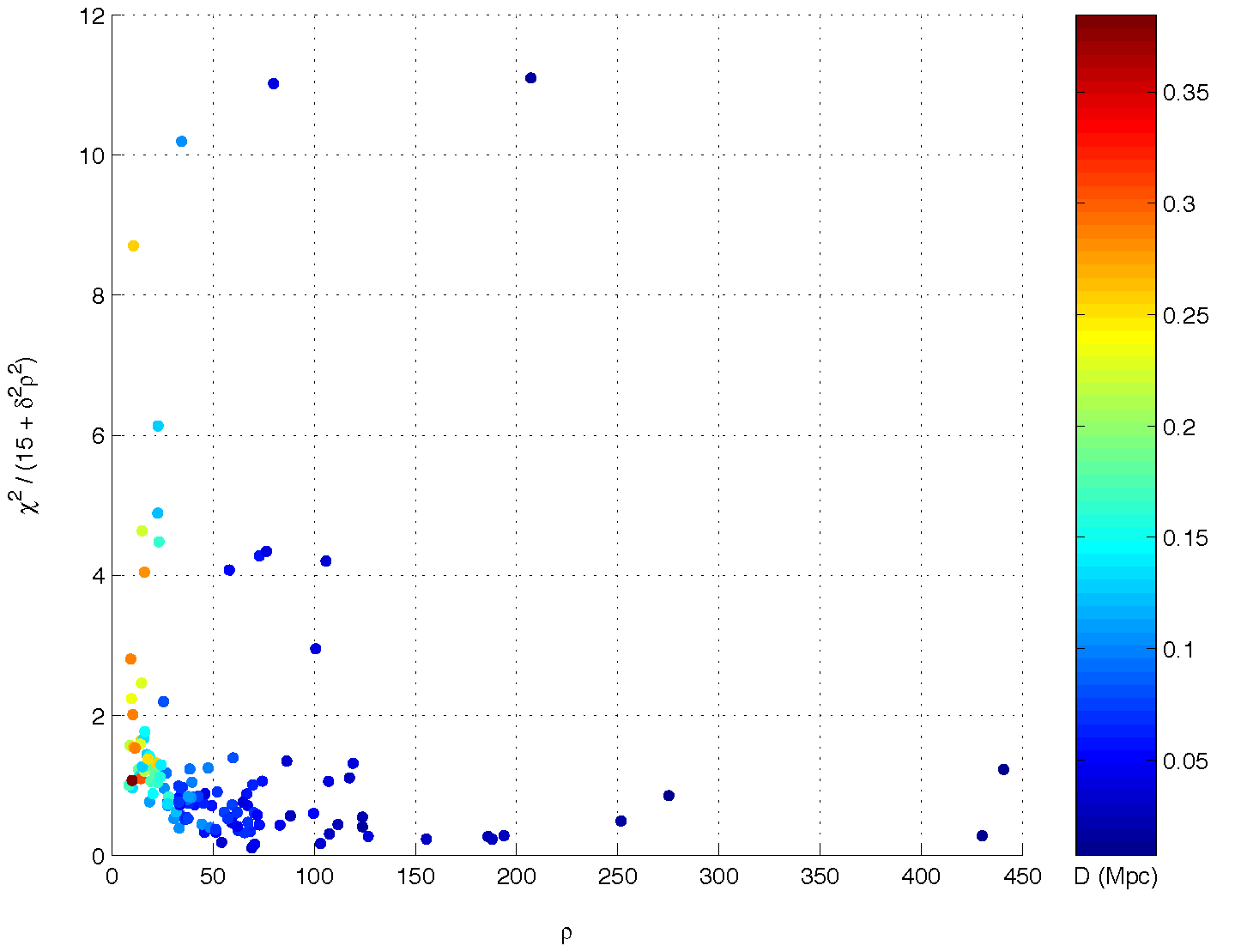
Figure 6: The plots in this figure show the values of $\rho$ and $\Xi=\chi^{2}/(15+\delta^{2}\rho^{2})$ for the inspiral triggers corresponding to injected signals found by the triggered search pipeline. The upper plot shows L1 triggers and the lower plot shows H1 triggers (which correspond to the found injections of figure 5). No coincidence has been applied to the H1 triggers at this stage; however they are generated using template banks produced from L1 triggers. The color of each trigger shows the effective distance at which it was injected. Both plots are generated with a signal-to-noise threshold of $\rho_{\ast}=7$, and the parameters of the $\chi^{2}$ veto were $p=15,\delta^{2}=0.04$ and $\Xi_{\mathrm{L1}}=12.5,\Xi_{\mathrm{L1}}=5.0$, values chosen based on the tuning of the S2 binary neutron star search. It can be seen that, at a given signal-to-noise ratio, the H1 triggers typically have higher values of $\Xi$ than the L1 triggers. This is due to the a larger mismatch between the injected signal and the templates in the H1 triggered bank.

The response function depends on three elements of the feedback control loop shown in figure 6: the sensing function $C(f)$; the actuation function $A(f)$; the digital feedback filter $D(f)$[Gonzalez:2002].

The sensing function $C(f)$ measures the response of the arm cavities to gravitational waves. It depends on the light power in the arms, which changes over time as the alignment of the mirrors change. The actuation function $A(f)$ encodes the distance the mirrors move for the applied voltage at the electromagnets. The dominant contribution to this is the pendulum response of the suspended mirrors. The digital filter $D(f)$ converts the error signal $v(t)$ into a control signal that is sent as actuation to the mirrors to keep the cavities resonant.

If $\tilde{g}(f)$ is the Fourier transform of the control signal applied to the mirrors, then the residual motion of the mirrors is given by

$$\tilde{r}(f)=\tilde{s}(f)-A(f)\tilde{g}(f)$$ (2.54)

as seen in figure 6. The corresponding error signal is

$$\tilde{v}(f)=C(f)\tilde{r}(f)$$ (2.55)

and following around the servo control loop we obtain

$$\tilde{g}(f)=D(f)\tilde{v}(f)=D(f)C(f)\tilde{r}(f).$$ (2.56)

Substituting equation (2.56) into equation (2.54) and solving for $\tilde{r}(f)$, we obtain

$$\tilde{r}(f)=\frac{\tilde{s}(f)}{1+A(f)D(f)C(f)}=\frac{\tilde{s}(f)}{1+G(f)},$$ (2.57)

where $G(f)$ is the open loop gain of the interferometer, defined by $G(f)=A(f)D(f)C(f)$. The error signal is then

$$\tilde{v}(f)=C(f)\tilde{r}(f)=\tilde{s}(f)\frac{C(f)}{1+G(f)}$$ (2.58)

and hence

$$R(f)=\frac{1+G(f)}{C(f)}.$$ (2.59)

The value of the digital filter $D(f)$ is a known at all times. The actuation function can be measured by configuring the interferometer as a simple Michelson, driving a mirror and counting the number of fringes that appear at the photodiode for a given applied signal. This provides a measure of the displacement of the mirror for a given control signal. Since $A(f)$ is due to the pendulum response of the mirror and known filters used in the electronics that drive the motion of the mirror, it does not change and its value can be established before data taking. A sinusoidal signal of known amplitude that sweeps up in frequency is added to the control signal after the interferometer is brought into resonance. By comparing the amplitude of this calibration sweep in the output of the detector to the known input, the value of the open loop gain and (and hence the sensing function) can be determined as a function of frequency. The values of the sensing function and open loop gain at the time of calibration are denoted $C_{0}(f)$ and $G_{0}(f)$.

Although the LIGO detectors have an alignment control system that tries to keep the power in the arms constant, the power in the cavity can still change significantly over the course of data taking. These fluctuations in power mean that the sensing function can change on time scales of order minutes or hours. To measure $C(f)$ during data taking sinusoidal signals of known amplitude and frequency $f_{\mathrm{cal}}$ added to the control signals that drive the mirrors. These calibration signals show up as peaks in the spectrum and are called calibration lines. By measuring the amplitude of a calibration line over the course of the run compared to the time at which the calibration sweep was taken, we may measure the change in the sensing function

$$C(f;t)=\alpha(t)C_{0}(f),$$ (2.60)

where $\alpha(t)$ is the ratio of the calibration line amplitude at time $t$ to the reference time. We also allow the digital gain of the feedback loop to vary by a known factor $\beta(t)$ so

$$D(f;t)=\beta(t)D_{0}(f).$$ (2.61)

The response function at any given time, $t$, becomes

$$R(f;t)=\frac{1+\alpha(t)\beta(t)G_{0}(f)}{\alpha(t)C_{0}(f)}.$$ (2.62)

To analyze the interferometer data we therefore need the error signal, $v(t)$, which contains the gravitational wave signal, the functions $C_{0}(f)$ and $G_{0}(f)$, which contain the reference calibration, and the values of $\alpha(t)$ and $\beta(t)$, which allow us to properly calibrate the data.

2.3 Gravitational Waves from Binary Inspiral

Consider a circular binary system comprised of two black holes $m_{1},m_{2}\sim M_{\odot}$, separated by a distance $a$. If $a\gg 2GM/c^{2}$, where $M=m_{1}+m_{2}$, then Newtonian gravity will provide a reasonably accurate description of the binary dynamics. If we neglect higher order multipoles, the gravitational wave field is determined by the quadrupole formula[MTW73]

$$h_{jk}^{\mathrm{TT}}=\frac{2G}{c^{4}r}\frac{d^{2}\mathcal{I}_{jk}^{\mathrm{TT}}(t-r)}{dt^{2}},$$ (2.63)

where $\mathcal{I}_{jk}$ is the quadrupole moment of the binary, defined by

$$\mathcal{I}_{jk}=\int\rho(\boldsymbol{x})x_{j}x_{k}\,d^{3}x$$ (2.64)

and $\mathcal{I}_{jk}^{\mathrm{TT}}$ is the transverse traceless part of of $\mathcal{I}_{jk}$. Since the binary can be described by Newtonian theory, Kepler’s laws are satisfied and the orbital angular velocity is

$$\Omega=\sqrt{\frac{GM}{a^{3}}}.$$ (2.65)

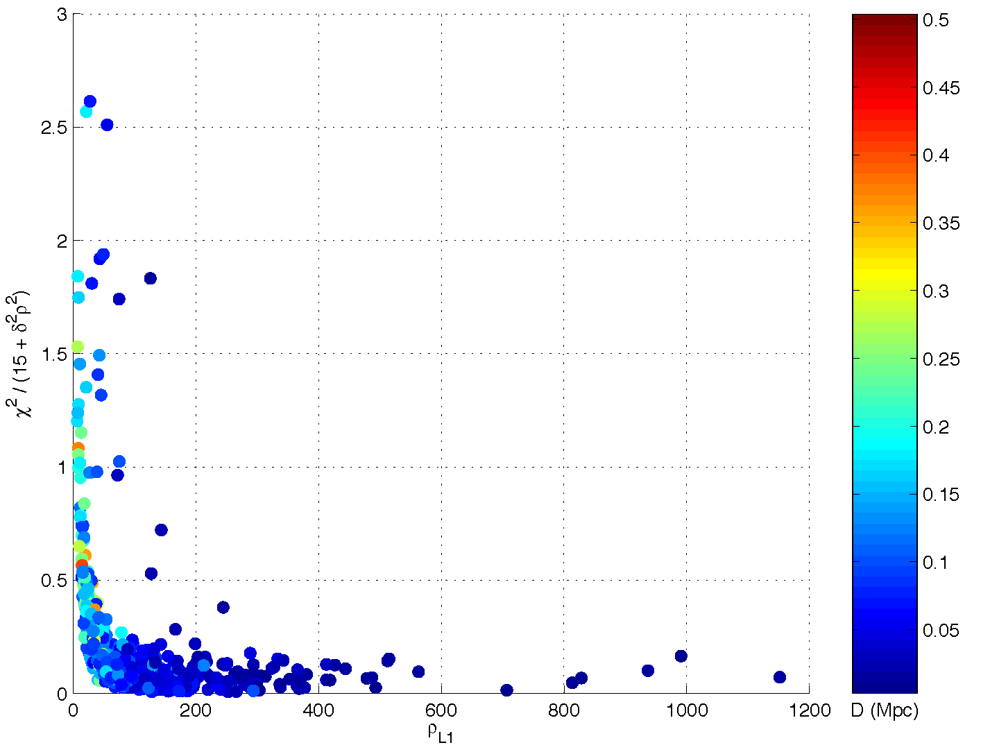
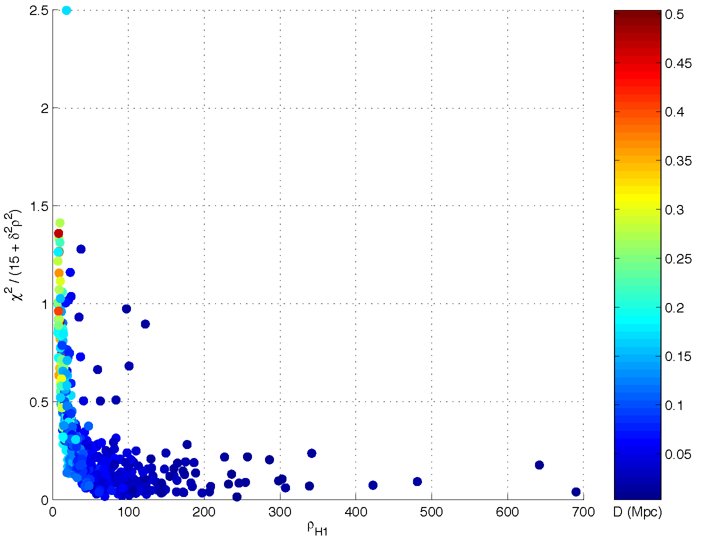
Figure 7: The plots in this figure should show the observed values of $\rho$ and $\Xi=\chi^{2}/(15+\delta^{2}\rho^{2})$ for the inspiral triggers corresponding to injected signals found by the triggered search pipeline using the final set of parameters chosen. The upper plot shows L1 triggers and the lower plot shows H1 triggers. No coincidence has been applied to the H1 triggers at this stage; however they are generated using template banks produced from L1 triggers. These plots should be compared to those shown in figure 6. By tuning the value of $\delta^{2}$ to $0.2$, it can be seen that much lower values of $\Xi$ are obtained for the H1 injections. This suggests that we could further reduce the threshold $\Xi_{\ast}$, although this was not done as no coincident triggers were found in the playground data and a looser value of $\delta$ allowed us to probe the region slightly outside the template bank parameter space.

In a Cartesian coordinate system $(x,y,z)$ with origin at the center of mass of the binary as shown in figure 7, the mass distribution of the binary is given, in the point mass approximation, by

$$\begin{split}\rho(\boldsymbol{x})&=m_{1}\left[\delta(x-r_{1}\cos\Omega t)\delta(y-r_{1}\sin\Omega t)\delta(z)\right]\\ &\quad+m_{2}\left[\delta(x+r_{2}\cos\Omega t)\delta(y+r_{2}\sin\Omega t)\delta(z)\right],\end{split}$$ (2.66)

where

$$r_{1} =\frac{m_{2}}{m_{1}+m_{2}}a,$$ (2.67)

$$r_{2} =\frac{m_{1}}{m_{1}+m_{2}}a.$$ (2.68)

Introduce a second, spherical polar coordinate system labeled $(r,\iota,\phi_{0})$ related to the Cartesian coordinate system by

$$\boldsymbol{e}_{\hat{\iota}} =\cos\iota\cos\phi_{0}\boldsymbol{e}_{\hat{x}}+\cos\iota\sin\phi_{0}\boldsymbol{e}_{\hat{y}}-\sin\iota\boldsymbol{e}_{\hat{z}},$$ (2.69)

$$\boldsymbol{e}_{\hat{\phi}_{c}} =-\sin\phi_{0}\boldsymbol{e}_{\hat{x}}+\cos\phi_{0}\boldsymbol{e}_{\hat{y}}.$$ (2.70)

To calculate the gravitational radiation $h_{jk}^{\mathrm{TT}}$ seen by an observer at a position $(r,\iota,\phi_{0})$ relative to the center of mass of the binary we first calculate the quadrupole moment of the mass distribution in the frame of the binary. The non-zero components of $\mathcal{I}_{jk}$ are $\mathcal{I}_{xx}$, $\mathcal{I}_{yy}$ and $\mathcal{I}_{xy}=\mathcal{I}_{yx}$. The detailed derivation of $\mathcal{I}_{xx}$ following from equation (2.64) gives

$$\begin{split}\mathcal{I}_{xx}&=\int m_{1}\left[\delta(x-r_{1}\cos\Omega t)\delta(y-r_{1}\sin\Omega t)\delta(z)\right]\\ &\quad+m_{2}\left[\delta(x+r_{2}\cos\Omega t)\delta(y+r_{2}\sin\Omega t)\delta(z)\right]x^{2}\,d^{3}x\\ &=(m_{1}r_{1}^{2}+m_{2}r_{2}^{2})\cos^{2}\Omega t\\ &=\left[m_{1}\left(\frac{m_{2}}{m_{1}+m_{2}}\right)^{2}+m_{2}\left(\frac{m_{1}}{m_{1}+m_{2}}\right)^{2}\right]a^{2}\cos^{2}\Omega t\\ &=\left(\frac{m_{1}m_{2}^{2}+m_{2}m_{1}^{2}}{(m_{1}+m_{2})^{2}}\right)a^{2}\cos^{2}\Omega t\\ &=\left(\frac{m_{1}m_{2}(m_{1}+m_{2})}{(m_{1}+m_{2})^{2}}\right)a^{2}\cos^{2}\Omega t\\ &=\mu a^{2}\cos^{2}\Omega t\\ &=\frac{1}{2}\mu a^{2}\left(1+\cos 2\Omega t\right).\end{split}$$ (2.71)

Here

$$\mu=\frac{m_{1}m_{2}}{m_{1}+m_{2}}$$ (2.72)

is the reduced mass of the binary and we have used

$$\begin{split}\int\delta(x-x_{0})f(x)\,d^{3}x&=f(x_{0}),\\ \int\delta(x)\,d^{3}x=1.\end{split}$$ (2.73)

The other components are derived in a similar way to give

$$\mathcal{I}_{yy}=\frac{1}{2}\mu a^{2}\left(1-\cos 2\Omega t\right)$$ (2.74)

and

$$\mathcal{I}_{xy}=\mathcal{I}_{yx}=\frac{1}{2}\mu a^{2}\sin 2\Omega t.$$ (2.75)

The second time derivative of the quadrupole moment is then

$$\ddot{\mathcal{I}}_{xx} =-2\mu a^{2}\Omega^{2}\cos 2\Omega t$$ (2.76)

$$\ddot{\mathcal{I}}_{yy} =2\mu a^{2}\Omega^{2}\cos 2\Omega t$$ (2.77)

$$\ddot{\mathcal{I}}_{xy} =\ddot{\mathcal{I}}_{yx}=-2\mu a^{2}\Omega^{2}\sin 2\Omega t$$ (2.78)

in the frame of the binary. We transform these to the frame of the observer using the standard relations

$$A^{\prime}_{ij} =\frac{\partial x_{k}}{\partial x_{i}^{\prime}}\frac{\partial x_{l}}{\partial x_{j}^{\prime}}A_{kl}$$ (2.79)

$$\hat{\boldsymbol{e}}_{i}^{\prime} =\frac{\partial x_{j}}{\partial x_{i}^{\prime}}\hat{\boldsymbol{e}}_{j}$$ (2.80)

to obtain

$$\begin{split}\ddot{\mathcal{I}}_{\iota\iota}&=\ddot{\mathcal{I}}_{xx}\cos^{2}\iota\cos^{2}\phi_{0}+\ddot{\mathcal{I}}_{yy}\cos^{2}\iota\sin^{2}\phi_{0}+2\ddot{\mathcal{I}}_{xy}\cos^{2}\iota\sin\phi_{0}\cos\phi_{0}\\ &=-2\mu a^{2}\Omega^{2}\cos(2\Omega t)\cos^{2}\iota\cos 2\phi_{0}-2\mu a^{2}\Omega^{2}\sin(2\Omega t)\cos^{2}\iota\sin 2\phi_{0}\\ &=-2\mu a^{2}\Omega^{2}\cos^{2}\iota\cos\left(2\Omega t-2\phi_{0}\right).\end{split}$$ (2.81)

Similar transformations give the other components of $\ddot{\mathcal{I}}_{jk}$

$$\ddot{\mathcal{I}}_{\phi_{0}\phi_{0}} =2\mu a^{2}\Omega^{2}\cos(2\Omega t)\cos 2\phi_{0}+\frac{1}{2}\mu a^{2}\Omega^{2}\sin(2\Omega t)\sin 2\phi_{0}$$

$$=2\mu a^{2}\Omega^{2}\cos\left(2\Omega t-2\phi_{0}\right),$$ (2.82)

$$\ddot{\mathcal{I}}_{\iota\phi_{0}}=\ddot{\mathcal{I}}_{\phi_{0}\iota} =-2\mu a^{2}\Omega^{2}\cos\iota\sin\left(2\Omega t-2\phi_{0}\right).$$ (2.83)

Since these are the transverse components of $\ddot{\mathcal{I}}_{ij}$, we can simply remove their trace to obtain $\ddot{\mathcal{I}}_{ij}^{\mathrm{TT}}$:

$$\begin{split}\ddot{\mathcal{I}}_{\iota\iota}^{\mathrm{TT}}=-\ddot{\mathcal{I}}_{\phi_{0}\phi_{0}}^{\mathrm{TT}}&=\ddot{\mathcal{I}}_{\iota\iota}-\frac{1}{2}\left(\ddot{\mathcal{I}}_{\iota\iota}+\ddot{\mathcal{I}}_{\phi_{0}\phi_{0}}\right)=\frac{1}{2}\left(\ddot{\mathcal{I}}_{\iota\iota}-\ddot{\mathcal{I}}_{\phi_{0}\phi_{0}}\right)\\ &=-\mu a^{2}\Omega^{2}\left(1+\cos^{2}\iota\right)\cos\left(2\Omega t-2\phi_{0}\right),\\ \ddot{\mathcal{I}}_{\iota\phi_{0}}^{\mathrm{TT}}=\ddot{\mathcal{I}}_{\phi_{0}\iota}^{\mathrm{TT}}&=2\mu a^{2}\Omega^{2}\cos\iota\sin(2\Omega t-2\phi_{0})\end{split}$$ (2.84)

It is now a simple matter to compute the form of the gravitational radiation using the quadrupole formula in equation (2.63)

$$h_{\iota\iota}^{\mathrm{TT}} =\frac{2G}{c^{4}\,r}\ddot{\mathcal{I}}_{\iota\iota}^{\mathrm{TT}}=-\frac{2G\mu a^{2}\Omega^{2}}{c^{4}\,r}(1+\cos^{2}\iota)\cos\left(2\Omega t-2\phi_{0}\right)$$ (2.85)

$$h_{\iota\phi_{0}}^{\mathrm{TT}} =\frac{2G}{c^{4}\,r}\ddot{\mathcal{I}}_{\iota\iota}^{\mathrm{TT}}=-\frac{4G\mu a^{2}\Omega^{2}}{c^{4}\,r}\cos\iota\sin\left(2\Omega t-2\phi_{0}\right).$$ (2.86)

We can further simplify these equations by using Kepler’s third law

$$a=\left(\frac{GM}{\Omega^{2}}\right)^{\frac{1}{3}}$$ (2.87)

and defining the gravitational wave frequency $f$ which is twice the orbital frequency

$$f=2\left(\frac{\Omega}{2\pi}\right).$$ (2.88)

If we use the basis vectors $\boldsymbol{e}_{\iota}$ and $\boldsymbol{e}_{\phi_{0}}$ as the polarization axes of the gravitational wave we obtain

$$h_{+}(t) =h_{\iota\iota}^{\mathrm{TT}}=-\frac{2G}{c^{4}r}\mu(\pi GMf)^{\frac{2}{3}}(1+\cos^{2}\iota)\cos(2\pi ft-2\phi_{0})$$ (2.89)

$$h_{\times}(t) =h_{\iota\phi_{0}}^{\mathrm{TT}}=-\frac{4G}{c^{4}r}\mu(\pi GMf)^{\frac{2}{3}}\cos\iota\sin(2\pi ft-2\phi_{0})$$ (2.90)

If the vector $\boldsymbol{e}_{r}$ points from the binary to our gravitational wave detector, the angles $\iota$ and $\phi_{0}$ are known as the inclination angle and the orbital phase and $r$ is the luminosity distance from the detector to the binary.

We assume that the binary evolves through a sequence of quasi-stationary circular orbits. The orbital energy for a binary with given separation, $a$, is given by the standard Newtonian formula

$$E=-\frac{1}{2}\frac{G\mu M}{a}.$$ (2.91)

The loss energy due to quadrupolar gravitational radiation is[MTW73]

$$\frac{dE}{dt}=-\frac{G}{5c^{5}}\left\langle\frac{d^{3}\mathcal{I}^{\mathrm{TT}}_{jk}}{dt^{3}}\frac{d^{3}\mathcal{I}^{\mathrm{TT}}_{jk}}{dt^{3}}\right\rangle=\frac{32G^{4}}{5c^{5}}\frac{M^{3}\mu^{2}}{a^{5}}$$ (2.92)

and so the inspiral rate for circular orbits is given by

$$\frac{da}{dt}=\frac{dE}{dt}\frac{da}{dE}=-\frac{64G^{3}}{5c^{5}}\frac{\mu M^{2}}{a^{3}}.$$ (2.93)

The evolution of $a$ as a function of time can therefore be obtained by integrating

$$a^{3}\,da =-\frac{64G^{3}}{5c^{5}}\mu M^{2}\,dt$$ (2.94)

$$\frac{a^{4}}{4} =\frac{64G^{3}}{5c^{5}}\mu M^{2}(t_{c}-t)$$ (2.95)

and so

$$a(t)=\left(\frac{256G^{3}}{5c^{5}}\mu M^{2}\right)^{\frac{1}{4}}\left(t_{c}-t\right)^{\frac{1}{4}}$$ (2.96)

which tells us that the orbit shrinks as orbital energy is lost in the form of gravitational waves. As the orbit shrinks, the orbital frequency increases and hence the gravitational wave frequency and amplitude increase. We call this type of evolution a chirp waveform. The evolution of the gravitational wave frequency $f(t)$ can be obtained by substituting Kepler’s third law, equation (2.87), into equation (2.95) to obtain

$$\begin{split}\left(GM\right)^{\frac{4}{3}}\Omega^{-\frac{8}{3}}&=\frac{256G^{3}}{5c^{5}}\mu M^{2}(t_{c}-t)\\ &=\frac{256G^{3}}{5c^{5}}\eta M^{4}\frac{(t_{c}-t)}{M},\end{split}$$ (2.97)

where we have defined $\eta=\mu/M$. From this, we may obtain

$$\Omega^{-\frac{8}{3}}=\frac{256}{c^{8}}\left(GM\right)^{\frac{8}{3}}\frac{c^{3}\eta}{5GM}(t_{c}-t).$$ (2.98)

If we define $\Theta(t)$ as the dimensionless time variable

$$\Theta(t)=\frac{c^{3}\eta}{5GM}(t_{c}-t),$$ (2.99)

then we obtain

$$\Omega^{-\frac{8}{3}}=\left(\frac{8GM}{c^{3}}\right)^{\frac{8}{3}}\Theta(t)$$ (2.100)

which written in terms of the gravitational wave frequency $f=\Omega/\pi$ is

$$f(t)=\frac{c^{3}}{8\pi GM}\left[\Theta(t)\right]^{-\frac{3}{8}}.$$ (2.101)

We define the cosine chirp $h_{c}$ and the sine chirp $h_{s}$ as

$$h_{c}(t) =\frac{2}{c^{2}}\left(\frac{\mu}{M_{\odot}}\right)\left[\pi GMf(t)\right]^{\frac{2}{3}}\cos\left[2\phi(t)-2\phi_{0}\right],$$ (2.102)

$$h_{s}(t) =\frac{2}{c^{2}}\left(\frac{\mu}{M_{\odot}}\right)\left[\pi GMf(t)\right]^{\frac{2}{3}}\sin\left[2\phi(t)-2\phi_{0}\right],$$ (2.103)

where the orbital phase $\phi(t)$ is

$$\phi(t)=2\pi\int f(t)\,dt$$ (2.104)

and $f(t)$ is given by equation (2.101). The $+$ and $\times$ waveforms are

$$h_{+}(t) =-\frac{GM_{\odot}}{c^{2}r}(1+\cos^{2}\iota)h_{c}(t),$$ (2.105)

$$h_{\times}(t) =-\frac{2GM_{\odot}}{c^{2}r}\cos\iota h_{s}(t).$$ (2.106)

If the arms of the interferometer form a second Cartesian axis, $(x^{\prime},y^{\prime},z^{\prime})$, then we may define the position of the binary relative to the detector by the spherical polar coordinates $(r,\theta,\varphi)$. It can be shown that the gravitational waves from the binary will produce a strain[1987MNRAS.224..131S]

$$h(t)=F_{+}h_{+}(t)+F_{\times}h_{\times}(t)$$ (2.107)

at the detector, where the antennae pattern functions $F_{+}$ and $F_{\times}$ of the detector are given by

$$F_{+} =-\frac{1}{2}(1+\cos^{2}\theta)\cos 2\varphi\cos 2\psi-\cos\theta\sin 2\varphi\sin 2\psi,$$ (2.108)

$$F_{\times} =+\frac{1}{2}(1+\cos^{2}\theta)\cos 2\varphi\sin 2\psi-\cos\theta\sin 2\varphi\cos 2\psi.$$ (2.109)

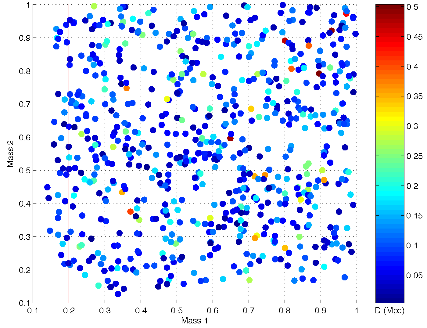
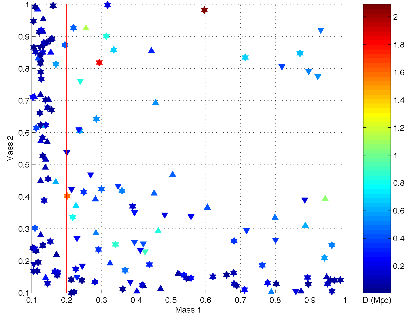
Figure 8: This figure shows the results of the Monte Carlo simulation used to measure the efficiency of the pipeline once parameter tuning had been completed; these detected triggers have survived all threshold and coincidence tests. The injections that are detected are shown as circles on the upper plot. The lower plot shows the injections that were not detected: stars correspond to missed injections in the triple coincident data, upward pointing triangles to the L1-H1 data and downward pointing triangles to the L1-H2 data. The $x$ and $y$ coordinates are the mass parameters $m_{1}$ and $m_{2}$ of each injection, respectively. The color of each injection represents the effective distance in the Hanford interferometers at which the waveform was injected (since the LHO interferometers limit the sensitivity of the search). The horizontal and vertical red lines show the edge of the template bank parameter space.

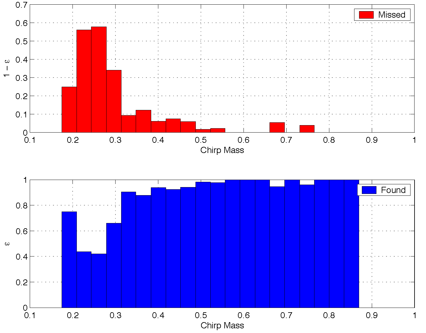
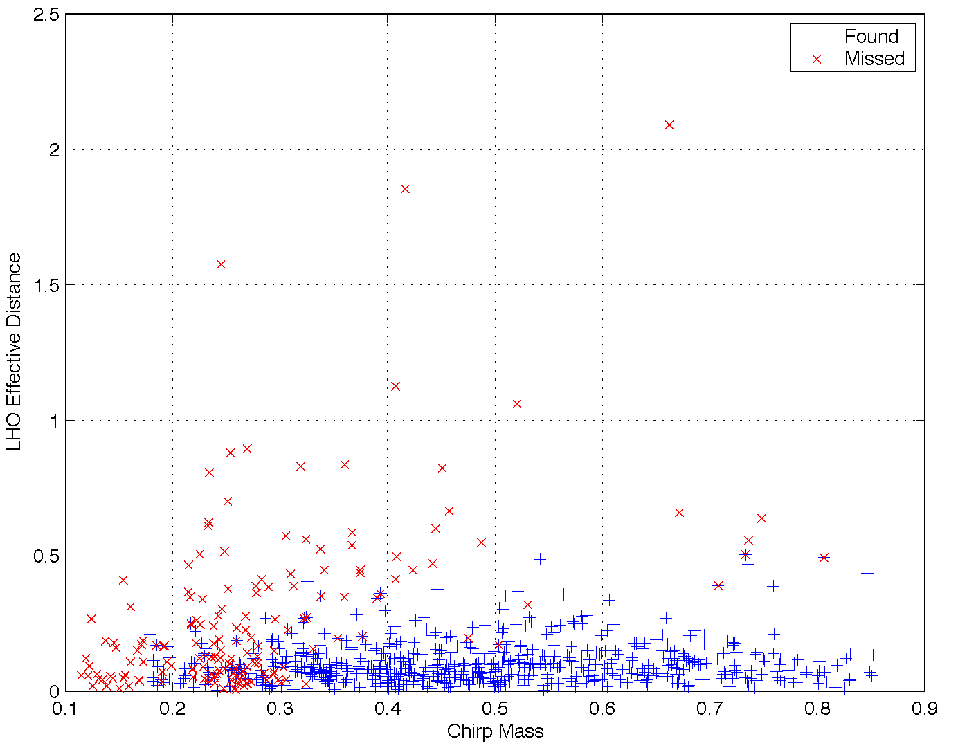
Figure 9: The upper two plots show the efficiency of the pipeline $\varepsilon$ and the loss of the search $1-\varepsilon$ as a function of the injected signal chirp mass $\mathcal{M}$ measured by the Monte Carlo Simulation. The lower plot shows the chirp mass and effective distance in LHO of the injections used to measure the pipeline efficiency; detected injections are shown with a $+$ and missed injections are shown with a $\times$. It can be seen that the efficiency of the pipeline is unity very close to unity for high values of $\mathcal{M}$ and falls as the chirp mass decreases. There appears to be an anomalously large value of $\varepsilon$ at $\mathcal{M}\approx 0.18$, however it can be seen from the lower plot that there were comparatively few injections at this chirp mass, so this may be an effect of small number statistics. Further Monte Carlo simulations will be able to test this hypothesis.

The angle $\psi$ is the third Euler angle that translates from the detectors frame to the radiation frame. The radiation frame is related to the frame of the binary by the angles $\iota$ and $\phi_{0}$, as shown in figure 8. Figure 9 shows the magnitude of the strain produced in an interferometer by binary with $\iota=\psi=0$ at various positions on the sky. It can be seen that the response of the detector is essentially omnidirectional, with the maximum sensitivity occurring when the source lies on the $z$-axis of the detector. Notice that there are four dead spots in the beam patters where the response of the interferometer is zero. These correspond to the locations where the binary is in the plane of the interferometer positioned half way between the $x$ and $y$-axes. We will often refer to an optimally oriented binary system. This is a binary located at sky position $\theta=0$ or $\pi/2$, (i.e. above or below the zenith of the detector) with an inclination angle of $\iota=0$. It is so called as this is the position in which the response of the detector to the binary is a maximum.

2.3.1 Higher Order Corrections to the Quadrupole Waveform

In the previous section we only considered the lowest order multipole radiation from a binary. The goal is to write down a waveform that is sufficiently accurate to use matched filtering to search for signals in detector noise. This requires accurate knowledge of the phase throughout the LIGO frequency band. In addition to higher order multipoles that contribute to the energy loss, there are relativistic corrections to the quadrupole formula and effects such as frame dragging and scattering of the gravitational wave by the gravitational field of the binary that change the phase evolution. Matched filtering is less sensitive to the amplitude evolution, however, so we may use the restricted post-Newtonian waveform as the matched filter template. The restricted post-Newtonian waveform models the amplitude evolution using the quadrupole formula, but includes higher-order $v/c$ corrections to the phase evolution. The formula for the orbital phase used in searches for binaries of component mass $\leq 3\,M_{\odot}$ is given by equation (7) of [Blanchet:1996pi]

$$\begin{split}\phi(t)&=\phi_{0}-\frac{1}{\eta}\left[\Theta^{\frac{5}{8}}+\left(\frac{3715}{8064}+\frac{55}{96}\eta\right)\Theta^{\frac{3}{8}}-\frac{3\pi}{4}\Theta^{\frac{1}{4}}\right.\\ &\quad+\left.\left(\frac{9\,275\,495}{14\,450\,688}+\frac{284\,875}{258\,048}\eta+\frac{1855}{2048}\eta^{2}\right)\Theta^{\frac{1}{8}}\right],\end{split}$$ (2.110)

where $\phi_{0}$ and $t_{c}$ are the orbital phase and time at which the binary coalescences and $\Theta$ is defined in equation (2.96).

2.3.2 The Stationary Phase Approximation

We will see in chapter 4 that we require the Fourier transforms, $\tilde{h}_{c}(f)$ and $\tilde{h}_{s}(f)$, of the inspiral waveforms rather than the time domain waveforms given above. In the search code, we could compute $\tilde{h}_{c}(f)$ using the Fourier transform of $h_{c}(t)$. This is computationally expensive, however, as it requires an additional Fourier Transform for each mass pair to be filtered. An alternative method is to use the stationary phase approximation[Mathews:1992] to express the chirp waveforms directly in the frequency domain[WillWiseman:1996, Cutler:1994]. Given a function

$$B(t)=A(t)\cos 2\phi(t)$$ (2.111)

where

$$\frac{d\ln A}{dt}\ll\frac{d\phi}{dt}$$ (2.112)

and

$$\frac{d^{2}\ln A}{dt^{2}}\ll\left(\frac{d\phi}{dt}\right)^{2}$$ (2.113)

then the stationary phase approximation to the Fourier transform of $B(t)$ is given by

$$\begin{split}\tilde{B}(f)&=\frac{1}{2}A(t)\left(\frac{df}{dt}\right)^{-\frac{1}{2}}\exp\left[-i\left(2\pi ft^{\prime}-2\phi(f)-\frac{\pi}{4}\right)\right]\\ &=\frac{1}{2}A(t)\left(\frac{df}{dt}\right)^{-\frac{1}{2}}\exp\left[-i\Psi(f)\right],\\ \end{split}$$ (2.114)

where $t^{\prime}$ is the time at which

$$\frac{d\phi(t)}{dt}=\pi f.$$ (2.115)

Now it is simple to calculate

$$\frac{df}{dt} =\frac{d}{dt}\left(\frac{\Omega}{\pi}\right)=\frac{d}{dt}\left(\frac{M^{\frac{1}{2}}}{\pi}a^{-\frac{3}{2}}\right)$$ (2.116)

$$=\frac{M^{\frac{1}{2}}}{\pi}\frac{dr}{dt}\left(-\frac{3}{2}a^{-\frac{5}{2}}\right)$$ (2.117)

$$=\frac{M^{\frac{1}{2}}}{\pi}\left(-\frac{64}{5}\frac{\mu M^{2}}{r^{3}}\right)\left(-\frac{3}{2}a^{-\frac{5}{2}}\right)$$ (2.118)

$$=\frac{96}{5}\frac{M^{\frac{5}{2}}\mu}{\pi}a^{-\frac{11}{2}}$$ (2.119)

$$=\frac{96}{5}\pi^{\frac{8}{3}}\mu M^{\frac{2}{3}}f^{\frac{11}{3}}$$ (2.120)

$$=\frac{96}{5}\pi^{\frac{8}{3}}\mathcal{M}^{\frac{5}{3}}f^{\frac{11}{3}}$$ (2.121)

where we have defined the chirp mass by

$$\mathcal{M}=\mu^{\frac{3}{5}}M^{\frac{2}{5}}.$$ (2.122)

To obtain the phase function $\Psi(f)$ we note that

$$f=\frac{1}{\pi}\frac{d\phi}{dt}$$ (2.123)

and we can invert the series in equation (2.110) to write $\Theta$ as a function of $f$. Substituting this result and the result for $df/dt$ into the equation for the stationary phase approximation, equation (2.114), we obtain the form of the inspiral chirps that we will use in matched filtering

$$\tilde{h}_{c}(f)=\frac{2GM_{\odot}}{c^{2}r}\left(\frac{5\mu}{96M_{\odot}}\right)^{\frac{1}{2}}\left(\frac{M}{\pi^{2}M_{\odot}}\right)^{\frac{1}{3}}f^{-\frac{7}{6}}\,\left(\frac{GM_{\odot}}{c^{3}}\right)^{-\frac{1}{6}}\,e^{i\Psi(f;M,\eta)}.$$ (2.124)

with the phase evolution given by

$$\begin{split}\Psi(f;M,\eta)&=2\pi ft_{c}-2\phi_{0}-\pi/4+\frac{3}{128\eta}\biggl{[}x^{-5}+\left(\frac{3715}{756}+\frac{55}{9}\eta\right)x^{-3}-16\pi x^{-2}\\ &\quad+\left(\frac{15\,293\,365}{508\,032}+\frac{27\,145}{504}\eta+\frac{3085}{72}\eta^{2}\right)x^{-1}\biggr{]},\end{split}$$ (2.125)

where $x=(\pi MfG/c^{3})^{1/3}$. Notice that in the definition of $\tilde{h}_{c}(f)$ we have absorbed the amplitude term $2GM_{\odot}/c^{2}r$ from $\tilde{h}_{+}$. This allows us to place $\tilde{h}_{c}$ at a cannonical distance of $r=1$ Mpc, as discussed later. Physically the chirp waveform should be terminate when the orbital inspiral turns into a headlong plunge, however the frequency at which this happens is not known for a pair of comparably massive objects. We therefore terminate the waveform at the gravitational wave frequency of a test particle in the innermost stable circular orbit of Schwarzschild (ISCO)[Wald:1984]

$$f_{\mathrm{isco}}=\frac{c^{3}}{6\sqrt{6}\pi GM},$$ (2.126)

which is a reasonable approximation of the termination frequency[Droz:1999qx]. Since the sine chirp is simply the orthogonal waveform to the cosine chirp, we have

$$\tilde{h}_{s}(f)=i\tilde{h}_{c}(f).$$ (2.127)

Together equations (2.124), (2.125) and (2.127) give the form of the chirps that we will use for the application of matched filtering discussed in chapter 4.

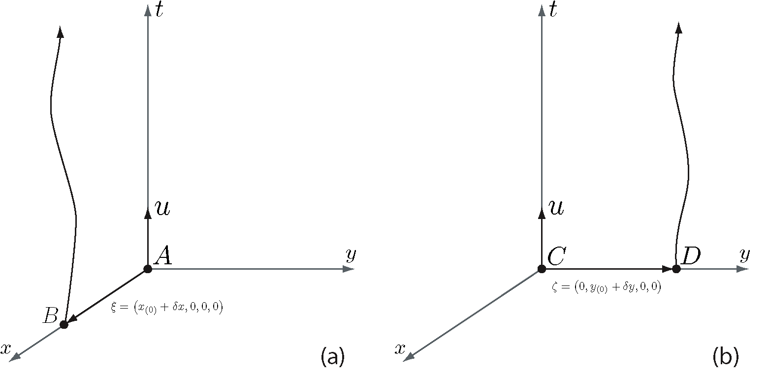
Figure 1: The axes shown in (a) and (b) represent Local Lorentz frames for particles $A$ and $C$ respectively. The effect of a gravitational wave in these frame can be described in terms of its effect on the vectors $\xi$ and $\zeta$ separating the particles at the origin from particles $B$ and $D$.

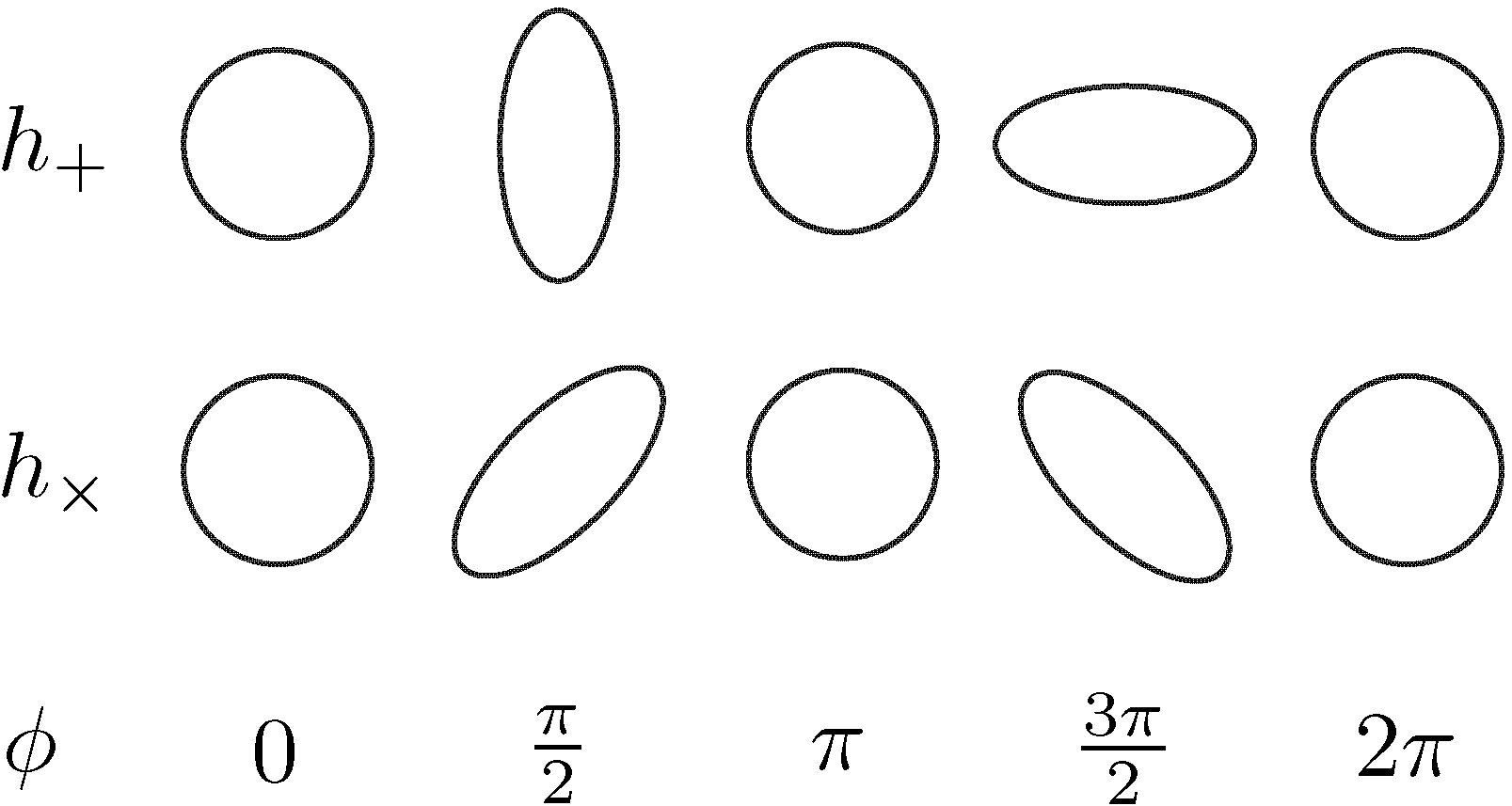
Figure 2: The effect of the two polarizations $h_{+}$ and $h_{\times}$ of a sinusoidal gravitational wave propagating through the page on a ring of test particles. As the phase $\phi$ of the gravitational wave changes through a complete cycle, the rings are distorted.

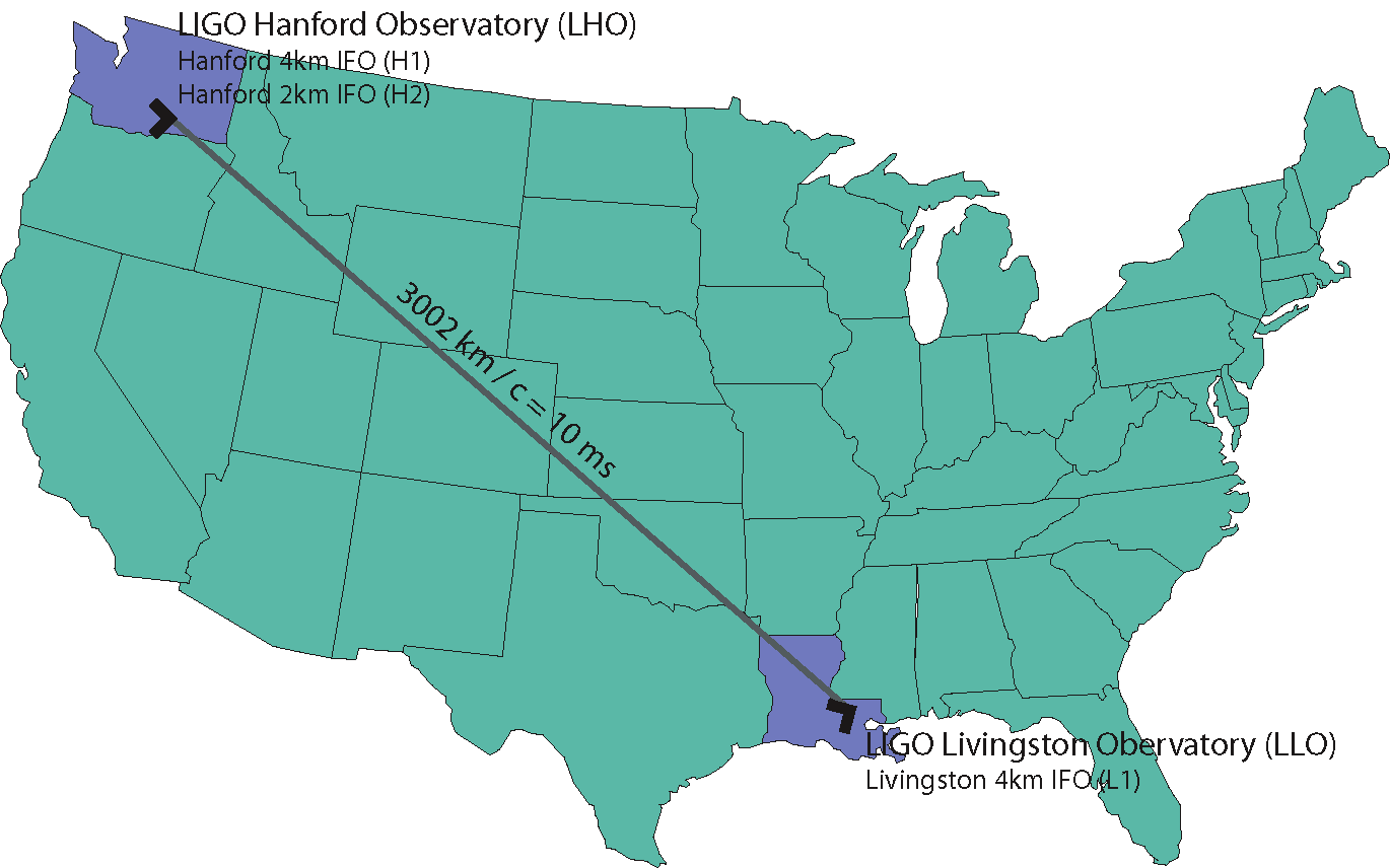
Figure 3: The location of the three LIGO interferometers. There are two interferometers at the LIGO Hanford Observatory (LHO) in Washington and one interferometer at the LIGO Livingston Observatory in Louisiana.

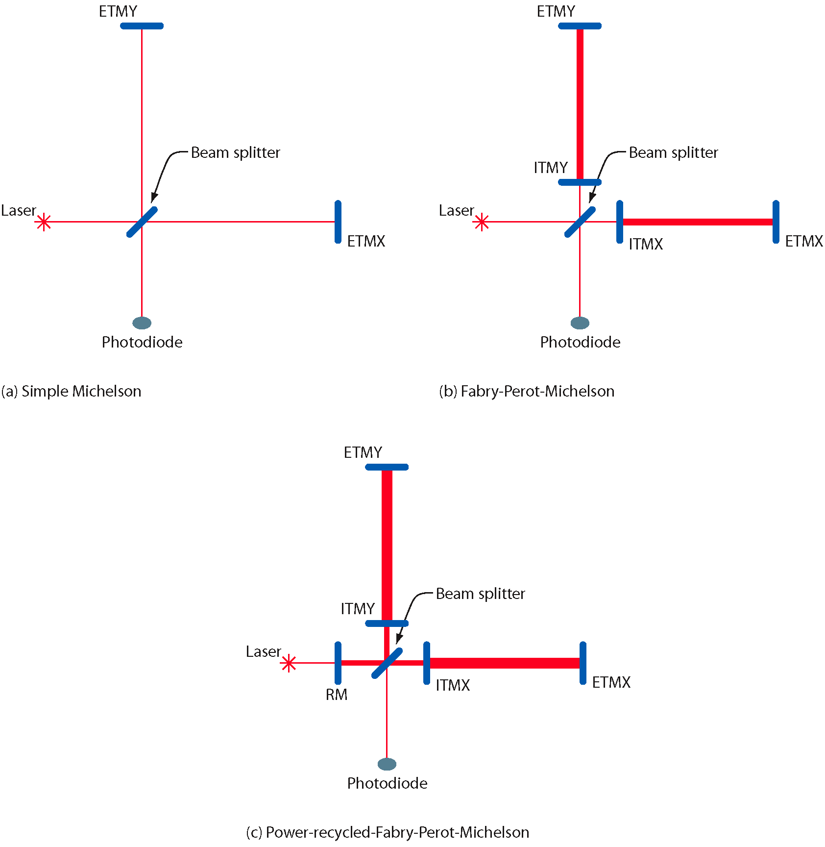
Figure 4: The possible optical configurations of first generation laser interferometers. The inner $x$ and $y$ test masses (mirrors) are denoted ITMX and ITMY respectively, and the end $x$ and $y$ test masses (mirrors) are denoted ETMX and ETMY respectively. The recycling mirror is denoted by RM. Initial LIGO is a power-recycled-Fabry-Perot interferometer, type (c) in this figure.

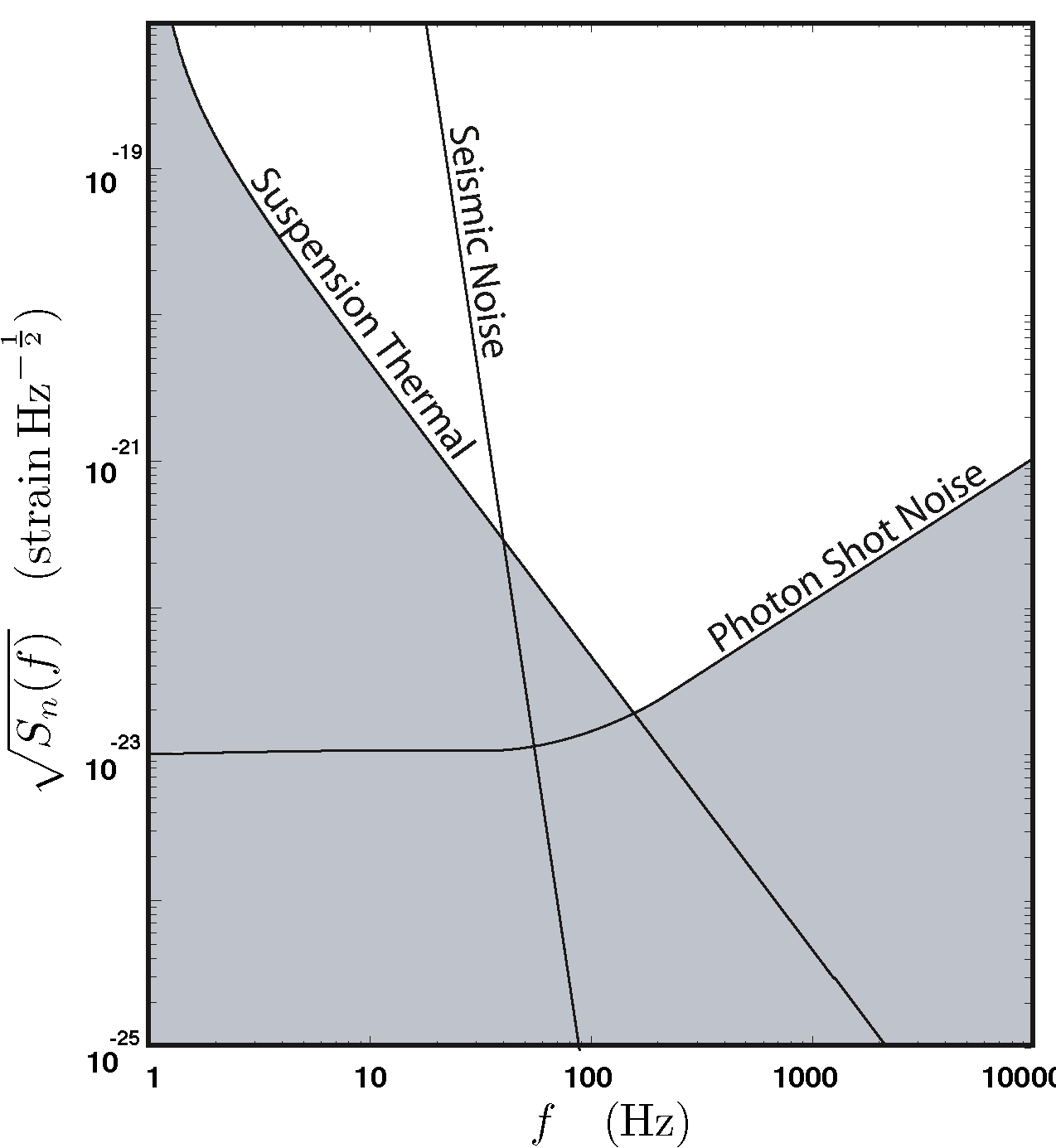
Figure 5: The fundamental noise sources of LIGO.

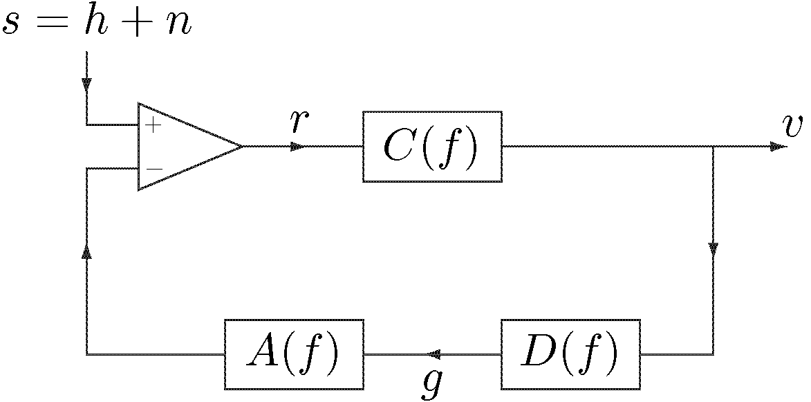
Figure 6: The differential more servo control loop. The figure shows the positions of three filters: the sensing function $C(f)$, the digital filter $D(f)$ and the actuation function $A(f)$. The input signal is $s$ and the measured signal is the error signal $v$. $r$ is the residual length of the cavity and $g$ is the control signal.

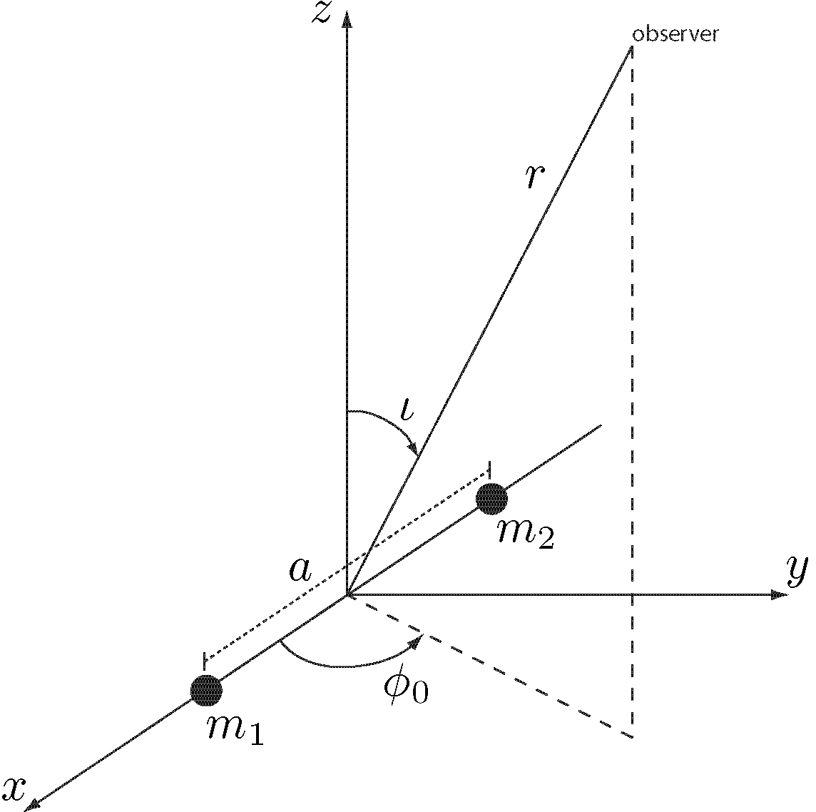
Figure 7: The parameters of a binary system with rotational axis aligned along the $z$-axis.

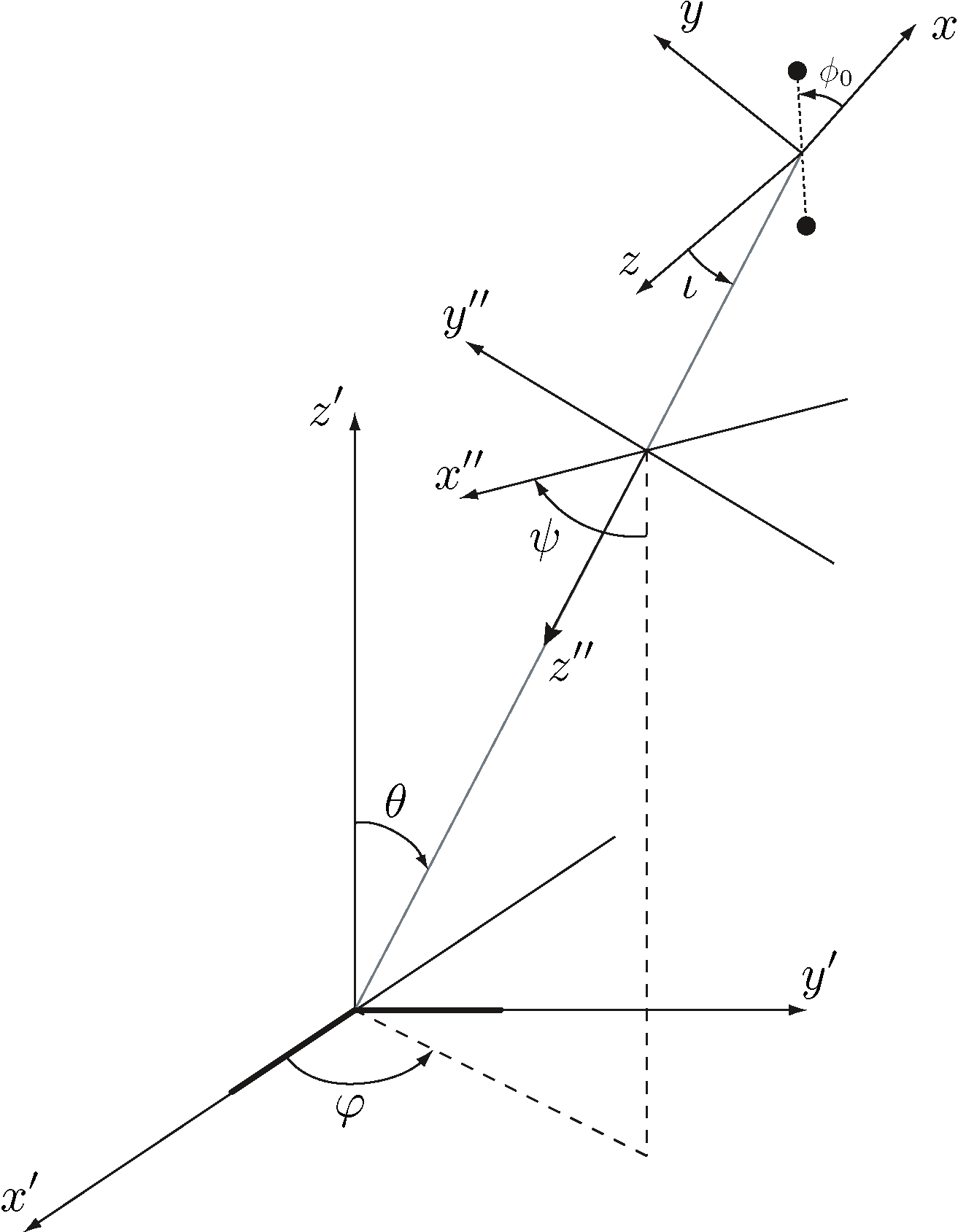
Figure 8: Euler angles of a binary system relative to the detector frame $x^{\prime},y^{\prime},z^{\prime}$. The frame of radiation basis is shown as $x^{\prime\prime}$ and $y^{\prime\prime}$.

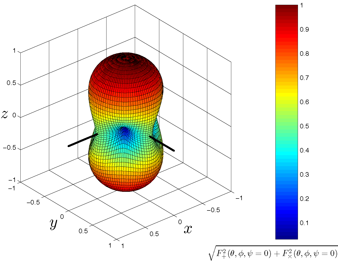
Figure 9: Level surface of the detector response function. The directions of the interferometer arms are shown.

Chapter 3 Binary Black Hole MACHOs

One of the most interesting current problems in astrophysics is that of dark matter. Dark matter is so called because it has eluded detection through its emission or absorption of electromagnetic radiation. Our knowledge of its existence comes from its gravitational interaction with luminous matter in the universe. There have been several ideas proposed to explain the nature of dark matter; chief among these are weakly interacting massive particles (WIMPs) and massive astrophysical compact halo objects (MACHOs)[Griest:1990vu]. WIMPs, supersymmetric particles produced as a relic of the big bang, are outside the scope of this thesis. No compelling reason exists to think that WIMPs will produce significant gravitational waves. In this chapter, we review the evidence for dark matter in the form of MACHOs in the Galactic halo. The nature of MACHOs is unknown; we review a proposal that suggests that if MACHOs are primordial black holes (PBHs) formed in the early universe, then some of the PBH MACHOs may be in binary systems[Nakamura:1997sm]. Searching for gravitational waves from the inspiral and coalescence of these binary black hole MACHOs (BBHMACHOs) is the motivation for this thesis.

3.1 Dark Matter In The Galactic Halo

Dark matter is detected by its gravitational interaction with luminous matter. Strong evidence for the presence of dark matter in the universe comes from the study of galactic rotation curves: measurements of the velocities of luminous matter in the disks of spiral galaxies as a function of galactic radius. Consider a simple rotational model for the disk of a spiral galaxy. Consider a star with mass $m_{s}$ orbiting at radius $r$ outside the disk of the galaxy. Newtonian dynamics tells us that if the mass inside radius $r$ is $m_{g}$ then

$$\frac{Gm_{g}m_{s}}{r^{2}}=\frac{m_{s}v_{s}^{2}}{r}$$ (3.1)

where $v_{s}$ is the velocity of the star and $G$ is the gravitational constant. Let us suppose that as we increase $r$, the change in the $m_{g}$ is negligible, which is a reasonable assumption towards the edge of the disk of a typical spiral galaxy. We can see from equation (3.1) that we would expect the velocity of stars at the edge of the galactic disk to fall off as

$$v_{s}\propto\frac{1}{\sqrt{r}},$$ (3.2)

when $r\gg R$, where $R$ is the radius containing most of the disk matter. Galactic rotation curves, determined using the Doppler shift of the $21$ cm hydrogen line, have been measured for several galaxies[Sancisi:1987]. It is found that the rotation curves do not fall off as expected. Instead the rotational velocities of galactic matter are measured to be constant out to the edge of the visible matter in the disk, as shown in figure 1. This surprising result suggests that 80%–90% of the matter in spiral galaxies is in the form of dark matter stretching out at least as far as the visible light.

A typical argument to understand the formation of galactic disks from baryonic matter considers an initially spherical distribution of baryonic matter rotating with some angular momentum, $L$. Over time the matter will lose energy through inelastic collisions. Since the angular momentum of the system is conserved, the initial distribution must collapse to a rotating disk. On the other hand, if the initially spherical distribution is composed of dark matter instead of baryons, the collisions will be elastic because the dark matter is weakly interacting. As a result of this, dark matter initially distributed in an isotropic sphere will maintain this distribution over time. Since we do not expect a spherical dark matter halo to collapse to a disk, the simplest possible assumption is that the dark halo is a spherical, isothermal distribution of dark matter. This suggests that dark matter will be distributed in an extended halo encompassing the luminous matter of a galaxy. If we assume that the density of the dark matter is $\rho(r)$ then the mass within a thin shell of a spherical halo is

$$dM(r)=4\pi r^{2}\rho(r)\,dr,$$ (3.3)

where $dr$ is the thickness of the shell. Using Newtonian dynamics, the velocity $v$ of a particle of mass $m$ at radius $r$ is

$$\begin{split}\frac{GM(r)m}{r^{2}}&=\frac{mv^{2}}{r}\\ v^{2}&=\frac{GM(r)}{r}.\end{split}$$ (3.4)

The galactic rotation curves tell us that the velocity is independent of the radius, so

$$M(r)=\frac{v^{2}r}{G}.$$ (3.5)

Differentiating this with respect to $r$ and substituting the result into equation (3.3), we obtain

$$\frac{dM(r)}{dr}=\frac{v^{2}}{G}=4\pi r^{2}\rho(r)$$ (3.6)

which gives

$$\rho(r)=\frac{v^{2}}{4\pi r^{2}G}.$$ (3.7)

If we assume that the dark and visible matter are in thermal equilibrium, we may use the measured rotational velocity of local stars about the galactic center as the velocity of the dark matter.

We can easily estimate the density of dark matter in the neighborhood of the Earth $\rho(r_{E})$ as follows. The earth is approximately $8$ kpc from the galactic center and the rotational velocity of objects at this radius is $v\sim 200$ $\mathrm{km\,s}^{-1}$. Using these values in equation (3.7), we find

$$\rho(r_{E})=7.6\times 10^{-25}\,\mathrm{g}\,\mathrm{cm}^{-3}.$$ (3.8)

More sophisticated modeling of the Galaxy[1995ApJ...449L.123G], suggests that the local halo density is

$$\rho(r_{E})=9.2_{-3.1}^{+3.8}\times 10^{-25}\,\mathrm{g}\,\mathrm{cm}^{-3}$$ (3.9)

or approximately $0.01\,M_{\odot}\,\mathrm{pc}^{-3}$.

Equation (3.7) applies only at intermediate radial distances. The data at small $r$ is consistent with the dark matter having a constant core density $\rho_{c}$ within a core radius $a$[Rix:1996]. The halo density then becomes

$$\rho(r)=\frac{\rho_{c}}{1+\left(\frac{r}{a}\right)^{2}}.$$ (3.10)

The values of $\rho_{c}$ and $a$ are obtained by fitting measured galactic rotation curves to equation (3.10) using data near the galactic center. There is, in fact, no evidence to suggest that halos are exactly spherical. In fact the halo density may be flattened[Rix:1996]. For a flattened halo a model of the dark matter density becomes

$$\rho(R,z)=\frac{\rho_{c}r^{2}_{c}}{a^{2}+R^{2}+z^{2}/q^{2}}$$ (3.11)

where $R$ and $z$ are galactocentric cylindrical coordinates and $q$ is a parameter that describes the flattening of the halo. At present there is no measurement of the extent of galactic halos beyond the luminous matter. For the Milky Way it is thought that the halo extends out to a radius of $\sim 50$kpc, although it is possible that it extends all the way out to the Andromeda galaxy at $\sim 700$ kpc.

3.2 MACHOs in the Galactic Halo

Galactic rotation curves provide strong evidence that spiral galaxies such as the Milky Way are surrounded by a large quantity of dark matter, but tell us nothing about the nature of this dark matter. A variety of candidates have been proposed to explain the nature of dark matter. These generally fall into two classes. The first class consists of elementary particles such as axions[Weinberg:1977ma] or weakly interacting massive particles (WIMPs)[Goodman:1984dc]. Such dark matter candidates are outside the scope of this thesis. Active searches for WIMPs and axions are underway and we refer to [Griest:1995gs] for a review of the particle physics dark matter candidates. The second class of dark matter candidates are known as massive astrophysical compact halo objects or MACHOs. MACHOs are objects such as brown dwarfs (stars with insufficient mass to burn hydrogen), red dwarfs (stars with just enough mass to induce nuclear fusion), white dwarfs (remnants of $1$–$8\,M_{\odot}$ stars) or black holes located in the halos of galaxies. Optical and infrared observations in the early 1990’s were not sensitive enough to constrain the fraction of the halo in MACHOs[1994MNRAS.266..775K] and the method of gravitational lensing was suggested as a method for detecting halo dark matter in the form of MACHOs[Paczynski:1985jf].

3.2.1 Gravitational Lensing of Light

Gravitational lensing is caused by the bending of light around a massive object. Assume that a MACHO produces a spherically symmetric gravitational field; the geometry of spacetime around the MACHO satisfies the Schwarzschild solution. Consider the scattering of light by a MACHO shown in figure 2, where $b$ the impact parameter of the light, the minimum distance of the photon to the MACHO. Recall that the lightlike orbits of Schwarzschild spacetime satisfy[Wald:1984]

$$\frac{d^{2}u}{d\phi^{2}}+u=\frac{3GM}{c^{2}b}u^{2}$$ (3.12)

where $u=b/r$ and $M$ is the mass of the MACHO. If $R$ is the size of the MACHO, then

$$\frac{3GMu^{2}}{c^{2}ub}=\frac{3GM}{c^{2}R}\frac{R}{b}\ll 1$$ (3.13)

if $b\gg R$. we can solve equation (3.12) perturbatively in the small parameter $\epsilon=R/b$ as follows. Write

$$u=u_{0}+\epsilon u_{1}+\cdots$$ (3.14)

and substitute into equation (3.12) to get

$$u_{0}^{\prime\prime}+\epsilon u_{1}^{\prime\prime}+\cdots+u_{0}+\epsilon u_{1}+\cdots=\frac{3GM}{c^{2}R}\left(u_{0}+\epsilon u_{1}+\cdots\right)^{2}$$ (3.15)

where prime denotes differentiation with respect to $\phi$. At leading order,

$$u_{0}^{\prime\prime}+u_{0}=0$$ (3.16)

has solution

$$u_{0}=A\sin\left(\phi+\phi_{0}\right)$$ (3.17)

where $A$ and $\phi_{0}$ are constants. We are free to choose any value for $\phi_{0}$ as it simply chooses an orientation for the axes in figure 2, so let $\phi_{0}=0$. Since $\phi=\pi/2$ gives the distance of closed approach, we find $A=b/r_{\mathrm{min}}=1$. Now $u_{1}$ satisfies

$$\begin{split}u_{1}^{\prime\prime}+u_{1}&=\frac{3GM}{c^{2}R}\sin^{2}\phi\\ &=\frac{3GM}{2c^{2}R}\left(1-\cos 2\phi\right).\end{split}$$ (3.18)

Inspection suggests a solution of the form

$$u_{1}=\frac{3GM}{2c^{2}R}+\alpha\cos 2\phi.$$ (3.19)

Substituting this into equation (3.18) we find that

$$-4\alpha\cos 2\phi+\frac{3GM}{2c^{2}R}+\alpha\cos 2\phi=\frac{3GM}{2c^{2}R}-\frac{3GM}{2c^{2}R}\cos 2\phi$$ (3.20)

and so $\alpha=GM/2c^{2}R$. The solution for $u$, up to first order, is therefore

$$u=\sin\phi+\frac{GM\epsilon}{2c^{2}R}\left(3+\cos 2\phi\right).$$ (3.21)

As $r\rightarrow\infty$, $u\rightarrow 0$ and $\phi\rightarrow-\delta/2$, so

$$0=\sin\left(-\frac{\delta}{2}\right)+\frac{GM}{2c^{2}b}\left(3+\cos(-\delta)\right)$$ (3.22)

For small $\delta$, $\sin(-\delta/2)\approx-\delta/2$ and $\cos(-\delta)\approx 1$, so

$$0 \approx-\frac{\delta}{2}+\frac{2GM}{c^{2}b}$$ (3.23)

$$\delta \approx\frac{4GM}{c^{2}b}$$ (3.24)

The total deflection of the light is therefore

$$\delta=\frac{4GM}{c^{2}b}.$$ (3.25)

Suppose a MACHO lens is at a distance $D_{\mathrm{SL}}$ from a source star and an observer is at a distance $D_{\mathrm{L}}$ from the MACHO as shown in figure 3. Then the ray of light from the source that encounters the MACHO with critical impact parameter $r_{\mathrm{E}}$ will reach the observer. Simple geometry, using the small angle approximations, shows that

$$\delta=\theta_{\mathrm{S}}+\theta_{\mathrm{O}}=\frac{r_{\mathrm{E}}}{D_{\mathrm{L}}}+\frac{r_{\mathrm{E}}}{D_{\mathrm{SL}}}=\frac{4GM}{c^{2}r_{\mathrm{E}}}$$ (3.26)

therefore the observer sees the lens light when the ray is at the Einstein radius, $r_{\mathrm{E}}$, given by

$$r_{\mathrm{E}}=\sqrt{\frac{4GM}{c^{2}}\frac{D_{\mathrm{SL}}D_{\mathrm{L}}}{D_{\mathrm{SL}}+D_{\mathrm{L}}}}.$$ (3.27)

If the source, MACHO and observer are collinear, as shown in figure 3 the observer sees a bright ring of radius $r_{\mathrm{E}}$ around the MACHO. The angular radius of this ring is the Einstein angle,

$$\theta_{\mathrm{E}}=\sqrt{\frac{4GM}{c^{2}}\frac{D_{\mathrm{SL}}}{D_{\mathrm{L}}\left(D_{\mathrm{SL}}+D_{\mathrm{L}}\right)}}.$$ (3.28)

In the realistic case of slight misalignment, then the lensed star will appear as two small arcs. Consider a MACHO of mass $0.5\,M_{\odot}$ at a distance of $D=25$ kpc lensing a star in the Large Magellanic Cloud (LMC) at a distance of $50$ kpc. Then

$$\theta_{\mathrm{E}}=\sqrt{\frac{2GM}{Dc^{2}}}\approx 10^{-10}\approx 2"\times 10^{-5},$$ (3.29)

too small to be resolved by optical telescopes. Fortunately the lensing produces an apparent amplification of the source star by a factor [1964MNRAS.128..295R]

$$A=\frac{v^{2}+2}{v\sqrt{v^{2}+4}},$$ (3.30)

where $v=\beta/\theta_{\mathrm{E}}$, and $\beta$ is the angle between the observer-lens and observer-star lines. Since objects in the halo are in motion,

$$\beta(t)=\sqrt{(v_{\perp}t)^{2}+\beta_{\mathrm{min}}^{2}},$$ (3.31)

where $v_{\perp}$ is the transverse velocity of the lens relative to the line of sight, $\beta_{\mathrm{min}}$ is the closest approach of the lens to the source, and $t$ is the time to the point of closest approach[Paczynski:1985jf, Griest:1990vu]. Searches for the amplification of stars caused by gravitational lensing of $\theta_{\mathrm{E}}\sim$ micro arc seconds are referred to as gravitational microlensing surveys. Such surveys measure magnification of the star and the duration of the microlensing event. Unfortunately it is not possible to determine the size of the the lens from these measurements.

3.2.2 Gravitational Microlensing Surveys

Several research groups are engaged in the search for microlensing events from dark matter[Alcock:2000ph, Afonso:2002xq]. By monitoring a large population of well resolved background stars such as the LMC, constraints can be placed on the MACHO content of the halo. The MACHO project has conducted a 5.7 year survey monitoring 11.9 million stars in the LMC to search for microlensing events[Alcock:2000ph] using an automated search algorithm to monitor the light curves of LMC stars. Optimal filtering is used to search for light curves with the characteristic shape given by equation (3.30).

Since the effect of microlensing is achromatic, light curves are monitored in two different frequency bands to reduce the potential background sources which may falsely contribute to the microlensing rate. Background events include variable stars in the LMC (known as bumpers[1996astro.ph..6165A]), which can usually be rejected as the fit of the light curves to true microlensing curves is poor. Supernovae occurring behind the LMC are the most difficult to cut from the analysis. The MACHO project reported 28 candidate microlensing events in the 5.7 year survey of which 10 were thought to be supernovae behind the LMC and 2–4 were expected from lensing by known stellar populations. They report an excess of 13–17 microlensing events, depending on the selection criteria used.

The optical depth, $\tau$, is the probability that a given source star is amplified by a factor $A>1.34$[Paczynski:1985jf]. This is just the probability that the source lies on the sky within a disk of radius $\theta_{\mathrm{E}}$ around a microlensing object and is given by[Alcock:1995zx]

$$\tau=\frac{4\pi G}{c^{2}}\int_{0}^{L}\rho(l)\frac{l(L-l)}{L}\,dl,$$ (3.32)

where $L=D_{\mathrm{SL}}+D_{\mathrm{L}}$ is the observer-star distance and $l=D_{\mathrm{L}}$ is the observer-lens distance. For the spherical halo given in equation (3.10) with density

$$\rho(r)=0.0079\frac{R_{0}^{2}+a^{2}}{r^{2}+a^{2}}\,M_{\odot}\,\mathrm{pc}^{-3},$$ (3.33)

where $R_{0}=8.5$ kpc is the Galactocentric radius of the Sun and a galactic core radius of $a=5$ kpc, the predicted optical depth towards the LMC (assumed to be at $50$ kpc) is[Alcock:1995zx]

$$\tau_{\mathrm{LMC}}=4.7\times 10^{-7}.$$ (3.34)

The optical depth towards the LMC measured by the MACHO project microlensing surveys is

$$\tau_{\mathrm{LMC}}=1.2_{-0.3}^{+0.4}\times 10^{-7}.$$ (3.35)

This suggests that the fraction of the halo in MACHOs is less that $100\%$, but does not exclude a MACHO halo.

The number of observed MACHO events and the time scales of the light curves can be compared with various halo models. The MACHO project has performed a maximum-likelihood analysis in which the halo MACHO fraction $f$ and MACHO mass $m$ are free parameters. For the standard spherical halo, they find the most likely values are $f=20\%$ and $m=0.45\,M_{\odot}$. The $95\%$ confidence interval of on the MACHO halo faction is $f=8\%$–$50\%$ and the $95\%$ confidence interval of on the MACHO mass is $0.15$–$0.9\,M_{\odot}$. The total mass in MACHOs out to $50$ kpc is found to be $9_{-3}^{+4}\times 10^{10}\,M_{\odot}$, independent of the halo model[Alcock:2000ph]. The EROS collaboration has recently published results of a search for microlensing events towards the Small Magellanic Cloud (SMC)[Afonso:2002xq]. The EROS result further constrains the MACHO fraction of a standard halo in the mass range of interest to less than $25\%$; they do not exclude a MACHO component of the halo, however.

3.3 Gravitational Waves from Binary Black Hole MACHOs

Since the microlensing surveys have shown that $\sim 20\%$ of the halo dark matter may be in the form of $\sim 0.5\,M_{\odot}$ MACHOs, it is natural to ask what the MACHOs may be. As we mentioned above, it has been proposed that MACHOs could be baryonic matter in the form of brown dwarfs, objects lighter than $\sim 0.1\,M_{\odot}$ that do not have sufficient mass to sustain fusion, however, this is inconsistent with the observed masses of MACHOs. The fraction of the halo in red dwarfs, the faintest hydrogen burning stars with masses greater than $\sim 0.1\,M_{\odot}$, can be constrained using the Hubble Space Telescope. Hubble observations may also be used to constrain the fraction of the halo in brown dwarfs. The results indicate that brown dwarfs make up less than $\sim 3\%$ and red dwarfs less than $\sim 1\%$ of the halo[Graff:1995ru, Graff:1996rz]. A third possible candidate for baryonic MACHOs is a population of ancient white dwarfs in the halo. White dwarfs are the remnants of stars of mass $1$–$8\,M_{\odot}$ and have masses of $\sim 0.6\,M_{\odot}$. Although they seem to be natural candidates for MACHOs, proper motion searches for halo white dwarfs have been conducted and no candidates have been found[2002A&A...389L..69G, 2002ApJ...573..644N, Creze:2004gs]. Creeze et al. combined the results of previous surveys to find that $4\%$ ($95\%$ confidence level) of the halo is in the form of white dwarfs[Creze:2004gs].

It is possible that there is an over dense clump of MACHOs in the direction of the LMC[1996ApJ...473L..99N], the lenses are located in the LMC itself[Salati:1999gd] or the lenses are in the disk of the galaxy[Evans:1997hq]. If the MACHOs detected by microlensing are truly in the halo, however, it is possible that MACHOs are non-baryonic matter such as black holes [Finn:1996dd, Nakamura:1997sm]. Black holes of mass $\sim 0.5\,M_{\odot}$ could not have formed as a product of stellar evolution and so they must have been formed in the early universe[1967SvA....10..602Z, 1974MNRAS.168..399C]. Several mechanisms have been proposed to form primordial black holes with the masses consistent with the MACHO observations. These include multiple scalar fields during inflation[Yokoyama:1995ex], chaotic inflation[Yokoyama:1999xi] or reduction of the speed of sound during the QCD phase transition[Jedamzik:1996mr]. We do not consider these formation mechanisms in detail here; it is sufficient for our purposes that PBHs with masses consistent with microlensing observations can form. If the MACHOs are primordial black holes then there must be a large number of them in the halo. The total mass in MACHOs out to $50$ kpc is $9\times 10^{10}\,M_{\odot}$, as measured by microlensing surveys. If these are $0.5\,M_{\odot}$ PBHs then there will be at least $\sim 1.8\times 10^{11}$ PBHs in the halo. With such a large number of PBHs in the halo it is natural to assume that some of these may be in binary systems.

Nakamura et al.[Nakamura:1997sm] considered PBHs formed when the scale factor of the universe $R$, normalized to unity at the time of matter-radiation equality, is

$$R_{f}=\sqrt{GM_{\mathrm{BH}}}{c^{2}L_{\mathrm{eq}}}=1.2\times 10^{-8}\left(\frac{M_{\mathrm{BH}}}{M_{\odot}}\right)^{\frac{1}{2}}(\Omega h^{2}),$$ (3.36)

where $L_{\mathrm{eq}}$ is the Hubble horizon scale at the time of matter-radiation equality, $\Omega$ is the fraction of the closure density in PBHs and $h$ is the Hubble parameter in units of $100$ km s^-1. The age and temperature of the universe at this epoch are $\sim 10^{-5}$ seconds and $\sim 1$ GeV, respectively. By considering a pair of black holes that have decoupled from the expansion of the universe to form a bound system interacting with a third black hole, which gives the pair angular momentum to form a binary, they showed that the distribution of the semi-major axis, $a$, and eccentricity, $e$ of a population of binary black hole MACHOs is

$$f(a,e)\,da\,de=\frac{3ea^{\frac{1}{2}}}{2\bar{x}^{\frac{3}{2}}(1-e^{2})^{\frac{3}{2}}}\,da\,de$$ (3.37)

where $\bar{x}$ is the mean separation of the black hole MACHOs at the time of matter-radiation equality, given by

$$\bar{x}=1.1\times 10^{16}\left(\frac{M}{M_{\odot}}\right)^{\frac{1}{3}}\left(\Omega h^{2}\right)^{-\frac{4}{3}}\,\mathrm{cm},$$ (3.38)

The coalescence time of a binary by the emission of gravitational waves is approximately given by [Peters:1964]

$$t=t_{0}\left(\frac{a}{a_{0}}\right)^{4}\left(1-e^{2}\right)^{\frac{7}{2}},$$ (3.39)

where $t_{0}=10^{10}$ years and

$$a_{0}=2\times 10^{11}\left(\frac{M}{M_{\odot}}\right)^{\frac{3}{4}}\,\mathrm{cm}$$ (3.40)

is the semimajor axis of a binary with circular orbit which coalesces in time $t_{0}$. Integrating equation (3.37) for fixed $t$ using equation (3.39), Nakamura et al.[Nakamura:1997sm] found the probability distribution $f_{t}(t)$ for the coalescence time is

$$f_{t}(t)\,dt=\frac{3}{29}\left[\left(\frac{t}{t_{\mathrm{max}}}\right)^{\frac{3}{37}}-\left(\frac{t}{t_{\mathrm{max}}}\right)^{\frac{3}{8}}\right]\frac{dt}{t},$$ (3.41)

where $t_{\mathrm{max}}=t_{0}(\bar{x}/a_{0})^{4}$. The number of coalescing binaries with $t\sim t_{0}$ is then $\sim 5\times 10^{8}$ for $\Omega h^{2}=0.1$, so the event rate of coalescing binaries is $\sim 5\times 10^{-2}$ events per year per galaxy. Ioka et al.[Ioka:1998nz] performed more detailed studies of binary black hole MACHO formation in the early universe and found that, within a $50\%$ error, the distribution function and the rate of coalescence given in [Nakamura:1997sm] agree with numerical simulations. The event rate of coalescing binary black hole MACHOs is therefore

$$R_{\mathrm{BBHMACHO}}=5\times 10^{-2}\times 2^{\pm 1}\,\mathrm{yr}^{-1}\,\mathrm{galaxy}^{-1}.$$ (3.42)

This rate is significantly higher than the coalescence rate of binary neutron stars, which is[Kalogera:2004tn]

$$R_{\mathrm{BNS}}=8.3\times 10^{-5}\times 2^{\pm 1}\,\mathrm{yr}^{-1}\,\mathrm{galaxy}^{-1}.$$ (3.43)

It must be emphasized that several neutron star binaries have been observed, but there are no observations of black hole MACHO binaries.

The distance to which we can detect a binary inspiral is usually expressed in terms of the characteristic strain, $h_{\mathrm{char}}$ of the binary. This represents the intrinsic amplitude of the signal at some frequency times the square-root of the number of cycles over which the signal is observed at that frequency

$$h_{\mathrm{char}}(f)=|f\tilde{h}(f)|\approx h\sqrt{n}$$ (3.44)

For an inspiral signal this is given by[Thorne:1982cv]

$$h_{\mathrm{char}}(f)=4\times 10^{-21}\left(\frac{\mathcal{M}}{{M_{\odot}}}\right)^{\frac{5}{6}}\left(\frac{f}{100\,\mathrm{Hz}}\right)^{-\frac{1}{6}}\left(\frac{r}{20\,\mathrm{Mpc}}\right)^{-1},$$ (3.45)

where $r$ is the distance to the binary and $\mathcal{M}$ is the chirp mass. For comparison with signal strength, the detector sensitivity is better expressed in terms of the root mean square (RMS) dimensionless strain per logarithmic frequency interval

$$h_{\mathrm{rms}}=\sqrt{fS_{n}(f)},$$ (3.46)

where $s$ is the detector strain output in the absence of a gravitational wave signal and $S_{n}(f)$ is the power spectral density of $s$. If the value of $h_{\mathrm{char}}>\left(\textrm{a few}\right)\times h_{\mathrm{rms}}$, then the binary will be detectable. Figure 4 shows the characteristic strain of a binary consisting of two $0.5\,M_{\odot}$ black holes at $10$ Mpc compared to the RMS noise for initial LIGO. It can be seen that the inspiral signal lies significantly above the noise, so these MACHO binaries could be excellent source for initial LIGO. Nakamura et al.[Nakamura:1997sm] showed that the rate of MACHO binaries could be as high as $3$ yr^-1 at a distance of $15$ Mpc, under their model assumptions.

3.4 Binary Black Hole MACHO Population Model

The goal of this thesis is to search for gravitational waves from binary black hole MACHOs described in the previous section. In the absence of a detection, however, we wish to place an upper limit on the rate of binary black hole MACHO inspirals in the galaxy. We can then compare the predicted rate with that determined by experiment. We will see later that in order to determine an upper limit on the rate, we need to measure the efficiency $\varepsilon$ of our search to binary black hole MACHOs in the galactic halo. We do this using a Monte Carlo simulation which generates a population of binary black hole MACHOs according to a given probability density function (PDF) of the binary black hole MACHO parameters. Using the set of parameters generated by sampling the PDF, we can simulate the corresponding inspiral waveforms on a computer. We then digitally add the simulated waveforms to the output of the gravitational wave detector. By analyzing the interferometer data containing the simulated signals, we can determine how many events from the known source distribution we find. The efficiency of the search is then simply

$$\varepsilon=\frac{\textrm{number of signals found}}{\textrm{number of signals injected}}.$$ (3.47)

Recall that an inspiral waveform is described by the following nine parameters:

$$\begin{split}t_{c}&\quad\textrm{the end time of the inspiral},\\ m_{1}&\quad\textrm{the mass of the first binary component},\\ m_{2}&\quad\textrm{the mass of the second binary component},\\ \iota&\quad\textrm{the inclination angle of the binary},\\ \phi_{0}&\quad\textrm{the oribital phase of the binary},\\ \psi&\quad\textrm{the polarization angle of the binary},\\ (\theta,\varphi)&\quad\textrm{the sky coordinates of the binary},\\ r&\quad\textrm{the distance to the binary}.\end{split}$$

To simulate a population of BBHMACHOs in the halo we need to generate a list of these parameters that correctly samples their distributions.

We first address the generation of inspiral end time, $t_{c}$. The nature of the noise in the interferometers changes with time, as does the orientation of the detectors with respect to the galaxy as the earth rotates about its axis over a sidereal day. To sample the changing nature of the detector output, the Monte Carlo population that we generate contains many inspiral signals with end times distributed over the course of the science run. We generate values of $t_{c}$ at fixed intervals starting from a specified time $t_{0}$. The fixed interval is chosen to be $2048+\pi\approx 2051.141592653$ sec. This allows us to inject a significant number of signals over the course of the two month run with the signals far enough apart that they do not dominate the detector output. The interval is chosen to be non-integer to avoid any possible periodic behavior associated with data segmentation. The start time for the Monte Carlo, $t_{0}$, is chosen from a uniform random distribution in the range $t_{\mathrm{start}}-2630/\pi\leq t_{0}\leq t_{\mathrm{start}}$, where $t_{\mathrm{start}}$ is the time at which the science run begins. We stop generating inspiral parameters when $t_{c}>t_{\mathrm{end}}$ the time at which the second science run ends. For each generated end time, $t_{c}$ we generate the other inspiral waveform parameters.

We obtain the distribution of the mass parameters $(m_{1},m_{2})$ from the microlensing observations of MACHOs in the galactic halo, described in section 3.2.1, which suggest that the most likely MACHO mass is between $0.15$ and $0.9\,M_{\odot}$. In the absence of further information on the mass distribution we simply draw each component mass from a uniform distribution in this range. We increase the range slightly to better measure the performance of our search at the edge of the parameter space. We also note that the search for binary neutron stars covers the mass range $1$ to $3\,M_{\odot}$, so we continue the BBHMACHO search up to $1\,M_{\odot}$ rather than terminating it at $0.9\,M_{\odot}$. We therefore generate each BBHMACHO mass parameter, $m_{1}$ or $m_{2}$, from a uniform distribution of masses between $0.1$ and $1.0\,M_{\odot}$.

The angles $\iota$ and $\phi_{0}$ are generated randomly to reflect a uniform distribution in solid angle; $\cos\iota$ is uniform between $-1$ and $1$ and $\phi_{0}$ is uniform between $0$ and $2\pi$. The polarization angle $\psi$ is also generated from a uniform distribution between $0$ and $2\pi$.

To generate the spatial distribution of BBHMACHOs, we assume that the distribution in galactocentric cylindrical coordinates, $(R,\theta,z)$, follows the halo density given by equation (3.11), that is,

$$\rho(r)\propto\frac{1}{a^{2}+R^{2}+z^{2}/q^{2}}$$ (3.48)

where $a$ is the halo core radius and $q$ is the halo flattening parameter. We can see that this distribution is independent of the angle $\theta$, so we generate $\theta$ from a uniform distribution between $0$ and $2\pi$. If we make the coordinate change $z/q\rightarrow z$, we may obtain a probability density function (PDF) for the spatial distribution of the MACHOs given by

$$f(R,z)\,R\,dR\,dz\propto\frac{1}{a^{2}+R^{2}+z^{2}}\,R\,dR\,dz.$$ (3.49)

We wish to randomly sample this PDF to obtain the spatial distribution of the BBHMACHOs. Once we have obtained a value of the new coordinate $z$, we simply scale by $q$ to obtain the original value of $z$. Recall that for a probability density function $f(x)$ the cumulative distribution $F(X)$ given by

$$F(X)=\int_{-\infty}^{X}f(x)\,dx$$ (3.50)

with $F(X)\in[0,1]$ for all $f(x)$. If we generate a value of $u$ from a uniform distribution between $[0,1]$ and solve

$$\int_{-\infty}^{x}f(x^{\prime})\,dx^{\prime}=u$$ (3.51)

for $x$ then we will uniformly sample the probability distribution given by $f(x)$. Notice, however, that PDF in equation (3.49) is a function of the two random variables $R$ and $z$, rather than a single variable $x$ as in equation (3.51). Let us make the coordinate change

$$\begin{split}R&=r\cos\varphi,\\ z&=r\sin\varphi\\ \end{split}$$ (3.52)

and so

$$\begin{split}\tan\varphi&=\frac{z}{R},\\ r^{2}&=R^{2}+z^{2}.\\ \end{split}$$ (3.53)

Equation (3.49) becomes

$$\begin{split}\mathcal{K}\int\int\frac{1}{a^{2}+R^{2}+z^{2}}\,R\,dR\,dz&=\mathcal{K}\int\int\frac{r\cos\varphi}{a^{2}+r^{2}}\,r\,dr\,d\varphi\\ &=\mathcal{K}\int_{-1}^{1}d\sin\varphi\int_{0}^{r_{\mathrm{max}}}\frac{r^{2}}{a^{2}+r^{2}}\,dr\\ &=\mathcal{K}\left[\sin\varphi\right]_{-1}^{1}\left[r-a\arctan\left(\frac{r}{a}\right)\right]_{0}^{r_{\mathrm{max}}},\end{split}$$ (3.54)

where $r_{\mathrm{max}}=50$ kpc is the extent of the halo and $\mathcal{K}$ is a constant that normalizes the PDF to unity. We can see immediately from equation (3.54) that $\sin\varphi$ is uniformly distributed between $-1$ and $1$. Now consider the PDF for $r$ given by

$$f(r)=\mathcal{K}\left[r-a\arctan\left(\frac{r}{a}\right)\right]_{0}^{r_{\mathrm{max}}}$$ (3.55)

with normalization constant

$$\mathcal{K}=\left[R_{\mathrm{max}}-a\arctan\left(\frac{R_{\mathrm{max}}}{a}\right)\right]^{-1}$$ (3.56)

To sample the distribution for $r$, generate a random variable $u$ uniform between $0$ and $1$ and find the root of

$$r-a\arctan\left(\frac{r}{a}\right)-u\left[R_{\mathrm{max}}-a\arctan\left(\frac{R_{\mathrm{max}}}{a}\right)\right]=0.$$ (3.57)

We can see that the value of $r$ that solves equation (3.57) must lie between $0$ and $R_{\mathrm{max}}$ and that the left hand side is a monotonically increasing function of $r$. We may therefore use a simple bisection to solve for the value of $r$. The values of $r$ and $\varphi$ are easily inverted for $R$ and $z$ using equation (LABEL:eq:probcoordtrans).

This method was implemented in lalapps_minj and figure 5 shows a histogram of the first mass parameter generated the by the Monte Carlo code. It can be seen that this is uniform between $0.1$ and $1.0\,M_{\odot}$, as expected. Figure 6 shows the spatial distribution of BBHMACHO binaries for a spherical, $q=1$, halo that extends to $R_{\mathrm{max}}=50\,\mathrm{kpc}$ with a core radius of $a=5$ kpc. Since the software that simulates inspiral waveforms expects the position of the inspiral to be specified in equatorial coordinates, the population Monte Carlo code also generates the coordinates of the inspiral as longitude, latitude and distance from the center of the earth, as shown in figure 7. We will return to the use of population Monte Carlos in chapter 7.

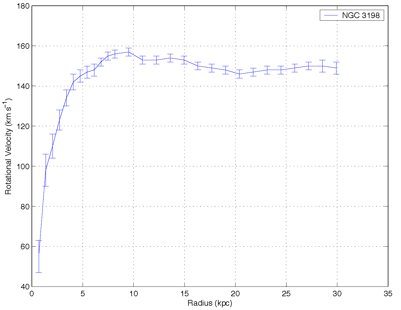
Figure 1: The results of observations of the hydrogen $21$ cm line of the spiral galaxy NGC 3198 show that the rotation curve is flat out to the last measured point at $30$ kpc[1989A&A...223...47B]. This implies a large discrepancy between the observed rotation curve and that predicted from light observations.

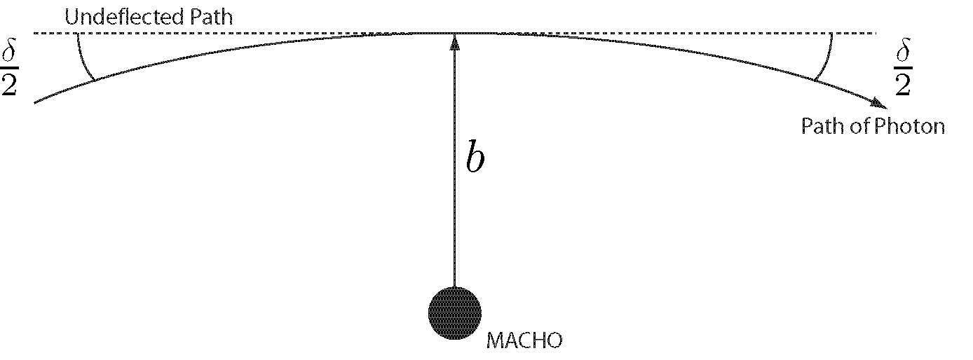
Figure 2: A photon will be scattered by the curvature of spacetime caused to the gravitational field of a MACHO. If the closest approach of the photon is $b$, it will be deflected by an angle $\delta=4GM/c^{2}b$.

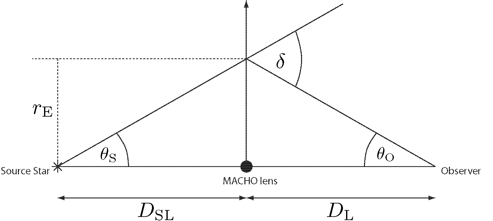
Figure 3: The geometry of microlensing of light from a source star by a MACHO showing the definition of the Einstein radius, $r_{\mathrm{E}}$.

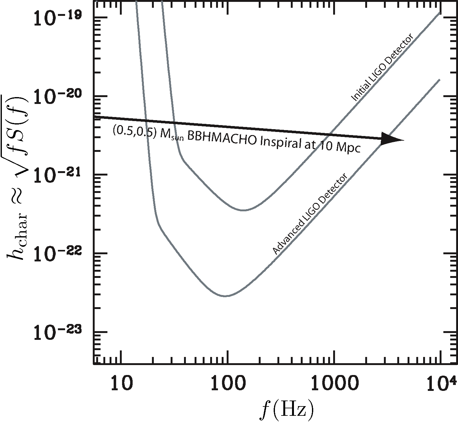
Figure 4: The sensitivity of LIGO to a binary black hole MACHO inspiral can be considered in terms of comparison between the characteristic strain $h_{\mathrm{char}}$ of the inspiral with the RMS noise curve of the detector. It can be seen that if binary black hole MACHOs exist, they could be an excellent source for LIGO.

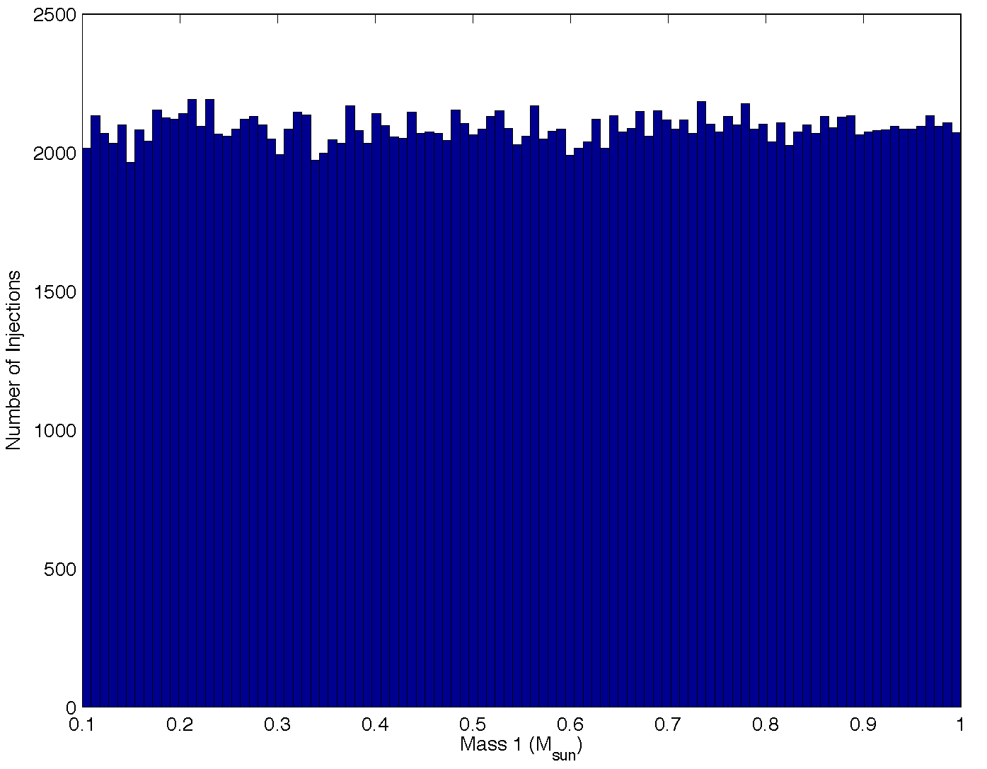
Figure 5: The BBHMACHO population Monte Carlo code is used to simulate a distribution of $209048$ coalescing binaries and a histogram is made of the first component mass, $m_{1}$ to confirm that it is uniformly distributed over the expected range. Similar tests are performed for the second mass parameter, $m_{2}$, the galactocentric longitude, $\theta$, the inclination angle, $\iota$, the polarization angle, $\psi$, and the coalescence phase, $\phi_{c}$.

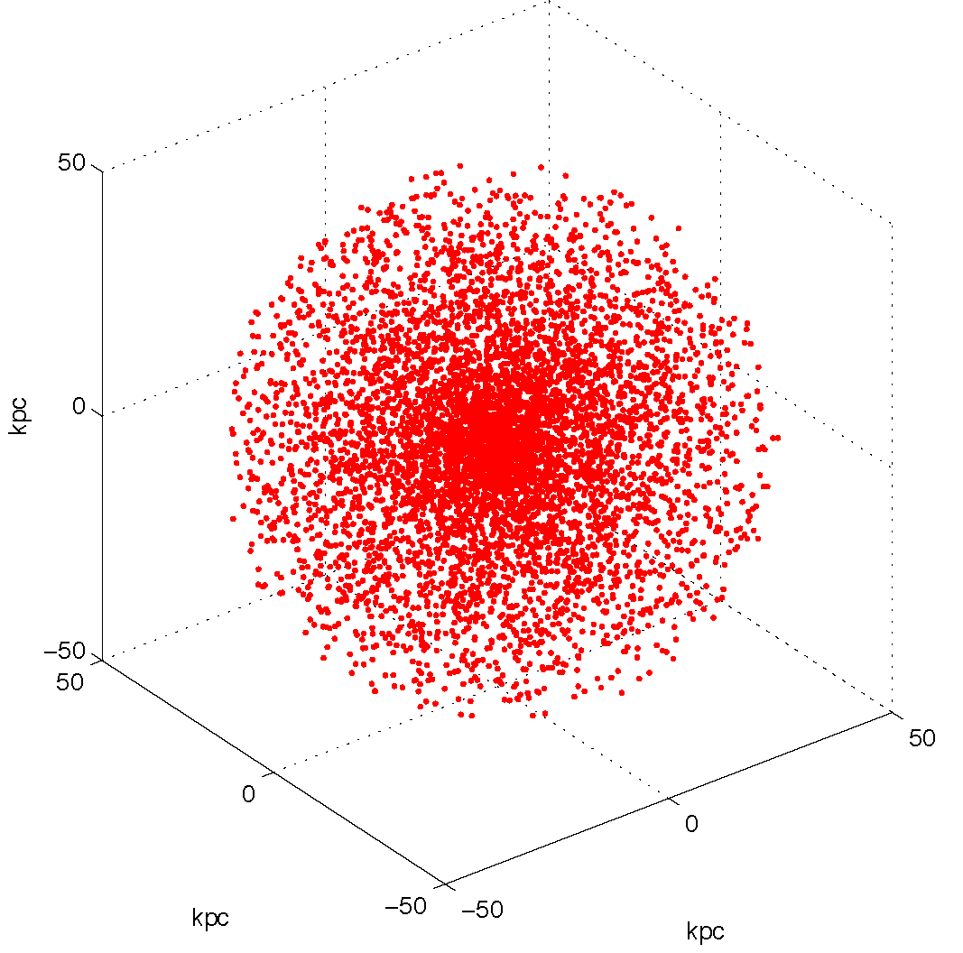
Figure 6: The spatial distribution of $5000$ simulated BBHMACHO binaries in a spherical $q=1$ Galactic halo of size $R_{\mathrm{max}}=50\,\mathrm{kpc}$ with a core radius $a=8.5\,\mathrm{kpc}$ shown in galactocentric coordinates. Each point in the figure corresponds to a simulated binary black hole MACHO injection.

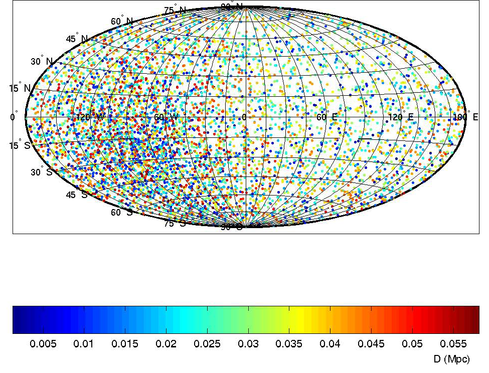
Figure 7: The spatial distribution of $5000$ simulated BBHMACHO binaries in a spherical, $q=0$, Galactic halo of size $R_{\mathrm{max}}=50\,\mathrm{kpc}$ with a core radius $a=8.5\,\mathrm{kpc}$ shown in equatorial coordinates. Each point in the figure corresponds to a simulated binary black hole MACHO injection. The color of the point shows the distance from the center of the earth to the binary. Note the dense clump of binaries in the southern hemisphere, towards the center of the Galaxy.

Chapter 4 Binary Inspiral Search Algorithms

Using equation (2.105)–(2.109), we may write the gravitational wave strain induced in the interferometer as

$$h(t)=\frac{A(t)}{\mathcal{D}}\cos\left(2\phi(t)-\theta\right),$$ (4.1)

where

$$A(t)=-\frac{2G\mu}{c^{4}}\left[\pi GMf(t)\right]^{\frac{2}{3}}$$ (4.2)

and $\mathcal{D}$ is the effective distance, given by

$$\mathcal{D}=\frac{r}{\sqrt{F_{+}^{2}(1+\cos^{2}\iota)^{2}/4+F_{\times}^{2}\cos^{2}\iota}}.$$ (4.3)

The phase angle $\theta$ is

$$\tan\theta=\frac{F_{\times}2\cos\iota}{F_{+}(1+\cos^{2}\iota)}$$ (4.4)

and $\phi(t)$ is given by equation (2.110). In this chapter we address the problem of finding such a signal hidden in detector noise. The detection of signals of known form in noise is a classic problem of signal processing[wainstein:1962] and has been studied in the context of binary inspiral in [Finn:1992wt, Finn:1992xs]. This material is reviewed in section 4.1. The particular implementation used to extract inspiral signals from interferometer data in a computationally efficient manner is presented in section 4.3.

4.1 Detection of Gravitational Waves in Interferometer Noise

Our goal is to determine if the (calibrated) output of the interferometer $s(t)$ contains a gravitational wave in the presence of the detector noise described in section 2.2.2. When the interferometer is operating properly

$$s(t)=\begin{cases}n(t)+h(t)&\text{signal present},\\ n(t)&\text{signal absent}.\end{cases}$$ (4.5)

The instrumental noise $n(t)$ arises from naturally occurring random processes described mathematically by a probability distribution function. The optimum receiver for the signal $h(t)$ takes as input the interferometer data and returns as its output the conditional probability $P(h|s)$ that the signal $h(t)$ is present given the data $s(t)$. The conditional probability that the signal is not present, given the data is then $P(0|s)=1-P(h|s)$. The probabilities $P(h|s)$ and $P(0|s)$ are a posteriori probabilities. They are the result of an experiment to search for the signal $h(t)$. The probability that the signal is present before we conduct the experiment is the a priori probability $P(h)$. Similarly, $P(0)=1-P(h)$ is the a priori probability that the signal is absent.

The construction of the optimal receiver depends on the following elementary probability theory. The probability that two events $A$ and $B$ occur is given by

$$P(A,B)=P(A)P(B|A)=P(B)P(A|B),$$ (4.6)

allowing us to relate the two conditional probabilities by

$$P(A|B)=\frac{P(A,B)}{P(B)}=\frac{P(A)P(B|A)}{P(B)}.$$ (4.7)

If instead of a single event, $A$, suppose we have a complete set of mutually exclusive events $A_{1},A_{2},\ldots,A_{K}$. By mutually exclusive we mean that two or more of these events cannot occur simultaneously and by complete we mean that one of them must occur. Now suppose $B$ is an event that can occur only if one of the $A_{k}$ occurs. Then the probability that $B$ occurs is given by

$$P(B)=\sum_{k=1}^{K}P(A_{k})P(B|A_{k}).$$ (4.8)

Equation (4.8) is called the total probability formula. Now let us suppose that $B$ is the result of an experiment and we want to know the probability that it was event $A_{k}$ that allowed $B$ to happen. This can be obtained by substituting equation (4.8) into equation (4.7) to get

$$P(A_{k}|B)=\frac{P(A_{k})P(B|A_{k})}{P(B)}=\frac{P(A_{k})P(B|A_{k})}{\sum_{j=1}^{K}P(A_{j})P(B|A_{j})}.$$ (4.9)

Equation (4.9) is Bayes’ theorem. The probability $P(A_{k})$ is the a priori probability of event $A_{k}$ occurring and $P(A_{k}|B)$ is the a posteriori probability of $A_{k}$ occurring given that the outcome of our experiment $B$ occurred. The conditional probability $P(B|A_{k})$ is called the likelihood.

Now suppose that set $\{A_{k}\}$ contains only to two members: “the signal is present” and “the signal is absent”. The a priori probabilities of these events are $P(h)$ and $P(0)$, as discussed earlier. We consider $B$ to be the output of the interferometer for a particular experiment. We can use Bayes’ theorem to compute the a posteriori probability that the signal is present, given the output of the detector:

$$P(h|s)=\frac{P(h)P(s|h)}{P(s)}$$ (4.10)

where $P(s)$ is the a priori probability of obtaining the detector output and $P(s|h)$ is the likelihood function. $P(s|h)$ is the probability of obtaining the detector output given that the signal is present in the data. The probability of obtaining the detector output is given by

$$P(s)=P(h)P(s|h)+P(0)P(s|0)$$ (4.11)

since the signal is either present or not present. Substituting equation (4.11) into (4.10), we write

$$P(h|s)=\frac{P(h)P(s|h)}{P(h)P(s|h)+P(0)P(s|0)}.$$ (4.12)

Dividing the numerator and denominator on the right hand side of equation (4.12) by $P(h)P(s|0)$ we obtain

$$P(h|s)=\frac{P(s|h)/P(s|0)}{[P(s|h)/P(s|0)]+[P(0)/P(h)]}.$$ (4.13)

Define the likelihood ratio

$$\Lambda=\frac{P(s|h)}{P(s|0)}$$ (4.14)

so that equation (4.13) becomes

$$P(h|s)=\frac{\Lambda}{\Lambda+[P(0)/P(h)]}.$$ (4.15)

Similarly, we find that the probability that the signal is absent is given by

$$P(0|s)=1-P(h|s)=\frac{P(0)/P(h)}{\Lambda+[P(0)/P(h)]}.$$ (4.16)

Using equations (4.15) and (4.16), we find that the ratio of the a posteriori probabilities is

$$\frac{P(h|s)}{P(0|s)}=\Lambda\frac{P(h)}{P(0)}.$$ (4.17)

We now construct a decision rule for present or absence of the signal. If $P(h|s)$ is large (close to unity) then it is reasonable to conclude that the signal is present. Conversely, if $P(h|s)$ is small (close to zero) then we may conclude that the signal is absent. Therefore we may set a threshold $P_{\ast}$ on this posterior probability as our decision rule is

$$P(h|s) \geq P_{*} \text{decide the signal is present},$$ (4.18)

$$P(h|s) <P_{*} \text{decide the signal is not present}.$$ (4.19)

Given this decision rule there are two erroneous outcomes. If $P(h|s)\geq P_{*}$ and the signal is not present, we call this a false alarm; our decision that the signal is present was incorrect. Conversely, if $P(h|s)<P_{*}$ and the signal is present, we have made a false dismissal. Each possible outcome has an associated probability

$$F$$ probability that we have a false alarm (4.20)

$$F^{\prime} =1-D \text{probability that we have a false dismissal},$$ (4.21)

where $D$ is the probability of a correct detection. To construct the posterior probability, $P(h|s)$ we need the unknown a priori probabilities, $P(h)$ and $P(0)$. We see from equation (4.15), however, that $P(h|s)$ is a monotonically increasing function of the likelihood. The ratio of the a priori probabilities, $P(h)/P(0)$, is a constant that does not involve the result of our experiment. Therefore we can define the output of our optimum receiver to be the device which, given the input data $s(t)$, returns the likelihood ratio $\Lambda$. For the receiver to be optimal in the Neyman-Pearson sense the detection probability should be maximized for a given false alarm rate, $F$. Rule (4.18)–(4.19) is optimal in the Neyman-Pearson sense.

We now consider the construction of $\Lambda$ for the interferometer data $s(t)$ and the gravitational wave signal $h(t)$. Assume that the noise is stationary and Gaussian with zero mean value

$$\left\langle n(t)\right\rangle=0$$ (4.22)

where angle brackets denote averaging over different ensembles of the noise. The (one sided) power spectral density $S_{n}(|f|)$ of the noise is defined by

$$\left\langle\tilde{n}(f)\tilde{n}(f^{\prime})\right\rangle=\frac{1}{2}S_{n}(|f|)\delta(f-f^{\prime})$$ (4.23)

where $\tilde{n}(f)$ is the Fourier transform of $n(t)$. We wish to compute the quantity

$$\Lambda=\frac{P(s|h)}{P(s|0)},$$ (4.24)

however since the probabilities $P(s|h)$ and $P(s|0)$ are usually zero, so in calculating the likelihood ratio, we must get rid of the indeterminacy by writing

$$\Lambda=\frac{P(s|h)}{P(s|0)}=\frac{p(s|h)\,ds}{p(s|0)\,ds}=\frac{p(s|h)}{p(s|0)}.$$ (4.25)

Instead of using the zero probabilities where $P(s|h)$ and $P(s|0)$, we use the corresponding probability densities $p(s|h)$ and $p(s|0)$. The probability density of obtaining a particular instantiation of detector noise is[Finn:1992wt]

$$p(n)=\mathcal{K}\exp\left[-\frac{1}{2}(n|n)\right]$$ (4.26)

where $\mathcal{K}$ is a normalization constant and the inner product $(\cdot|\cdot)$ is given by

$$(a\mid b)\equiv\int_{-\infty}^{\infty}df\,\frac{\tilde{a}^{\ast}(f)\tilde{b}(f)+\tilde{a}(f)\tilde{b}^{\ast}(f)}{S_{n}(|f|)}.$$ (4.27)

The probability density of obtaining the interferometer output, $s(t)$, in the absence of signal, i.e. $s(t)=n(t)$, is therefore

$$p(s|0)=p(s)=\mathcal{K}\exp\left[-\frac{1}{2}(s|s)\right]$$ (4.28)

The probability density of obtaining $s(t)$ in the presence of a signal, i.e. when $s(t)=n(t)+h(t)$, is given by

$$p(s|h)=p(s-h)=\mathcal{K}\exp\left[-\frac{1}{2}(s-h|s-h)\right]$$ (4.29)

where we have used $n(t)=s(t)-h(t)$. Therefore the likelihood ratio becomes

$$\begin{split}\Lambda&=\frac{p(s|h)}{p(s|0)}=\frac{p(s-h)}{p(s)}\\ &=\frac{\exp\left[-\frac{1}{2}(s-h|s-h)\right]}{\exp\left[-\frac{1}{2}(s|s)\right]}\\ &=\exp\left\{-\frac{1}{2}\left[(s|s)-2(s|h)-(h|h)\right]+\frac{1}{2}(s|s)\right\}\\ &=\exp\left[(s|h)-\frac{1}{2}(h|h)\right]\end{split}$$ (4.30)

where $(s|h)$ depends on the detector output and $(h|h)$ is constant for a particular $S_{n}(|f|)$ and $h$. Since the likelihood ratio is a monotonically increasing function of $(s|h)$ we can threshold on $(s|h)$ instead of the posterior probabilities. Our optimal receiver is involves the construction of $(s|h)$ followed by a test

$$\begin{split}(s|h)&\geq x_{\ast}\quad\text{the signal is present},\\ (s|h)&<x_{\ast}\quad\text{the signal is not present}.\end{split}$$ (4.31)

For a given $h(t)$, the inner product in equation (4.27), is a linear map from the infinite dimensional vector space of signals to $\mathbb{R}$. Therefore the optimal receiver is a linear function of the input signal $s(t)$. Both the output of a gravitational wave interferometer and inspiral signals that we are searching for are real functions of time, so

$$\tilde{s}^{\ast}(f) =\tilde{s}(-f)$$ (4.32)

$$\tilde{h}^{\ast}(f) =\tilde{h}(-f)$$ (4.33)

and the inner product in equation (4.27) becomes

$$\left(a\mid b\right)=2\int_{-\infty}^{\infty}df\,\frac{\tilde{a}(f)\tilde{b}^{\ast}(f)}{S_{n}\left(\left|f\right|\right)}.$$ (4.34)

If we receive only noise, then the mean of $(s|h)$ over an ensemble of detector outputs is

$$\begin{split}\left\langle(s|h)\right\rangle&=\left\langle(n|h)\right\rangle\\ &=\int_{-\infty}^{\infty}\frac{\langle\tilde{n}(f)\rangle\tilde{h}^{\ast}(f)}{S_{n}(|f|)}\\ &=0\end{split}$$ (4.35)

since $\langle n(t)\rangle=0$. The variance of $(s|h)$ in the absence of a signal is

$$\begin{split}\left\langle(s|h)^{2}\right\rangle&=4\left\langle\int_{-\infty}^{\infty}\int_{-\infty}^{\infty}\,df\,df^{\prime}\,\frac{\tilde{n}(f)\tilde{h}^{\ast}(f)\tilde{n}^{\ast}(f^{\prime})\tilde{h}(f^{\prime})}{S_{n}(|f|)\,S_{n}(|f^{\prime}|)}\right\rangle\\ &=4\int_{-\infty}^{\infty}\int_{-\infty}^{\infty}\,df\,df^{\prime}\,\frac{\left\langle\tilde{n}(f)\tilde{n}^{\ast}(f^{\prime})\right\rangle\tilde{h}^{\ast}(f)\tilde{h}(f^{\prime})}{S_{n}(|f|)\,S_{n}(|f^{\prime}|)}\\ &=4\int_{-\infty}^{\infty}\int_{-\infty}^{\infty}\,df\,df^{\prime}\,\frac{\frac{1}{2}S_{n}(|f^{\prime}|)\delta(f-f^{\prime})\tilde{h}^{\ast}(f)\tilde{h}(f^{\prime})}{S_{n}(|f|)\,S_{n}(|f^{\prime}|)}\\ &=(h|h)\end{split}$$ (4.36)

where we have used the definition of the one sided power spectral density from equation (4.23). In the presence of signal and noise, then the mean of $(s|h)$ is

$$\left\langle(n+h|h)\right\rangle=(\langle n\rangle+h|h)=(h|h).$$ (4.37)

We can also show that the variance of $(s|h)$ in the presence of a signal is

$$\left\langle\left[(s|h)-(h|h)\right]^{2}\right\rangle=\left\langle\left[(n|h)\right]^{2}\right\rangle=(h|h).$$ (4.38)

Therefore the quantity $(h|h)$ is the variance of the output of the optimal receiver, $(s|h)$, and we denote it by

$$\sigma^{2}\equiv(h|h).$$ (4.39)

Now suppose that the signal we wish to recover has an unknown amplitude, $\mathcal{A}$. The above discussion holds with $h(t)\rightarrow\mathcal{A}h(t)$ and, from equation (4.30), the likelihood ratio becomes

$$\Lambda=\exp\left[\mathcal{A}(s|h)-\frac{1}{2}\mathcal{A}^{2}(h|h)\right]$$ (4.40)

which is again monotonic in $(s|h)$, and so our previous choice of optimal statistic and decision rule hold. Now we are ready to consider the case of a gravitational wave inspiral signal of the form given in equation (4.1). The likelihood ratio now becomes a function of $\theta$

$$\Lambda^{\prime}(\theta)=p(\theta)\exp\left\{D^{-1}(s|A(t)\cos\left[2\phi(t)-\theta\right])-\frac{1}{2}D^{-2}(h|h)\right\}.$$ (4.41)

Now consider the first inner product in the above exponential. Using $\cos(\phi-\theta)=\cos\theta\cos\phi+\sin\theta\sin\phi$, we may write this as

$$\begin{split}\left(s\big{|}A(t)\cos\left[2\phi(t)-\theta\right]\right)&=\cos\theta\left(s\big{|}A(t)\cos\left[2\phi(t)\right]\right)+\sin\theta\left(s\big{|}A(t)\sin\left[2\phi(t)\right]\right)\\ &=x\cos\theta+y\cos\theta\\ &=|z|\cos(\Phi-\theta)\end{split}$$ (4.42)

where

$$x =|z|\cos\Phi=\left(s\big{|}A(t)\cos(2\phi(t))\right),$$ (4.43)

$$y =|z|\sin\Phi=\left(s\big{|}A(t)\sin(2\phi(t))\right),$$ (4.44)

$$|z| =\sqrt{x^{2}+y^{2}},$$ (4.45)

$$\tan\Phi =\frac{y}{x}.$$ (4.46)

(The notation $|z|$ will become clear later in this chapter.) To calculate the likelihood ratio, $\Lambda$, we assume that the unknown phase is uniformly distributed between $0$ and $2\pi$,

$$p(\theta)=\frac{1}{2\pi},$$ (4.47)

and integrate $\Lambda^{\prime}$ over the angle $\theta$ to obtain

$$\begin{split}\Lambda&=\int_{0}^{2\pi}\Lambda^{\prime}(\theta)\,d\theta=\frac{1}{2\pi}\int_{0}^{2\pi}\exp\left[D^{-1}|z|\cos(\Phi-\theta)-\frac{D^{-2}}{2}(h|h)\right]\,d\theta\\ &=I_{0}(D^{-1}|z|)e^{-D^{-2}\frac{1}{2}(h|h)}\end{split}$$ (4.48)

where $I_{0}$ is the modified Bessel function of the first kind of order zero. Once again, we note that the function $I_{0}(D^{-1}|z|)$ is a monotonically increasing function of $|z|$ and so we can threshold on $|z|$ instead of $\Lambda$. Note that $s$ appears in the expression for the likelihood through $|z|$ only.

Recall from chapter 2 that we denoted the two orthogonal phases of the binary inspiral waveform by $h_{c}$ and $h_{s}$ given by equations (2.102) and (2.103)

$$h_{c}(t) =\frac{2}{c^{2}}\left(\frac{\mu}{M_{\odot}}\right)\left[\pi GMf(t)\right]^{\frac{2}{3}}\cos\left[2\phi(t)-2\phi_{0}\right],$$ (4.49)

$$h_{s}(t) =\frac{2}{c^{2}}\left(\frac{\mu}{M_{\odot}}\right)\left[\pi GMf(t)\right]^{\frac{2}{3}}\sin\left[2\phi(t)-2\phi_{0}\right],$$ (4.50)

and so for inspiral waveforms we can compute $|z|$ by

$$z=\sqrt{(s|h_{c})^{2}+(s|h_{s})^{2}}.$$ (4.51)

The threshold on $|z|$ would be determined to achieve a given false alarm probability. We note that in the absence of signal $|z|^{2}$ is the sum of squares of two independent Gaussian random variables of zero means and variance $\sigma^{2}=(h_{c}|h_{c})=(h_{s}|h_{s})$. $x$ and $y$ are independent random variables since $(h_{c}|h_{s})=0$. It is therefore convenient to work with a normalized signal-to-noise ratio defined by

$$\rho^{2}=\frac{|z|^{2}}{\sigma^{2}}$$ (4.52)

which is $\chi^{2}$ distributed with two degrees of freedom for Gaussian detector noise.

If a gravitational wave signal is present, then its location in time is defined by the end time parameter $t_{e}$ of the waveform. In chapter 2 we defined the end time of the chirp to be the time at which the frequency of the gravitational wave reached $f_{\mathrm{isco}}$, taken as the gravitational wave frequency of a particle in the innermost stable circular orbit of Schwarzschild spacetime. In the above discussion of the optimal receiver, we implicitly knew the location of the signal in the data to have $t_{e}=0$. Now suppose that the inspiral waveform ends at some unknown time $t_{e}$. We may write the signal we are searching for as $h(t^{\prime}-t_{e})$. Consider the Fourier transform of this signal

$$\begin{split}\int_{-\infty}^{\infty}e^{-2\pi ift^{\prime}}h(t^{\prime}-t_{e})\,dt^{\prime}&=e^{-2\pi ift_{e}}\int_{-\infty}^{\infty}e^{-2\pi if\tau}h(\tau)\,d\tau\\ &=e^{-2\pi ift_{e}}\tilde{h}(f).\end{split}$$ (4.53)

where we have used $\tau=t^{\prime}-t_{e}$, $dt=d\tau$ and $t^{\prime}=t_{e}+\tau$. The value of the inner product $(s|h_{c})$ for a waveform that ends at time $t_{e}$ is therefore

$$(s|h_{c}(t_{e}))=2\int_{-\infty}^{\infty}\,dfe^{2\pi ift_{e}}\frac{\tilde{s}(f)\tilde{h}_{c}^{\ast}(f)}{S_{n}(|f|)}$$ (4.54)

and the signal-to-noise ratio for a chirp that ends at time $t$ is

$$\rho(t)=\frac{1}{\sigma}\sqrt{(s|h_{c}(t))^{2}+(s|h_{s}(t))^{2}}$$ (4.55)

where the quantities $(s|h_{c}(t))$ and $(s|h_{s}(t))$ can be obtained by inverse Fourier transforms of the form in equation (4.54).

Now the statistic $\rho(t)$ derived from the likelihood is a function of a time parameter. For Neyman-Pearson optimal detection, we would integrate over all possible arrival times and threshold on this value. However, as well as making a statement about the presence or absence of a signal in the data we also want to measure the time that the signal occurs. To do this, we use the method of maximum likelihood[helstrom:1995]. The maximum likelihood estimator states that the most probable value for the location of the signal is the time at which the likelihood ratio is maximized. So to find a single inspiral signal in a segment of interferometer data, we search for the maximum of $\rho(t)$. If $\max_{t}\left[\rho(t)\right]>\rho_{\ast}$ then we decide that we have detected a signal at the time of the maximum. When there is more than one inspiral in the data segment the maximization is not over all times.

We have now completely specified the solution to the problem of finding a waveform of unknown amplitude and phase at an unknown time in the data; our optimum receiver is the matched filter of equation equation (4.54). Below we develop the formalism to construct a digital implementation of the matched filter to search for gravitational wave signals in interferometer data.

4.2 Conventions for Discrete Quantities

The raw output of the interferometer is the error signal from the length sensing and control servo, LSC-AS_Q, as described in chapter 2. Although this signal is a dimensionless quantity, we say that it has units of “counts” and we denote it by $v(t)$. The calibrated detector output is related to the raw detector output by the detector response function according to

$$\tilde{s}(f)=R(f;t)\tilde{v}(f)$$ (4.56)

where $R(f;t)$ is the (complex) response function of the detector at time $t$ and has units of strain/count (see section 2.2.3). In practice, the interferometer output is a discretely sampled quantity with sampling interval $\Delta t$, that is $v_{j}\equiv v(t_{j})$ where $t_{j}=j\Delta t$. The digital matched filter operates on a single data segment consisting of $N$ consecutive samples of $v(t_{j})$. The length of this data segment is $T=N\Delta t$ seconds. Henceforth, we let $N$ be a power of $2$ and follow the convention that the subscript $j$ refers to discretely sampled time domain quantities and the subscript $k$ to discretely sampled frequency domain quantities. The frequency domain quantity $\tilde{v}(f_{k})$ denotes the value of the continuous function $\tilde{v}(f)$ at a particular frequency, labeled $f_{k}=k/(N\Delta t)$. If the units of $v_{j}$ are counts, then $\tilde{v}(f_{k})$ has units of counts/Hz. We define the quantity $\tilde{v}_{k}$ by $\tilde{v}_{k}=\tilde{v}(f_{k})/\Delta t$, which has units of counts. If $k$ is negative, this corresponds to negative frequencies.

4.2.1 The Discrete Fourier Transform

If $v(t_{j})$ is sampled at intervals of $\Delta t$, then the sampling theorem[Press:1992] tells us that $v(t_{j})$ is bandwidth limited to the frequency range $-f_{\mathrm{Ny}}\leq f\leq f_{\mathrm{Ny}}$, where

$$f_{\mathrm{Ny}}=\frac{1}{2\Delta t}$$ (4.57)

is the Nyquist critical frequency. Any power in $v(t)$ at frequencies above $f_{\mathrm{Ny}}$ will be aliased into the range $-f_{\mathrm{Ny}}\leq f\leq f_{\mathrm{Ny}}$, corrupting the signal. To prevent this, signals of frequency higher than $f_{\mathrm{Ny}}$ in the interferometer output are removed using analog low-pass filters before the signal is digitized. Therefore $v(t_{j})$ completely determines the signal $v(t)$ in the band of interest. We may approximate the Fourier transform of this band limited signal $v(t_{j})$ by

$$\tilde{v}(f_{k})\rightsquigarrow\sum_{j=0}^{N-1}\Delta t\,v(t_{j})e^{-2\pi if_{k}t_{j}}=\Delta t\sum_{j=0}^{N-1}v_{j}e^{-2\pi ijk/N},$$ (4.58)

where $-(N/2+1)\leq k\leq N/2$ and the symbol $\rightsquigarrow$ means equal to under discretization. Notice that the approximation to the Fourier transform is periodic in $k$ with period $N$ and so

$$\tilde{v}_{-k}=\tilde{v}_{N-k}\quad k=1,\ldots,N-1.$$ (4.59)

Thus we let $k$ vary from $0$ to $N-1$ where zero frequency (DC) corresponds to $k=0$, positive frequencies $0<f<f_{\mathrm{Ny}}$ to values in the range $0<k<N/2$ and negative frequencies $-f_{\mathrm{Ny}}<f<0$ correspond to values in the range $N/2<k<N$. The value $k=N/2$ approximates the value of the Fourier transform at both $-f_{\mathrm{Ny}}$ and $f_{\mathrm{Ny}}$; both these values are equal due to the periodicity of the discrete transform defined by[Anderson:2001a]

$$\tilde{v}_{k}=\sum_{j=0}^{N-1}v_{j}e^{-i2\pi jk/N}.$$ (4.60)

We may estimate the discrete inverse Fourier transform in a similar way, using the relation

$$\Delta f=f_{k+1}-f_{k}=\frac{k+1}{N\Delta t}-\frac{k}{N\Delta t}=\frac{1}{N\Delta t}$$ (4.61)

to obtain

$$v_{j}=\frac{1}{N}\sum_{k=0}^{N-1}\tilde{v}_{k}e^{2\pi ijk/N}.$$ (4.62)

4.2.2 Power Spectral Densities

In equation (4.23), we defined the one sided power spectral density $S_{n}(|f|)$ of $n(t)$ to be

$$\left\langle\tilde{n}(f)\tilde{n}^{\ast}(f^{\prime})\right\rangle=\frac{1}{2}S_{n}(|f|)\delta(f-f^{\prime})$$ (4.63)

where angle brackets denote an average over different realizations of the noise. If $n(t)$ has units of $U$ then $\tilde{n}(f)$ has units of $(\mathrm{time})\times U$. The units $\delta(f-f^{\prime})$ are $(\mathrm{time})$, since

$$\int_{-\infty}^{\infty}\delta(f)\,df=1$$ (4.64)

is a dimensionless quantity and $df$ has units $(\mathrm{time})^{-1}$. Therefore we see that $S_{n}(|f|)$ has units of $(\mathrm{time})\times U^{2}$. If we replace $\tilde{n}(f_{k})$ with the discretely sampled quantities $\tilde{n}_{k}=\tilde{n}(f_{k})$, we obtain

$$\left\langle\tilde{n}_{k}\tilde{n}_{k^{\prime}}^{\ast}\right\rangle=\frac{N}{2\Delta t}S_{n}\left(\left|f_{k}\right|\right)\delta_{kk^{\prime}}$$ (4.65)

where $\delta_{kk^{\prime}}$ is the dimensionless Kronecker $\delta$-function, obtained by discretization of the continuous $\delta$-function:

$$\delta(f-f^{\prime})\rightsquigarrow N\Delta t\delta_{kk^{\prime}}$$ (4.66)

Equation (4.65) defines $S_{n}\left(\left|f_{k}\right|\right)$in terms of the discrete frequency domain quantities. The definition in equation (4.65) is equivalent to

$$S_{n}\left(\left|f_{k}\right|\right)=\begin{cases}\frac{\Delta t}{N}\left\langle|\tilde{n}_{0}|^{2}\right\rangle&k=0,\\ \frac{\Delta t}{N}\left\langle|\tilde{n}_{N/2}|^{2}\right\rangle&k=\frac{N}{2},\\ \frac{\Delta t}{N}\left\langle\left(|\tilde{n}_{k}|^{2}+|\tilde{n}_{N-k}|^{2}\right)\right\rangle&\text{otherwise}\end{cases}$$ (4.67)

where the normalization is chosen so that the power spectral density satisfies the discrete form of Parseval’s theorem

$$\Delta t\sum_{j=0}^{N-1}|v_{j}|^{2}=\sum_{k=0}^{N/2}S_{v}(f_{k}).$$ (4.68)

Parseval’s theorem states that the total power in a signal is independent of whether it is calculated in the time domain or the frequency domain.

The value of $S_{n}\left(\left|f_{k}\right|\right)$for white Gaussian noise will be useful to us later, so we compute it here. If the noise $n(t)$ is zero mean, white noise with variance $\varsigma^{2}$, then

$$\begin{split}\left\langle\tilde{n}_{k}\tilde{n}_{k^{\prime}}^{\ast}\right\rangle&=\sum_{j=0}^{N-1}\sum_{j^{\prime}=0}^{N-1}e^{2\pi i\left(jk-j^{\prime}k^{\prime}\right)/N}\left\langle n_{j}n_{j^{\prime}}\right\rangle\\ &=\sum_{j=0}^{N-1}\sum_{j^{\prime}=0}^{N-1}e^{2\pi i\left(jk-j^{\prime}k^{\prime}\right)/N}\varsigma^{2}\delta_{jj^{\prime}}\\ &=\sum_{j=0}^{N-1}e^{2\pi ij\left(k-k^{\prime}\right)/N}\varsigma^{2}\\ &=N\delta_{kk^{\prime}}\varsigma^{2}\end{split}$$ (4.69)

Substituting this into equation (4.65), we obtain

$$\frac{N}{2\Delta t}S_{n}\left(\left|f_{k}\right|\right)\delta_{kk^{\prime}}=N\delta_{kk^{\prime}}\varsigma^{2}$$ (4.70)

and so the power spectrum of white Gaussian noise is a constant with value

$$S_{n}\left(\left|f_{k}\right|\right)=2\Delta t\varsigma^{2}.$$ (4.71)

4.3 Digital Matched Filtering

The signal-to-noise ratio (4.52) requires us to compute the time series

$$x(t)=2\int_{-\infty}^{\infty}df\,e^{2\pi ift}\frac{\tilde{s}(f)\tilde{h_{c}}^{\ast}(f)}{S_{n}\left(\left|f\right|\right)}$$ (4.72)

and

$$y(t)=2\int_{-\infty}^{\infty}df\,e^{2\pi ift}\frac{\tilde{s}(f)\tilde{h_{s}}^{\ast}(f)}{S_{n}\left(\left|f\right|\right)}$$ (4.73)

and the normalization constant $\sigma$ that measures that “amount of noise” in the detector (for a given inspiral waveform). From the definition of the inner product in equation (4.34) and the definition of $\sigma^{2}$ in equation (4.39), we explicitly write

$$\sigma^{2}=2\int_{-\infty}^{\infty}df\,\frac{\tilde{h_{c}}^{\ast}(f)\tilde{h_{c}}(f)}{S_{h}\left(\left|f\right|\right)}=2\int_{-\infty}^{\infty}\frac{\tilde{h_{s}}^{\ast}(f)\tilde{h_{s}}(f)}{S_{h}\left(\left|f\right|\right)}.$$ (4.74)

The signal-to-noise ratio is normalized according to the convention of Cutler and Flanagan [Cutler:1994], so that in the case when the detector output is Gaussian noise, the square of the signal-to-noise ratio averaged over an ensemble of detectors with different realizations of the noise is

$$\left\langle\rho^{2}\right\rangle=\frac{1}{\sigma^{2}}\left\langle x^{2}+y^{2}\right\rangle=2,$$ (4.75)

as seen from equation (4.36).

4.3.1 Construction of the digital filter using stationary phase chirps

In section 2.3.2 we derived the stationary phase approximation to the Fourier transform of the restricted post²-Newtonian binary inspiral waveform to be

$$\tilde{h}_{c}(f) =\frac{2GM_{\odot}}{(1\,\mathrm{Mpc})c^{2}}\left(\frac{5\mu}{96M_{\odot}}\right)^{\frac{1}{2}}\left(\frac{M}{\pi^{2}M_{\odot}}\right)^{\frac{1}{3}}f^{-\frac{7}{6}}\,\left(\frac{GM_{\odot}}{c^{3}}\right)^{-\frac{1}{6}}\,e^{i\Psi(f;M,\eta)},$$ (4.76)

$$\tilde{h}_{s}(f) =i\tilde{h}_{c}(f),$$ (4.77)

where $f$ is the gravitational wave frequency in Hz, $M=m_{1}+m_{2}$ is the total mass of the binary measured in solar masses, $\mu=m_{1}m_{2}/M$ is the reduced mass and $\eta=\mu/M$. Note that $\tilde{h}_{c,s}(f)$ have units of 1/Hz and we have chosen the chirp to be at a canonical distance of $r=1\,\mathrm{Mpc}$. The instrument strain per Hz $\tilde{h}(f)$ is a linear superposition of $\tilde{h}_{c,s}(f)$ in the same way as $h(t)$ is obtained from $h_{c,s}(t)$. The phase evolution to post²-Newtonian order is given by

$$\begin{split}\Psi(f;M,\eta)&=2\pi ft_{c}-2\phi_{0}-\pi/4+\frac{3}{128\eta}\biggl{[}x^{-5}+\left(\frac{3715}{756}+\frac{55}{9}\eta\right)x^{-3}-16\pi x^{-2}\\ &\quad+\left(\frac{15\,293\,365}{508\,032}+\frac{27\,145}{504}\eta+\frac{3085}{72}\eta^{2}\right)x^{-1}\biggr{]},\end{split}$$ (4.78)

where $x=(\pi MfG/c^{3})^{1/3}$. The coalescence phase $\phi_{0}$ is the orbital phase, determined by the binary ephemeris, and the coalescence time $t_{c}$ is the time at which the bodies collide. The overall value coalescence phase $\phi_{0}$ is part of the unknown phase of the matched filter and we set $\phi_{0}=0$, respectively. We set the coalescence time $t_{c}=0$, since it is accounted for by the Fourier transform in equations (4.72) and (4.73). The validity of the stationary phase approximation for inspiral templates is well established[Droz:1999qx].

Since the two chirp waveforms $\tilde{h_{c}}$ and $\tilde{h_{s}}$ are orthogonal, the most efficient algorithm for constructing the time series $\rho(t)$ uses a single complex inverse FFT rather than computing it from $x(t)$ and $y(t)$ which requires two real inverse FFTs. We may further increase efficiency when using stationary phase chirps by splitting the filter into a part that depends on the data and a part that depends only on the template parameters. In this section we describe the construction of a digital matched filter which uses these two tricks. Consider the discrete form of equation (4.72)

$$\begin{split}x_{j}&=2\frac{1}{N\Delta t}\sum_{k=0}^{N-1}e^{2\pi ijk/N}\frac{\tilde{s}(f_{k})\tilde{h}_{c}^{\ast}(f_{k})}{S_{n}\left(\left|f_{k}\right|\right)}\\ &=2\frac{\Delta t}{N}\sum_{k=0}^{N-1}e^{2\pi ijk/N}\frac{\tilde{s}_{k}\tilde{h}_{ck}^{\ast}}{S_{n}\left(\left|f_{k}\right|\right)}\end{split}$$ (4.79)

where $\tilde{h}_{ck}\equiv{h}_{c}(f_{k})/\Delta t$. From equation (4.73) we obtain

$$y_{j}=2\frac{\Delta t}{N}\sum_{k=0}^{N-1}e^{2\pi ijk/N}\frac{\tilde{s}_{k}\tilde{h}_{sk}^{\ast}}{S_{n}\left(\left|f_{k}\right|\right)}.$$ (4.80)

Recall that $s(t)$ and $h(t)$ are real signals. We may use the relations $\tilde{s}(f)=\tilde{s}^{\ast}(-f)$ and $\tilde{h}(f)=\tilde{h}^{\ast}(-f)$ to write the normalization constant, $\sigma^{2}$, defined in equation (4.74), as

$$\begin{split}\sigma^{2}&=2\frac{1}{N\Delta t}\sum_{k=0}^{N-1}\frac{\tilde{h}_{c}(f_{k})\tilde{h}_{c}^{\ast}(f_{k})}{S_{n}\left(\left|f_{k}\right|\right)}\\ &=2\frac{\Delta t}{N}\sum_{k=0}^{N-1}\frac{\tilde{h}_{ck}\tilde{h}_{ck}^{\ast}}{S_{n}\left(\left|f_{k}\right|\right)}\\ &=2\frac{\Delta t}{N}\left(\frac{\tilde{h}_{c0}\tilde{h}_{c0}^{\ast}}{S_{n}\left(\left|f_{k}\right|\right)}+2\sum_{k=1}^{N/2-1}\frac{\tilde{h}_{ck}\tilde{h}_{ck}^{\ast}}{S_{n}\left(\left|f_{k}\right|\right)}+\frac{\tilde{h}_{cN/2}\tilde{h}_{cN/2}^{\ast}}{S_{n}\left(\left|f_{k}\right|\right)}\right).\end{split}$$ (4.81)

Since earth based gravitational wave detectors have no useful low frequency response, henceforth we set the DC ($k=0$) term to zero. In addition to this, we assume that there is no power at the Nyquist frequency, as the low pass filter that band limits the interferometer data to frequencies below $f_{\mathrm{Ny}}$ falls off rapidly as the Nyquist frequency is approached. Therefore we may also set the $k=N/2$ term to zero. We assume this for all frequency domain quantities.

Now we may write the cosine phase of the filter given in equation (4.79) as

$$\begin{split}x_{j}&=2\frac{\Delta t}{N}\left[\sum_{k=N/2+1}^{N-1}e^{2\pi ijk/N}\frac{\tilde{s}_{k}\tilde{h}_{ck}^{\ast}}{S_{n}\left(\left|f_{k}\right|\right)}+\sum_{k=1}^{N/2-1}e^{2\pi ijk/N}\frac{\tilde{s}_{k}\tilde{h}_{ck}^{\ast}}{S_{n}\left(\left|f_{k}\right|\right)}\right]\\ &=2\frac{\Delta t}{N}\left[\sum_{k=1}^{N/2-1}e^{-2\pi ijk/N}\frac{\tilde{s}_{k}^{\ast}\tilde{h}_{ck}}{S_{n}\left(\left|f_{k}\right|\right)}+\sum_{k=1}^{N/2-1}e^{2\pi ijk/N}\frac{\tilde{s}_{k}\tilde{h}_{ck}^{\ast}}{S_{n}\left(\left|f_{k}\right|\right)}\right]\\ &=2\frac{\Delta t}{N}(Q_{j}^{\ast}+Q_{j})\end{split}$$ (4.82)

where we have used the fact that $f_{k}=f_{N-k}$. $Q_{j}$ is defined to be

$$Q_{j}=\sum_{k=1}^{N/2-1}e^{2\pi ijk/N}\frac{\tilde{s}_{k}\tilde{h}_{ck}^{\ast}}{S_{n}\left(\left|f_{k}\right|\right)}.$$ (4.83)

The sine phase of the filter given in equation (4.80) can similarly be written as

$$\begin{split}y_{j}&=2\frac{\Delta t}{N}\left[\sum_{k=N/2+1}^{N-1}e^{2\pi ijk/N}\frac{\tilde{s}_{k}\tilde{h}_{sk}^{\ast}}{S_{n}\left(\left|f_{k}\right|\right)}+\sum_{k=1}^{N/2-1}e^{2\pi ijk/N}\frac{\tilde{s}_{k}\tilde{h}_{sk}^{\ast}}{S_{n}\left(\left|f_{k}\right|\right)}\right]\\ &=2\frac{\Delta t}{N}\left[\sum_{k=1}^{N/2-1}e^{-2\pi ijk/N}\frac{\tilde{s}_{k}^{\ast}\tilde{h}_{sk}}{S_{n}\left(\left|f_{k}\right|\right)}+\sum_{k=1}^{N/2-1}e^{2\pi ijk/N}\frac{\tilde{s}_{k}\tilde{h}_{sk}^{\ast}}{S_{n}\left(\left|f_{k}\right|\right)}\right].\end{split}$$ (4.84)

Using $\tilde{h}_{s}=i\tilde{h}_{c}$, equation (4.84) becomes

$$\begin{split}y_{j}&=2\frac{\Delta t}{N}\left[\sum_{k=1}^{N/2-1}e^{-2\pi ijk/N}\frac{\tilde{s}_{k}^{\ast}i\tilde{h}_{ck}}{S_{n}\left(\left|f_{k}\right|\right)}+\sum_{k=1}^{N/2-1}e^{2\pi ijk/N}\frac{\tilde{s}_{k}(-i)\tilde{h}_{ck}^{\ast}}{S_{n}\left(\left|f_{k}\right|\right)}\right]\\ &=-2i\frac{\Delta t}{N}\left[-\sum_{k=1}^{N/2-1}e^{-2\pi ijk/N}\frac{\tilde{s}_{k}^{\ast}\tilde{h}_{ck}}{S_{n}\left(\left|f_{k}\right|\right)}+\sum_{k=1}^{N/2-1}e^{2\pi ijk/N}\frac{\tilde{s}_{k}\tilde{h}_{ck}^{\ast}}{S_{n}\left(\left|f_{k}\right|\right)}\right]\\ &=2\frac{\Delta t}{N}i(Q_{j}^{\ast}-Q_{j}).\end{split}$$ (4.85)

Thus the outputs of the filter for the two phases are

$$x_{j} =\Re z_{j},$$ (4.86)

$$y_{j} =\Im z_{j}.$$ (4.87)

The quantity $z_{j}$ is defined to be

$$\begin{split}z_{j}&=4\frac{\Delta t}{N}\sum_{k=1}^{N/2-1}e^{2\pi ijk/N}\frac{\tilde{s}_{k}\tilde{h}_{ck}^{\ast}}{S_{n}\left(\left|f_{k}\right|\right)}\\ &=\frac{\Delta t}{N}\sum_{k=0}^{N-1}e^{2\pi ijk/N}\tilde{z}_{k}\end{split}$$ (4.88)

where

$$\tilde{z}_{k}=\left\{\begin{array}[]{ll}4\frac{\tilde{s}_{k}\tilde{h}_{ck}^{\ast}}{S_{n}\left(\left|f_{k}\right|\right)}&0<k<\frac{N}{2},\\ \\ 0&\mathrm{otherwise}.\end{array}\right.$$ (4.89)

We can now compute the square of the signal-to-noise ratio

$$\rho^{2}(t_{j})=\frac{x_{j}^{2}+y_{j}^{2}}{\sigma^{2}}=\frac{1}{\sigma^{2}}|z_{j}|^{2}$$ (4.90)

by a single complex inverse Fourier transform and threshold on $\rho^{2}\geq\rho^{2}_{\ast}$. Since we choose the template $\tilde{h}_{c}(f)$ to be at a canonical distance of $1$ Mpc, the effective distance $\mathcal{D}$ to a chirp detected with signal to noise ratio $\rho^{2}$ can be established as

$$\mathcal{D}=\frac{\sigma}{\rho}\,\mathrm{Mpc}.$$ (4.91)

Recall that $\sigma$ is a measure of the noise in the interferometer output; it is a measure of the sensitivity of the detector. Larger values of $\sigma$ correspond to a quieter detector (due to the $1/S_{n}\left(\left|f_{k}\right|\right)$ term in the expression for $\sigma$) and smaller values to a noisier detector.

4.3.2 Details of Filter Implementation

The calibrated detector output is related to the raw detector output by the detector response function according to

$$\tilde{s}(f)=R(f;t)\tilde{v}(f)$$ (4.92)

where $R(f;t)$ is the (complex) response function of the detector at a specific time $t$, as described in chapter 2. In practice, we compute the uncalibrated power spectral density $S_{v}(|f_{k}|)$ from the raw data and then the calibrated power spectral density, $S_{n}\left(\left|f_{k}\right|\right)$, in the denominator of (4.88) is

$$S_{n}\left(\left|f_{k}\right|\right)=|R(f;t)|^{2}S_{v}(|f_{k}|).$$ (4.93)

Further details of the computation of $S_{v}(|f_{k}|)$ are given in sections 4.6 and 4.7.

Typical values of the variance of $v(t)$ for initial LIGO data are $10^{3}$; however, the response function $R(f)$ has magnitude $\sim 10^{-22}$ at the most sensitive frequencies of the instrument. This means that $S_{n}\left(\left|f_{k}\right|\right)\sim 10^{-44}$ which is beyond the range of 4-byte floating point numbers. We may store such values as 8-byte floating point numbers, but this is wasteful of memory since the extra precision of an 8-byte number is not needed. Therefore when we implement the digital filter, we multiply the response function $R(f)$ by a scaling variable $d$ which typically has values of $d=2^{69}$ for initial LIGO data. This scales all frequency domain quantities to have approximately order unity. Therefore equation (4.88) becomes

$$z_{j}=4\frac{\Delta t}{N}\sum_{k=1}^{N/2-1}e^{2\pi ijk/N}\frac{dR\tilde{v}_{k}\,d\tilde{h}_{ck}^{\ast}}{d^{2}|R|^{2}S_{v}\left(\left|f_{k}\right|\right)}$$ (4.94)

and (4.81) becomes

$$\sigma^{2}=4\frac{\Delta t}{N}\sum_{k=1}^{N/2-1}\frac{d^{2}\tilde{h}_{ck}\tilde{h}_{ck}^{\ast}}{d^{2}|R|^{2}S_{v}\left(\left|f_{k}\right|\right)}.$$ (4.95)

Notice that we must also multiply the chirp by $d$ so that all the factors of $d$ cancel in the signal-to-noise ratio $\rho(t_{j})$ and the normalization constant $\sigma^{2}$. In fact this is convenient as it brings the value of the $\tilde{h}_{c}(f_{k})$ to order unity for chirps that would produce a signal-to-noise ratio of order unity. From equation (4.76) we obtain the dimensionless quantity

$$\begin{split}d\,\tilde{h}_{ck}&=\frac{d\tilde{h}_{c}(f_{k})}{\Delta t}\\ &=\frac{2dGM_{\odot}}{(1\,\mathrm{Mpc})c^{2}}\left(\frac{5\mu}{96M_{\odot}}\right)^{\frac{1}{2}}\left(\frac{M}{\pi^{2}M_{\odot}}\right)^{\frac{1}{3}}\left(\frac{GM_{\odot}}{c^{3}\Delta t}\right)^{-\frac{1}{6}}\left(f\,\Delta t\right)^{-\frac{7}{6}}\\ &\quad\quad\times\exp\,[i\Psi(f_{k};M,\eta)]\Theta\left(k-k_{\mathrm{isco}}\right)\\ &=\sqrt{\mathcal{T}(M,\mu)}\left(\frac{k}{N}\right)^{-\frac{7}{6}}e^{i\Psi\left(f_{k};M,\eta\right)}\Theta\left(k-k_{\mathrm{isco}}\right)\end{split}$$ (4.96)

where the term $\Theta\left(k-k_{\mathrm{isco}}\right)$ ensure that the chirp is terminated at the frequency of the innermost stable circular orbit of Schwarzschild. The function $\Psi(f_{k};M,\eta)$ is the value of the post²-Newtonian phase evolution, which is given by (4.78), at the frequency $f_{k}$. The quantity $\mathcal{T}(M,\mu)$ in equation (4.96) is called the template dependent normalization constant and is given by

$$\mathcal{T}(M,\mu)=\left[\left(\frac{2dGM_{\odot}}{(1\,\mathrm{Mpc})c^{2}}\right)\left(\frac{5\mu}{96M_{\odot}}\right)^{\frac{1}{2}}\left(\frac{M}{\pi^{2}M_{\odot}}\right)^{\frac{1}{3}}\left(\frac{GM_{\odot}}{\Delta tc^{3}}\right)^{-\frac{1}{6}}\right]^{2}.$$ (4.97)

Note that $\mathcal{T}(M,\eta)$ depends on the masses of the template and as such must be recomputed once per template. If we substitute equation (4.96) into equation (4.95) we obtain

$$\sigma^{2}=4\frac{\Delta t}{N}\mathcal{T}\sum_{k=1}^{k_{\mathrm{isco}}}\frac{\left(\frac{k}{N}\right)^{-\frac{7}{3}}}{d^{2}|R|^{2}S_{v}\left(\left|f_{k}\right|\right)}=4\frac{\Delta t}{N}\mathcal{T}\mathcal{S}$$ (4.98)

where $\mathcal{S}$ is defined to be

$$\mathcal{S}=\sum_{k=1}^{k_{\mathrm{isco}}}\frac{\left(\frac{k}{N}\right)^{-\frac{7}{3}}}{d^{2}|R|^{2}S_{v}\left(\left|f_{k}\right|\right)}.$$ (4.99)

$\mathcal{S}$ is referred to as the segment dependent normalization. It depends on the binary masses only through $k_{\mathrm{isco}}$, so we compute and store the array

$$\mathcal{S}(k_{\mathrm{isco}})\quad\quad 1\leq k_{\mathrm{isco}}\leq\frac{N}{2}$$ (4.100)

from the input power spectral density. We then select the correct value of $\mathcal{S}$ for a given mass pair by computing $k_{\mathrm{isco}}=f_{\mathrm{isco}}/\Delta f$.

The signal-to-noise ratio squared is then

$$\rho^{2}(t_{j})=\frac{16}{\sigma^{2}}\left(\frac{\Delta t}{N}\right)^{2}\mathcal{T}\left|\sum_{k=1}^{N/2-1}e^{2\pi ijk/N}\frac{dR\tilde{v}_{k}\left(\frac{k}{N}\right)^{-\frac{7}{6}}e^{-i\Psi(f_{k};M,\eta)}\Theta(k-k_{\mathrm{isco}})}{d^{2}|R|^{2}S_{v}\left(\left|f_{k}\right|\right)}\right|^{2}$$ (4.101)

where $\sigma^{2}$ is now given by equation (4.98). Let us define $\tilde{q}_{k}$ by

$$\tilde{q}_{k}=\begin{cases}\frac{d\tilde{v}_{k}\left(\frac{k}{N}\right)^{-\frac{7}{6}}\exp\left[-i\Psi(f_{k};M,\eta)\right]}{d^{2}|R|^{2}S_{v}\left(\left|f_{k}\right|\right)}&0<k<k_{\mathrm{isco}},\\ 0&\text{otherwise}.\end{cases}$$ (4.102)

and $q_{j}$ as the discrete complex inverse Fourier transform of $\tilde{q}_{k}$. Then the signal-to-noise ratio squared is

$$\rho^{2}(t_{j})=\frac{16}{\sigma^{2}}\left(\frac{\Delta T}{N}\right)^{2}\mathcal{T}\left|q_{j}\right|^{2}$$ (4.103)

The computation of $\tilde{q}_{k}$ can further be split into the template independent computation of

$$\tilde{F}_{k}=\frac{d\tilde{v}_{k}\left(\frac{k}{N}\right)^{-\frac{7}{6}}}{d^{2}|R|^{2}S_{v}\left(\left|f_{k}\right|\right)}$$ (4.104)

and the computation of

$$\tilde{T}_{k}=\exp\left[i\Psi(f_{k};M,\eta)\right]\Theta\left(k-k_{\mathrm{isco}}\right)$$ (4.105)

where $\tilde{F}_{k}$ is called the findchirp data segment and $\tilde{T}_{k}$ is called the findchirp template, so

$$\tilde{q}_{k}=\begin{cases}\tilde{F}_{k}\tilde{T}_{k}^{\ast}&0<k<\frac{N}{2},\\ 0&\text{otherwise}.\end{cases}$$ (4.106)

The goal of this separation is to reduce the computational cost of producing $\rho(t)$ by computing the template and using it to filter several data segments. For a given power spectral density $S_{v}(|f_{k}|)$ we only need to compute $\mathcal{S}(k_{\mathrm{isco}})$ once. The findchirp code is designed to process several data segments, labeled $i=1,\ldots,M$, at a time. We can compute $\tilde{F}_{k}^{i}$ once for each data segment and then for each template we compute $\mathcal{T}$ and $\tilde{T}_{k}$. This reduces the computational cost of filter generation. Furthermore, we can threshold against the quantity $|q_{j}|^{2}$

$$|q|^{2}_{\ast}=\frac{\rho^{2}_{\ast}}{\frac{16}{\sigma^{2}}\left(\frac{\Delta t}{N}\right)^{2}\mathcal{T}}$$ (4.107)

thus saving a multiplication per sample point. The effective distance of an inspiral signal at time $t_{j}=j\Delta t$ is given by equation (4.91) which becomes

$$\mathcal{D}=\frac{\mathcal{T}\mathcal{S}^{2}}{|q_{j}|^{2}}$$ (4.108)

in this notation.

4.3.3 Recording Triggers

We call times when the optimal receiver tells us that a signal is present inspiral triggers and record the time of the trigger, the mass parameters of the template and the value of $\sigma^{2}$ for the data segment. There are several complications that mean that simply thresholding on equation (4.107) is not what we do in practice, however. In section 4.4.2 we will show that an impulse in the data segment can cause the filter output event though no chirp is present, and hence cause a false alarms. Although such events are rare in Gaussian noise, they are quite common in real detector output, so we construct an addition test on the presence of absence of the signal, called the $\chi^{2}$ veto[Allen:2004], which is described in section 4.8. Furthermore, the inspiral signals that we are searching for are shorter than the length of a data segment, so we want to allow the possibility of generating multiple inspiral triggers in a single data segment. We also do not record all times for which $|q_{j}|^{2}\geq|q|^{2}_{\ast}$, as we would soon be flooded with triggers in real interferometer data. The algorithm that we use to select the times for which we generate inspiral triggers based on the output of the matched filter and the $\chi^{2}$ veto is described in section 4.9.

4.4 Testing the filtering code

4.4.1 Normalization

Consider the case when the filter input is Gaussian noise, i.e. $\tilde{s}_{k}=\tilde{n}_{k}$ and set $R(f_{k})\equiv 1$ and $d=1$. Then the expectation value of the signal-to-noise ratio squared, $\langle\rho^{2}\rangle$ is

$$\begin{split}\langle\rho^{2}(t_{j})\rangle&=\frac{16}{\sigma^{2}}\left(\frac{\Delta t}{N}\right)^{2}\mathcal{T}\sum_{k=1}^{k_{\mathrm{isco}}}\sum_{k^{\prime}=1}^{k_{\mathrm{isco}}}e^{2\pi ij(k-k^{\prime})/N}\frac{\left\langle\tilde{n}_{k}\tilde{n}_{k^{\prime}}^{\ast}\right\rangle\left(\frac{k}{N}\right)^{-\frac{7}{6}}\left(\frac{k^{\prime}}{N}\right)^{-\frac{7}{6}}e^{-i\Psi(f_{k})}e^{i\Psi(f_{k^{\prime}})}}{S_{n}\left(\left|f_{k}\right|\right)S_{n}\left(\left|f_{k^{\prime}}\right|\right)}\\ &=\frac{16}{\sigma^{2}}\left(\frac{\Delta t}{N}\right)^{2}\mathcal{T}\\ &\quad\times\sum_{k=1}^{k_{\mathrm{isco}}}\sum_{k^{\prime}=1}^{k_{\mathrm{isco}}}e^{2\pi ij(k-k^{\prime})/N}\left(\frac{1}{2}\frac{N}{\Delta t}\delta_{kk^{\prime}}\right)\frac{S_{n}\left(\left|f_{k}\right|\right)\left(\frac{kk^{\prime}}{N^{2}}\right)^{-\frac{7}{6}}e^{i(\Psi(f_{k^{\prime}})-\Psi(f_{k}))}}{S_{n}\left(\left|f_{k}\right|\right)S_{n}\left(\left|f_{k^{\prime}}\right|\right)}\\ &=\frac{8}{\sigma^{2}}\frac{\Delta t}{N}\mathcal{T}\sum_{k=0}^{N/2}\frac{\left(\frac{k}{N}\right)^{-7/3}}{S_{n}\left(\left|f_{k}\right|\right)}\\ &=\frac{8N}{4\Delta t\,\mathcal{T}\mathcal{S}}\frac{\Delta t}{N}\mathcal{T}\mathcal{S}\\ &=2,\end{split}$$ (4.109)

where we have used the definition of $\sigma^{2}$ from equation (4.98) and the definition of the one-sided power spectral density from equation (4.65).

The first test of the code is to check that the normalization of the filter agrees with equation (4.109) when the response function, $R$, and dynamic range scaling, $d$, are both set to unity. In order to exclude issues related to power spectral estimation at this stage of testing we set the power spectral density to be the (constant) theoretical value for white Gaussian noise given by

$$S_{n}\left(\left|f_{k}\right|\right)=2\varsigma^{2}\Delta t,$$ (4.110)

where $\varsigma^{2}$ is the variance of the Gaussian noise. We generate five data segments containing white Gaussian noise of mean zero and variance $\varsigma^{2}=64$ at a sample rate of $16384$ Hz. The length of each segment is $1920$ seconds, so there are $N=31\,457\,280$ samples per segment. Table 1 shows the value of $\langle\rho^{2}\rangle$ after averaging the output $\rho^{2}(t_{j})$ of the filtering code over all output samples. The values obtained are in good agreement with the theoretical expectation. Similar tests were performed with colored Gaussian noise, where the power spectrum is no longer a constant, and noise colored by a response function $R(f)$; the average filter output was consistent with the expected value. Large and small values of the variance for the noise, $\varsigma^{2}$, were also used to test that the dynamic range scaling factor $d$ was correctly implemented. In all cases the output of the filtering code was consistent with equation (4.109).

We may also consider the distribution of the signal-to-noise squared in the presence of Gaussian noise. It is we can see from the definition of the filter $x(t)$, given by equation (4.72), that it is a linear map from $s(t)$ to $x(t)$, and similarly for the filter in equation (4.73) that maps $s(t)$ to $y(t)$. If the input signal is $s(t)$ is a Gaussian random variable, then the filter outputs $x(t)$ and $y(t)$ will be (uncorrelated) Gaussian random variables. Since the filter output $\rho^{2}(t)$ is the sum of the squares of these two Gaussian quantities, it will be $\chi^{2}$ distributed with two degrees of freedom. Recall that for a random variable, $X$, the cumulative density function is defined to be

$$P(x)=\int_{-\infty}^{x}p(x)\,dx$$ (4.111)

where $p(x)$ is the probability density function. For a $\chi^{2}$ distribution with $2$ degrees of freedom, this is

$$P(\chi^{2})=\int_{0}^{\chi^{2}}\frac{e^{-{x}/2}}{2}\,dx.$$ (4.112)

Figure 1 shows the cumulative density function of $\rho^{2}(t)$ obtained from one of the data segments in Table 1 plotted against the theoretical value given in equation (4.112). Clearly the measured and theoretical values agree very well.

4.4.2 Impulse Time

The second test is to examine the output of the filter in the presence of a delta function and a constant (white) power spectrum. The input to the matched filter is

$$\tilde{s}_{k}=\sum_{k=0}^{N-1}\delta_{jl}e^{-2\pi ijk/N}=e^{-2\pi ilk/N}.$$ (4.113)

Substituting equation (4.113) into equation (4.101), we obtain

$$\rho^{2}(t_{j})=h_{c}^{2}(t_{e}-t_{j})+h_{s}^{2}(t_{e}-t_{j})$$ (4.114)

which is the sum of the squares of the time reversed chirps. Figure 2 shows the output of the matched filter with a delta function input at $t=90$ seconds. The length of the data segment is $256$ seconds, the template has $m_{1}=m_{2}=1M_{\odot}$ and the low frequency cut off of the template is $40$ Hz. The length of this template is $43.7$ seconds. It can be seen that the filter output does indeed follow the form of equation (4.114). The impulse time is the time at which an impulse in the data would cause the filter output to peak at $t_{e}$. We can see from equation (4.114) and figure 2 that for the filter we have implemented, the impulse time will be at $t=t_{0}$, since this is when the maximum of the filter occurs in the presence of an impulse.

4.5 Wrap-around of the Fast Fourier Transform

A simple experiment serves to demonstrate the effect of periodicity of the Fast Fourier Transform (FFT) in matched filtering. As with the example depicted in figure 2, we generate an input data segment of length $256$ seconds. Now we place the impulse at $t=250$ seconds, however. Figure 4 shows the input and output of the filter for such a data segment. Notice that the output of the filter wraps around, so that the first $43.7-6=37.7$ seconds of the filter output is non-zero. This is due to the Fast Fourier Transform treating the data as periodic: it identifies $t=0$ and $t=256$. If the impulse was placed at $t=256$, just before the end of the segment, then the first $t_{c}$ seconds of $\rho(t)$ would be corrupted, where $t_{c}$ is the length of the chirp template. This demonstrates that data at the start of the segment is being correlated with data at the end of the segment due to the wrap-around of the FFT. This is obviously unphysical, so we consider the first $t_{c}$ seconds of the signal-to-noise ratio corrupted and ensure that we do not consider this data when searching for inspiral triggers. We will return to this problem in section 4.7 when we consider the construction of the inverse power spectrum $1/S_{n}\left(\left|f_{k}\right|\right)$ used in the filter.

4.6 Power Spectral Estimation

Interferometer data is not stationary over long periods of time, so we cannot simply compute a single value of $S_{n}(|f|)$ to be used in the matched filter for all time. We must use a power spectrum that gives the noise level at the time of the data segment that we are filtering. To do this we use Welch’s method[Welch:1967] to estimate the average power spectral density using data close in time to the segment we are filtering.

A Welch power spectral density estimate is defined by an FFT length, overlap length and choice of window function. We require that the frequency resolution and length of the power spectrum are the same as those of the data $\tilde{v}_{k}$ and template $\tilde{h}_{ck}$. If the data segment is of length $N$ points with a sampling interval of $\Delta t$, then the power spectrum must be of length $N/2+1$ points with a frequency resolution of $\Delta f=1/(N\Delta t)$. (It is possible to generate the average power spectral density at a different frequency resolution and then interpolate or decimate it to the correct frequency resolution, however.) For simplicity of implementation, the length of the data used to compute the power spectrum is the same as that used in the filter data segment. To construct the average power spectrum we take $N_{\mathrm{seg}}$ data segments of length $N$ from near in time to the segment being filtered. Each segment overlaps its neighbors by $N_{\mathrm{overlap}}$ sample points, so we need

$$N_{\mathrm{chunk}}=N\times N_{\mathrm{seg}}-(N_{\mathrm{seg}}-1)\times N_{\mathrm{overlap}}$$ (4.115)

input data points to compute the average power spectrum. The $N_{\mathrm{chunk}}$ input data points are called an analysis chunk. In section 4.3.1, we discussed filtering several data segments through each template in the filtering code; we will see later that the data segments used in the filtering code have the same length and overlap as those used to estimate the power spectrum.

Recall that since we are computing a discrete Fourier transform of the input data, any power that is not at a sampled frequency in the power spectrum will bleed into adjacent bins. This is a particular problem for LIGO data where there are a lot of spectral line features, caused by power line harmonics or mirror suspension wire resonances. These features contain a lot of power and, in general, their frequencies do not lie exactly at sampled frequencies. To prevent this power bleeding into adjacent bins, we apply a Hann window to the data before taking the Fourier transform. This is a standard technique and for further details we refer to the discussion in [Press:1992].

To construct an average power spectrum from the $N_{\mathrm{seg}}$ individual spectra that are computed, we average the $N_{\mathrm{seg}}$ values for each frequency bin. That is, the value of $S_{n}\left(\left|f_{k}\right|\right)$ at a frequency $f_{k}$ is the average of the $N_{\mathrm{seg}}$ values of the power spectra at $f_{k}$. In the standard Welch computation of the power spectral estimate, the mean is used to average the values in each frequency bin. Consider using the mean to compute the average in the presence of a loud signal. If the data that contains the loud signal is used in the computation of the average spectrum, then $S_{n}\left(\left|f_{k}\right|\right)$ will contain power due to the signal. This will suppress the correlation of the signal and the template at those frequencies and cause the value of the signal-to-noise ratio to be lower than one would obtain if the average power spectrum is computed from noise alone. To avoid this problem we use the median to estimate the average power spectrum. This has two advantages: (i) computational simplicity, as we only need to compute one PSD and can use it for several data segments and (ii) insensitivity to outliers in the spectra, which means that excess power in one segment does not corrupt the spectra for neighboring segments. This is useful since the LIGO data is not truly stationary.

For a Gaussian random variable, the median is a factor of $\log 2$ larger than the mean. We must therefore divide the median power spectrum by $\log 2$ to ensure that it has the same normalization as the mean power spectrum for Gaussian noise. This scaling has the unwanted effect of suppressing constant features in the spectrum, such as power lines and wire resonances, by a factor of $\log 2$ compared with the mean spectrum. In practice we find that this does not have a significant effect on the output of the filtering code. For a low number of data segments, $N_{\mathrm{seg}}$, the $\log 2$ correction factor is incorrect; the true value is between $\log 2$ and $1$ and we do not correct for this bias. Figure 5 shows the cumulative distribution of the filter output in the presence of Gaussian noise, where the average power spectrum is computed using the median method. The bias introduced by the for low $N_{\mathrm{seg}}$ does not have a significant effect on the filter output.

4.7 Computation of the inverse power spectrum

We observed in section 4.5 that the FFT we use to compute the match filter treats the data as being periodic and that we had to ignore part of the filter output that was corrupted due to wraparound of the data.

If we look at the correlation in equation (4.101), we can see that we are filtering the data against the inverse power spectrum as well as the chirp, that is our filter is

$$\frac{\tilde{h}_{c}^{\ast}}{S_{n}\left(\left|f_{k}\right|\right)}.$$ (4.116)

Recall that the chirp has a duration that is typically much less than the length of the data segment, so the effect of wrap-around only corrupts a region that is the length of the chirp at the start of the data segment. Unfortunately, the length of the inverse power spectrum, as a time domain filter, is the same length as the data segment. Figure 3 shows the filter output when the input data is an impulse at $t=90$ seconds and the power spectrum is computed from Gaussian noise using the median method. Notice that the filter output is non-zero at all times. No matter where the impulse is placed, the entire filter output would be corrupted by the inverse power spectrum. To prevent this, we truncate the square root of the inverse power spectrum to a length $t_{\mathrm{invspectrunc}}$ seconds in the time domain. This means that the inverse power spectrum will have support (i.e non-zero values) for $2t_{\mathrm{invspectrunc}}$ seconds in the time domain. Truncation of the inverse spectrum has the effect of smoothing out the high $Q$ features (narrow line features, such as power line harmonics or resonances of the mirror suspension wires) and restricting the length of time that the filter is corrupted. The corrupted regions can then be ignored when searching for chirps in the filter output.

The algorithm used to truncate the power spectrum is as follows:

1. Compute the average power spectrum of the uncalibrated input data $v(t_{j})$ using Welch’s method as described in the previous section.

2. Compute the square root of the inverse power spectrum,

   $$\sqrt{S^{-1}_{v}(|f_{k}|)}.$$ (4.117)

3. Set the Nyquist, $(k=N/2)$ and DC $(k=0)$ components of this to zero.

4. Compute the inverse Fourier transform of $\sqrt{S^{-1}_{v}(|f_{k}|)}$ to obtain the time domain inverse PSD of length $T=N\Delta t$ seconds.

5. Zero the square root of the inverse spectrum between the time $t_{\mathrm{invspectrunc}}/2$ and $(T-t_{\mathrm{invspectrunc}})/2$ seconds. This sets the length of the square root of the inverse spectrum in the time domain to be $t_{\mathrm{invspectrunc}}$ seconds.

6. Fourier transform the time domain quantity back to the frequency domain.

7. Divide by the number of points $N$ to ensure that the inverse power spectrum is correctly normalized.

8. Square this quantity to recover $\bar{S}^{-1}_{v}(|f_{k}|)$.

9. Set the Nyquist and DC frequencies to zero.

10. The (scaled) strain inverse power spectral density is then computed by

    $$\frac{1}{d^{2}S_{n}\left(\left|f_{k}\right|\right)}=\frac{1}{\left|d\times R(f_{k})\right|^{2}}\bar{S}^{-1}_{v}(|f_{k}|).$$ (4.118)

The factor of $1/R(f)$ in equation (4.118) may add some additional length to $\bar{S}_{n}(|f|)$ in the time domain (since $R(f)$ is not white), but because $R(f)$ is smooth with no sharp line features, this is insignificant. The length of the inverse power spectrum is a parameter that we may tune based on the nature of the data that we are filtering. In the analysis described in this thesis, we set the length of the inverse power spectrum in the time domain to 32 seconds. Figure 6 shows the filter output in the presence of an impulse for a truncated power spectrum. There is non-zero data before as well as after the impulse, so we must ignore data at the end of a segment as well as before.

4.8 The $\chi^{2}$ veto

Although the matched filter is very good at finding signals in the noise, transient events in the data will also cause high values of the signal-to-noise ratio for data containing impulses, as we saw in section 4.4.2. To distinguish a high signal-to-noise event due to a signal from one due to a transient, we use a time-frequency veto known as the $\chi^{2}$ veto. This was first proposed in [grasp] and is described in more detail in [Allen:2004]. In this section, we review the construction of the $\chi^{2}$ veto and in the next sections describe the implementation used in the filtering code.

Let $u$ and $v$ be two orthonormal time series representing the two phases of a binary inspiral signal, $h_{c}(t_{j})$ and $h_{s}(t_{j})$. We divide these waveforms into $p$ frequency sub-intervals $\{u_{l}\}$ and $\{v_{l}\}$, $l=1\ldots p$ with

$$(u_{l}|u_{m}) = \frac{1}{p}\delta_{lm}$$ (4.119)

$$(v_{l}|v_{m}) = \frac{1}{p}\delta_{lm}$$ (4.120)

$$(u_{l}|v_{m}) = 0$$ (4.121)

and $u=\sum_{l=1}^{p}u_{l}$ and $v=\sum_{l=1}^{p}v_{l}$.

We then obtain the $2p$ time series

$$\{x_{l}\} =(s|u_{l}),$$ (4.122)

$$\{y_{l}\} =(s|v_{l}),$$ (4.123)

where $s$ is the detector output. Notice that

$$x =\sum_{l=1}^{p}x_{l}=(h|u)$$ (4.124)

$$y =\sum_{l=1}^{p}y_{l}=(h|v)$$ (4.125)

so that $(x^{2}+y^{2})/\sigma^{2}$ is the signal to noise ratio squared $\rho^{2}$. Now, let

$$\Delta x_{l} =x_{l}-\frac{x}{p},$$ (4.126)

$$\Delta y_{l} =y_{l}-\frac{y}{p}$$ (4.127)

and define

$$\chi^{2}=\frac{p}{\sigma^{2}}\sum_{l=1}^{p}\left[(\Delta x_{l})^{2}+(\Delta y_{l})^{2}\right]$$ (4.128)

In the presence of Gaussian noise $s=n$ this statistic is $\chi^{2}$ distributed with $\nu=2p-2$ degrees of freedom. Furthermore, if a signal $h=Au+Bv$ (with signal to noise squared of $\rho^{2}_{\mathrm{signal}}=A^{2}+B^{2}$) is present along with Gaussian noise $s=h+n$, then $\chi^{2}=pr^{2}$ is still $\chi^{2}$ distributed with $\nu=2p-2$ degrees of freedom. Small values of the $\chi^{2}$ veto mean that the signal-to-noise ratio has been accumulated in a manner consistent with an inspiral signal. We apply an additional threshold on $\chi^{2}$ for triggers that have a high signal-to-noise ratio.

4.8.1 Implementation of the Digital $\chi^{2}$ Veto

Recall that the templates $\tilde{h}_{c}$ and $\tilde{h}_{s}$ are normalized such that

$$\sigma^{2}=4\frac{\Delta t}{N}\sum_{k=0}^{N/2}\frac{\tilde{h}_{ck}\tilde{h}_{ck}^{\ast}}{S_{n}\left(\left|f_{k}\right|\right)}.$$ (4.129)

We construct the $p$ templates $\left\{\tilde{h}_{c(l)}\right\}$ and $\left\{\tilde{h}_{s(l)}\right\}$, where $l=1,\ldots,p$, with

$$\frac{4\Delta t}{N}\sum_{k=0}^{N/2}\frac{\tilde{h}_{ck(l)}\tilde{h}_{ck(m)}^{\ast}}{S_{n}\left(\left|f_{k}\right|\right)} =\frac{1}{p}\delta_{lm}\sigma^{2}$$ (4.130)

$$\frac{4\Delta t}{N}\sum_{k=0}^{N/2}\frac{\tilde{h}_{sk(l)}\tilde{h}_{sk(m)}^{\ast}}{S_{n}\left(\left|f_{k}\right|\right)} =\frac{1}{p}\delta_{lm}\sigma^{2}$$ (4.131)

$$\frac{4\Delta t}{N}\sum_{k=0}^{N/2}\frac{\tilde{h}_{ck(l)}\tilde{h}_{sk(m)}^{\ast}}{S_{n}\left(\left|f_{k}\right|\right)} =0$$ (4.132)

and

$$\tilde{h}_{c} =\sum_{l=1}^{p}\tilde{h}_{c(l)},$$ (4.133)

$$\tilde{h}_{s} =\sum_{l=1}^{p}\tilde{h}_{s(l)}.$$ (4.134)

We construct the $2p$ filter outputs

$$x_{j(l)}=4\frac{\Delta t}{N}\sum_{k=0}^{N/2}e^{2\pi ijk/N}\frac{\tilde{s}_{k}\tilde{h}_{ck(l)}^{\ast}}{S_{n}\left(\left|f_{k}\right|\right)}$$ (4.135)

and

$$y_{j(l)}=4\frac{\Delta t}{N}\sum_{k=0}^{N/2}e^{2\pi ijk/N}\frac{\tilde{s}_{k}\tilde{h}_{sk(l)}^{\ast}}{S_{n}\left(\left|f_{k}\right|\right)}$$ (4.136)

from which we can recover equations (4.79) and (4.80) by

$$x_{j}=\sum_{l=1}^{p}x_{j(l)}$$ (4.137)

and

$$\quad y_{j}=\sum_{l=1}^{p}y_{j(l)}.$$ (4.138)

Consequently, the signal-to-noise ratio can be written as

$$\rho^{2}(t_{j})=\frac{1}{\sigma^{2}}\left[\left(\sum_{l=1}^{p}x_{j(l)}\right)^{2}+\left(\sum_{l=1}^{p}y_{j(l)}\right)^{2}\right].$$ (4.139)

Let

$$\Delta x_{j(l)}=x_{j(l)}-\frac{x_{j}}{p}$$ (4.140)

and

$$\Delta y_{j(l)}=y_{j(l)}-\frac{y_{j}}{p}$$ (4.141)

and define the quantity

$$\chi^{2}(t_{j})=\frac{p}{\sigma^{2}}\sum_{l=1}^{p}\left[\left(\Delta x_{j(l)}\right)^{2}+\left(\Delta y_{j(l)}\right)^{2}\right].$$ (4.142)

If at any time $t_{j}$ the signal-to-noise ratio exceeds the threshold $\rho(t_{j})\geq\rho_{\ast}$ then we compute $\chi^{2}(t_{j})$ for the data segment. We can then threshold on $\chi^{2}<\chi^{2}_{\ast}$ to decide if the signal-to-noise event is consistent with a true inspiral signal. In section 4.8.2 we discuss a modification to this threshold, if the template and signal are not exactly matched.

4.8.2 Mismatched signal

The waveform of an inspiral depends on the masses parameters $M,\eta$ of the two objects in the binary. If the template being used in the matched filter does not exactly match the true signal $h^{\prime}(M^{\prime},\eta^{\prime})$ then the output of the matched filter will be smaller than if the template was correct. The mismatch can arise for any number of reasons; for example errors in the theoretical template mean that the post²-Newtonian waveform does not match the true inspiral signal (which becomes important at high masses, $M>3M_{\odot}$) or errors in the calibration function $R(f)$ may change the amplitude and/or phase of the signal in the data relative to the corresponding template.

The loss of signal-to-noise ratio due to mismatch is accompanied by an increase in $\chi^{2}$ which requires a modification of the threshold. Suppose a signal, $Aw$, that is not exactly matched by $u$ or $v$ is present in the data: $s=Aw$ where $w$ is the (normalized) and $A$ is an amplitude. (Here we assume no noise.) With no loss of generality, orient $u$ and $v$ such that $(w|v)=0$. If $w$ is nearly parallel to $u$, separated by some parameter difference $\delta x^{\alpha}$ (which is small) then

$$w\simeq u+\frac{\partial u}{\partial x^{\alpha}}\delta x^{\alpha}+\frac{1}{2}\frac{\partial^{2}u}{\partial x^{\alpha}\partial x^{\beta}}\delta x^{\alpha}\delta x^{\beta}$$ (4.143)

so

$$\begin{split}(s|u)&\simeq A\left(u+\frac{\partial u}{\partial x^{\alpha}}\delta x^{\alpha}+\frac{1}{2}\frac{\partial^{2}u}{\partial x^{\alpha}\partial x^{\beta}}\delta x^{\alpha}\delta x^{\beta}\bigl{|}u\right)\\ &=A\bigl{\{}(u|u)+\left(\frac{\partial u}{\partial x^{\alpha}}\big{|}u\right)\delta x^{\alpha}+\frac{1}{2}\left(\frac{\partial^{2}u}{\partial x^{\alpha}\partial x^{\beta}}\bigl{|}u\right)\delta x^{\alpha}\delta x^{\beta}\bigr{\}}\\ &=A\bigl{\{}1+\frac{1}{2}\left(\frac{\partial^{2}u}{\partial x^{\alpha}\partial x^{\beta}}\bigl{|}u\right)\delta x^{\alpha}\delta x^{\beta}\bigr{\}}\end{split}$$ (4.144)

since $(w|u)$ is a local maximum for $w=u$; thus $(\frac{\partial u}{\partial x^{\alpha}}|u)=0$. Let us define the “mismatch” between $w$ and $u$ as

$$ds^{2}=1-(w|u)$$ (4.145)

and then

$$ds^{2}=g_{\alpha\beta}\delta x^{\alpha}\delta x^{\beta}=-\frac{1}{2}\left(\frac{\partial^{2}u}{\partial x^{\alpha}\partial x^{\beta}}\bigl{|}u\right)\delta x^{\alpha}\delta x^{\beta}.$$ (4.146)

so

$$g_{\alpha\beta}=-{\frac{1}{2}}\left(\frac{\partial^{2}u}{\partial x^{\alpha}\partial x^{\beta}}\bigl{|}u\right).$$ (4.147)

Now we compute $\chi^{2}$. We can ignore the $v$ terms. Thus

$$\begin{split}\chi^{2}&=\frac{p}{\sigma^{2}}\sum_{l=1}^{p}\left[(h|u_{l})-(h|u)/p\right]^{2}\\ &=\frac{p}{\sigma^{2}}\sum_{i=l}^{p}\left[(h|u_{l})^{2}-2(h|u)(h|u_{l})/p+(h|u)^{2}/p^{2}\right]\\ &=\frac{p}{\sigma^{2}}\sum_{i=l}^{p}(h|u_{l})^{2}-(h|u)^{2}.\end{split}$$ (4.148)

Using the Schwartz inequality $(h|u_{l})^{2}\leq(h|h)(u_{l}|u_{l})$ we obtain

$$(h|u_{l})^{2}\leq(h|h)$$ (4.149)

and so we may write

$$\begin{split}\chi^{2}&\leq\left[(h|h)-(h|u)^{2}\right]\\ &=A^{2}\left[(w|w)-(w|u)^{2}\right]\\ &=A^{2}\left[1-(1-ds^{2})^{2}\right]\\ &\simeq 2A^{2}ds^{2}.\end{split}$$ (4.150)

Therefore, if $h=Aw+n$ where $w$ has a slight mismatch $ds^{2}=1-(w|u)$, then $\chi^{2}$ has a non-central $\chi^{2}$ distribution with $\nu=2p-2$ degrees of freedom and a non-central parameter $\lambda=2A^{2}ds^{2}$ and $A^{2}=\rho^{2}$.

A $\chi^{2}$ distribution with $\nu$ degrees of freedom has a mean of $\nu$ and a variance of $2\nu$ in Gaussian noise; hence one often considers the quantity $\chi^{2}/\nu$ which would have a unit mean and a variance of two in the presence of Gaussian noise alone. A non central $\chi^{2}$ distribution with $\nu$ degrees of freedom and non-central parameter $\lambda$ has a mean of $\nu+\lambda$ and a variance of $2(\nu+\lambda)\times[1+\lambda/(\nu+\lambda)]$. (The factor in brackets in the variance is always between 1 and 2, and is not really important for our purposes.) Thus, in this case, the quantity $\chi^{2}/(\nu+\lambda)$ has unit mean and variance of between two and four.

For the reasons discussed above, a true signal will never be exactly matched by one of our template waveforms, so we wish to conservatively modify the threshold $\chi^{2}_{\ast}$ to allow for the case of a mismatched signal. While it is possible to construct constant confidence thresholds on the non-central $\chi^{2}$ distribution for various signal events, a crude (but perhaps adequate) prescription is to threshold on the quantity $\chi^{2}/(\nu+\lambda)$, which is roughly equivalent to thresholding on $\chi^{2}/(p+A^{2}ds^{2})$. Since real interferometer noise is not really Gaussian, it is not important to use the exact result for the non-central $\chi^{2}$ distribution, though this could certainly be done. This choice of threshold is conservative as we would not reject signals more often than we expect if using the true threshold. In practice, we threshold on

$$\chi^{2}<\chi^{2}_{\ast}(p+\rho^{2}\delta^{2}),$$ (4.151)

where $\rho$ is the signal-to-noise ratio of the signal and $\delta^{2}$ is a parameter chosen to reflect the to be the largest amount mismatch that a true signal may have with the template waveforms. Since we do not know all the contributions to $\delta^{2}$ (in particular we do not accurately know the contribution from errors in calibration), we set $\delta^{2}$ by Monte Carlo techniques, which will be described in chapter 5.

4.9 Trigger selection algorithm

The object of the search algorithm is to generate a list of inspiral triggers. A trigger is a time at which there may be a binary inspiral signal in the data stream. The GPS time recorded in the trigger would correspond to the coalescence time of an inspiral signal, which corresponds to the time at which the signal-to-noise ratio squared is a maximum, as shown in figure 7.

We have seen in sections 4.5 and 4.7 that if the length of the chirp is $t_{\mathrm{chirp}}$ seconds and the length of the inverse power spectrum is $t_{\mathrm{PSD}}$ seconds then we must ignore $t_{\mathrm{PSD}}/2+t_{\mathrm{chirp}}$ seconds of data at the beginning of the data segment and $t_{\mathrm{PSD}}/2$ seconds of data at the end of the data segment due to wrap-around corruption. To simplify the data management, we ignore the first and last quarter of a segment; we test that $t_{\mathrm{PSD}}/2+t_{\mathrm{chirp}}$ is less that one quarter of a segment and generate an error if it is not. The error informs the user that longer data segments must be used to avoid corruption of the filter output.

The signal-to-noise ratio $\rho^{2}$ of a trigger must exceed the threshold $\rho^{2}_{\ast}$ and the $\chi^{2}$ statistic for the trigger must be less than the threshold value $\chi^{2}_{\ast}/(p+\rho^{2}\delta^{2})$. When generating triggers, we must consider the fact that the length of a data segment is greater than the length of a chirp, so may be multiple chirps in a single segment. We could simply examine the time series for sample points where $\rho^{2}>\rho^{2}_{\ast}$, however it is likely that for a true signal there will be many sample points above threshold corresponding to the same event. Similarly, if the data is noisy, we do not wish to generate a flood of events by considering every sample point above threshold a unique event. We address this by a trigger selection algorithm that we call maximization over a chirp. Figure 8 shows the algorithm for constructing the list of inspiral triggers. It can be seen from the algorithm in figure 8 that multiple triggers for the same template can be generated in one data segment. The coalescence times for the different triggers must be separated by at least the length of the template waveform.

The list of inspiral triggers is the final output of the filtering code. For each trigger generated, we store the GPS time, mass parameters of the template waveform, the signal-to-noise ratio, the value of the $\chi^{2}$ veto, the effective distance $\mathcal{D}$ of the trigger in Mpc and the value of $\sigma^{2}$.

The core of the inspiral analysis pipelines that we construct is the generation of inspiral triggers. Once we have generated the inspiral triggers from the matched filtering and $\chi^{2}$ code, we can test for coincidence between multiple interferometers, examine environmental data and auxiliary interferometer channels for associated artifacts, etc. Construction of an analysis pipeline is described in the next chapter.

Random Noise Generator Seed	$\left\langle\rho^{2}(t)\right\rangle$	$\mathrm{Var}(\rho^{2}(t))$
$7$	$2.0118$	$4.0312$
$15$	$2.0059$	$4.0196$
$19$	$1.9965$	$3.9911$
$43$	$1.9998$	$4.0023$
$69$	$1.9936$	$3.9846$

Table 1: The mean and variance of the filter output $\rho^{2}(t)$ for five samples of white, Gaussian noise with a constant power spectrum of $S_{n}\left(\left|f_{k}\right|\right)=2\varsigma^{2}\delta T$. The observed values agree with the expected value for the mean and the variance, showing that the implementation of the matched filter is correctly normalized.

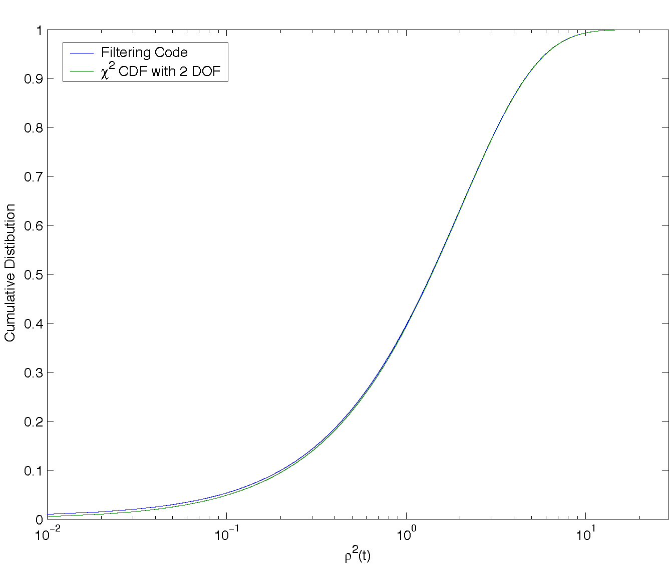
Figure 1: In the presence of Gaussian noise the expected filter output, $\rho^{2}(t)$, is the sum of the squares of two Gaussian distributed quantities and so should be $\chi^{2}$ distributed with two degrees of freedom. This figure shows the cumulative distribution function (CDF) of the filtering code output and the expected analytic value. The filter input is white Gaussian noise of variance $\varsigma^{2}$ and a constant power spectral density of $S_{n}\left(\left|f_{k}\right|\right)=2\varsigma^{2}\delta T$. It can be seen that there is good agreement between the observed and expected values.

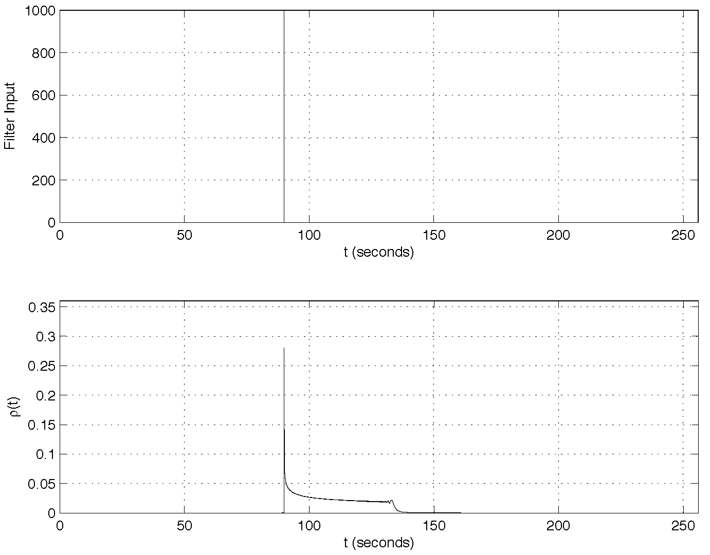
Figure 2: The top panel shows the filter input which consists of an impulse at $t_{0}=90$. The power spectrum is set to that of white uncorrelated noise. The bottom panel shows the output of the filter. The filter output is the sum of the squares of the time reverse chirps and the maximum of the filter output occurs at the time of the impulse.

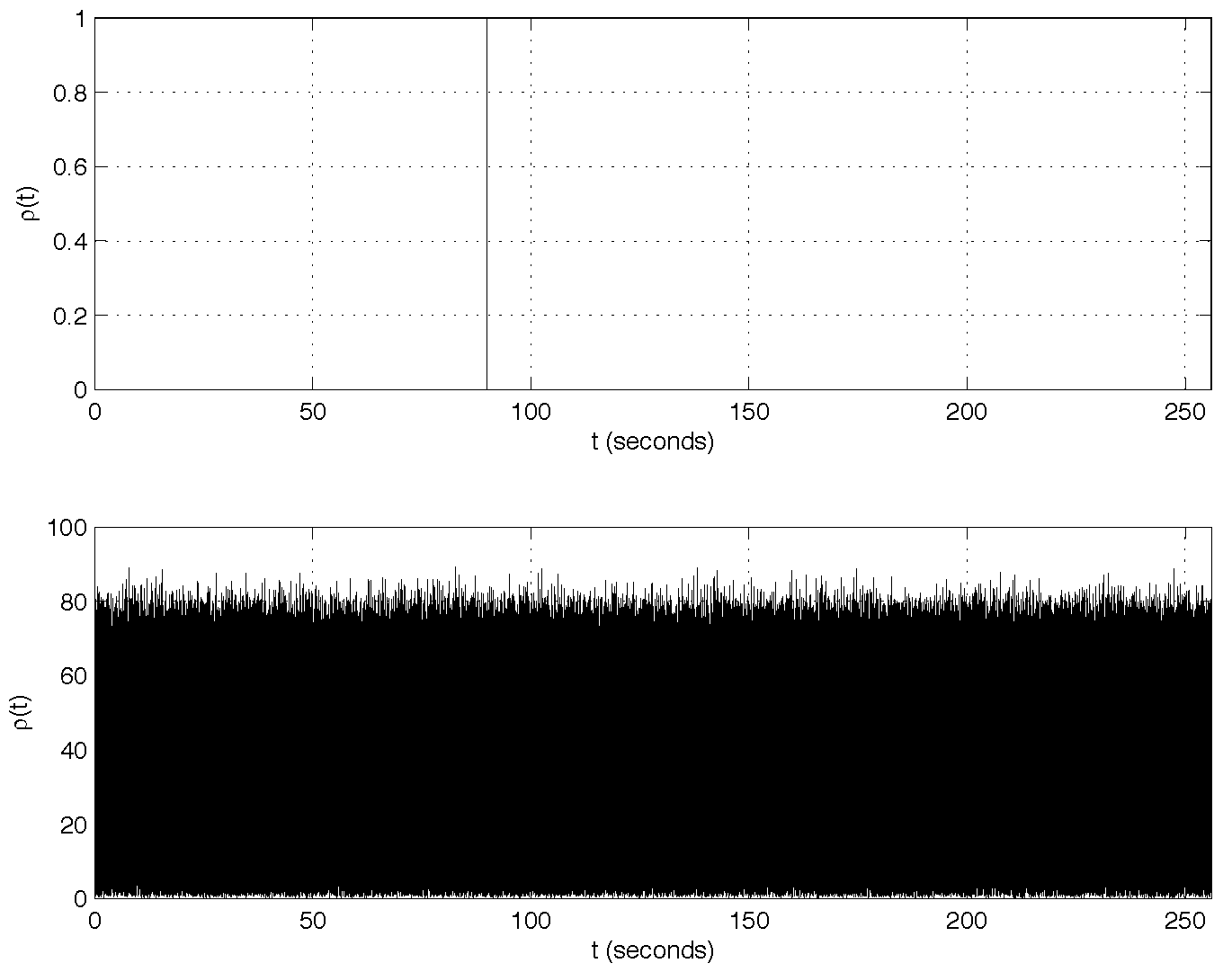
Figure 3: The top panel shows the filter input which consists of an impulse at $t_{0}=90$. The power spectrum is computed from Gaussian noise of the same length of the input data using Welch’s method. The bottom panel shows the output of the filter. Due to the fact that the duration of the inverse power spectrum $1/S_{n}\left(\left|f_{k}\right|\right)$ in the time domain is the same length as the data segment, the entire filter output is corrupted due to the wrap around of the FFT.

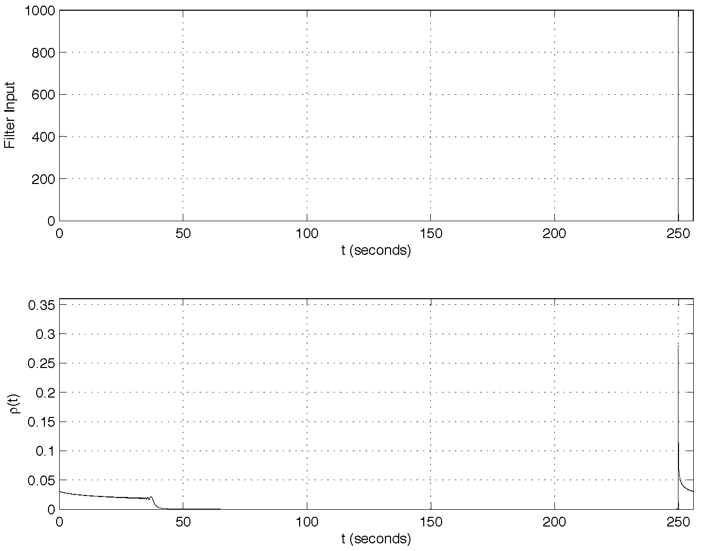
Figure 4: The top panel shows the filter input which consists of an impulse at $t_{0}=250$. The power spectrum is set to that of white uncorrelated noise. The bottom panel shows the output of the filter. The length of the chirp template is $43.7$ seconds. Notice that the filter output is non-zero for the first $37.7$ seconds of the output due to the wrap-around of the FFT.

Figure 5: In the presence of Gaussian noise the expected filter output, $\rho^{2}(t)$, is the sum of the squares of two Gaussian distributed quantities and so should be $\chi^{2}$ distributed with two degrees of freedom. This figure shows the cumulative distribution function (CDF) of the filtering code output and the expected analytic value. The filter input is white Gaussian noise of length $256$ seconds and the power spectrum $S_{n}\left(\left|f_{k}\right|\right)$ is computed from $15$ segments of white Gaussian noise length $256$ seconds, overlapped by $128$ seconds using Hann windowing and the median estimator.

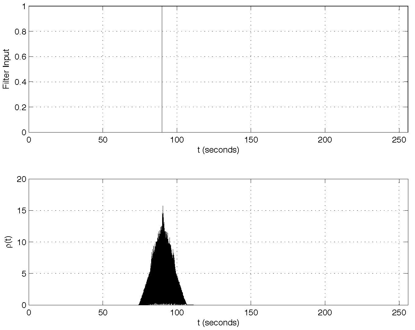
Figure 6: The top panel shows the input to the filtering code which is an impulse at $t=90$ seconds. The average power spectrum is computed from typical LIGO noise and then truncated to $16$ seconds in the time domain. The duration of non-zero filter output is also $16$ seconds.

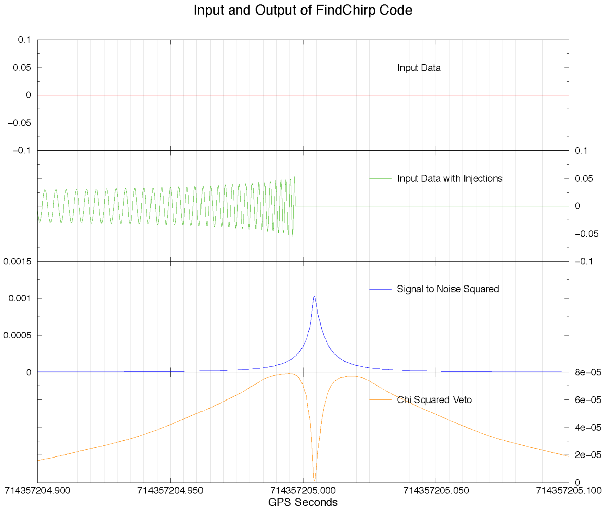
Figure 7: Output time series from the filtering code for an inspiral chirp in the absence of noise. A $(2.0,2.0)\,m_{\odot}$ inspiral chirp is generated using the post²-Newtonian time domain waveform generation and injected into the data. This is filtered using the post²-Newtonian stationary phase waveform. The signal to noise squared and $\chi^{2}$ time series are shown. The signal to noise squared is a maximum at the coalescence time of the template inspiral signal. This occurs slightly after the coalescence time of the injected signal. The difference in coalescence times is due to the different methods of generating the chirp signal.

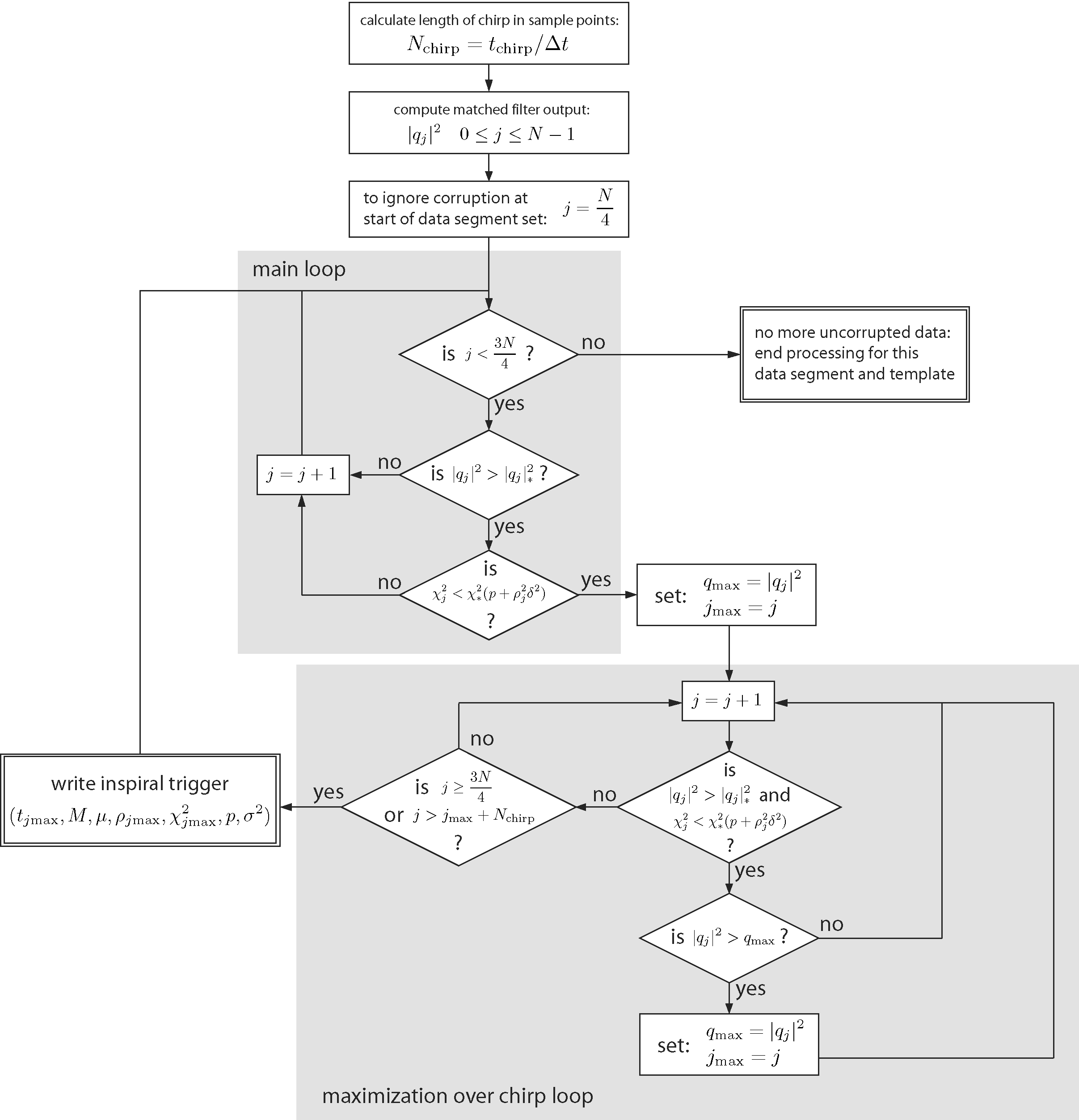
Figure 8: The algorithm used to generate inspiral triggers. For a given inspiral template we begin by calculating the length of the chirp and the filter output. For a data segment of length $N$, the first and last $N/4$ points in the segment may be corrupted due to FFT wrap-around, so we ignore them. For the rest of the data segment, we step through the filter output looking for times when the signal-to-noise and $\chi^{2}$ threshold are satisfied (the main loop). If we find a point that passes the threshold tests, we label it $j_{\mathrm{max}}$ and enter the maximization over chirp loop. This steps through the data looking for the any larger values of $|q_{j}|^{2}$ within a chirp length (given by $N_{\mathrm{chirp}}$) of the time $j_{\mathrm{max}}$. If a larger value of $|q_{j}|^{2}$ is found, we reset $j_{\mathrm{max}}$ and keep looking for any larger values. If no larger value is found within a chirp length (or we reach the end of the uncorrupted data) we generate an inspiral trigger and save its time, mass, signal-to-noise ratio, value of the $\chi^{2}$ veto, number of $\chi^{2}$ bin ($p$) and the value of $\sigma^{2}$ for this data segment.

Chapter 5 Detection Pipelines For Coalescing Binaries

Chapter 4 described the algorithms that we use to generate inspiral triggers given an inspiral template and a single data segment. There is more to searching for gravitational waves from binary inspiral than trigger generation, however. To perform a search for a given class of sources in a large quantity of interferometer data we construct a detection pipeline. In section 5.1 we give an overview of the the components used in a pipeline and how they fit together. We then describe the building blocks of the pipeline in more detail. Section 5.2 describes data quality cuts, which are used to discard data which is unsuitable for analysis. The application of trigger generation to the data is explained in section 5.3. The use of data from multiple interferometers is described in section 5.4. In section 5.5 we show how data from the interferometer that does not measure the gravitational wave signal can be used. Finally in section 5.8 we describe the pipeline that has been constructed to search for binary neutron stars and binary black hole MACHOs in the S2 data.

5.1 Construction of Inspiral Pipelines

A detection pipeline is a sequence of operations that starts with the raw data from the interferometers and produces a list of candidate events. Figure 1 shows a simple pipeline to filter the data from a pair of interferometers labeled IFO$1$ and IFO$2$. We only use data that comes from interferometers in stable operation. Running an interferometer is a complex process that requires human operators who are trained to lock the interferometers. Locking the interferometer is the process of bringing it from an uncontrolled state to a state where light is resonant in the interferometer. From a state in which the interferometer optics are freely swinging, the operators manually align the optics of the interferometer using the interferometer control systems. They then direct the automated lock acquisition system[Evans:thesis] to bring the Fabry-Perot cavities into resonance with the beam splitter positioned so that the light at the anti-symmetric port is a minimum. The recycling cavity is then brought into resonance and the length sensing and control servo maintains the locked state by monitoring the motion of the optics and adjusting their position accordingly. In addition to the operator, members of the LIGO Scientific Collaboration trained in the operation of the interferometer are present at the observatory. The collaboration member on duty is known as the as scientific monitor or scimon. Once the interferometer is locked, the operator and scimon decide if the quality of the data being recorded is suitable to be flagged as science mode data. If the data is suitable it passes the first cut for gravitational wave analysis and the operators and scimons continuously monitor the data using various data monitoring tools. Lock is lost when the length sensing servo no longer has enough dynamic range to maintain resonance in the interferometer. This is typically caused by large seismic events which may be local to the observatory (e.g. liquid nitrogen tanks creaking as the expand in the sun) or of global origin (e.g. a large earthquake in China has caused loss of lock). Poor data quality in the interferometer may also require a break in lock to remedy. Continuous locked operation has been maintained for up to $66.2$ hours in the Hanford 4km interferometer. Seismic noise in the Livingston interferometer limited the longest lock to $6.93$ hours during S2.

It is possible that the operators or scimons may make mistakes in deciding that data should be flagged as science mode; they may forget to enable calibration lines, for example. There may also be noise sources or transient events in the data which make it unsuitable for analysis but which are not easily detectable in the control room while the data is being taken. To prevent such data from being used in an astrophysical analysis a list of data quality cuts is compiled. The manual selection of science mode data may be considered the first data quality cut. Additional tests of data quality are described in section 5.2.

The chirp signals from compact binary inspiral depend on the masses and spins of the binary elements, as described in section 2.3. Searching for gravitational waves from BBHMACHOs requires signals which only depend on the masses $m_{1}$ and $m_{2}$ of the binary. The inspiral signals from BBHMACHOs lie in some region of the template parameter space described by the component masses $m_{1}$ and $m_{2}$. A single template is not sufficient to search for signals from the population, as the template for a given pair of mass parameters may not produce a high signal-to-noise ratio when used as a filter to detect a signal with different mass parameters. To search for signals from a region of parameter space we construct a bank of inspiral templates as described in section 5.3. The template bank is constructed to cover the parameter space in such a way that we do not discard any signals from our target population.

We then use the bank of templates to filter the data for inspiral signals using the matched filter and $\chi^{2}$ veto discussed in chapter 4. This results in a list of inspiral triggers. For the pipeline shown in figure 1, a bank of templates is generated used to filter the data for inspiral signals for each interferometer. We describe how trigger generation is used in a pipeline in section in detail in section 5.3.

One of the most powerful methods of rejecting false alarms is coincidence between different interferometers. As described previously, there are three LIGO interferometers which are operated simultaneously during science runs. The H1 and H2 detectors are co-located at the LIGO Hanford Observatory and the L1 detector is located at the LIGO Livingston Observatory. A true gravitational wave should produce a signal in all operating detectors at the same time, up to the time delay for the arrival of the wavefront of the gravitational wave at the observatories. We therefore require time coincidence, which demands that inspiral triggers be present in all operating detectors simultaneously, with time offsets less than the light travel time between detectors plus the measurement error of detection. While coincidence is the most obvious use of multiple interferometers, other coincidence tests may also be used, e.g. demanding consistency of the waveform parameters between the triggers from two detectors, or consistency in the recovered amplitude of the signal relative to the sensitivity of the detectors. We describe these tests in section 5.4.

While the goal during data acquisition is to ensure that the data recorded is as stationary and Gaussian as possible, transient noise artifacts may still be present in the data. For example, it has been seen that a person jumping up and down in the control room at the observatory will cause a burst of noise in the gravitational wave channel. There may also be occasional glitches in the interferometer control systems that cause a transient in the gravitational wave channel, despite the best efforts of the experimental team. To allow us to distinguish such events from true gravitational wave signals, we record several thousand data streams of auxiliary interferometer control channels and physical environment monitor (PEM) channels. Auxiliary channels monitor the state of the servo loops that control the interferometer and include information about the pre-stabilized laser, the length sensing and control system and the input and output optics. PEM channels record the data from devices such as seismometers, magnetometers and microphones placed in and around the interferometer. These devices are designed to detect environmental sources that may couple to signals in the gravitational wave channel. This data can be used to construct vetoes of the inspiral triggers if a coupling can be identified between a noise source present in an auxiliary or PEM channel and inspiral triggers in the gravitational wave channel. We demonstrate this process with examples in section 5.5.

The final step in constructing a pipeline is to turn the various elements described above (data quality cuts, template bank generation, trigger generation, coincidence and vetoing) into code that can be executed in an automated way on a computing cluster. The execution of the code must ensure that all the input data has been analyzed and the components of the pipeline are executed in the correct sequence. We use a directed acyclic graph (DAG) to describe the work flow of a pipeline. For example, we may construct construct a DAG to execute the simple pipeline in figure 1 on all the data from L1 and H1 recorded in S2. The DAG describing the work flow is submitted to a computing cluster via the Condor high throughput computing system[beowulfbook-condor]. The Condor DAG manager executes the pipeline described in the DAG that we generate. This process is described in more detail in section 5.8.3.

Implicit in the above discussion is that fact that there are many parameters that must be set at each stage of the pipeline. For example: What data quality cuts should we use? What signal-to-noise and $\chi^{2}$ thresholds should we use when generating the inspiral triggers? What coincidence tests should we apply and what should their parameters be? What auxiliary channels and PEM channels should be used as vetoes, and how do we apply these vetoes to inspiral triggers? Answering these questions is the key to turning a pipeline into a full binary inspiral search; we call the process of selecting the parameters tuning the pipeline. In fact, pipeline tuning and construction of the pipeline are not entirely separate. After constructing a pipeline and initial tuning, we may decide to revisit the pipeline topology before performing additional tuning.

When tuning the pipeline we may wish to minimize the false alarm rate, i.e. minimize the number of candidate events that are not due to inspiral signals. We may simultaneously wish to minimize the false dismissal rate to ensure that the pipeline does not discard triggers that are due to real signals. The false alarm rate can be studied by looking at candidate events in the playground. The false dismissal rate can be studied by injecting signals into the data, that is generating a known inspiral signal and adding it to the data before passing it through the pipeline. Injection of signals is described in section 5.7 and chapter 6.

When tuning the pipeline for data that will be used to produce an upper limit, we must ensure that we do not introduce statistical bias. A bias in the upper limit could be introduced, for example, by selecting PEM channel events to veto particular inspiral triggers which were associated with the PEM events purely by chance. Clearly this could systematically eliminate true inspiral events artificially in a way that would not be simulated in the efficiency measurements described below. To do avoid such a possibility, we select $10\%$ of all the data that we record as playground data. The data from GPS time $[t,t+600)$ is playground if

$$t-729273613\equiv 0\quad\mathrm{mod}(6370).$$ (5.1)

Playground data is selected algorithmically to provide a representative sample of the full data set. We are free to pursue whatever investigations we wish on the playground data. Although we do not use this data in the upper limit calculation, however we do not preclude the detection of a gravitational wave signal in this data. We describe the process of tuning the S2 binary black hole MACHO search in chapter 7.

If we are using data from multiple interferometers we can measure the background rate of inspiral signals. We do this by introducing a time shift into the data from different detectors before passing it through the pipeline. If we assume that noise between the detectors is uncorrelated and the time shift is sufficiently large, as described in section 5.6, then any candidate events that survive the pipeline should be due to noise alone and not astrophysical signals. By measuring the background rate, we can measure the false alarm rate of the pipeline which can be used for both tuning and the computation of the upper limit or detection confidence.

5.2 Data Quality Cuts

The theoretical matched filter is optimized for Gaussian data with a known, noise spectrum that is stationary over the time scale of the data analyzed. The filter therefore requires stable, well-characterized interferometer performance. In practice, the interferometer performance is influenced by optical alignment, servo control settings, and environmental conditions. The list of science mode data provided by the operators can contain times when the interferometer is not operating correctly. Unstable interferometer data can produce false triggers that may survive both the $\chi^{2}$ test and coincidence. Data quality cut algorithms evaluate the interferometer data over relatively long time intervals, using several different tests, or look for specific behavior in the interferometer to exclude science mode data that is unsuitable for analysis. To decide if we should exclude science mode data based on a particular data quality cut, we can examine the performance of the inspiral code on data which is flagged as suspect by the cut.

5.2.1 Photodiode Saturation

Figure 2 shows the signal-to-noise ratio and $\chi^{2}$ time series of the loudest candidate event that was produced by the LIGO S1 inspiral search[LIGOS1iul]. Also shown is the filter output for a simulated inspiral with similar parameters that was injected into well behaved interferometer data. Notice that the time series of $\rho(t)$, $\chi^{2}(t)$ and the raw data are very noisy around the time of the S1 loudest candidate. In contrast, the time series for the simulated signal is very clean. On further investigation, it was determined that the photodiode that records the light at the anti-symmetric port had saturated at the time of the S1 loudest event. The system that converts the light into an electronic signal for the length sensing and control servo had exceeded its dynamic range causing a noise transient in the data. The saturation is a symptom of poor interferometer performance. Photodiode saturations are caused by large bursts of noise in the gravitational wave channel which corrupt power spectral estimation and matched filtering. A test was developed to monitor the gravitational wave channel for photodiode saturations and this test has become a data quality cut for current and future searches.

5.2.2 Calibration Lines

A second example of a data quality cut is based on the presence of calibration lines, which were described in section 2.2.3. The calibration lines track the response of the instrument to mirror movement or a gravitational wave, which varies over time. Without the calibration lines, it is not possible to construct an accurate response function. Since the inspiral search needs correctly calibrated data, a simple data quality cut checks for the presence of the calibration lines in the data. If they are absent, the data is discarded.

5.2.3 Data Quality Cuts Available in S2

The full list of available data quality cuts and their meanings for S2 are show in Table 1. The table is divided into two sections, mandatory and discretionary data quality cuts. Mandatory cuts represent unrecoverable problems in data acquisition or calibration and so we must exclude these times from the list of science mode segments. Discretionary data cuts are optional for a particular search. For the inspiral search we decide whether or not to use a cut based on the performance of the trigger generation code in playground data when a particular data quality cut is active, as described in section 5.8.1. The times remaining after we apply data quality cuts are called science segments.

5.3 Inspiral Trigger Generation

Chapter 4 describes the algorithms that we use to determine if an inspiral from a binary of masses ${m_{1},m_{2}}$ is present in a single data segment. The input to trigger generation is:

1. The template, $\tilde{h}_{ck}$, drawn from a template bank.

2. The data segment to be filtered, $\{v_{j}\}$ $j\in[0,N]$, where $v_{j}$ is the raw (uncalibrated) interferometer output channel, LSC-AS_Q. A data segment is the unit of analysis for the filter and is a subset of a science segment.

3. An average power spectral density, $S_{v}(|f_{k}|)$, of the channel LSC-AS_Q,

4. The instrumental response function, $R(f_{k})$, which is required to calibrate the data and the power spectrum.

In this section, we describe how these quantities are constructed and used to generate inspiral triggers.

5.3.1 Template Banks

The matched filtering described in chapter 4 has been used to detect the inspiral waveforms from binary neutron stars in the mass range $1\,M_{\odot}\leq m_{1},m_{2}\leq 3\,M_{\odot}$ and binary black hole MACHOs in the mass range $0.2\,M_{\odot}\leq m_{2},m_{1}\leq 1\,M_{\odot}$. Since each mass pair $\{m_{1},m_{2}\}$ in the space produces a different waveform, we construct a template bank, a discrete subset of the continuous family of waveforms that belong to the parameter space. The placement of templates in the bank is determined by the mismatch of the bank, $\mathbb{M}$. The mismatch is the fractional loss in signal to noise that results when an inspiral signal, $s$, is not exactly correlated with a template in the bank, $h$. In terms of the inner product defined in equation 4.34 of section 4.1 it is

$$\mathbb{M}=1-\frac{(h|s)}{\sqrt{(h|h)(s|s)}}.$$ (5.2)

If we consider the distribution of binaries to be uniform in space, then the fraction of events lost due to the mismatch of the template from a population is approximately $\mathbb{M}^{3}$, i.e the range is decreased by a factor of $\mathbb{M}$. A mismatch of $3\%$, i.e. a $10\%$ loss of event rate, is conventionally accepted as a reasonable goal for binary neutron stars. For binary black hole MACHOs, we reduce the minimal match of the template bank to $5\%$. This is due to the fact that the number of templates in the bank for a given interferometer noise curve scales as approximately $m_{\mathrm{min}}^{-8/3}$, where $m_{\mathrm{min}}=m_{1}=m_{2}$ is the mass of the lowest mass equal mass template in the bank[Owen:1998dk]. If we lowering the minimal match then the computational cost decreases as $\mathbb{M}^{-1}$. The loss in signal-to-noise ratio is balanced by the fact that we are searching for a population of binary black hole MACHOs in the galactic halo. This population is far from homogeneous with almost all signals expected to produce a signal-to-noise ratio far above threshold, so this $5\%$ loss in signal-to-noise ration will hardly constitute any loss in observed event rate.

The scaling in the number of templates as a function of the lower mass of the bank parameter space is due to the fact that the number of templates required to achieve a given minimal match is a function of the number of cycles that the inspiral waveforms spends in the sensitive band of the interferometer. The more cycles the matched filter correlates against, the greater its discriminating power and so the loss in signal-to-noise ratio for a mismatched template increases. A pair of inspiralling $1.4\,M_{\odot}$ neutron stars have $347$ cycles in the S2 sensitive band (between $100$ Hz and $2048$ Hz), compared to $1960$ cycles for a pair of $0.5\,M_{\odot}$ binary black hole MACHOs; a pair of $0.1\,M_{\odot}$ binary black hole MACHOs have nearly $28\,500$ cycles.

Since the number of templates is a function of the number of cycles of an inspiral in the sensitive band of the interferometer, it also depends on the shape of the power spectral density of the noise curve. In fact location of the templates in the bank is also a function of the PSD, as described in [Owen:1998dk]. The power spectrum of the instrument changes over time and so we must also change the template bank. We accomplish this by using the power spectral density for an analysis chunk to generate a template bank that is unique to that chunk. The PSD is calibrated and the template bank generated. Figure 5 shows binary neutron star and binary black hole MACHO template banks generated for a typical stretch of S2 data. The smallest and largest number of templates in a bank during S2 was $589$ and $857$ binary neutron star templates and $11\,588$ and $17\,335$ binary black hole MACHO templates.

5.3.2 Data Management

Corruption due to the wrap-around of the matched filter means that not all the time in a data segment can be searched for triggers. As described in chapter 4, we simplify the process of selecting uncorrupted data by only searching for triggers in the signal-to-noise ratio, $\rho^{2}(t_{j})$, when

$$\frac{N}{4}\leq j<\frac{3N}{4},$$ (5.3)

where $N$ is the number of sample points in the data segment, and by demanding that the amount of data corrupted is less than $N/4$ sample points. To ensure that all data is analyzed we must overlap each data segment by $(N/2)\Delta t$ seconds. To compute an average power spectrum we require a sample of data near the data segment being filtered so that a good estimate of the noise can be obtained. We combine these two requirements by bundling several overlapping data segments together in an analysis chunk. The length of an analysis chunk is bounded above by the amount of memory available in the computers performing the filtering and bounded below by requiring a sufficiently large number of segments in the computation of the average power spectrum. In the S2 pipeline, we construct analysis chunks of length $2048$ seconds from $15$ overlapped data segments of length $256$ seconds. The data segments are overlapped by $128$ seconds, with the first and last $64$ seconds of data segment ignored when searching for triggers. The analysis chunks themselves are overlapped by $128$ seconds so that only the first and last $64$ seconds of a science segment are not searched for inspiral triggers.

Figure 4 shows how analysis chunks are constructed from the science segments in S2. The first analysis chunk is aligned with the start of the science segment. Subsequent chunks overlap the previous one by $128$ seconds. At the end of a science segment there is generally not enough data to fit an entire analysis chunk but we cannot make the chunk shorter, as we need all $15$ data segments to compute the average power spectrum. To solve this problem, we align the end of the last chunk with the end of the science segment and ignore any inspiral triggers generated for times that overlap the previous chunk.

The interferometer records data at $16\,384$ Hz, and we down sample the analysis chunk after reading it from disk to decrease the computational resources required by the filtering code. We choose the new sample rate so that the loss in signal-to-noise ratio due to the discrete time steps, $\Delta t$, is less than that due to the discrete choices of the template mass parameters. It can be shown that for the initial LIGO noise curve, this is true if the sample rate of the filtered data is greater than $\sim 2600$ Hz[Owen:1998dk]. For simplicity, we chose sample rates that are powers of two and so we resample the data to $4096$ Hz. We do this by applying a finite impulse response (FIR) low pass filter to remove power above the Nyquist frequency of the desired sample rate, $2048$ Hz. The low passed data is then decimated to the desired sample rate. Although the maximum frequency of most of the BBHMACHO inspiral signals is greater than $2048$ Hz, the loss of signal-to-noise ratio above this frequency is negligible as most of the the signal-to-noise is accumulated at frequencies lower than $2048$ Hz, as described in chapter 2. Figure 3 shows the loss in signal-to-noise ratio of a BBHMACHO inspiral due to resampling. The inspiral waveform of a pair of $0.2\,M_{\odot}$ black holes an effective distance of $25$ kpc is generated at a sample rate of $16\,384$ Hz. The maximum frequency of this waveform is $10\,112$ Hz. The waveform is injected into raw (un-resampled) data with a typical S2 noise curve which is then filtered at $16\,384$ Hz and $4096$ Hz. The maximum of the signal-to-noise ratio is $\rho=73.67$ for the raw data and $\rho=73.58$ for the resampled data, giving a difference in signal-to-noise ratio of $0.1\%$. This loss combines the effects due to the discreteness of the resampled data and the signal present above the Nyquist and is much less than the $5\%$ loss in signal-to-noise ratio caused by the discrete nature of the template bank.

The interferometer data contains a large amount of power of seismic origin at low frequencies. This power is several orders of magnitude higher than the noise in the sensitive frequency band of the interferometer. This power may bleed across the frequency band when the data is Fourier transformed into the frequency domain and dominate the true noise in the sensitive band of the interferometer, In order to prevent this, we apply a Butterworth infinite impulse response (IIR) high pass filter to the resampled data. The high pass frequency and filter order are chosen so that power in the sensitive band of the interferometer is not attenuated. The data is filtered forwards and backwards through the filter to remove the dispersion of the filter. The data used to compute the power spectral estimate is windowed using a Hann window to prevent power from line features in the spectrum (e.g. power line harmonics or suspension wire resonances) from bleeding into adjacent frequency bands. We also apply a low frequency cutoff in the frequency domain at a slightly higher frequency than the time domain filter. The matched filter correlation is not computed below this cutoff, so frequencies below it do not contribute to the signal-to-noise ratio.

A windowed copy of each of the $15$ data segment is used to construct the average power spectral density used in the matched filter, as described in section 4.6. Note that the data used in the matched filter is not windowed; the windowed data is discarded once it has been used to compute the power spectra. The mean values over the analysis chunk of the calibration parameters $\alpha$ and $\beta$ are used to construct the response $R(f_{k})$, as described in equation (2.62) of section 2.2.3. The same response function is used to calibrate the power spectral density and all data segments in the chunk.

A disadvantage to the above method of processing the input data is that we require a science segment to be at least $2048$ seconds long. Any shorter science segments are ignored, as there is not enough data to generate a power spectral density. We note here that this lead to a significant amount of data being discarded in the S2 analysis. As we will describe below, the S2 pipeline requires the L1 interferometer to be operating in order to analyze the data. L1 is the least stable of the interferometers as it is very sensitive to seismic noise. High seismic noise can saturate the length sensing and control servo and cause the loss of lock, which terminates a science segment. Modification of the data management (e.g. construction of analysis chunks and power spectral estimation) to allow us to use science segments shorter than $2048$ seconds requires significant changes of the implementation of the inspiral search code. It was not possible to implement and test these changes within the time allowed to perform the S2 analysis. Fortunately, it is expected that after the installation of addition seismic isolation at the Livingston observatory, scheduled for completion in late 2004, the lengths of science segments will be significantly increased and the number of short segments discarded will decrease. Unfortunately data from the third science run, S3, which was completed before the seismic upgrade, exhibits the problem of short science segments, so a redesign of the filtering code may still be required.

5.3.3 Trigger Generation Parameters

The process of template bank construction and inspiral trigger generation relies on several parameters that can be tuned to minimize the false dismissal or false alarm rate. We have touched on some of these already; in this section we enumerate all of the tunable parameters for bank and inspiral trigger generation.

Both template bank and inspiral trigger generation require a calibrated power spectral density. In the inspiral trigger generation described above, construction of the PSD is coupled to the length of the data segments and analysis chunks. The following data conditioning parameters are used to construct the data segments, and so determine the characteristics of the PSD:

• Number of sample points in a data segment, $N$. This determines the length of the segments correlated in the matched filter and the length of the segments used in the PSD estimate. The number of points that subsequent data segments are overlapped by is then $N_{\mathrm{overlap}}=N/2$.

• Number of data segments in a chunk $N_{\mathrm{segments}}$. This sets the number of data segments used in the PSD estimate and so the number of segments in an analysis chunk.

• Sample Rate, $1/\Delta t$. The sample rates used in LIGO data analysis are integer powers of two Hertz.

• Number of non-zero points in the square root of inverse power spectrum in the time domain, $N_{\mathrm{invspectrunc}}$. This parameter was described in detail in section 4.7.

We set $\Delta t\,N_{\mathrm{invspectrunc}}=16$ seconds for the S2 analysis based on the length of wraparound corruption allowed. A systematic study of the value of $N_{\mathrm{invspectrunc}}$ has not been carried out for the S1 or S2 data, but is planned for future analysis.

Once the above parameters have be specified, it follows that the number of sample points in an analysis chunk is

$$N_{\mathrm{chunk}}=\left(N_{\mathrm{segments}}-1\right)N_{\mathrm{stride}}+N$$ (5.4)

where

$$N_{\mathrm{stride}}=N-N_{\mathrm{overlap}}.$$ (5.5)

The length of the analysis chunk, in seconds, is therefore

$$T_{\mathrm{chunk}}=\Delta t\,N_{\mathrm{chunk}}.$$ (5.6)

The choice of these parameters is governed by the class of waveforms searched for and the low frequency sensitivity of the interferometer. The longest inspiral waveform in the template bank (which will be the smallest mass template), is determined by the lowest sensitive frequency of the interferometer. The sum of the length of the longest template and the length of the inverse power spectrum must be shorter than the duration of the signal-to-noise output, $\rho(t)$, that we ignore due to corruption. We therefore require

$$\frac{1}{4}N\geq 2N_{\mathrm{invspectrunc}}+N_{\mathrm{longest}}$$ (5.7)

where $N_{\mathrm{longest}}$ is the number of points in the longest chirp.

Other data conditioning parameters control the cut-offs of the time and frequency domain filters applied to the data. These are:

• The high pass filter cutoff, $f_{\mathrm{hp}}$, and high pass filter order $O_{\mathrm{hp}}$. These parameters determine the shape of the IIR Butterworth high pass filter applied to the analysis chunks before PSD estimation and inspiral trigger generation.

• The frequency domain low frequency cut off, $f_{\mathrm{low}}$. This parameter allows us to exclude frequencies below a certain value from the correlations in the matched filter and $\chi^{2}$ veto. A non-zero value of $f_{\mathrm{low}}$ sets the value of the data in all frequency bins $k<k_{\mathrm{min}}=f_{\mathrm{low}}/(N\Delta t)$ to zero which excludes this data from the correlation. Note that $f_{\mathrm{low}}\geq f_{\mathrm{hp}}$ to prevent data used in the correlation being attenuated by the high pass filter.

During investigation of inspiral triggers in the S2 playground data, it was discovered that many of the L1 inspiral triggers appeared to be the result of non-stationary noise with frequency content around $70$ Hz. An important auxiliary channel, L1:LSC-POB_I, proportional to the residual length of the power recycling cavity, was found to have highly variable noise at $70$ Hz. There are understandable physical reasons for this, namely the power recycling servo loop (for which L1:LSC-POB_I is the error signal) has a known instability around $70$ Hz, which often results in the appearance of glitches in the detector output channel at around $70$ Hz. As a consequence, it was decided that to reduce sensitivity to these glitches the high pass cut off should be set to $f_{\mathrm{hp}}=100$ Hz with order $O_{\mathrm{hp}}=8$ and the low-frequency cutoff set to $f_{\mathrm{low}}=100$ Hz. This subsequently reduced the number of inspiral triggers (presumably created by this problem); an inspection of artificial signals injected into the interferometer revealed a very small loss of efficiency for binary neutron star inspiral and BBHMACHO signal detection resulting from the increase in the low frequency cutoff.

After we have defined the data conditioning parameters and a parameter space for the search, the only remaining free parameter for template bank generation is:

• The template bank mismatch, $\mathbb{M}\in[0,1)$. Given a value of mismatch, $\mathbb{M}$, for a real signal that lies in the bank parameter space the fractional loss in signal-to-noise ration should be no larger than $\mathbb{M}$ when filtering with the signal against its exact waveform compared to filtering the signal against the template in the bank with yields the highest signal-to-noise ratio.

As described above, the value chosen for the S2 search is $\mathbb{M}_{\mathrm{BBHMACHO}}=5\%$. Note that we do not truncate the power spectrum used for generating the template bank, as there is no issue with wrap-around in the bank generation algorithm.

For a given template we use matched filtering to construct the signal-to-noise ratio, $\rho$, and search for times when this exceeds a threshold, $\rho>\rho^{\ast}$. If the threshold $\rho_{\ast}$ is exceeded, we construct the template based veto, $\chi^{2}$, with $p$ bins. Small values of $\chi^{2}$ indicate that the signal-to-noise was accumulated in a manner consistent with an inspiral signal. If the value of the $\chi^{2}$ veto is below a threshold, $\chi^{2}<\chi^{2}_{\ast}(p+\delta^{2}\rho^{2})$, then an inspiral trigger is recorded at the maximum value of $\{\rho|\chi^{2}<\chi^{2}_{\ast}(p+\delta^{2}\rho^{2})\}$. The parameters used available in trigger generation are:

• The signal to noise threshold, $\rho_{\ast}$.

• The $\chi^{2}$ threshold, $\chi^{2}$.

• The number of bins used in the $\chi^{2}$ veto, $p$.

• The parameter $\delta^{2}$ used to account for this mismatch of a signal and template in the $\chi^{2}$ veto, as described in section 4.8.2.

Tuning of these trigger generation parameters is particular to the class of search used. A detailed discussion of this tuning is for binary black hole MACHOs is given in chapter 7.

5.4 Trigger Coincidence

Coincidence is a powerful tool for reducing the number of false event candidates surviving a pipeline. The simplest test of coincidence is time coincidence of triggers between two or more interferometers. For a trigger to be considered coincident in two interferometers, we demand that it is observed in both interferometers within a temporal coincidence window $\delta t$. The coincidence window must allow for the error in measurement of the time of the trigger. It must also allow for the difference in gravitational time of arrival if the interferometers are not located at the same observatory. The time difference between gravitational wave arrival time varies from $0$ seconds, if the gravitational wave is propagating perpendicular to a line joining the detectors, to $10$ ms if the gravitational wave is propagating parallel to a line joining the detectors. The maximum time difference comes from the time it takes a gravitational wave to propagate between the observatories, given by $t=\frac{d}{c}$, where $d=3002$ km is the distance between the observatories and $c$ is the speed of light (the propagation speed of gravitational waves). Monte Carlo analysis with simulated signals suggests that we cannot measure the time of the trigger to an accuracy of less than $1$ ms. The time coincidence window is therefore $\delta t=1$ ms if the interferometers are located at the same observatory. For coincidences between LHO and LLO triggers, we set $\delta t=3000\,\mathrm{km}/c+1\,\mathrm{ms}=11\,\mathrm{ms}$. Any triggers that fail this test are discarded.

If a signal found in temporal coincidence is generated by real inspiral, it should have the same waveform in both interferometers, up to issues of the different detector antenna patterns yielding different combinations of $h_{+}$ and $h_{\times}$. This suggests that we could apply a waveform parameter test to triggers candidate that survive the time coincidence test. We cannot exactly extract the parameters of the waveform, however, since we filter the interferometer data with a template bank which may not contain the true waveform. In addition to this, the template banks will, in general, differ between detectors and detector noise may cause error in the measurement of the signal parameters, even if the template banks are the same. To account for these sources of error, we can apply waveform parameter coincidence by requiring that the two mass $m_{1}$ and $m_{2}$, of the templates are identical to within an error of $\delta m$.

We now consider an amplitude cut on the signals. The Livingston and Hanford detectors are not co-aligned. There is a slight misalignment of the detectors due to the curvature of the earth and so the antenna patterns of the detectors differ. This causes the measured amplitude and phase of a gravitational wave to differ between the sites. In the extreme case, it is possible, for example, for a binary to be completely undetectable by the L1 detector, but still detectable by the H1 and H2 detectors. For a given inspiral trigger, we measure the effective distance of the binary system. This is the distance at which an optimally oriented binary would produce the observed signal-to-noise ratio in a particular instrument—it is not the true distance of the binary. Since the detectors have different antenna patterns they will report different effective distances for the same gravitational wave. Figure 6 shows the ratio of effective distances between the two LIGO observatories for the population of binary neutron stars considered in the S2 analysis. The significant variation of the ratio of the effective distances precludes using a naive test for amplitude coincidence. It is possible to obtain information about sky position from time delay between sites to construct a more complicated amplitude cut, but this has not be used in the S2 analysis.

In the case of triggers from the H1 and H2 interferometers that are coincident in time and mass, we can apply an amplitude cut that tests that the effective distances of the triggers are coincident. In this test we must allow for the relative sensitivity of the detectors while allowing for error in the distance measurement, as determined by Monte Carlo simulations. The amplitude cut for triggers from H1 and H2 is given by

$$\frac{\left|\mathcal{D}_{\mathrm{1}}-\mathcal{D}_{\mathrm{2}}\right|}{D_{\mathrm{1}}}<\frac{\epsilon}{\rho_{\mathrm{2}}}+\kappa,$$ (5.8)

where $\mathcal{D}_{1}$ ($\mathcal{D}_{2}$) is the effective distance of the trigger in the first (second) detector and $\rho_{2}$ is the signal-to-noise ratio of the trigger in the second detector. $\epsilon$ and $\kappa$ are tunable parameters. In order to disable the amplitude cut when comparing triggers from LLO and LHO, we set $\kappa=1000$. When testing for triple coincident triggers we accept triggers that are coincident in the L1 and H1 detectors that are not present in the H2 detector if the effective distance of the trigger is further than the maximum distance of H2 at the signal-to-noise ratio threshold at the time of the candidate trigger. Figure 7 summarizes the algorithm for the time, mass and distance coincidence tests used in S2.

We therefore have the following coincidence parameters that must be tuned for the pipeline:

• The time coincidence window, $\delta t$, which is set to $1$ ms for LHO-LHO coincidence and $11$ ms for LHO-LLO coincidence.

• The mass coincidence window, $\delta m$.

• The error on the measured effective distance due to the instrumental noise, $\epsilon$, in the amplitude test.

• The systematic error in measured effective distance, $\kappa$, in the amplitude test.

If coincident triggers are found in H1 and H2, we can get an improved estimate of the amplitude of the signal arriving at the Hanford site by coherently combining the filter outputs from the two gravitational wave channels,

$$\rho_{H}=\sqrt{\frac{|z_{H1}+z_{H2}|^{2}}{\sigma_{H1}^{2}+\sigma_{H2}^{2}}},$$ (5.9)

where $z$ is the matched filter output given by equation (4.88). In this combination, the more sensitive interferometer receives more weight in the combined signal-to-noise ratio. If a trigger is found in only one of the Hanford interferometers, then $\rho_{H}$ is simply taken to be the $\rho$ from that interferometer.

Finally, we cluster the coincident triggers over a $4$ second time interval. Clustering is performed so that a noise transient that may cause several templates to trigger within a small window is only counted as a single event in the data sample.

5.5 Auxiliary and Environmental Channel Vetoes

In addition to data quality cuts, another method to exclude false alarms is to look for signatures in environmental monitoring channels and auxiliary interferometer channels which would indicate an external disturbance or instrumental glitches. This allows us to veto any triggers recorded at that time. Auxiliary interferometer channels (which monitor the light in the interferometer at points other than the antisymmetric port—where a gravitational wave would be most evident) are examined, with the aim being to look for correlations between glitches found in the readouts of these channels and inspiral event triggers found in the playground data. By doing so, we are capable of identifying instrumental artifacts that directly affect the light that is measured in the gravitational wave channel, so these vetoes are potentially very powerful. Figure 8 demonstrates the the use of auxiliary channels to identify the source of an inspiral trigger in the gravity wave channel.

When choosing vetoes, we must consider the possibility that a gravitational wave itself could produce the observed glitches in the auxiliary channel due to some physical or electronic coupling. This possibility was tested by means of hardware injections, in which a simulated inspiral signal is injected into the interferometer by physically moving one of the end mirrors of the interferometer. Hardware injections allow us to establish a limit on the effect that a true signal would have on the auxiliary channels. Only those channels that were unaffected by the hardware injections were considered “safe” for use as potential veto channels. The process of testing veto safety with hardware injections is described in more detail in chapter 6.

We used a computer program, glitchMon[glitchMon], to examine the data and identify large amplitude transient signals in auxiliary channels. Numerous channels, with various filters and threshold settings, were examined and which produced a list of times when the glitches occurred. The glitch event list was compared with times generated by triggers from the inspiral search (Note that these studies were all conducted on the playground data.) A time window around a glitch was defined, and any inspiral event within this window was rejected. One can associate the veto with inspiral event candidates and evaluate a veto efficiency (percentage of inspiral events eliminated), use percentage (percentage of veto triggers which veto at least one inspiral event), and dead-time (percentage of science-data time eliminated by the veto). A “good” veto will have a large veto efficiency and use percentage with a small dead time suggesting that it is well correlated with events in the gravitational wave channel that produce inspiral triggers. Followup studies are performed on such candidate vetoes to determine the physical coupling between the auxiliary channel and the gravitational wave channel. If a sound coupling mechanism is found, then the veto will be used.

Tuning of the vetoes for binary black hole MACHOs is described in chapter 7.

5.6 Background Estimation

Since we restrict the S2 analysis to coincident data and require that at least two of the interferometers must be located at different observatories, we may measure a background rate for our analysis. We estimate the background rate by introducing an artificial time offset, or lag, $\mathbb{T}$ to the triggers coming from the Livingston detector relative to the Hanford detector. We call this “sliding the triggers by $\mathbb{T}$.” After generating triggers for each interferometer, we slide the triggers from the LHO interferometers relative to the LLO interferometer and look for coincidences between the offset and zero lag triggers. The triggers which emerge from the end of the pipeline are then considered a single trial representative of an output from a search if no signals are present in the data. By choosing a lag of more than 20 ms, we ensure that a true gravitational wave will not be coincident in the time-shifted data streams. In fact, we use lags longer than this to avoid correlation issues; the minimum lag is $17$ seconds. Note that we do not time-shift the two Hanford detectors relative to one another since there may be real correlations due to environmental disturbances. If the times of background triggers are not correlated in the two interferometers then the background rate can be measured; we assume that there is no such correlation between LHO and LLO triggers.

5.7 Detection Efficiency

In absence of detection, we will construct an upper limit on event rate. To do this we need to measure the detection efficiency, $\varepsilon$, of the analysis pipeline to our population. This is the fraction of true signals from a population that would produce triggers at the end of the pipeline. A Monte Carlo method is used to measure this efficiency. We simulate a population of binary neutron stars and inject signals from that population into the data from all three LIGO interferometers. The injection is performed in software by generating an inspiral waveform and adding it to interferometer data immediately after the raw data is read from disk. We inject the actual waveform that would be detected in a given interferometer accounting for both the masses, orientation, polarization, sky position and distance of the binary, the antenna pattern and calibration of the interferometer into which this signal is injected. The effectiveness of software injections for measuring the response of the instrument to an inspiral signal is validated against hardware injections where an inspiral signal is added to the interferometer control servo during operation to produce the same output signal as a real gravitational wave. This validation is described in chapter 6. The data with injections is run through the full analysis pipeline to produce a list of inspiral triggers. We may combine the signal-to-noise rations from coincident triggers from several interferometers into a single coherent signal-to-noise ratio,

$$\hat{\rho}=f(\rho_{\mathrm{L1}},\rho_{\mathrm{H}})$$ (5.10)

where the form of $f$ is chosen based on studies of the playground and background triggers. We can then construct a final threshold, $\hat{\rho}_{\ast}$, on triggers that survive the pipeline. The detection efficiency, $\varepsilon(\hat{\rho})$, is the ratio of the number of signals with $\hat{\rho}>\hat{\rho}_{\ast}$ to the number of injected signals.

5.8 The S2 Data Analysis Pipeline

In this section we describe the pipeline constructed to search the S2 data for gravitational waves from inspiralling binary neutron stars and binary black hole MACHOs. The data quality cuts used are common to both searches and are described in section 5.8.1. The detection of a gravitational-wave inspiral signal in the S2 data would (at the least) require triggers in both L1 and one or more of the Hanford instruments with consistent arrival times (separated by less than the light travel time between the detectors) and waveform parameters. During the S2 run, the three LIGO detectors had substantially different sensitivities, as can be seen from figure 9. The sensitivity of the L1 detector was greater than those of the Hanford detectors throughout the run. Since the orientations of the LIGO interferometers are similar, we expect that signals of astrophysical origin detected in the Hanford interferometers will most often be also detectable in the L1 interferometer. We use this and the requirement that a signal be detected in both the Livingston and at least one of the Hanford interferometers to construct a triggered search pipeline.

5.8.1 Selection of Data Quality Cuts for S2

Playground data from each of the three interferometers was analyzed separately producing a list of inspiral triggers from each interferometer. Only the mandatory data quality cuts were used to exclude time from the science mode segments. Each interferometer was filtered separately using template banks particular to that interferometer. No coincidence was applied between interferometers; data quality cuts were tested independently on the three lists of inspiral triggers produced. Table 2 shows the the correlation of inspiral triggers with a particular data quality cut for triggers of different signal to noise. When selecting the data quality cuts we must be aware of three constraints. The first is that the data quality cuts are based on data from the gravitational wave channel so it is important to ensure that a data quality cut is not triggered by a real signal in the data. For this reason we always use caution when selecting a cut base on noise in AS_Q. The second constraint is that we do not wish to exclude large amounts of data from the analysis. Finally we base our choice on advice from the experimental team. A member of the experimental team may decide that a cut should be used, even if it does not correlate with inspiral triggers, as any detection made in such a time could not be trusted. Table 3 shows the final choice of discretionary data quality cuts and the reasons for them.

5.8.2 A triggered search pipeline

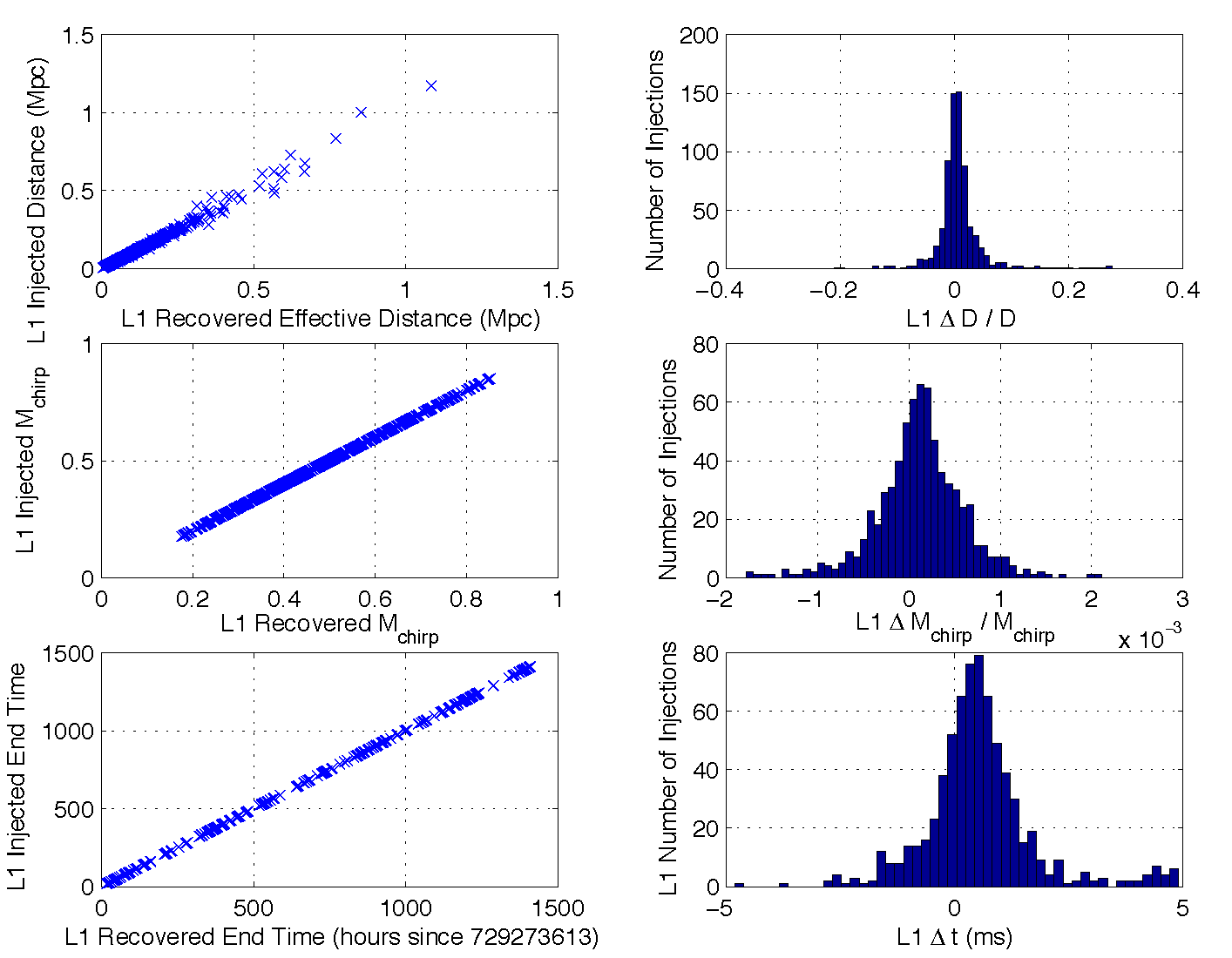
Figure 10: The panels in this figure compare the measured values of effective distance, chirp mass and end time with the known values for the injected waveforms in the Monte Carlo simulation in the L1 detector.

During the S2 run, the three LIGO detectors had substantially different sensitivities, as can be seen from figure 9. The Livingston interferometer is more sensitive than either of the Hanford interferometers. We use this and the requirement that a signal be detected in both the Livingston and at least one of the Hanford interferometers to construct a triggered search pipeline, summarized in Fig. 10. We search for inspiral triggers in the most sensitive interferometer (L1), and only when a trigger is found in this interferometer do we search for a coincident trigger in the less sensitive interferometers. This approach reduces the computational power necessary to perform the search.

The power spectral density (PSD) of the noise in the Livingston detector is estimated independently for each L1 chunk that is coincident with operation of a Hanford detector (denoted $\mathrm{L1}\cap(\mathrm{H1}\cup\mathrm{H2})$). The PSD is used to lay out a template bank for filtering that chunk, according to the parameters for mass ranges and minimal match[Owen:1998dk]. The data from the L1 interferometer for the chunk is then filtered, using that bank, with a signal-to-noise threshold $\rho_{\mathrm{L}}^{\ast}$ and $\chi^{2}$ veto threshold $\chi^{2}_{\ast\mathrm{L}}$ to produce a list of triggers as described in section 5.3. For each chunk in the Hanford interferometers, a triggered bank is created by adding a template if it produced at least one trigger in L1 during the time of the Hanford chunk. This is used to filter the data from the Hanford interferometers with signal-to-noise and $\chi^{2}$ thresholds specific to the interferometer, giving a total of six thresholds that may be tuned. For times when only the H2 interferometer is operating in coincidence with L1 (denoted $\mathrm{L1}\cap(\mathrm{H2}-\mathrm{H1})$) the triggered bank is used to filter the H2 chunks that overlap with L1 data; these triggers are used to test for L1-H2 double coincidence. All H1 data that overlaps with L1 data (denoted $\mathrm{L1}\cap\mathrm{H1}$) is filtered using the triggered bank for that chunk. For H1 triggers produced during times when all three interferometers are operating, a second triggered bank is produced for each H2 chunk by adding a template if it produced at least one trigger found in coincidence in L1 and H1 during the time of the H2 chunk and the H2 chunk is filtered with this bank. These triggers are used to search for triple coincident triggers in H2. The remaining triggers from H1 when H2 is not available are used to search for L1-H1 double coincident triggers.

5.8.3 A directed acyclic graph (DAG) for the S2 pipeline

In this section we demonstrate how the S2 pipeline in figure 10 can be abstracted into a DAG to execute the analysis. We illustrate the construction of the DAG with the short list of science segments shown in table 4. For simplicity, we only describe the construction of the DAG for zero time lag data. The DAG we construct filters more than the absolute minimum amount of data needed to cover all the double and triple coincident data, but since we were not computationally limited during S2, we chose simplicity over the maximum amount of optimization that could have used.

A DAG consists of nodes and edges. The nodes are the programs which are executed to perform the inspiral search pipeline. In the S2 pipeline, the possible nodes of the DAG are:

1. datafind locates data for a specified time interval on the compute cluster and creates a file containing the paths to the input data that other programs can read.

2. tmpltbank generates an average power spectral density for a chunk and computes a template bank for a given region of mass parameter space and minimal match.

3. inspiral filters an analysis chunk using a template bank and generates inspiral triggers for further analysis.

4. trigtotmplt generated a triggered template bank from the output of the inspiral code.

5. inca (INspiral Coincidence Analysis) implements the coincidence analysis described in section 5.4 and figure 7.

The edges in the DAG define the relations between programs; these relations are determined in terms of parents and children, hence the directed nature of the DAG. A node in the DAG will not be executed until all of its parents have been successfully executed. There is no limit to the number of parents a node can have; it may be zero or many. In order for the DAG to be acyclic, no node can be a child of any node that depends on the execution of that node. By definition, there must be at least one node in the DAG with no parents. This node is executed first, followed by any other nodes who have no parents or whose parents have previously executed. The construction of a DAG allows us to ensure that inspiral triggers for two interferometers have been generated before looking for coincidence between the triggers, for example.

The S2 DAG is generated by a program called the pipeline script, which is an implementation of the logic of the S2 pipeline in the Python programming language. The pipeline script takes as input the list of science segments for each interferometer, with data quality cuts applied. The script reads in all science segments longer than $2048$ seconds and divides them into master analysis chunks. If there is data at the end of a science segment that is shorter than $2048$ seconds, the chunk is overlapped with the previous one, so that the chunk ends at the end of the science segment. An option named trig-start-time is set and passed to the inspiral code. No triggers are generated before this time and so no triggers are duplicated between chunks. For example, the first L1 science segment in the fake segment list in table 4 starts at GPS time 730000000 and ends at GPS time 730010000. It is divided into the following master chunks:

<AnalysisChunk: start 730000000, end 730002048>
<AnalysisChunk: start 730001920, end 730003968>
<AnalysisChunk: start 730003840, end 730005888>
<AnalysisChunk: start 730005760, end 730007808>
<AnalysisChunk: start 730007680, end 730009728>
<AnalysisChunk: start 730007952, end 730010000, trig_start 730009664>

Although the script generates all the master chunks for a given interferometer, not all of them will be filtered. Only those that overlap with double or triple coincident data are used for analysis. The master analysis chunks are constructed for L1, H1 and H2 separately by reading in the three science segment files. The full list of master chunks for the fake segments is written to a log file.

The pipeline script next computes the disjoint regions of double and triple coincident data to be searched for triggers. 64 seconds is subtracted from the start and end of each science segment (since this data is not searched for triggers) and the script performs the correct intersection and unions of the science segments from each interferometer to generate the following segments containing the times of science mode data to search:

Writing 2 L1/H1 double coincident segments
<ScienceSegment: start 730007936, end 730009936, dur 2000>
<ScienceSegment: start 731001064, end 731002436, dur 1372>
total time 3372 seconds

Writing 2 L1/H2 double coincident segments
<ScienceSegment: start 730002564, end 730004064, dur 1500>
<ScienceSegment: start 731004564, end 731005936, dur 1372>
total time 2872 seconds

Writing 2 L1/H1/H2 triple coincident segments
<ScienceSegment: start 730004064, end 730007936, dur 3872>
<ScienceSegment: start 732000064, end 732002936, dur 2872>
total time 6744 seconds

The GPS start and end times are given for each segment to be searched for triggers. The script uses this list of science data to decide which master analysis chunks need to be filtered. All L1 master chunks that overlap with H1 or H2 science data to be searched are filtered. An L1 template bank is generated for each master chunk and the L1 data is filtered using this bank. This produces two intermediate data products for each master chunk, which are stored as XML data. The intermediate data products are the template bank file, L1-TMPLTBANK-730000000-2048.xml, and the inspiral trigger file, L1-INSPIRAL-730000000-2048.xml. The GPS time in the filename corresponds to the start time of the master chunk filtered and the number before the .xml file extension is the length of the master chunk.

All H2 master chunks that overlap with the L1/H2 double coincident data to filter are then analyzed. For each H2 master chunk, a triggered template bank is generated from L1 triggers between the start and end time of the H2 master chunk. The triggered bank file generated is called H2-TRIGBANK_L1-730002500-2048.xml, where the GPS time corresponds to start time of the master H2 chunk to filter. All L1 master chunks that overlap with the H2 master chunk are used as input to the triggered bank generation to ensure that all necessary templates are filtered. The H2 master chunks are filtered using the triggered template bank for that master chunk to produce H2 triggers in files named H2-INSPIRAL_L1-730002500-2048.xml. The GPS start time in the file name is the start time of the H2 master chunk.

All H1 master chunks that overlap with either the L1/H1 double coincident data or the L1/H1/H2 triple coincident data are filtered. The bank and trigger generation is similar to the L1/H2 double coincident case. The triggered template bank is stored in a file names H1-TRIGBANK_L1-730004000-2048.xml and the triggers in a file named H1-INSPIRAL_L1-730004000-2048.xml where the GPS time in the file name is the GPS start time of the H1 master chunk. The H2 master chunks that overlap with the L1/H1/H2 triple coincident data are described below.

For each L1/H1 double coincident segments to search, an inca process is run to perform the coincidence test. The input to inca is all L1 and H1 master chunks that overlap the segment to search. The GPS start and stop times passed to inca are the start and stop times of the double coincident segment to search. The output is a file names H1-INCA_L1H1-730007936-2000.xml. The GPS start time in the file name is the start time of the double coincident segment. A similar procedure is followed for each L1/H2 double coincident segment to search. The output files from inca are names H2-INCA_L1H2-731004564-1372.xml, and so on.

For each L1/H1/H2 triple coincident segment, an inca process is run to create the L1/H1 coincident triggers for this segment. The input files are all L1 and H1 master chunks that overlap with the segment. The start and end times to inca are the start and end times of the segment. This creates a file named

H1-INCA_L1H1T-730004064-3872.xml

where the GPS start time and duration in the file name are those of the triple coincident segment to search. For coincidence between L1 and an LHO interferometer, we only check for time, $dt$, and mass, $dm$, coincidence. The parameter $\kappa$ in the effective distance cut is set to $1000$, so the amplitude cut is disabled.

For each H2 master chunk that overlaps with triple coincident data, a triggered template bank is generated. The input file to the triggered bank generation is the inca file for the segment to filter that contains the master chunk. The start and end times of the triggered bank generation are the start and end times of the master chunk. This creates a file called H2-TRIGBANK_L1H1-730004420-2048.xml. The H2 master chunk is filtered through the inspiral code to produce a trigger file H2-INSPIRAL_L1H1-730004420-2048.xml.

For each triple coincident segment to filter, and inca is run between the H1 triggers from the L1H1T inca and the H2 triggers produced by the inspiral code. The input files are the H1 inca file H1-INCA_L1H1T-730004064-3872.xml and all H2 master chunk inspiral files that overlap with this interval. The coincidence is performed as follows:

1. For each H1 trigger compute the effective distance of the trigger minus $\kappa$ times the effective distance (this is the lower bound on the error allowed in effective distance).

2. Compute the maximum range of H2 for the trigger mass.

3. If the lower bound on the H1 trigger is further away than can be seen in H2, keep the trigger.

4. If the lower bound on the effective distance of the H1 trigger is less than the range of H2, but the upper bound is greater, keep the trigger in H1. If a H2 trigger is found within the interval, store it as well.

5. If upper bound on the distance of the H1 trigger is less than the range of H2, check for coincidence. A coincidence check is performed in $\delta t$, $\delta m$, $\epsilon$ and $\kappa$. If there is no coincident trigger discard the H1 trigger.

This coincidence step creates two files

H1-INCA_L1H1H2-730004064-3872.xml
H2-INCA_L1H1H2-730004064-3872.xml

where the GPS start time and duration of the files are the start and duration of the triple coincident segment. The L1/H1 coincidence step is then executed again to discard any L1 triggers coincident with a H1 triggered that has been discard by H2. The input to the inca are the files

L1-INCA_L1H1T-730004064-3872.xml
H1-INCA_L1H1H2-730004064-3872.xml

and the output is the files

L1-INCA_L1H1H2-730004064-3872.xml
H1-INCA_L1H1H2-730004064-3872.xml.

The H1 input file is overwritten as it is identical to the H1 output file. Finally, we obtain the data products of the search which contain the candidate trigger found by the S2 pipeline in these fake segments. The for the fake segments described here, the final output files will be:

Double Coincident L1/H1 Data

L1-INCA_L1H1-730007936-2000.xml L1-INCA_L1H1-731001064-1372.xml
H1-INCA_L1H1-730007936-2000.xml H1-INCA_L1H1-731001064-1372.xml

Double Coincident L1/H2 Data

L1-INCA_L1H2-730002564-1500.xml L1-INCA_L1H2-731004564-1372.xml
H2-INCA_L1H2-730002564-1500.xml H2-INCA_L1H2-731004564-1372.xml

Triple Coincident L1/H1/H2 Data

L1-INCA_L1H1H2-730004064-3872.xml L1-INCA_L1H1H2-732000064-2872.xml
H1-INCA_L1H1H2-730004064-3872.xml H1-INCA_L1H1H2-732000064-2872.xml
H2-INCA_L1H1H2-730004064-3872.xml H2-INCA_L1H1H2-732000064-2872.xml

As the size of the input science segment files increase, so the number of nodes and vertices in the DAG increases, however the algorithm for generating the DAG remains the same.

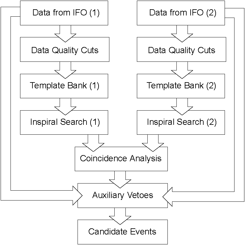
Figure 1: A simple pipeline used to search data from two interferometers for inspiral signals. Raw data from interferometer, labeled $1$ and $2$, is recorded at the observatories. Data quality cuts are then applied to the raw data to discard times when the interferometer was not in a stable operating mode. Power spectra generated from the data are used to generate a template bank for the inspiral population being searched for. The template banks and interferometer data are used to generate inspiral triggers for each interferometer. The triggers for each interferometer are tested for coincidence, as a true inspiral signal should be present in both interferometers at the same time, up to the time it takes a gravitational wave to travel between the observatories. Other coincidence tests, such as waveform parameter consistency, can be applied at this stage. Transient noise sources may be detected in auxiliary interferometer channels, for example seismometers. Such channels may be used to veto triggers that survive the coincidence analysis but are coincident with the signature of noise in the auxiliary channel. Finally we obtain a sample of candidate events for further investigation. Each step of the pipeline has many parameters that can be tuned to minimize the false alarm and false dismissal rates.

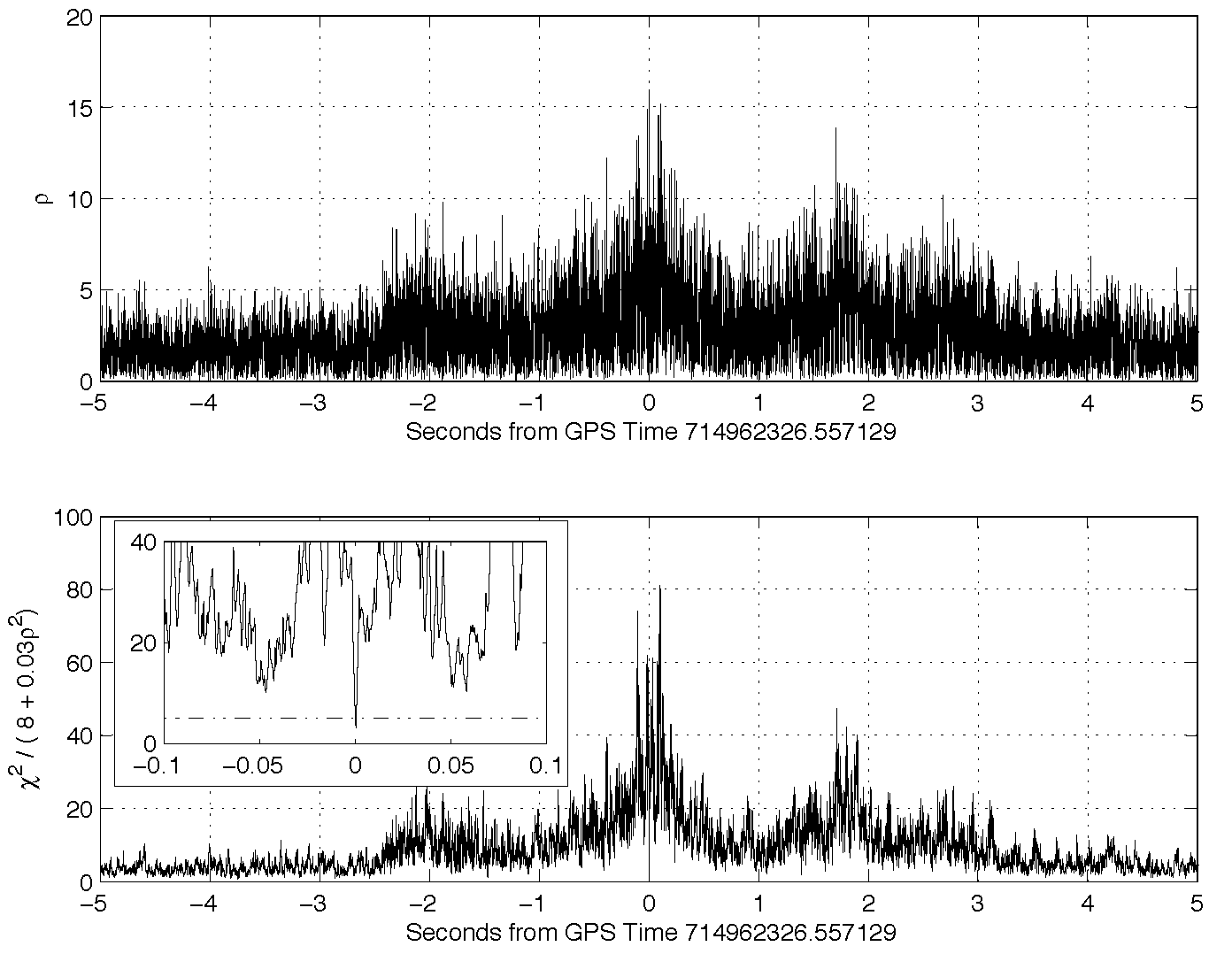
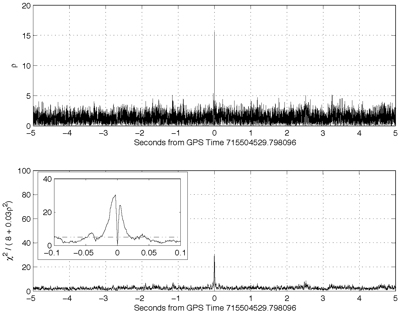
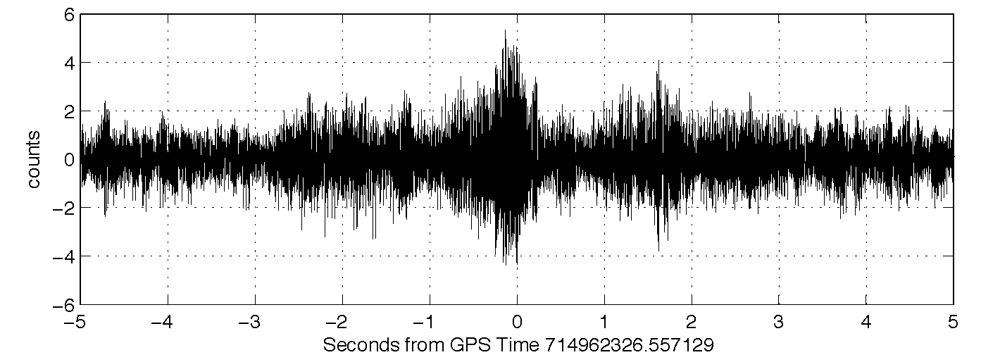
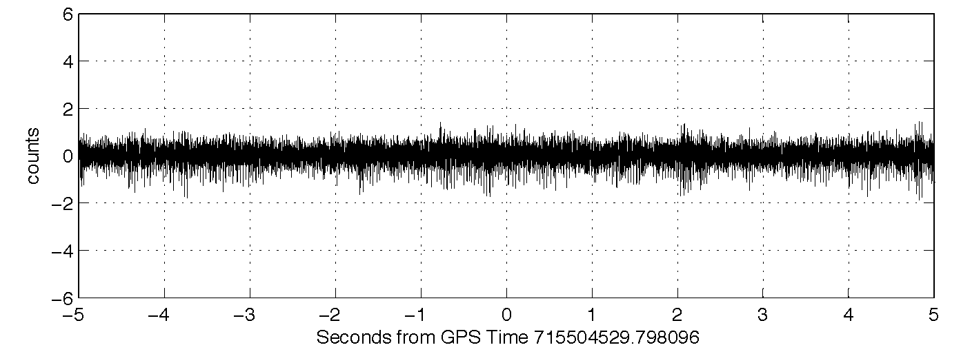
Figure 2: Left Panels: The largest signal-to-noise ratio candidate event seen during the search of the LIGO S1 data. The top panel shows the signal-to-noise time series, $\rho(t)$. Notice that $\rho(t)$ is greater than the S1 threshold of $6.5$ many times in a $\sim 5$ second interval around the candidate event. The center panel shows $\chi^{2}/(p+\delta^{2}\rho^{2})$ as a function of time for the values of $\delta^{2}=0.03$ and $p=8$ used in S1. Notice $\chi^{2}/(p+0.03\rho^{2})$ is greater than the threshold of $5$ for $\sim 5$ seconds around the candidate event, but drops below this threshold right at the time of maximum $\rho$. The inset shows this more clearly for $\pm 0.1$ second around the event where the threshold is indicated by a dot-dashed horizontal line. The bottom panel shows the time series for this candidate event after applying a high-pass filter with a knee frequency of 200 Hz. Notice the bursting behavior which does not look like an inspiral chirp signal. Right Panels: A simulated injection into the L1 data. This example was chosen for comparison with the largest signal-to-noise ratio event shown in the left panels since it similar in mass parameters, detected signal to noise and $\chi^{2}$. The instrument was behaving well at the time around the simulated injection. The top panel shows that $\rho(t)<6.5$ except in close proximity to the signal detection time. The center panel shows $\chi^{2}/(p+0.03\rho^{2})$ as a function of time. Notice that it is much closer to threshold at all times around the simulated injection; this contrasts dramatically with the case of the candidate event shown in the left panels. The inset shows this more clearly for $\pm 0.1$ seconds around the injection. The bottom panel shows the time series for this simulated injection after applying a high-pass filter with a knee frequency of 200 Hz. The inspiral chirp signal is not visible in the noisy detector output.

Mandatory Data Quality Cut	Description
OUTSIDE_S2	Data is outside of official S2 time interval
MISSING_RAW	Raw data is missing
DAQ_DROPOUT	Dropout in data acquisition system
MISSING_RDS	Data is unavailable for analysis
INVALID_TIMING	Timing believed to be unreliable
CALIB_LINE_NO_RDS_V03	Problem with accessing data for calibration
DAQ_REBOOT	One or more data acquisition system rebooted
INVALID_CALIB_LINE	Problem with calibration line strength
NO_CALIB	Calibration line turned off
LOW_CALIB	Calibration line strength too low
Discretionary Data Quality Cut	Description
MICH_FILT	One or more Michelson control loop
	filters was not in its nominal state
AS_PD_SATURATION	Antisymmetric port photodiode saturated
ASQ_LARGEP2P	Large peak-to-peak range seen in AS_Q
	at end of lock
NONSTAND_CTRLS	Non-standard controls affecting calibration
	and couplings
ASQ_OUTLIER_CLUSTER	Cluster of large AS_Q outliers
	in short time interval
ASQ_OUTLIER_CORRELATED	Large ASQ outliers correlated with
	outliers in auxiliary IFO channel
ASQ_LOWBAND_OUTLIER	High noise below 100 Hz in AS_Q
ASQ_UPPERBAND_OUTLIER	High noise in 100-7000 Hz in AS_Q

Table 1: Data quality cuts available during the S2 science run and their meanings. Some data quality flags monitor human error in the operation of the instrument that make the data unsuitable for analysis, such as NO_CALIB and NONSTAND_CTRLS. Others cuts identify hardware or software failures in the operation of the instrument, for example MISSING_RAW and DAQ_REBOOT. Additional cuts like AS_PD_SATURATION and ASQ_UPPERBAND_OUTLIER monitor the gravitational wave channel, AS_Q, for unusable data.

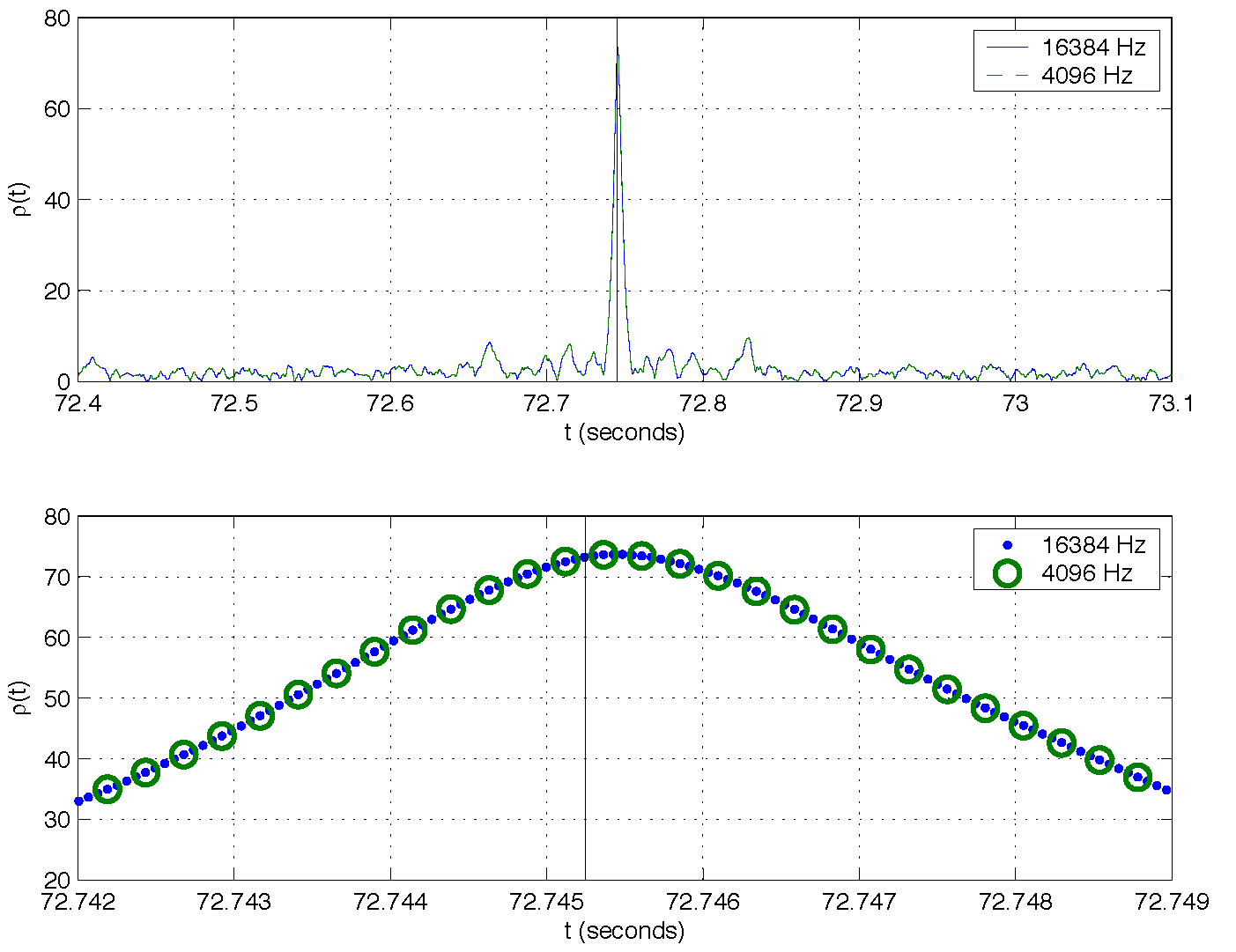
Figure 3: The loss in signal-to-noise ratio for a $0.2,0.2\,M_{\odot}$ black hole MACHO binary due to resampling. The inspiral waveform is generated at $16\,384$ Hz and injected into data with a typical S2 noise curve. The end time of the waveform is at $72.74525$ seconds, shown by the vertical line in both plots. The top panned shows the signal-to-noise ratio for the data segment when using data at the full bandwidth and data resampled to $4096$ Hz. The bottom panel shows the same data close to the end time of the injection. The loss in signal-to-noise ratio for the inspiral trigger generated at $4096$ Hz is $0.1\%$.

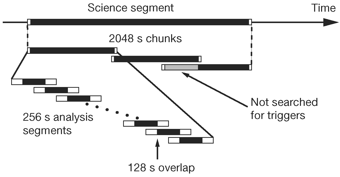
Figure 4: The algorithm used to divide science segments into data analysis segments. Science segments are divided into $2048$ s chunks overlapped by $128$ s. (Science segments shorter than $2048$ s are ignored.) An additional chunk with a larger overlap is added to cover any remaining data at the end of a science segment. Each chunk is divided into $15$ analysis segments of length $256$ s for filtering. The first and last $64$ s of each analysis segment is ignored, so the segments overlap by $128$ s. Areas shaded black are filtered for triggers by the search pipeline. The gray area in the last chunk of the science segment is not searched for triggers as this time is covered by the preceding chunk, however this data is used in the PSD estimate for the final chunk.

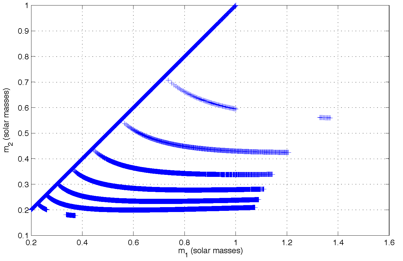
Figure 5: The template bank required to cover the binary black hole MACHO parameter space from $0.2$ to $1$ $M_{\odot}$ at a minimal match of $95\%$. The template bank is generated from the average power spectral density of a typical S2 analysis chunk (starting at GPS time 734256712.) The large number of templates in the BBHMACHO bank is due to the lager number of cycles of the MACHO templates in the sensitive band of the interferometer. The placement of templates outside the mass parameter space is required to ensure that any signal that lies in the space has a minimal match $>0.95$.

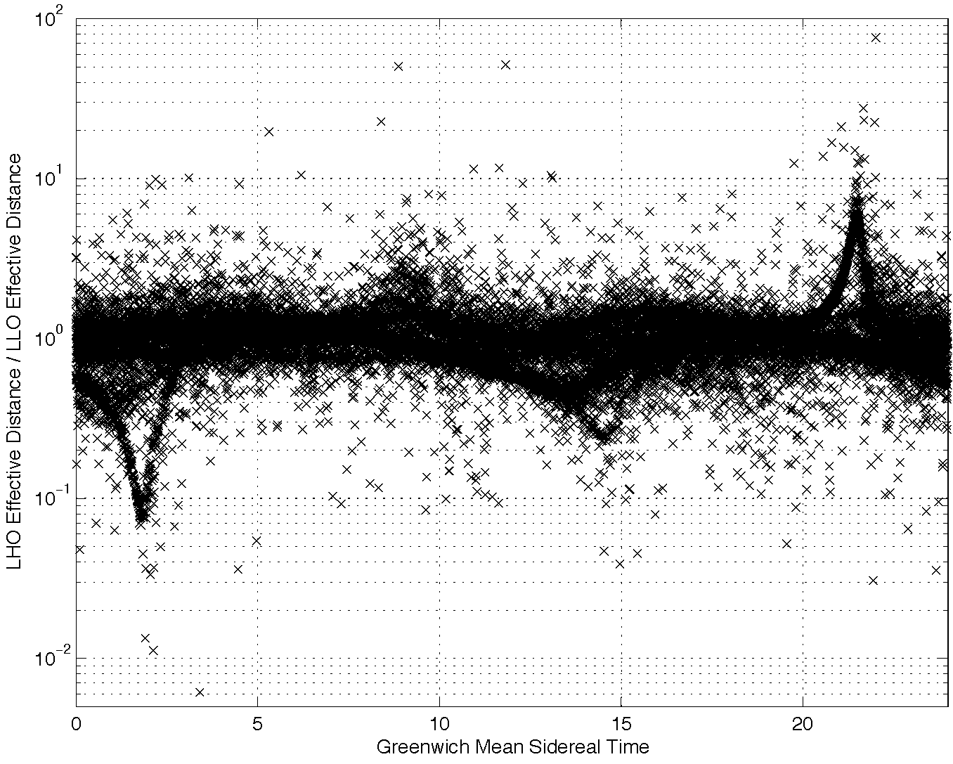
Figure 6: The ratio of the known effective distance of an injected signal in the Hanford Observatory (LHO) to the known effective distance of an injected signal in the Livingston Observatory (LLO) as a function of Greenwich Mean Sidereal Time. The slight misalignment of the interferometers at the two different observatories due to the curvature of the earth causes the antenna pattern of the detectors to differ. As a result the distance at which a binary system appears is different in each detector, even in the absence of noise. The ratio of effective distances can be significant, so this precludes the use of an amplitude cut when testing for inspiral trigger coincidence between different observatories.

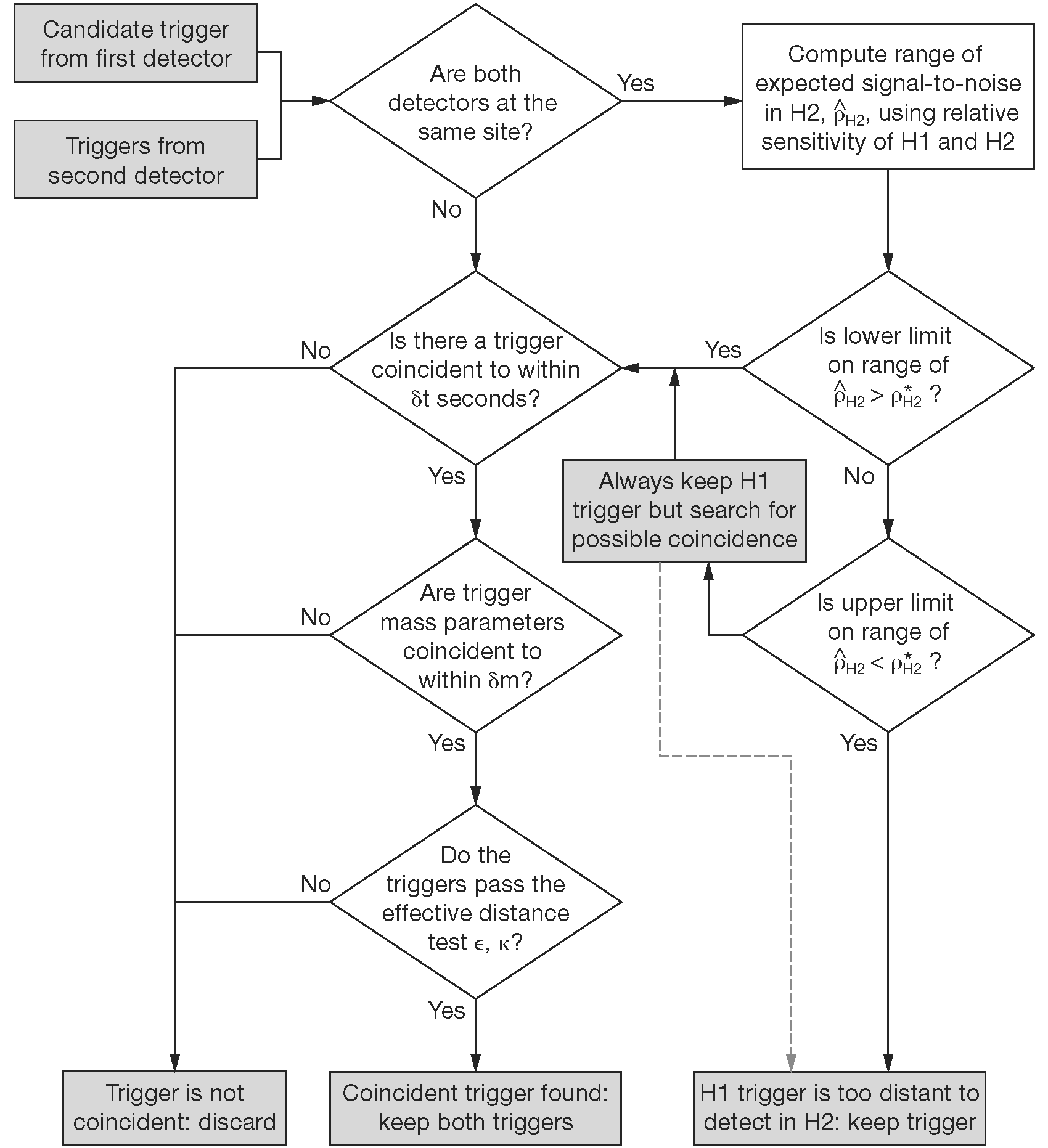
Figure 7: The test to decide if a trigger in the first detector has a coincident trigger in the second detector. If detectors are at different sites, time and mass coincidence are demanded. The effective distance cut is disabled by setting $\kappa=1000$. If the detectors are at the same site, we ask if the maximum distance to which H2 can see at the signal-to-noise threshold $\rho_{\mathrm{H2}}^{\ast}$ is greater than the distance of the H1 trigger, allowing for errors in the measurement of the trigger distance. If this is the case, we demand time, mass and effective distance coincidence. If distance to which H2 can see overlaps the error in measured distance of the H1 trigger, we search for a trigger in H2, but always keep the H1 trigger even if no coincident trigger is found. If the minimum of the error in measured distance of the H1 trigger is greater than the maximum distance to which H2 can detect a trigger we keep the H1 trigger without searching for coincidence.

(i)	(ii)
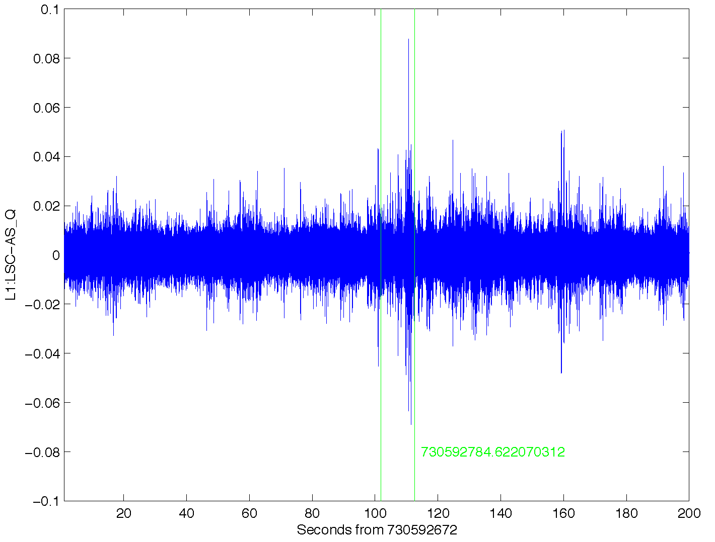
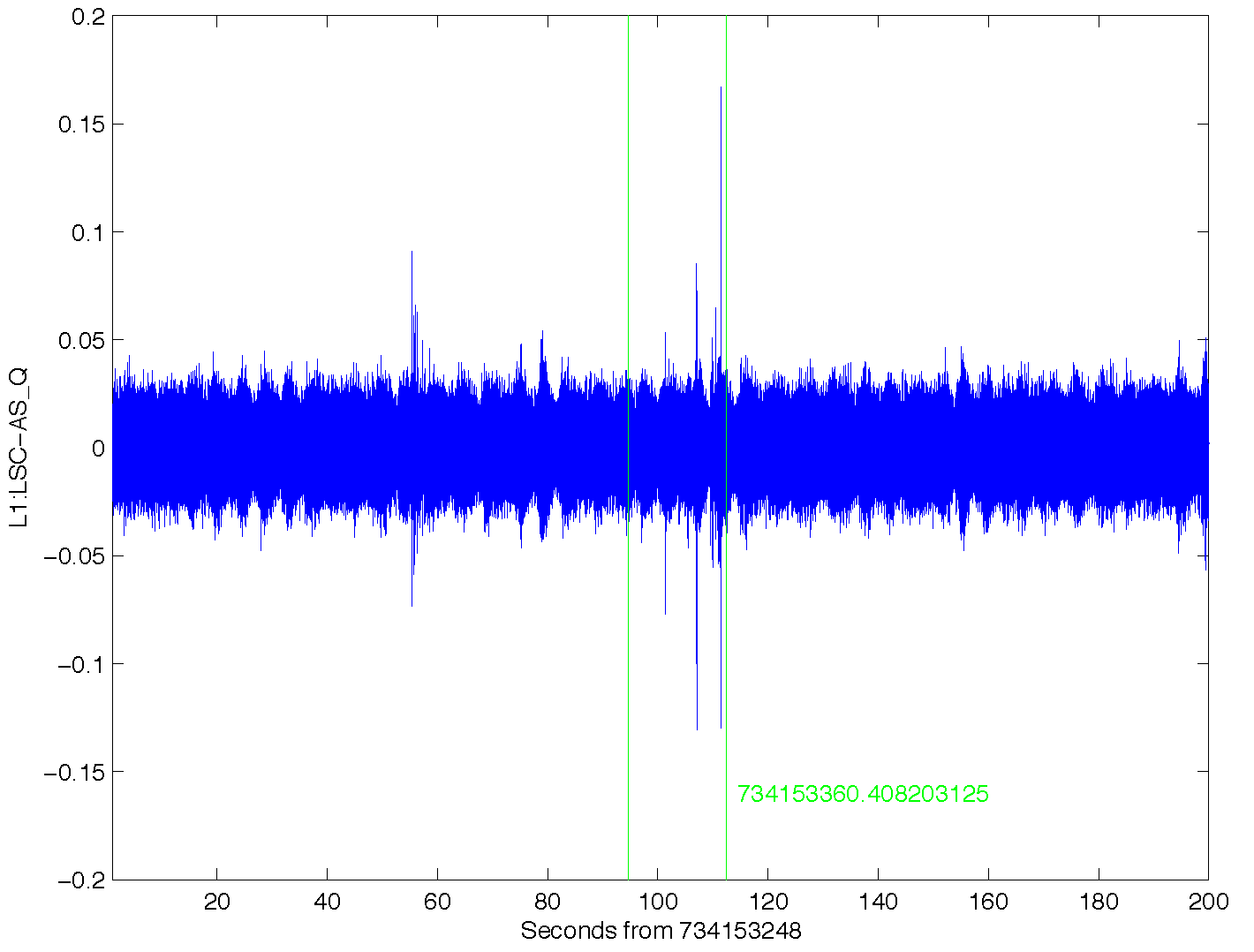
(iii)	(iv)

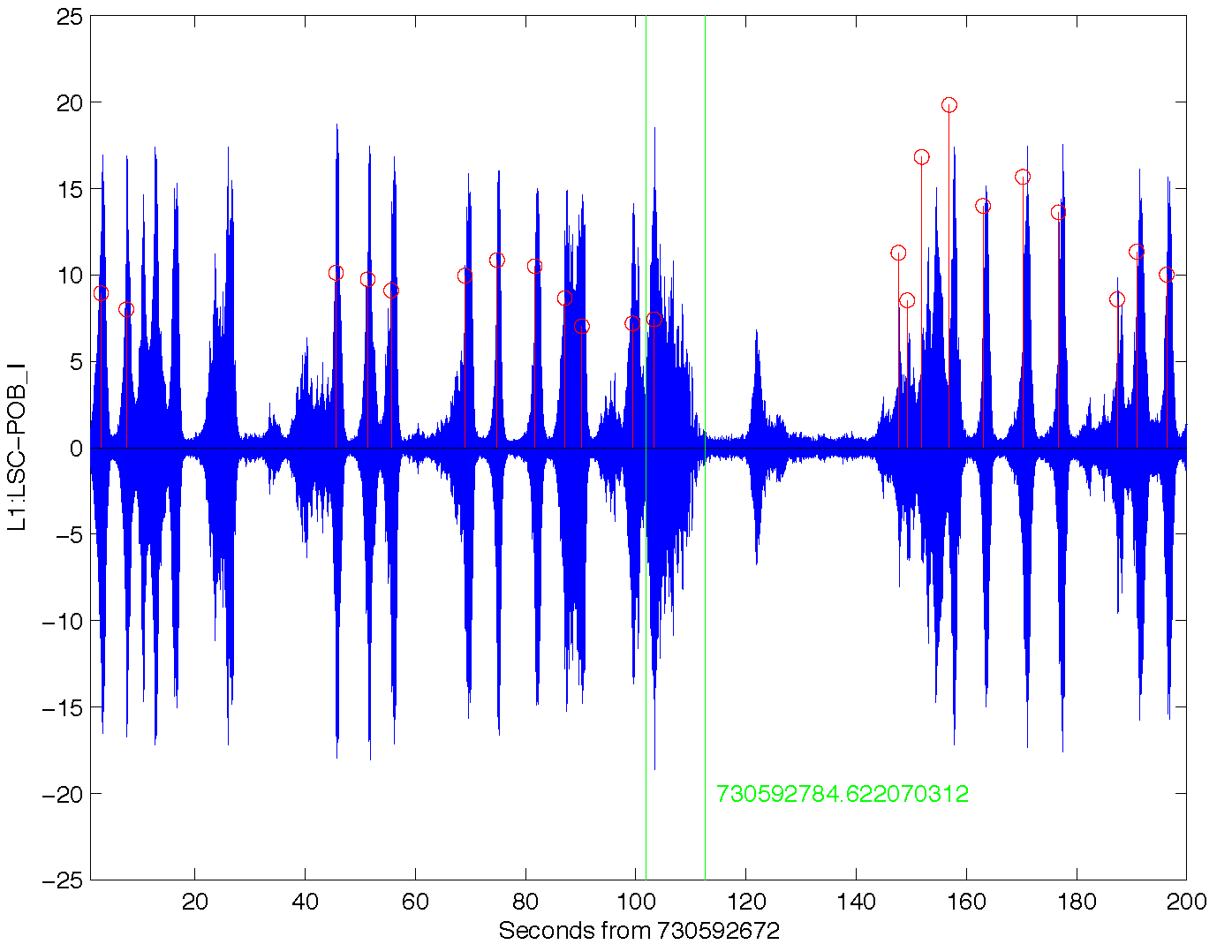
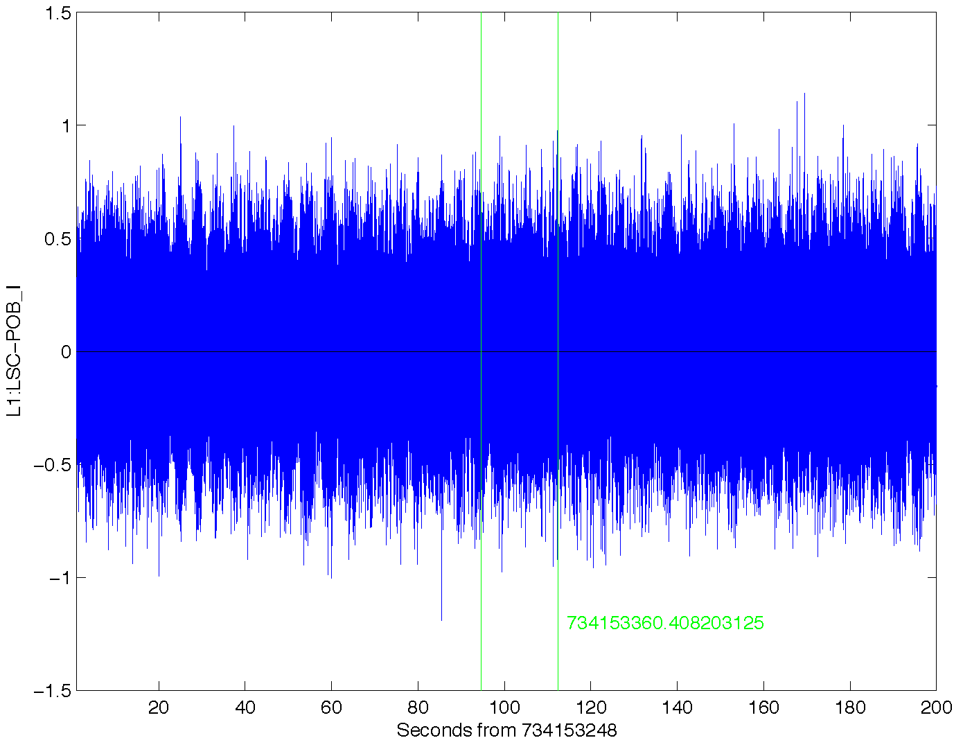
Figure 8: An auxiliary channel veto investigation of two candidate triggers. Panel (i) shows the gravitational wave channel, L1:LSC-AS_Q, high passes above 100 Hz for a an inspiral trigger at GPS time 730592784 with a signal-to-noise ratio $\rho=10.6$. The vertical line shows the time of the inspiral trigger. Panels (iii) shows the auxiliary interferometer channel L1:LSC-POB_I high passed above 70 Hz. The vertical lines with circles show the location of glitchMon triggers produced by the noise in L1:LSC-POB_I. By excluding inspiral triggers within a time window of these glitchMon triggers, we can reduce the number of false event candidates in the pipeline. For contrast, panel (ii) shows an gravitational wave channel high passed above 100 Hz for an inspiral trigger at GPS time 734153360. This trigger has a similar signal-to-noise ratio, $\rho=10.9$, as the trigger in panel (i). For this trigger there does not seem to be a correlated noise source in the auxiliary channel L1:LSC-POB_I shown high passed above 70 Hz in panel (iv).

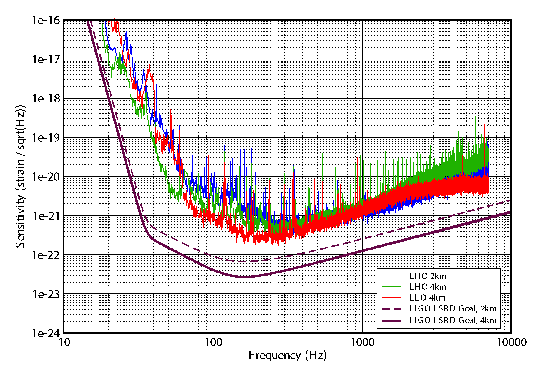
Figure 9: Typical sensitivities of the three LIGO interferometers during the second LIGO science run shown as strain amplitude spectral density, $\tilde{h}/\sqrt{\mathrm{Hz}}$. The smooth solid curve shows the design sensitivity (SRD Goal) of the $4$ km interferometers and the smooth dashed curve shows the design sensitivity of the $2$ km interferometer.

H1 Data Quality Cut	$T_{\mathrm{total}}$	$T_{\mathrm{play}}$	$T_{\mathrm{done}}$	$\rho>8$	$\rho>10$	$\rho>12$
(1)	(2)	(3)	(4)	(5)	(6)	(7)
ASQ_LOWBAND_OUTLIER	14741	1990	1536	625	178	2
ASQ_OUTLIER_CLUSTER	20407	1800	1800	0	0	0
ASQ_OUTLIER_CORRELATED	3126	558	456	390	167	2
ASQ_UPPERBAND_OUTLIER	22817	1876	1876	15435	10159	7574
AS_PD_SATURATION	72	5	0	0	0	0
MICH_FILT	118807	11400	11400	4443	3922	3185
H2 Data Quality Cut	$T\mathrm{total}$	$T_{\mathrm{play}}$	$T_{\mathrm{done}}$	$\rho>8$	$\rho>10$	$\rho>12$
(1)	(2)	(3)	(4)	(5)	(6)	(7)
AS_PD_SATURATION	4	0	0	0	0	0
MICH_FILT	64368	6570	5648	1294	164	7
L1 Data Quality Cut	$T\mathrm{total}$	$T_{\mathrm{play}}$	$T_{\mathrm{done}}$	$\rho>8$	$\rho>10$	$\rho>12$
(1)	(2)	(3)	(4)	(5)	(6)	(7)
ASQ_LARGEP2P	2699	380	0	0	0	0
ASQ_OUTLIER_CORRELATED	840	60	60	0	0	0
AS_PD_SATURATION	646	61	10	813	119	6
MICH_FILT	203539	21696	17794	6393	497	32
NONSTAND_CTRLS	4020	843	18	0	0	0

Table 2: The table shows the inspiral triggers generate from science mode data with the mandatory data quality cuts applied. For each discretionary data quality cut applied a given interferometer (1), the amount of time that would be excluded from the total science mode data by the cut is given (2). Since we tune data quality cuts on playground data, the amount of playground time excluded is also shown (3) and the amount of playground data analyzed for triggers (4). These may differ for reasons explained in section 5.3.2. The number inspiral triggers generated when a particular data quality cut is active is shown for different signal-to-noise thresholds (5–7). To generate the triggers, interferometer data was high passed above $50$ Hz in the time domain and a low frequency cutoff of $70$ Hz was applied to frequency domain. Template banks were generated with a minimal match of $0.97$ and the signal-to-noise threshold for the matched filter was set to $\rho_{\ast}=8$. A $\chi^{2}$ veto with $8$ bins applied with a threshold of $\chi^{2}<20(8+0.03^{2}\rho^{2})$.

Discretionary Data Quality Cut	Applied
MICH_FILT	No
The cut would exclude a large number of triggers, but would reduce the amount of data in the search significantly. It was decided not to apply this cut and to try and exclude false triggers from these times by a combination of coincidence, vetoes and reducing the $\chi^{2}$ threshold.
AS_PD_SATURATION	Yes
Clear correlation with inspiral triggers with large signal-to-noise ratios in L1 and the study described in section 5.2.1 suggest that this should be used. The lack of correlated trigger in H1 was due to the fact that the playground did not sample any times with photodiode situations.
ASQ_LARGEP2P	No
A loud inspiral signal could trigger this cut, so it is unsafe for use.
NONSTAND_CTRLS	Yes
Advice from experimental team advised that detections made during this time could not be trusted.
ASQ_OUTLIER_CLUSTER	No
Not well correlated with inspiral triggers.
ASQ_OUTLIER_CORRELATED	No
Not well correlated with inspiral triggers.
ASQ_LOWBAND_OUTLIER	No
Not well correlated with inspiral triggers.
ASQ_UPPERBAND_OUTLIER	Yes
Times with high upper band noise in H1 are clearly correlated with high signal-to-noise ratio triggers. In order to prevent the cut from begin triggered by real signals we also require that the cut is on for more that $180$ seconds. The longest inspiral signal in the S2 analysis is $52$ seconds.

Table 3: The final selection and justification of discretionary data quality cuts for the S2 binary neutron star and binary black hole MACHO searches.

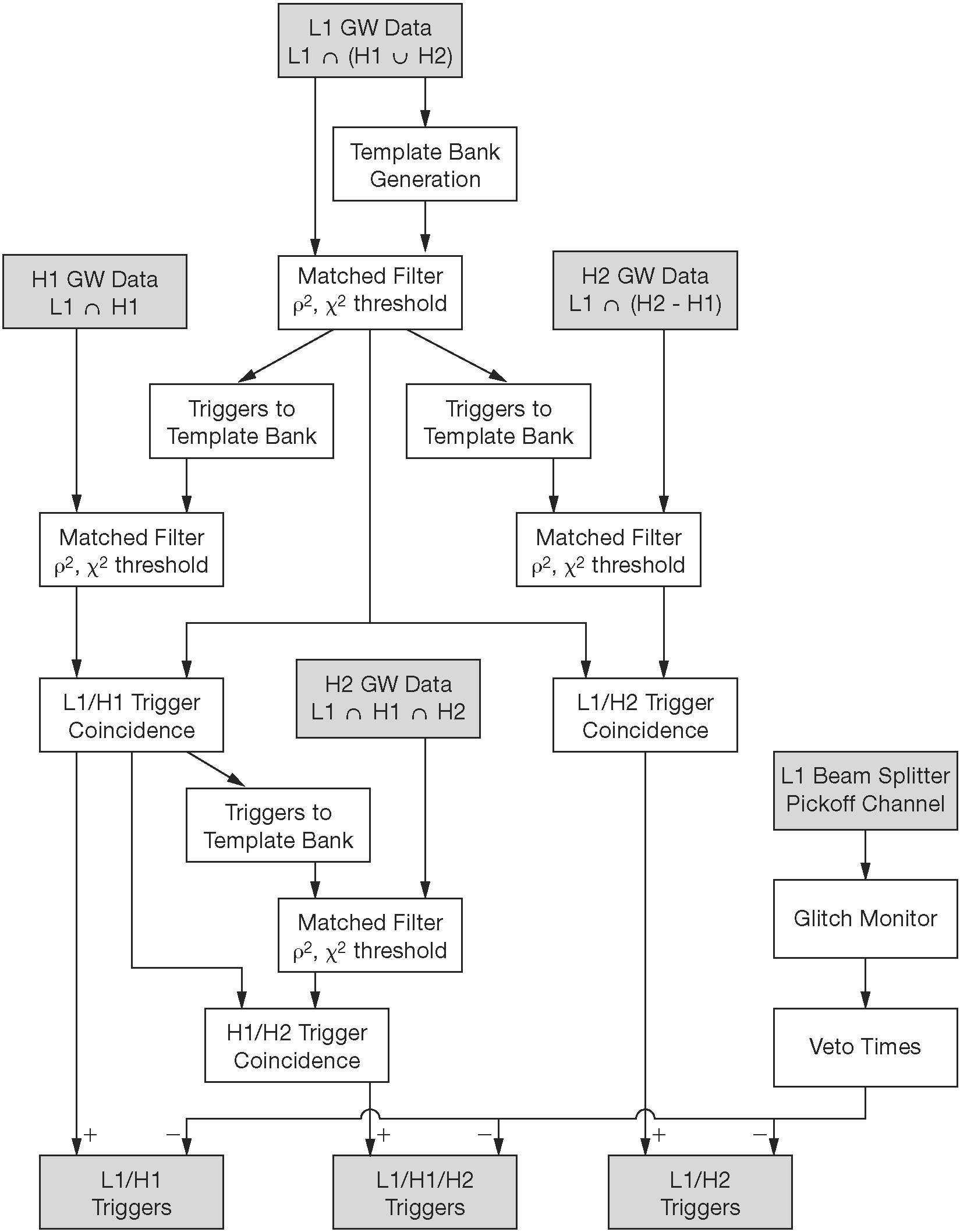
Figure 10: The inspiral analysis pipeline used to determine the reported upper limit. $\mathrm{L1}\cap(\mathrm{H1}\cup\mathrm{H2})$ indicates times when the L1 interferometer was operating in coincidence with one or both of the Hanford interferometers. $\mathrm{L1}\cap\mathrm{H1}$ indicates times when the L1 interferometer was operating in coincidence with the H1 interferometer. $\mathrm{L1}\cap(\mathrm{H2}-\mathrm{H1})$ indicates times when the L1 interferometer was operating in coincidence with only the H2 interferometer. The outputs of the search pipeline are triggers that belong to one of the two double coincident data sets or to the triple coincident data set.

Interferometer	Start	End	Duration
L1	730000000	730010000	10000
L1	731001000	731006000	5000
L1	732000000	732003000	3000
H1	730004000	730013000	8000
H1	731000000	731002500	2500
H1	732000000	732003000	3000
H2	730002500	730008000	5500
H2	731004500	731007500	2500
H2	732000000	732003000	3000

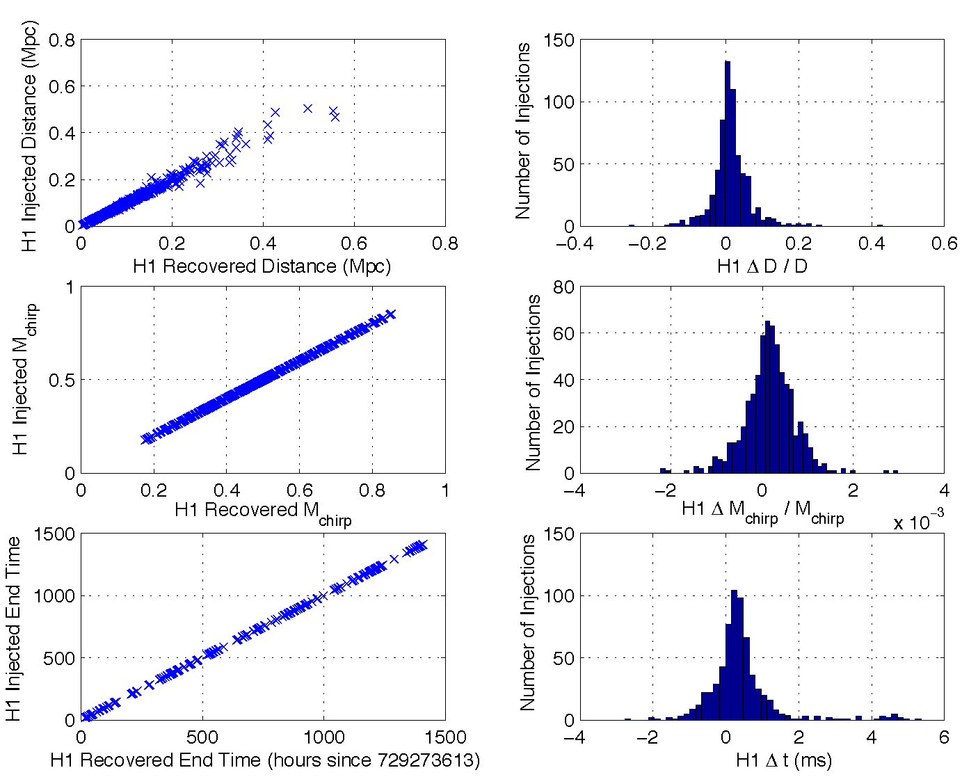
Figure 11: The panels in this figure compare the measured values of effective distance, chirp mass and end time with the known values for the injected waveforms in the Monte Carlo simulation in the H1 detector.

Table 4: The fake science segments used to construct the DAG shown in figure 11.

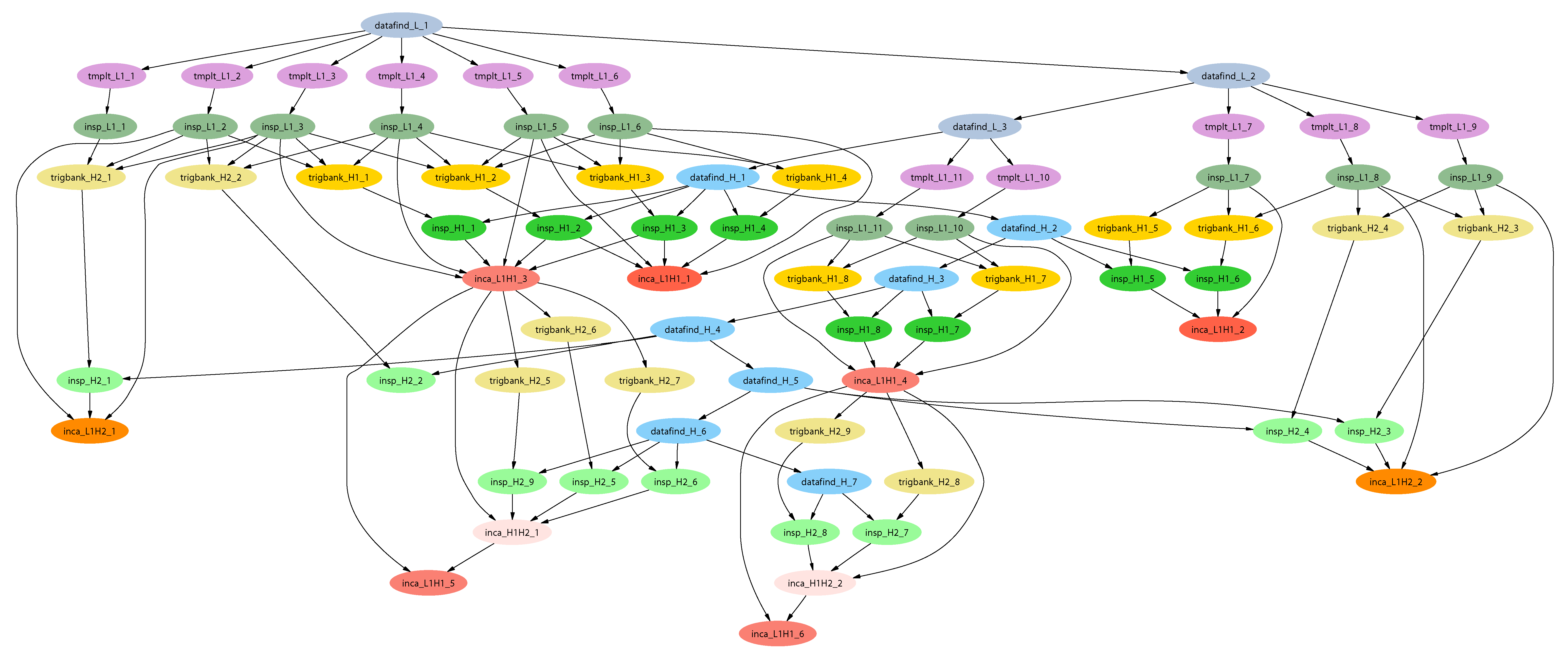
Figure 11: The DAG generated from the pipeline shown in figure 10 and the fake science segment list described in section 5.8.3. The figure shows the structure of the DAG with all job dependencies needed to execute the S2 pipeline. Note that it appears that there are several LHO master chunks analyzed that do not need to be filtered for a zero time lag. These are added to the DAG to ensure that all the data necessary for a background estimation with a maximum time side of 500 seconds is analyzed.

Chapter 6 Hardware Signal Injections

Gravitational radiation incident on the LIGO interferometers from an inspiralling binary will cause the test masses to move relative to each other. This produces a differential change in length of the arms as described in section 2.1. Injection is the process of adding a waveform to interferometer data to simulate the presence of a signal in the noise. We use injections to measure the performance of the binary inspiral analysis pipeline as described in section 5.7. Software injections, which add a simulated signal to the data after it has been recorded, are used for efficiency measurements. Since they performed a posteriori the interferometer is not affected while it is recording data. Alternatively, a simulated signal can be added to the interferometer control system to make the instrument behave as if an inspiral signal is present. The interferometer Length Sensing and Control system has excitation points which allow arbitrary signals to be added into the servo control loops or to the drives that control the motion of the mirrors[LIGOS1instpaper]. We call this hardware injection; the data recorded from the instrument contains the simulated signal. Figure 1 shows the hardware injection points on a schematic diagram of the interferometer and length sensing and control loop.

Analysis of hardware injections allows us to ensure that the analysis pipeline is sensitive to real inspiral signals and validates the software injections used to test the pipeline efficiency. In order to perform an accurate upper limit analysis for binary inspirals, we must measure the efficiency of our pipeline. That is, we inject a known number of signals into the pipeline and determine the fraction of these detected. Injecting signals into the interferometer for the duration of a run is not practical and would contaminate the data, so we use the analysis software to inject inspiral signals into the data. By comparing software and hardware injections we confirm that software injections are adequate to measure the efficiency of the upper limit pipeline.

Hardware injections provide a very complete method of testing the inspiral detection pipeline. By recovering the physical parameters of an injected signal, we test our understanding of all aspects of the pipeline, including the instrumental calibration, the filtering algorithm and veto safety. We injected inspiral signals immediately after the first LIGO science run (S1) in September 2002. The resulting data was analyzed using the software tools used to search for real signals. In this chapter, we describe the results of analysis of the S1 hardware injections. The analysis pipeline used in S1 differs from that used in S2[LIGOS1iul]. Here we are examining the response of the filtering code to the hardware injections, however, and so the differences between the S1 and S2 pipelines are unimportant.

6.1 Injection of the Inspiral Signals

To inject the signals, we generate the interferometer strain $h(t)$ produced by an inspiralling binary using the restricted second order post-Newtonian approximation in the time domain[Blanchet:1996pi]. The LSC calibration group supplies a transfer function $T(f)$ which allows us to construct a signal $g(t)$ that produces the desired strain when it is injected into the interferometer. The transfer function $T(f)$ should be identical to the actuation function $A(f)$ described in section 2.2.3, however in S1 this was simplified to contain only the pendulum response of the mirrors, given by

$$T(f)=\frac{L}{C}\frac{f^{2}}{f_{0}^{2}}$$ (6.1)

where $L$ is the length of the interferometer, $C$ is the calibration of the excitation point in nm/count and $f_{0}$ is the pendulum frequency of the test mass. Damping is neglected as it is unimportant in the LIGO frequency band. The code used to generate the hardware injections is the same as that used for software injections; only the transfer function used to generate the injected signal differs since we are injecting into the control signal $g$ rather than the error signal $v$.

During S1, we injected signals corresponding to an optimally oriented binary. Injections of a $1.4\,M_{\odot}$ inspiralling binary at distances from $10$ kpc to $80$ kpc were used to test the neutron star analysis. We also injected signals from a $1.4,\,4.0\,M_{\odot}$ binary and several $1.4,1.4\,M_{\odot}$ binaries at closer distances. These signals were injected into the differential mode servo and directly into an end test mass drive.

6.2 Detection of the Injected Signals

Figure 2 shows the events generated by processing 4000 seconds of data from the Livingston 4 km interferometer (L1) on 10 September 2002 during the post-run hardware injections.

The first set of injections were large amplitude signals used to verify the inspirals were being correctly injected. We ignore these and concentrate on the second set, which were at more appropriate distances. We only consider the 1.4 solar mass inspiral injections, as the 1.4,4.0 injection lies outside the template bank space used in the S1 binary neutron star analysis.

It can be seen that all of the hardware injections are identified as candidate events since they have high signal-to-noise ratios and values of the $\chi^{2}$ test lower than $5$, which was the threshold used in the S1 analysis pipeline[LIGOS1iul]. Some of the 1.4,4.0 injections are also flagged for further investigation as they cause templates inside the bank to ring, but have high $\chi^{2}$ values as they are not exactly matched.

Since we know the exact coalescence time of the injected waveform, we can compare this with the value reported by the search code and ensure that the search code is reporting the correct time. The known and measured parameters for the second set of $1.4,1.4\ M_{\odot}$ injections are shown in table 1. The raw data is resampled to $4096$ Hz before being filtered. For each of the signals injected, we were able to detect the coalescence time of the injection to within one sample point of the correct value at $4096$ Hz, which is consistent with the expected statistical error and confirms that the pipeline has not introduced any distortion of the signals.

6.3 Checking the Instrumental Calibration

Calibration measurements of the interferometers were performed before and after the run; these are the reference calibrations. In general, the calibration changes due to changes in the alignment on time scales of minutes. This variation is encoded in the parameter $\alpha$ which is monitored using a sinusoidal signal injected into the detector (see section 2.2.3). $\alpha$ is used as input to the data analysis pipeline and varied between $0.4$ and $1.4$ during S1. Data in S1 was analyzed in 256 second segments. For each 256 seconds of data starting at time $t_{0}$, we construct the calibration, $R(f;t_{0})$ by using $\alpha(t_{0})$ and a reference calibration. $R(f;t_{0})$ is then used to calibrate the 256 seconds of data.

Figure 3 shows a set of injections into the Livingston interferometer analyzed with different calibrations generated by varying the value of $\alpha$. We expect that the signal-to-noise varies quadratically and the effective distance varies linearly with changes in $\alpha$[Allen:1996]. This is confirmed by the injections. There is no single value of $\alpha$ that gives the correct effective distance for all the injections; this is consistent with the estimated systematic errors in the calibration. Unfortunately the calibration line was not present during the time the hardware injections were performed, so we cannot directly compare a measured calibration with the result of the injections.

6.4 Safety of Vetoes

During construction of the the inspiral pipeline we considered using inspiral triggers found in auxiliary interferometer channels as vetoes on triggers in the gravitational wave channel. Concern was raised that a real inspiral signal may couple between these channels and a real signal may be inadvertently vetoed. To check this, we examined coupling between the channels at the time of an injection. Figure 4 shows the power spectra of the gravitational wave channel, LSC-AS_Q, and the auxiliary channels that we considered using as vetoes during S1: LSC-AS_I, LSC-REFL_I and LSC-REFL_Q. The injected inspiral signal can clearly be seen coupling to the auxiliary channel LSC-AS_I, but there is no obvious coupling between the injected signal and LSC-REFL_I or LSC-REFL_Q. This led us to discard LSC-AS_I as a possible veto channel in the S1 analysis. Similar studies have been performed for the S2 data when auxiliary channels are proposed as veto channels.

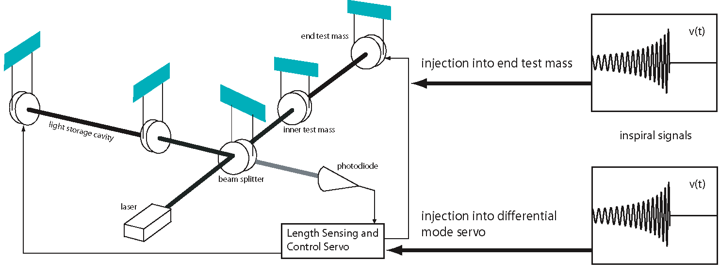
Figure 1: A schematic diagram of the LIGO interferometer showing the injection points used in S1 hardware injections. Inspiral signals were injected either directly into the end test mass drive of one arm or into the differential mode servo, and this into both arms. Care was taken to ensure that the correct transfer function, $T(f)$, was used in each case.

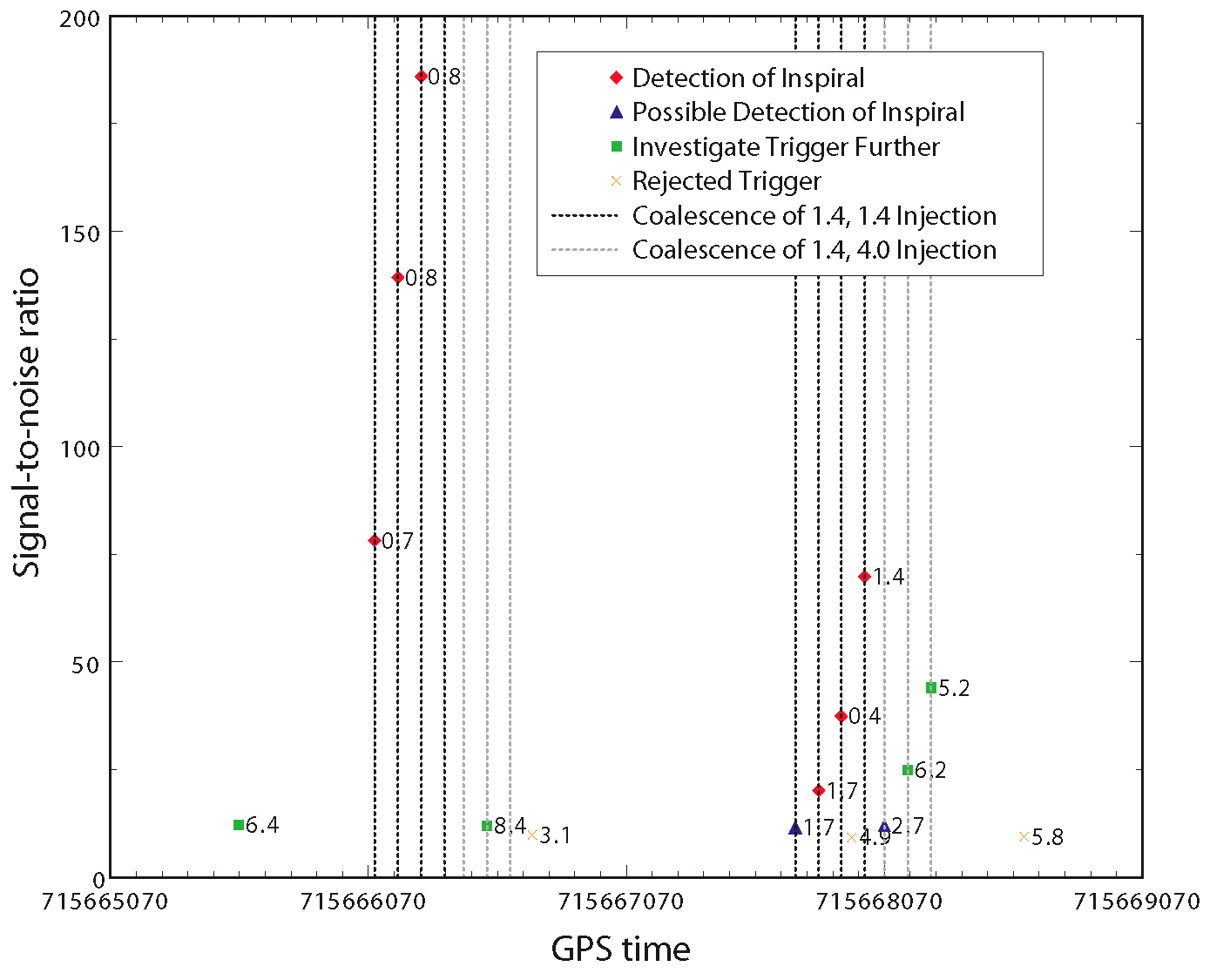
Figure 2: The candidate events generated by processing 4000 seconds of data from the Livingston 4 km interferometer through the S1 analysis pipeline. This data included two sets of injections; the known coalescence times are indicated by the dashed vertical lines. The signal-to-noise ratio is plotted and the value of the $\chi^{2}$ veto is shown next to the candidate event.

End time of Injection	End Time of Detection	$\rho$	$\chi^{2}$
$04:35:12.424928$	$04:35:12.424927$	$11.623546$	$1.653222$
$04:36:42.424928$	$04:36:42.425171$	$20.230101$	$1.671016$
$04:38:12.424928$	$04:38:12.424927$	$37.488770$	$0.443966$
$04:39:42.424928$	$04:39:42.424927$	$69.815262$	$1.375486$

Table 1: Hardware injection events found by the inspiral analysis pipeline. End time of injection is the known end time of the injected signal and end time of detection is the end time of the signal as reported by the analysis pipeline. Times are Universal Time (UTC) on 10 September 2002. The values of signal-to-noise ratio $\rho$ and $\chi^{2}$ veto are given for each event.

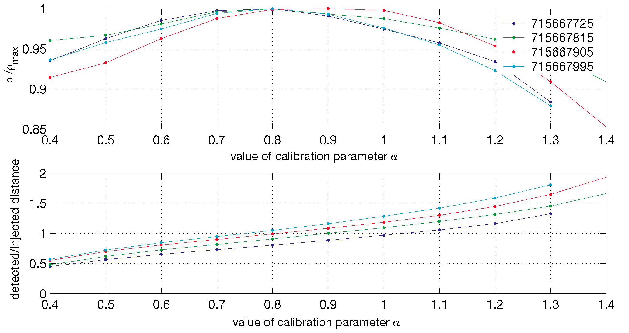
Figure 3: Each curve corresponds to a hardware injection at the given GPS time. We re-analyze each injection with different calibrations to show how the detected quantities vary with $\alpha$. The upper plot shows the ratio of signal-to-noise ratio, $\rho$, to its maximum value, $\rho_{\mathrm{max}}$. The lower plot shows the ratio of the detected distance to the known distance of the hardware injection.

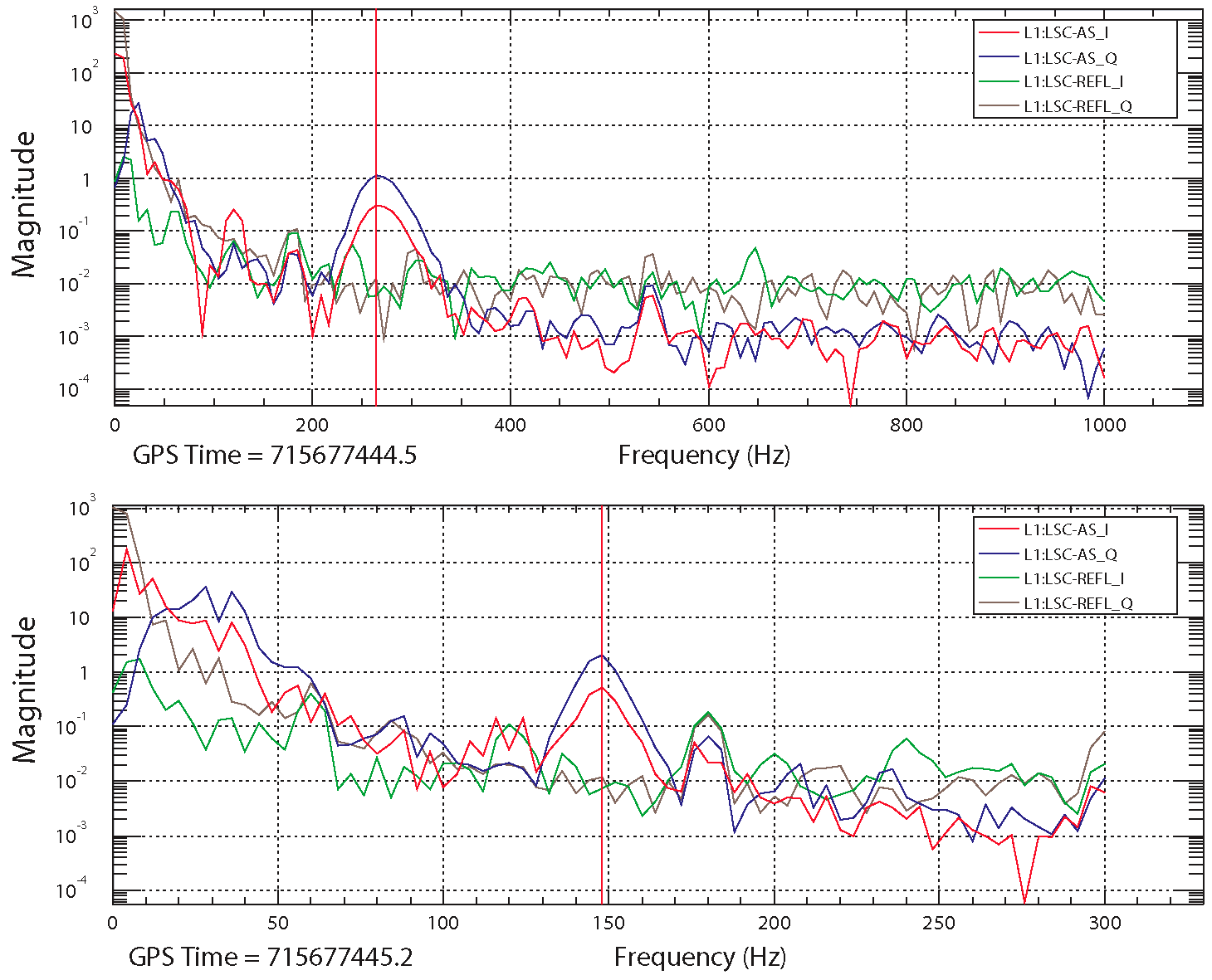
Figure 4: Power spectra of the gravitational wave channel LSC-AS_Q and the auxiliary channels LSC-AS_I, LSC-REFL_I and LSC-REFL_Q during a hardware injection. The broad peak in the spectrum is the inspiral signal and the two power spectra taken at subsequent times show it sweeping across the band as the frequency of the inspiral signal increases with time.

Chapter 7 The Rate of Binary Black Hole MACHO Inspirals in the Halo

In this chapter, we present the results of a search for gravitational waves from the inspiral of binary black hole MACHOs in data from the second LIGO science run (called S2). The goal of the search is the detection of the gravitational waves. In the absence of a detection, however, we place an upper limit on the rate of inspiralling BBHMACHOs. This limit may be compared to the predicted rate of $5\times 10^{-2}\times 2^{\pm 1}$ discussed in chapter 3.

Analysis of the full S2 data set for gravitational waves from inspiralling binary black hole MACHOs is complete and the result of this search will appear in [S2Macho:2004]. Since this result is currently embargoed pending LIGO Scientific Collaboration internal review, we instead present the result of the search on the playground data. No gravitational waves from BBHMACHO inspirals were found in the playground, so in section 7.5 we compute an upper limit on the rate of binary black hole MACHO inspirals in the playground data. Although this result is statistically biased, as it is computed from data used to tune the pipeline, it allows us to make a reasonable prediction of the upper limit available using the full S2 data and assuming no BBHMACHO signals are detected in the full data set.

In section 7.1 we describe the data sample used in the analysis. Section 7.2 describes how the parameters of the search listed in the previous chapter were tuned on the playground data. Section 7.3 described the Monte Carlo simulations used to measure the efficiency of the pipeline. In section 7.4 we describe the background observed in the S2 data.

7.1 The Second LIGO Science Run

All three LIGO detectors operated during the second science run, referred to as S2, which lasted for 59 days (1415 hours) from February 14 to April 14, 2003. Although the detectors were manned by operators and scientific monitors around the clock, the amount of data flagged for scientific analysis was limited by environmental factors (especially high ground motion at LLO and strong winds at LHO), occasional equipment failures, and periodic special investigations. The total amount of science data obtained was 536 hours for L1, 1044 hours for H1, and 822 hours for H2.

The analysis described in this thesis uses data collected while the LLO detector was operating at the same time as one or both of the LHO detectors in order to make use of the triggered search pipeline. Science mode data during which both H1 and H2 were operating but L1 was not, amounting to 383 hours, was not used in this analysis because of concerns about possible environmentally-induced correlations between the data streams of these two co-located detectors. This data set, as well as data collected while only one of the LIGO detectors was in science mode, will be combined with data from the third LIGO science run in a future analysis. Figure 1 shows a breakdown by interferometer of the data recorded during S2. The data used in this search is indicated by the shaded region.

7.2 Tuning the Analysis Pipeline

The entire analysis pipeline was explored first using the playground data set in order to tune the the various thresholds and other parameters. The goal of tuning the pipeline is to maximize the efficiency of the pipeline to detection of gravitational waves from binary inspirals without producing an excessive rate of spurious candidate events. In the absence of a detection, a pipeline with a high efficiency and low false alarm rate allows us to set the best upper limit. It should be noted, however, that our primary motivation is to enable reliable detection of gravitational waves. The efficiency is measured by Monte Carlo simulations in which signals from the hypothetical population are added to the data and then sought. This approach accounts for any systematic error associated with the methods used in our pipeline. Note that another factor in the tuning of the pipeline are the available computational resources. We would like to be able to complete the search in less time than the length of the data being analyzed, so that real-time searches are possible when the interferometers are taking continuous data. For this reason, certain tuning decisions are based on the computational efficiency of the pipeline; these decisions will be clearly identified below.

Prior to commencing the binary black hole MACHO search, a search for inspiralling binary neutron stars (BNS) was conducted on the S2 data using the pipeline described in chapter 5[LIGOS2iul]. The mechanics of the BNS search are very similar to those described here, except that the template bank covers binaries with $1.0\,M_{\odot}<m_{1},m_{2}<3.0\,M_{\odot}$, where $m_{1}$ and $m_{2}$ are the masses of each object in the binary. Since the BNS and binary black hole MACHO searches are very similar, and share the same playground data, we may use the parameters of the BNS search (which were tuned on the playground data) as a starting point for tuning the binary black hole MACHO search.

There are two sets of parameters that we are able to tune in the pipeline: (i) the single interferometer parameters which are used in the matched filter and $\chi^{2}$ veto to generate inspiral triggers in each interferometer, and (ii) the coincidence parameters used to determine if triggers from two interferometers are coincident. The single interferometer parameters include the signal-to-noise threshold $\rho^{\ast}$, the number of frequency sub-bands in the $\chi^{2}$ statistic $p$, the $\chi^{2}$ cut threshold $\Xi^{\ast}$, and the coefficient on the signal-to-noise dependence of the $\chi^{2}$ cut, i.e. $\delta^{2}$ in equation (4.151). These are tuned on a per-interferometer basis, although some of the values chosen are common to two or even three detectors. The coincidence parameters are the time coincidence window $\delta t$ for triggers, the mass parameter coincidence window $\delta m$ and the effective distance cut parameters $\epsilon$ and $\kappa$ in equation. (5.8). Due to the nature of the triggered search pipeline, parameter tuning was carried out in two stages. We first tuned the single interferometer parameters for the primary detector (L1). We then used the triggered template banks (generated from the L1 triggers) to explore the single interferometer parameters for the less sensitive Hanford detectors. Finally the parameters of the coincidence test were tuned.

7.2.1 Template Bank Generation

Recall that the number of templates needed to cover a given region of parameter space at a specified minimal match fluctuates as the shape of the noise power spectrum changes. The greater the sensitivity at low frequencies, relative to higher frequencies, the larger the template bank (see section 5.3.1). The computational resources available for the MACHO search are limited and the computational cost is proportional number of templates in the bank. We therefore tuned the template bank parameters to allow the search to be completed within the available resources.

Due to the algorithm used to construct the template bank[Owen:1998dk], the smallest mass template in the bank will be the equal mass binary $(m_{\mathrm{min}},m_{\mathrm{min}})$, where $m_{\mathrm{min}}$ is the (user specified) minimum binary component mass. Figure 2 shows the size of the template bank necessary to cover each playground analysis chunk at a minimal match of $0.97\%$ for several values of $m_{\mathrm{min}}$. The maximum binary component mass in each case is $1\,M_{\odot}$, so the largest mass binary in the bank parameter space is $(1,1)\,M_{\odot}$. For fixed $m_{\mathrm{min}}$ the number of templates remains reasonably constant over the course of the S2 run, but there is a large variation in the number of templates required as a function of lower mass. The scaling of template number as a function of lower mass is consistent with that described in [Owen:1998dk].

As described in chapter 3, the MACHO mass range measured by microlensing is $0.15\,M_{\odot}$ to $0.9\,M_{\odot}$ at $95\%$ confidence. It would therefore be desirable for the binary black hole MACHO inspiral search to cover a region of mass parameter space slightly larger than this, say $0.1\,M_{\odot}$ to $1.0\,M_{\odot}$. It can be seen, however, that almost an order of magnitude more templates are needed to decrease the lower boundary of the mass parameter space from $0.2\,M_{\odot}$ to $0.1\,M_{\odot}$. Therefore, given the computational resources available for the BBHMACHO search, the lowest mass template in the bank was set to $0.2\,M_{\odot}$. Note that for the final search, the match of the template bank was also lowered to $0.95\%$ to further decrease the number of templates to an average of $14\,179$ per analysis chunk over the S2 run. The latter choice is be justified by the sensitivity to galactic binary black hole MACHOs in S2, as will be seen below. The size of the inspiral template bank used is shown in figure 3.

7.2.2 Interferometer Sensitivity and Signal-to-noise Thresholds

The noise power spectrum also determines the sensitivity of the interferometer to binary inspirals. We can quantify the sensitivity in terms of the distance to which we can see an optimally oriented binary inspiral at a given signal-to-noise ratio. This is the maximum distance at which the interferometer can detect a binary (at this signal-to-noise ratio), since the gravitational wave strain in the interferometer is a maximum when the binary is optimally oriented. The maximum inspiral ranges for an optimally oriented binary at signal-to-noise ratio $\rho^{\ast}=8$ are shown in figure 3. The distance to which we can detect an optimally oriented binary is also a function of the mass of the binary, scaling as $\mu^{1/2}M^{1/3}$; figure 3 shows the ranges for a $(0.5,0.5)\,M_{\odot}$ and a $(0.1,0.1)\,M_{\odot}$ binary.

Notice that there are no times when either of the LHO interferometers are more sensitive than the LLO interferometer and so demanding triggers are always present in the most sensitive interferometer means that they are required to be found in L1. In fact the LLO interferometer has a significantly larger range than either of the LHO interferometers, at times being sensitive to BBHMACHO inspirals in Andromeda at around $0.7$ Mpc. Since we require coincidence between L1 and one of the LHO interferometers to make a detection, however, we are restricted to a search for BBHMACHOs in the Galactic halo.

Based on the sensitivity plots shown in figure 3, we set the signal-to-noise threshold to $7$ in all three interferometers; we justify this as follows. All three interferometers are sensitive to optimally oriented inspirals with $\rho^{\ast}\geq 8$ at distances greater than the size of the Galactic halo. A binary black hole MACHO in the Galaxy may have an unfavorable orientation, however, causing it to appear at a large effective distance. For this reason, we want to set the signal-to-noise ratio threshold as low as possible without producing an excessive false alarm rate. Lowering the signal-to-noise threshold has a computational impact on our search: when the signal-to-noise ratio for a template crosses threshold, we perform the $\chi^{2}$ veto which requires $p$ additional complex inverse FFTs, where $p$ is the number of frequency bins used in the veto. If we set the signal-to-noise threshold too low, we may exceed the available computational resources due to the extra operations required to perform the $\chi^{2}$ veto. In fact this is what happens with the S2 binary black hole MACHO search since the template banks are so large. Whereas in the S2 BNS search we were able to lower the signal-to-noise threshold to $6$, the BBHMACHO search is limited to a signal-to-noise threshold to $7$.

7.2.3 Tuning the $\chi^{2}$ Veto Parameters

Recall from section 4.8.2 that the $\chi^{2}$ veto thresholds on

$$\chi^{2}<\chi^{2}_{\ast}(p+\rho^{2}\delta^{2}),$$ (7.1)

where $\rho$ is the signal-to-noise ratio of the signal and $\delta^{2}$ is a parameter chosen to be reflect the largest expected mismatch that a true signal will have with the templates in the bank. The initial parameters used for the $\chi^{2}$ veto, based on tuning of the BNS search, were $p=15$ and $\delta^{2}=0.04$ with the threshold set to $\chi^{2}_{\ast}(\mathrm{L1})=5.0$ in the L1 interferometer and $\chi^{2}_{\ast}(\mathrm{H1})=\chi^{2}_{\ast}(\mathrm{H2})=12.5$ in the LHO interferometers.

Figure 4 illustrates tuning of the $\chi^{2}$ veto on the H1 playground triggers. If the interferometer noise is Gaussian, then the square of the signal-to-noise ratio should be $\chi^{2}$ distributed with two degrees of freedom. This means that the histogram of the signal-to-noise ratio of the triggers should be a monotonically decreasing function of $\rho$. We can see from figure 4, however, that there is an excess in the number of triggers with $\rho\approx 8.5$; this suggests some non-Gaussian behavior in the data that we would like to remove. It can be seen that decreasing the threshold $\chi^{2}_{\ast}$ to $5$ removes this hump in the distribution and decreases the signal-to-noise ratio of the loudest event from $\rho=13.8$ to $\rho=10.7$. This suggests that lowering the $\chi^{2}$ threshold is desirable. Figure 5, which shows the results of a small Monte Carlo simulation, demonstrates the danger of making such decisions without reference to the detection efficiency, however. For each simulated signal added to the data, the figure shows whether or not it was detected in the H1 data using the initial choice of $\chi^{2}$ veto parameters ($\delta^{2}=0.04$, $\chi^{2}_{\ast}(\mathrm{H1})=12.5$). Several injections are missed at effective distances well within the range of the H1 interferometer. Follow up investigations of these missed triggers show that, although they have very large values of signal-to-noise $\rho\sim 10^{2}-10^{3}$, they are missed because they fail the $\chi^{2}$ veto. This is caused by the mismatch between the signal and the template. The results of this study imply that we should loosen the $\chi^{2}$ veto, in contradiction to the results suggested by figure 4. Notice, however, that the excess of H1 triggers occurs at low values of $\rho$ and the missed injections are at higher values of $\rho$. Figure 6 shows the values of $\chi^{2}/(p+\rho^{2}\delta^{2})$ and $\rho$ for the detected L1 injections and the detected H1 injections before coincidence is applied. These triggers are taken from the same Monte Carlo simulation as the triggers shown in figure 5. The values of $\chi^{2}/(p+\rho^{2}\delta^{2})$ observed for the detected H1 injections are significantly higher than those for the L1 injections. This suggests that we should increase the parameter $\delta^{2}$, which has the effect of decreasing the value of $\chi^{2}/(p+\rho^{2}\delta^{2})$ for triggers with high signal-to-noise ratios. If we increase $\delta^{2}$ we may be able to decrease the value of $\chi^{2}/(p+\rho^{2}\delta^{2})$ to remove the excess of triggers in H1, without adversely affecting the pipeline detection efficiency. After several iterations, the values $\delta^{2}=0.4$, $\chi^{2}_{\ast}(\mathrm{L1})=3.1$, $\chi^{2}_{\ast}(\mathrm{H1})=5.0$ and $\chi^{2}_{\ast}(\mathrm{H2})=10.0$ were chosen. Figure 7 shows the values of $\Xi$ and $\rho$ for the detected L1 injections and the detected H1 injections with these new parameters. Notice that the values of $\chi^{2}/(p+\rho^{2}\delta^{2})$ for the loud signal-to-noise triggers are considerably lower than before. It appears from the results in figure 7 that it would be possible to reduce $\chi^{2}_{\ast}(\mathrm{H1})$ further to $2.51$, without loss of efficiency. No coincident triggers survived the pipeline in the playground data with a threshold of $\chi^{2}_{\ast}(\mathrm{H1})=5.0$, however, so it was decided not to reduce this threshold further.

7.2.4 Coincidence Parameter Tuning

After the single interferometer parameters had been selected, the coincidence parameters were tuned using the triggers from the single interferometers. As described in section 6, the coalescence time of an inspiral signal can be measured to within $\leq 1$ ms. The light travel time between observatories is $10$ ms, so $\delta t$ was chosen to be $1$ ms for LHO-LHO coincidence and $11$ ms for LHO-LLO coincidence. The mass coincidence parameter was initially chosen to be $\delta m=0.03$, however testing with the binary neutron star search showed that this could be set to $\delta m=0.0$ (i.e. requiring the triggers in each interferometer to be found with the exact same template) without loss of efficiency.

Having tuned the time and mass parameters, we tune the effective distance parameters $\kappa$ and $\epsilon$. Initial estimates of $\epsilon=2$ and $\kappa=0.2$ were used for testing, however it was discovered that many injections were missed using these thresholds to test for LLO-LHO coincidence. This is due to the fact that the detectors are slightly misaligned, so the ratio of effective distance of a trigger between the two observatories can be large for a significant fraction of the population, as shown in Fig. 6. As a result, we disabled the effective distance cut for triggers generated at different observatories. A study of simulated signals injected into H1 and H2 interferometers, both located at the LIGO Hanford Observatory, suggested using values of $\epsilon_{HH}=2$ and $\kappa_{HH}=0.5$. Note that, as described above, we demand that an L1/H1 trigger pass the H1/H2 coincidence test if the effective distance of the trigger in H1 is within the maximum range of the H2 detector at threshold.

7.3 Results of Injection Monte Carlo Simulations

The final parameter values chosen are shown in table 1. Once fixed, an injection Monte Carlo was performed to measure the efficiency of the search pipeline. For each playground interval in the S2 data, an inspiral waveform was generated using the population model described in section 3.4. These signals has masses between $0.1\,M_{\odot}$ and $1.0\,M_{\odot}$. Each inspiral signal was injected into the data at a random time during a unique playground interval and the data analyzed through the full pipeline with the final set of parameters. Four separate simulation runs were performed giving a total of 849 injections in the analyzed playground data. Figure 8 shows the results of this simulation in the $(m_{1},m_{2})$ plane. The figure shows which of the simulated signals were detected and which were missed by the full pipeline in the double and triple coincident playground data. Also shown in the figure is the effective distance at which these signals were injected in the LHO interferometers, since it is generally the less sensitive detector that limits the detection efficiency. Although the template bank only coves the region above and to the right of the red lines at $0.2\,M_{\odot}$, the upper plot shows that some signals are detected with component masses between $\sim 0.15$–$0.20\,M_{\odot}$. This is a direct result of increasing $\delta^{2}$ in the $\chi^{2}$ veto, equation (7.1), allowing loud, but slightly mismatched signals to be detected. The lower plot in figure 8 shows the injections that are missed by the pipeline. Injections missed from triple, L1-H1 double and L1-H2 double coincident data are shown with a star, an upward triangle and a downward triangle respectively. These missed signals are color coded with the injected effective distance in the LHO detectors. Injections are only missed when their effective distance is comparable or greater than the ranges for the LHO detectors shown in figure 3; there are no anomalous missed injections. Figure 9 shows the efficiency of the search as a function of chirp mass. As expected, given the strength of the BBHMACHO signals and the sensitivity of the detectors, the efficiency is $\varepsilon\sim 1$ for $\mathcal{M}>0.35$ with the small loss of efficiency coming from systems with an unfavorable orientation. The efficiency drops for $\mathcal{M}$ below $0.35$ due to the combined effect of the signals becoming weaker as the chirp mass decreases and falling outside the region of good template bank coverage. Notice that there appears to be an anomalous value of $\varepsilon$ at $\mathcal{M}\approx 0.2$; this appears to be associated with a dearth of injections in this mass range. Large scale Monte Carlos, with many more injections, are currently being performed to explore this region of parameters space and investigate this anomaly in the full S2 data set.

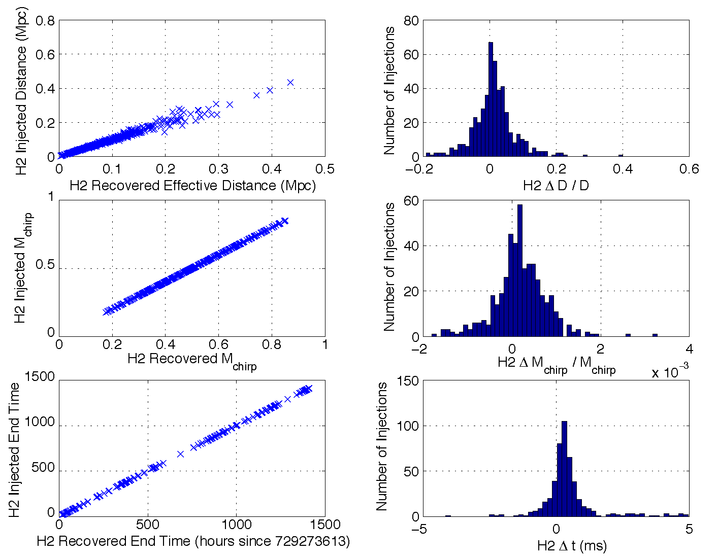
Figure 12: The panels in this figure compare the measured values of effective distance, chirp mass and end time with the known values for the injected waveforms in the Monte Carlo simulation in the H2 detector.

A comparison of the inspiral parameters recovered by the pipeline and the known injection parameters from signals injected in the Monte Carlo simulation are shown for L1, H1 and H2 in figures 10, 11 and 12 respectively. It can be seen that the effective distance recorded by the search code is unbiased in all cases, and can typically be recovered to an accuracy of $\sim 10\%$. This is comparable to the $10\%$ distance uncertainty to nearby galaxies. Using the measured coalescence phase, effective distance and difference in time of arrive at the two detectors, it is possible to gain information about the location of the signals, however a comprehensive study of this has not been performed for the S2 data. For all interferometers, the chirp mass is recovered extremely well with an accuracy of $0.1\%$. This consistent with the results quoted in [Cutler:1994] and is encouraging for the parameter measurement in the case of a detection. Although there appears to be a bias in the measure end time of the signal, this is due to the fact that the current implementation of the filtering code measures the end time of the template, not the coalescence time of the binary. The injected signals are generated with a time domain waveform generator[LAL] and recovered with the stationary phase waveforms described in chapter 4. There is a slight difference in the frequency at which these waveforms terminate: the time domain waveforms are terminated when the post-Newtonian phase evolution of equation (2.110) can no longer be evolved and the stationary phase waveforms are terminated when they reach the gravitational wave frequency of a test particle in the innermost stable circular orbit of Schwarzschild spacetime. As a result of this there is a small mass dependent offset between the end times of the waveform as recorded by the injection code and the filtering code. This will not affect the time coincidence test, however, as we demand that the templates have the same mass parameters in all the detectors. As a result this time offset will be identical between detectors and we can apply coincidence. Changes to the filtering code are planed to remove this offset in time measurement.

7.4 Background Estimation

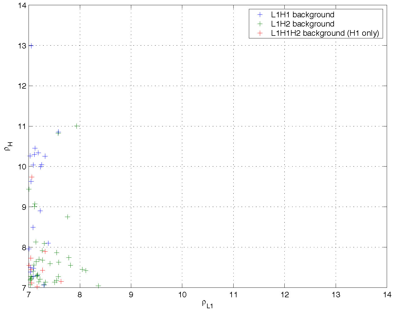
Figure 13: The signal-to-noise ratio of the background triggers produced by 20 time-slides. No triple coincident background triggers were observed. The colors are color coded depending on whether they were found in the triple, L1-H1 double of L1-H1 double triggers coincident data. No background triggers were found coincident in all three detectors, so the triggers from the triple coincident data set are from L1-H1 coincidence only.

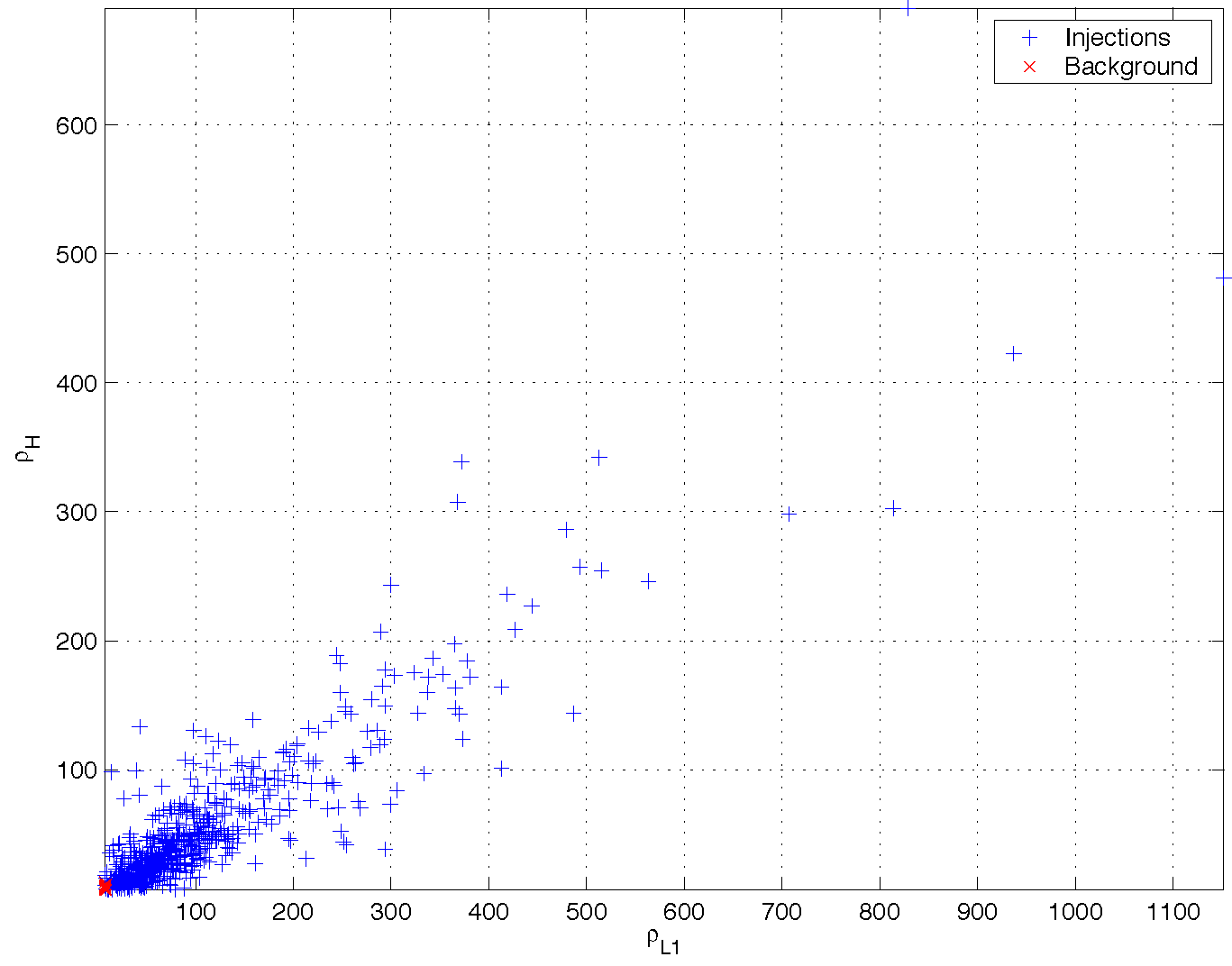
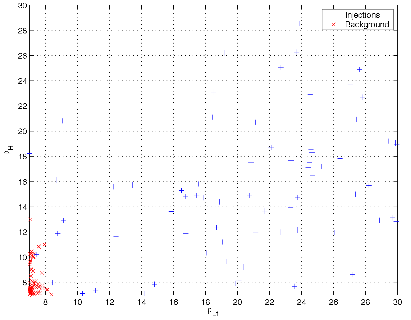
Figure 14: The plots in this figure compare the signal-to-noise ratios of the background triggers to those of the triggers corresponding to software injections from the Monte Carlo simulation. Notice in the upper plot that the signal-to-noise ratio of detected injections in L1 is a factor of $\sim 2$ higher than the signal-to-noise ratio in the LHO detectors, due to the greater sensitivity of L1. The lower plot shows a magnification of the low signal-to-noise ratio region. It can be seen that background triggers generally have a larger signal-to-noise ratio in the LHO detectors, suggesting the coherent statistic described in the text that gives greater weight to the L1 signal-to-noise ratio.

We estimate the background rate for this search by introducing an artificial time offset, or lag, $\Delta t$ in the triggers coming from the Livingston detector relative to the Hanford detector. The time-lag triggers are then fed into subsequent steps of the pipeline. The triggers that emerge from the end of the pipeline are considered a single trial representative of an output from a search if no signals are present in the data. By choosing a lag of more than 20 ms, we ensure that a true gravitational wave will not be coincident in the time-shifted data streams. We do not time-shift the two Hanford detectors relative to one another since there may be real correlations due to environmental disturbances. If the times of background triggers are not correlated at the sites, then the background rate can be measured. A total of 20 time-lags were analyzed to estimate the background. Note that the time lags use all the data and are not restricted to playground. The resulting distribution of time-lag triggers in the $(\rho_{\mathrm{H}},\rho_{\mathrm{L}})$ plane is shown in figure 13; the distribution of background triggers and injected signals are compared in figure 14. It can be seen that the signal-to-noise ratios of background triggers are higher in the LHO interferometers than in the L1 interferometer, whereas the signal-to-noise ratios of injections are louder in the L1 interferometer. This distribution suggested the form of a “coherent” signal-to-noise ratio $\hat{\rho}$ which gives a factor of 2 more significance to the signal-to-noise ratio in L1 compared to the signal-to-noise ratio in L1. Based on the studies of the background and injections, we chose a combined signal-to-noise statistic

$$\hat{\rho}^{2}=\rho^{2}_{\mathrm{L1}}+\frac{\rho_{\mathrm{H}}^{2}}{4}.$$ (7.2)

7.5 Upper Limit on BBHMACHO Inspiral in the S2 Playground Data

After the data quality cuts, discarding science segments with durations shorter than 2048 sec, and application of the instrumental veto in L1, a total of 35.2 hours of playground data remained; 22.0 hours of triple-detector data, 10.2 hours of L1-H1 and 3.97 hours of L1-H2. The analysis of the playground data produced no double or triple coincident inspiral candidates.

To determine an upper limit on the event rate we use the loudest event statistic[loudestGWDAW03] which uses the detection efficiency at the signal-to-noise ratio of the loudest trigger surviving the pipeline to determine an upper limit on the rate. If no triggers survive the pipeline, we use the signal-to-noise threshold as the loudest event. Suppose the population of sources produces Poisson-distributed events with a rate $\mathcal{R}$ per year per Milky Way Equivalent Galaxy (MWEG) and $N_{G}(\rho^{\ast})$ is the number of MWEGs to which the search is sensitive at $\rho\geq\rho^{\ast}$. Then the probability of observing an inspiral signal with $\rho>\rho^{\ast}$, given some rate $\mathcal{R}$ and some observation time $T$, is

$$P(\rho>\rho^{\ast};{\mathcal{R}})=1-e^{-{\mathcal{R}}TN_{G}(\rho^{\ast})}.$$ (7.3)

A trigger can arise from either an inspiral signal in the data or from background. If $P_{b}$ denotes the probability that all background triggers have signal-to-noise ratio less than $\rho^{\ast}$, then the probability of observing either an inspiral signal or a background trigger with $\rho>\rho^{\ast}$ is given by

$$P(\rho>\rho^{\ast};{\mathcal{R}},b)=1-P_{b}e^{-{\mathcal{R}}TN_{G}(\rho^{\ast})}.$$ (7.4)

Given the probability $P_{b}$, the total observation time $T$, and the number of Milky Way equivalent galaxies $N_{{G}}$ to which the search is sensitive, we find that the rate of binary black hole MACHO inspirals per MWEG is

$$\mathcal{R}_{90\%}=\frac{2.303+\ln P_{b}}{TN_{G}(\rho^{\ast})}$$ (7.5)

with 90% confidence. This is a frequentist upper limit on the rate. For ${\mathcal{R}}>{\mathcal{R}}_{90\%}$, there is more than $90\%$ probability that at least one event would be observed with SNR greater than $\rho_{\text{max}}$.

Since no coincident events were observed in the playground data, we determine the rate by measuring the efficiency of the pipeline at the (combined) signal-to-noise threshold

$$\hat{\rho}^{2}_{\mathrm{max}}=7^{2}+\frac{7^{2}}{4}=61.25.$$ (7.6)

This is a conservative limit on the rate. If we lowered the signal-to-noise thresholds until we observed the loudest trigger, then this trigger will have a signal-to-noise ratio less than the value given in equation (7.6); the measured efficiency will be greater than or equal to that used here so the rate will be less than or equal to which we quoted here. Furthermore, since we only have a small number of time lags, we neglect the background term $P_{b}$. Dropping this term will give a conservative value for upper limit[loudestGWDAW03].

If we restrict the mass parameters of the injected signals to those with a component in the range $0.15$ to $1.0\,M_{\odot}$, the mass range suggested by microlensing observations, we find that efficiency of the search pipeline at $\hat{\rho}^{\ast}=\sqrt{61.25}$ is

$$\varepsilon\left(\hat{\rho}^{\ast}=\sqrt{61.25}\right)=\frac{692}{756}=0.915.$$ (7.7)

The observation time for the playground data is $T=35.2\,\mathrm{hours}=4\times 10^{-3}\,\mathrm{yr}$ and so the upper limit on the rate of binary black hole MACHO inspirals in the playground data is

$$\mathcal{R}_{90\%}=\frac{2.303}{0.915\times 4\times 10^{-3}}=627\,\mathrm{yr}^{-1}\,\mathrm{MWEG}^{-1}.$$ (7.8)

The amount of non-playground data in the full S2 data, again discarding science segments with durations shorter than 2048 sec, and application of the instrumental veto in L1, there is a total of 345 hours of non-playground data; 225 hours of triple-detector data, 90 hours of L1-H1 and 30 hours of L1-H2. Assuming that the signal-to-noise ratio of the loudest event in the full data is comparable to $\hat{\rho}^{2}=61.25$, which is suggested by the background triggers, we may estimate the achievable upper limit as

$$\mathcal{R}_{90\%}=\frac{2.303}{0.915\times 3.9\times 10^{-2}}=64\,\mathrm{yr}^{-1}\,\mathrm{MWEG}^{-1}.$$ (7.9)

This upper limit is three orders of magnitude larger than the upper bound on the rate of $R=0.05\times 2^{\pm 1}\,\mathrm{yr}^{-1}\,\mathrm{MWEG}^{-1}$, so we are not yet able to constrain the fraction of the Galactic halo in BBHMACHOs. The sensitivity of the interferometers during the S2 search is roughly an order of magnitude from design sensitivity, however. For a $(0.5,0.5)\,M_{\odot}$ binary, at design sensitivity the interferometers will be sensitive to $\sim 50$ MWEG, so in one year of data taking, assuming no detections have been made, an upper limit on rate of BBHMACHO inspirals of $R=3\times 10^{-2}\,\mathrm{yr}^{-1}\,\mathrm{MWEG}^{-1}$ are possible (assuming $P_{b}=0.5$) which will significantly impact the theoretical rate estimates. Additionally, since the range of the search scales as a function of the mass, the possibility for detecting more massive BBHMACHO binaries increases as more galaxies become accessible and the rate can be further constrained.

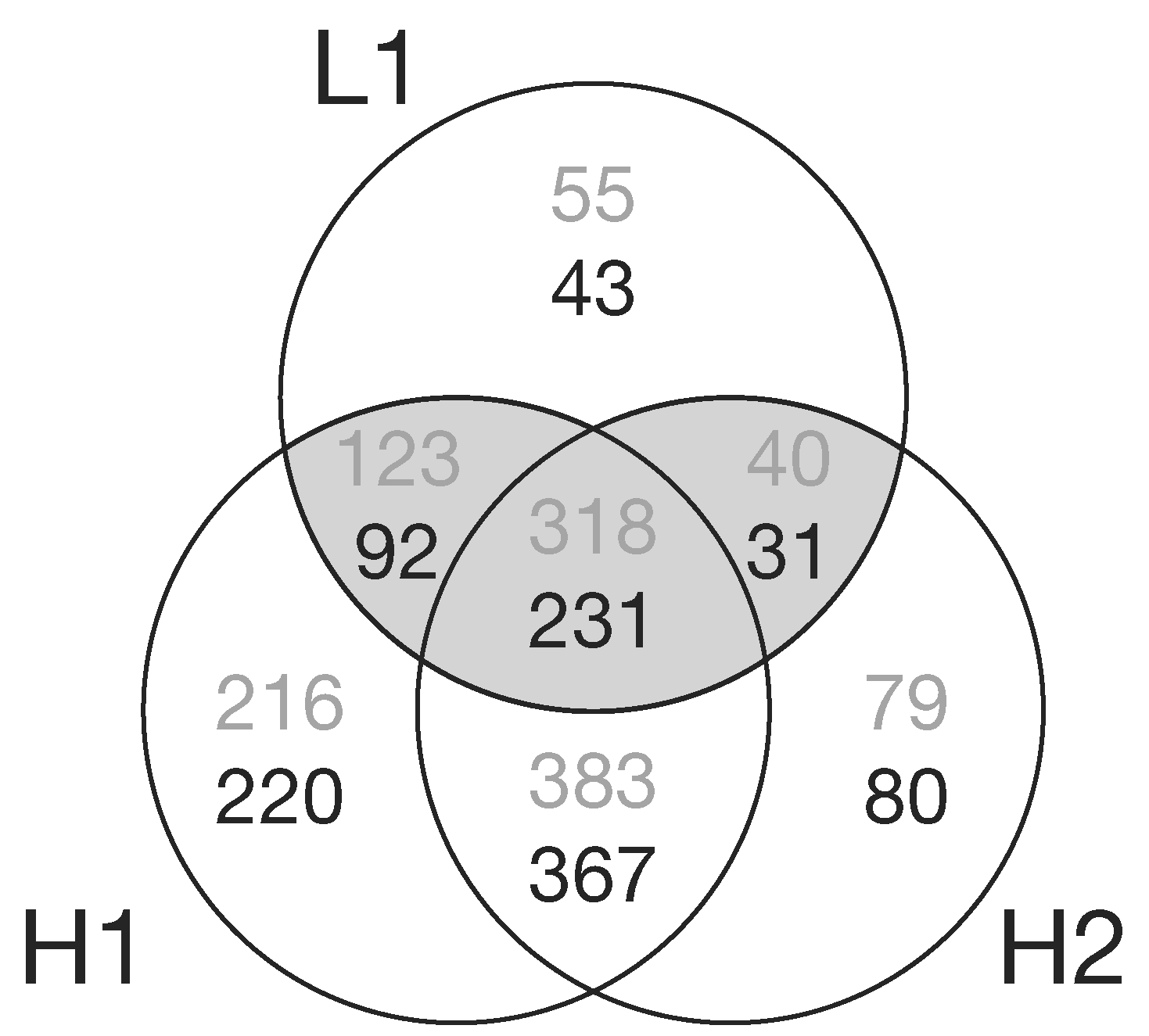
Figure 1: The Venn diagram shows the number of hours that each detector combination was operational during the S2 run. The upper number gives the amount of time the specific instruments were operational. The lower number gives the total non-playground time which was searched for inspiral triggers. The shaded region corresponds to the data used in the S2 MACHO search.

Parameter	Description	value
$f_{\mathrm{hp}}$	High Pass Filter Frequency	$100$ Hz
$O_{\mathrm{hp}}$	High Pass Filter Order	$100$ Hz
$f_{\mathrm{low}}$	Low Frequency Cutoff	$100$ Hz
$m_{\mathrm{min}}$	Template bank lower component mass	$0.2\,M_{\odot}$
$m_{\mathrm{max}}$	Template bank upper component mass	$1.0\,M_{\odot}$
$\mathbb{M}$	L1 template bank minimal match	0.95
$\rho^{\ast}_{\mathrm{L1}}$	L1 signal-to-noise ratio threshold	7.0
$\Xi^{\ast}_{\mathrm{L1}}$	L1 $\chi^{2}$ veto threshold	3.1
$\rho^{\ast}_{\mathrm{H1}}$	H1 signal-to-noise ratio threshold	7.0
$\Xi^{\ast}_{\mathrm{H1}}$	H1 $\chi^{2}$ veto threshold	5.0
$\rho^{\ast}_{\mathrm{H2}}$	H2 signal-to-noise ratio threshold	7.0
$\Xi^{\ast}_{\mathrm{H2}}$	H2 $\chi^{2}$ veto threshold	10.0
$p$	Number of bins in $\chi^{2}$ veto	15
$\delta^{2}$	$\chi^{2}$ veto mismatch parameter	0.2
$\delta m$	Trigger mass coincidence parameter	0.0
$\delta t_{\mathrm{HH}}$	H1-H2 trigger time coincidence parameter	0.001 s
$\delta t_{\mathrm{LH}}$	L1-H1, L1-H2 trigger time coincidence parameter	0.011 s
$\kappa_{HH}$	H1-H2 trigger amplitude coincidence parameter	0.5
$\kappa_{LH}$	L1-H1, L1-H2 trigger amplitude coincidence parameter	1000.0
$\epsilon$	Trigger amplitude coincidence parameter	2.0

Table 1: A complete list of the parameters that were selected at the various stages of the pipeline. These values are justified in the text.

Chapter 8 Conclusion

Although the upper limit that we have placed on the rate of binary black hole MACHO inspirals in the galaxy is lower than the upper bound of the predicted rates, the LIGO interferometers were not at design sensitivity when the S2 data was taken. At present, the sensitivities of the instruments are significantly better than during S2, as can be seen from figure 1, and progress on reducing noise in the interferometers continues apace. The increase in detector sensitivity makes a larger volume of the Universe accessible to searches for binary inspirals. In addition to this, the amount of data is also increasing as the interferometers become more stable.

These improvements in the instruments will increase the chance of detecting gravitational waves from binary inspirals. If the rates of binary black hole MACHO coalescence are truly as high as predicted, then initial LIGO would stand an excellent chance of detecting an inspiral. The first detection of gravitational waves will be a major scientific breakthrough and will yield and enormous amount of scientific information, particularly if the detection came from a binary black hole MACHO. The length of binary black hole MACHO inspirals in the sensitive band of the interferometer will allow extremely accurate parameter estimation as well as tests of post-Newtonian theory. For systems with total mass greater than $\sim 0.64\,\mathrm{M}_{\odot}$ LIGO will be sensitive to the coalescence of the binary and will be able to study the strong gravitational field effects when two binary black holes merge. When this is coupled with the accurate parameter estimation available from the earlier part of the waveform, the inspiral of a binary black hole MACHO could be an excellent laboratory for General Relativity. A detection would also impact the studies of halo dark matter and early universe physics, providing a MACHO component to the halo and suggesting that primordial black holes do indeed form in the universe.

In the absence of detection, the improvements in detector sensitivity will dramatically improve the upper limits placed on the rate of binary black hole MACHO inspirals. Once these rates are below the predicted rates, we may begin to use observations from gravitational wave interferometers to constrain the fraction of galactic halos in the form of primordial black hole MACHOs. While this may not be as significant as a detection, it will still be of interest to the astrophysical community.

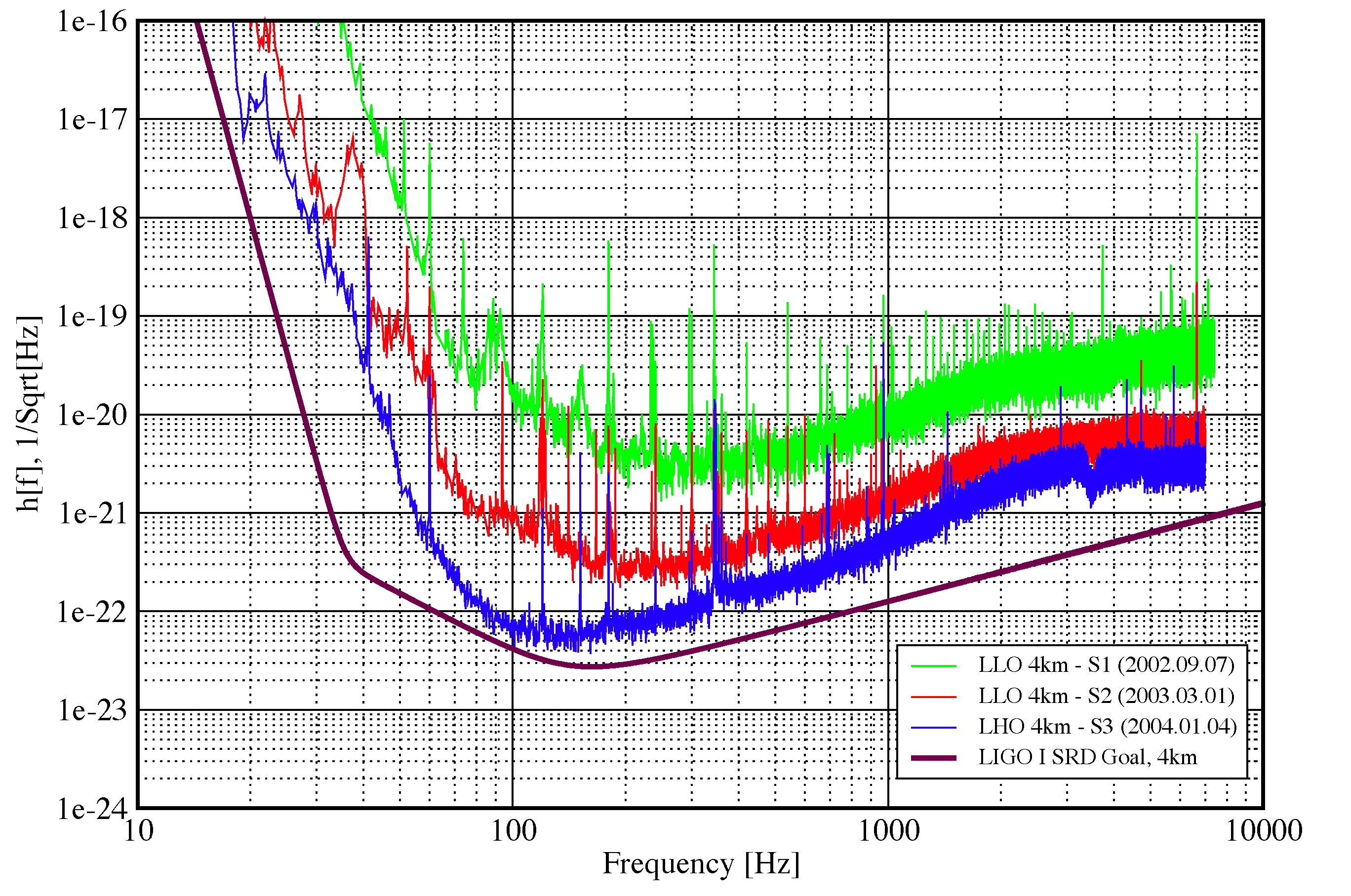
Figure 1: Comparison of the best sensitivities of the LIGO interferometers between science runs. The solid curve shows the design sensitivity for the $4$ km interferometers: the LHO $4$ km is only a factor of $\sim 2$ away from design at $100$ Hz during S3.

Curriculum Vitae

Title of Dissertation
	Searching for Gravitational Radiation from Binary Black Hole MACHOs
	in the Galactic Halo

Full Name
	Duncan A. Brown

Place and Date of Birth
	Nottingham, United Kingdom	January 25, 1976

Colleges and Universities,		Years attended and degrees
	University of Newcastle Upon Tyne		1994–1999,	M.Math.
	University of Wisconsin–Milwaukee		1999–2004,	Ph.D.

• 
  

Awards	and	Fellowships
		2003	UWM Chancellor’s Graduate Student Fellowship
2003	UWM Dissertator Fellowship
2002	Physics Graduate Student Trust Fund Award
2002	UWM Chancellor’s Graduate Student Fellowship
2002	UWM Graduate School Fellowship
2001	Papastamatiou Scholarship
1999	Institute of Mathematics and Its Applications Prize
1997	Stroud Book Prize for Theoretical Physics

	Major Department
Physics

          Professor Patrick Brady Date

Bibliography

- [1] A. Einstein. Approximative Integration of the Field Equations of Gravitation. Preuss. Akad. Weiss. Berlin, page 688, 1916.
- [2] F. A. E. Pirani. Acta Physica Polonica, 15:389, 1956.
- [3] G. F. Moss, L. R. Miller, and Forward R. L. Photon-noise-limited laser tranducer for gravitational antenna. Applied Optics, 10:2495–2498, 1971.
- [4] R Weiss. Electromagnetically coupled broadband gravitational wave antenna. Quarterly Progress Report of the Research Laboratory of Electronics of the Massachsetts Institutue of Technology, 105:54, April 1972.
- [5] R. P. Drever et al. A gravity-wave detector using optical cavity sensing. In E. Schmutzer, editor, Proceedings of the Ninth International Conference on General Relativity and Gravitation, pages 265–267. Cambridge University Press, Cambridge, UK, 1983.
- [6] Peter R. Saulson. Fundamentals of Interferometric Gravitational Wave Detectors. World Scientific, Singapore, 1994.
- [7] R. A. Hulse and J. H. Taylor. Discovery of a pulsar in a binary system. Astrophysical J., 195:L51–L53, January 1975.
- [8] J. H. Taylor and J. M. Weisberg. A new test of general relativity : gravitational radiation and the binary pulsar psr 1913 +16. 253:908, 1982.
- [9] J. H. Taylor and J. M. Weisberg. Further experimental tests of relativistic gravity using the binary pulsar 1913+16. 345:434, 1989.
- [10] E. S. Phinney. The rate of neutron star binary mergers in the universe: Minimal predictions for gravity wave detector. 380:L17, 1991.
- [11] B. C. Barish and R. Weiss. Ligo and the detection of gravitational waves. Phys. Today, 52 (Oct)(10):44–50, 1999.
- [12] B. Abbott et al. Analysis of ligo data for gravitational waves from binary neutron stars. Phys. Rev. D, 69(LIGO-P030024-00-R):122001, 2004.
- [13] Takashi Nakamura, Misao Sasaki, Takahiro Tanaka, and Kip S. Thorne. Gravitational waves from coalescing black hole macho binaries. 487:L139, 1997.
- [14] B. Abbott et al. Search for binary neutron star coalescence in the local group. (LIGO-P040024-01-Z), 2004. in preparation.
- [15] C W Misner, K S Thorne, and J A Wheeler. Gravitation. W.H. Freeman, New York, NY, 1973.
- [16] K. S. Thorne. The theory of gravitational radiation: An introductory review. In N. Deruelle and T. Piran, editors, Gravitational Radiation, pages 1–57. North Holland, Amsterdam, 1983.
- [17] R M Wald. General Relativity. University of Chicago Press, Chicago, IL, 1984.
- [18] F Acernese et al. The present status of the virgo central interferometer. 19:1421, 2002.
- [19] H. Lück and the GEO600 team. The GEO600 project. 14:1471, 1997.
- [20] Peter Fritschel, Rolf Bork, Gabriela González, Nergis Mavalvala, Dale Ouimette, Haisheng Rong, Daniel Sigg, and Michael Zucker. Readout and control of a power-recycled interferometric gravitational-wave antenna. 40:4988, 2001.
- [21] Rana Adhikari. Sensitivity and Noise Analysis of 4 km Laser Interferometric Gravitational Wave Antennae. PhD thesis, MIT, Cambridge, MA, 2004.
- [22] R. Adhikari, G. González, M. Landry, and B. O’Reilly. Class. Quant. Grav., 20:S903–S914, 2003.
- [23] B. F. Schutz and M. Tinto. Antenna patterns of interferometric detectors of gravitational waves. I - Linearly polarized waves. Mon. Not. Roy. Astr. Soc., 224:131–154, January 1987.
- [24] Luc Blanchet, Bala R. Iyer, Clifford M. Will, and Alan G. Wiseman. Gravitational wave forms from inspiralling compact binaries to second-post-newtonian order. 13:575, 1996.
- [25] J Mathews and R L Walker. Mathematical Methods of Physics. W. A. Benjamin, New York, NY, 1970.
- [26] Clifford M. Will and Alan G. Wiseman. Gravitational radiation from compact binary systems: Gravitational waveforms and energy loss to second post-newtonian order. 54:4813–4848, 1996.
- [27] Cutler C and Flanagan E. Gravitational waves from mergin compact binaries: How accurately can one extract the binary’s parameters from the inspiral waveform? 49:2658, 1994.
- [28] Serge Droz, Daniel J. Knapp, Eric Poisson, and Benjamin J. Owen. Gravitational waves from inspiraling compact binaries: Validity of the stationary-phase approximation to the fourier transform. Phys. Rev., D59:124016, 1999.
- [29] Kim Griest. Galactic microlensing as a method of detecting massive compact halo objects. Astrophys. J., 366:412–421, 1991.
- [30] Kim Griest. The nature of the dark matter. 1995.
- [31] R. Sancisi and T. S. van Albada. H I rotation curves of galaxies. In IAU Symp. 117: Dark matter in the universe, pages 67–80, 1987.
- [32] E. I. Gates, G. Gyuk, and M. S. Turner. The Local Halo Density. Astrophys. J., 449:L123+, August 1995.
- [33] H.-W. Rix. The Shapes of Dark Halos. In IAU Symp. 169: Unsolved Problems of the Milky Way, pages 23–29, 1996.
- [34] Steven Weinberg. A new light boson? Phys. Rev. Lett., 40:223–226, 1978.
- [35] Mark W. Goodman and Edward Witten. Detectability of certain dark-matter candidates. Phys. Rev., D31:3059, 1985.
- [36] E. J. Kerins and B. J. Carr. Infrared searches for dark matter in the form of brown dwarfs. Mon. Not. Roy. Astr. Soc., 266:775–+, February 1994.
- [37] Bohdan Paczynski. Gravitational microlensing by the galactic halo. Astrophys. J., 304:1–5, 1986.
- [38] S. Refsdal. The gravitational lens effect. Mon. Not. Roy. Astr. Soc., 128:295–+, 1964.
- [39] C. Alcock et al. The macho project: Microlensing results from 5.7 years of lmc observations. Astrophys. J., 542:281–307, 2000.
- [40] C. Afonso et al. Limits on galactic dark matter with 5 years of eros smc data. Astron. Astrophys., 400:951–956, 2003.
- [41] C. Alcock, R. A. Allsman, D. Alves, T. S. Axelrod, A. C. Becker, D. P. Bennett, K. H. Cook, K. C. Freeman, K. Griest, J. Guern, M. J. Lehner, S. L. Marshall, B. A. Peterson, M. R. Pratt, P. J. Quinn, A. W. Rodgers, C. W. Stubbs, W. Sutherland, and D. L. Welch. The MACHO Project LMC Microlensing Results from the First Two Years and the Nature of the Galactic Dark Halo. ArXiv Astrophysics e-prints, June 1996.
- [42] C. Alcock et al. The macho project first year lmc results: The microlensing rate and the nature of the galactic dark halo. Astrophys. J., 461:84, 1996.
- [43] David S. Graff and Katherine Freese. Analysis of a hubble space telescope search for red dwarfs: Limits on baryonic matter in the galactic halo. 1995.
- [44] David S. Graff and Katherine Freese. The mass-function of low mass halo stars: Limits on baryonic halo dark matter. Astrophys. J., 467:L65, 1996.
- [45] B. Goldman, C. Afonso, C. Alard, J.-N. Albert, A. Amadon, J. Andersen, R. Ansari, É. Aubourg, P. Bareyre, F. Bauer, J.-P. Beaulieu, G. Blanc, A. Bouquet, S. Char, X. Charlot, F. Couchot, C. Coutures, F. Derue, R. Ferlet, P. Fouqué, J.-F. Glicenstein, A. Gould, D. Graff, M. Gros, J. Haissinski, C. Hamadache, J.-C. Hamilton, D. Hardin, J. de Kat, A. Kim, T. Lasserre, L. Le Guillou, É. Lesquoy, C. Loup, C. Magneville, B. Mansoux, J.-B. Marquette, É. Maurice, A. Maury, A. Milsztajn, M. Moniez, N. Palanque-Delabrouille, O. Perdereau, L. Prévot, N. Regnault, J. Rich, M. Spiro, P. Tisserand, A. Vidal-Madjar, L. Vigroux, S. Zylberajch, and The EROS collaboration. EROS 2 proper motion survey: Constraints on the halo white dwarfs. Astron. and Astrophys., 389:L69–L73, July 2002.
- [46] C. A. Nelson, K. H. Cook, T. S. Axelrod, J. R. Mould, and C. Alcock. A Proper-Motion Survey for White Dwarfs with the Wide Field Planetary Camera 2. Astrophysical J., 573:644–661, July 2002.
- [47] Michel Creze et al. Dark halo baryons not in ancient halo white dwarfs. 2004.
- [48] T. Nakamura, Y. Kan-Ya, and R. Nishi. The Minimum Total Mass of MACHOs and Halo Models of the Galaxy. Astrophysical J., 473:L99+, December 1996.
- [49] P. Salati, R. Taillet, E. Aubourg, N. Palanque-Delabrouille, and M. Spiro. Kinematics of lmc stellar populations and self-lensing optical depth. 1999.
- [50] N. Wyn Evans, Geza Gyuk, Michael S. Turner, and James Binney. The lmc microlensing events: Evidence for a warped and flaring milky way disk? Astrophys. J., 501:L45, 1998.
- [51] Lee Samuel Finn. Gravitational radiation sources for acoustic detectors. 1996.
- [52] Y. B. Zel’Dovich and I. D. Novikov. The Hypothesis of Cores Retarded during Expansion and the Hot Cosmological Model. Soviet Astronomy, 10:602–+, February 1967.
- [53] B. J. Carr and S. W. Hawking. Black holes in the early Universe. Mon. Not. Roy. Astr. Soc., 168:399–416, August 1974.
- [54] Junichi Yokoyama. Formation of macho-primordial black holes in inflationary cosmology. Astron. Astrophys., 318:673, 1997.
- [55] J. Yokoyama. Formation of primordial black holes in inflationary cosmology. Prog. Theor. Phys. Suppl., 136:338–352, 1999.
- [56] Karsten Jedamzik. Primordial black hole formation during the qcd epoch. Phys. Rev., D55:5871–5875, 1997.
- [57] P. C. Peters. Gravitational radiation and the motion of two point masses. 136:B1224, 1964.
- [58] Kunihito Ioka, Takeshi Chiba, Takahiro Tanaka, and Takashi Nakamura. Black hole binary formation in the expanding universe: Three body problem approximation. Phys. Rev., D58:063003, 1998.
- [59] V. Kalogera et al. The cosmic coalescence rates for double neutron star binaries. apj, 601:L179–L182, 2004.
- [60] K. G. Begeman. H I rotation curves of spiral galaxies. I - NGC 3198. Astron. and Astrophys., 223:47–60, October 1989.
- [61] L A Wainstein and V D Zubakov. Extraction of signals from noise. Prentice-Hall, Englewood Cliffs, NJ, 1962.
- [62] Lee S. Finn. Detection, measurement and gravitational radiation. Phys. Rev., D46:5236–5249, 1992.
- [63] Lee Samuel Finn and David F. Chernoff. Observing binary inspiral in gravitational radiation: One interferometer. Phys. Rev., D47:2198–2219, 1993.
- [64] C W Helstrom. Elements of Signal Detection and Estimation. Prentice-Hall, Englewood Cliffs, NJ, 1995.
- [65] W H Press, S A Teukolsky, W T Vetterling, and B P Flannery. Numerical Recipies in C. Cambridge, Cambridge, UK, 1992.
- [66] S. B. Anderson, W. G. Anderson, J. K. Blackburn, P. R. Brady, D. A. Brown, P. Charlton, J. D. E. Creighton, T. D. Creighton, L. S. Finn, J. D. Romano, D. Sigg, J. T. Whelan, A. G. Wiseman, and J. Zweizig. Conventions for data and software products of the ligo and the lsc. Technical Report LIGO-T010095-00-D, LIGO Project, 2001.
- [67] Bruce Allen. A time-frequency discriminator for gravitational wave detection. 2004.
- [68] P. D. Welch. The use of fast fourier transform for the estimation of power spectra: A method based on time averaging over short, modified periodograms. IEEE Trans. Audio Electroacoust., 15:70–73, 1967.
- [69] Bruce Allen. grasp: a data analysis package for gravitational wave detection, version 1.9.8, May 2000. pages 180-188.
- [70] Matt Evans. Lock Aquisition in Resonant Optical Interferometers. PhD thesis, Caltech, Pasadena, CA, 2004.
- [71] Todd Tannenbaum, Derek Wright, Karen Miller, and Miron Livny. Condor – a distributed job scheduler. In Thomas Sterling, editor, Beowulf Cluster Computing with Linux. MIT Press, October 2001.
- [72] Benjamin J. Owen and B. S. Sathyaprakash. Matched filtering of gravitational waves from inspiraling compact binaries: Computational cost and template placement. 60:022002, 1999.
- [73] M. Ito. glitchmon: A DMT monitor to look for transient signals in selected channels. Developed using the LIGO Data Monitoring Tool (DMT) library.
- [74] B. Abbott et al. Detector description and performance for the first coincidence observations between ligo and geo. Nucl. Instrum. Methods, A517(LIGO-P030024-00-R):154–179, 2004.
- [75] Bruce Allen. Ligo calibration accuracy. Technical Report LIGO-T960189-00-Z, LIGO Project, 1996.
- [76] B. Abbott et al. An upper limit on the rate of binary black hole macho inspiral in the galactic halo. 2004. In Preparation.
- [77] LSC Algorithm Library software packages lal and lalapps. The CVS tag version macho_2004061801 of lal, and macho_2004061801 of lalapps were used in this analysis.
- [78] P. Brady, J. Creighton, and A. Wiseman. Upper limits on gravitational-wave signals based on loudest events. 2004. to appear in Class. Quant. Grav.