Wakes in a Collisional Quark-Gluon Plasma

Abstract

Wakes created by a parton moving through a static and infinitely extended quark-gluon plasma are considered. In contrast to former investigations collisions within the quark-gluon plasma are taken into account using a transport theoretical approach (Boltzmann equation) with a Bhatnagar-Gross-Krook (BGK) collision term. Within this model it is shown that the wake structure changes significantly compared to the collisionless case.

In ultrarelativistic heavy-ion experiments (SPS, RHIC) indications have been found for a temporary formation of a strongly coupled quark-gluon plasma (QGP) phase in the fireball created in nucleus-nucleus collisions (see e.g. Ref.Ullrich2007 ). The main problem of this programme is to find clear signatures for the presence of a short-living QGP phase in this fireball. One promising class of signatures are hard probes, in particular high-energy partons of a few GeV or more, i.e. with an energy much higher than the temperature of the QGP. Energetic partons with a large transverse momentum, produced in initial hard parton collisions before the formation of an equilibrated fireball, propagate through the fireball. In this process they will lose energy, which depends on the state of the fireball (QPG or hadronic matter). Energetic partons manifest themselves at jets arriving in the detectors. The amount of jet quenching due to the propagation of the leading parton of the jet through the fireball can therefore serve as a signature for the QGP formation Pluemer1990 ; Baier2000 . A strong jet quenching and suppression of high $p_{T}$ hadron spectra have been observed at RHIC indicating the presence of a QGP phase RHIC . Another phenomenon related to the propagation of a high-energy parton through the QGP are wakes and Mach cones which may be observable as conical flow and shock waves in particle correlations Stoecker2005 ; Ruppert2005 ; Satarov2005 ; Shuryak2006 ; Chakraborty2006 ; remark1 .

In electromagnetic plasmas wakes are a well known phenomena. Theoretically they can be investigated by considering transport equations. In the collisionless case they follow from the dielectric functions by solving the Vlasov equation together with the Poisson equation. It has been shown in this way that wakes are also created in a QGP, leading eventually to attractive potentials and Mach cones as well known in plasma physics (see below). Attractive potentials between partons might lead to bound states and may modify the $J/\psi$ suppression pattern Chakraborty2006 . In the static case, i.e. for a parton at rest, the wake potential reduces to the usual Yukawa potential describing Debye screening Mustafa2005 .

Here we want to extend these investigations by taking into account collisions in the QGP. For this purpose we start from the Boltzmann equation approximating the collision term by the BGK description Bhatnagar1954 , allowing an analytic expression for the dielectric functions Carrington2004 ; remark2 . In this approach the collision term is replaced by a momentum independent collision rate which we take as a parameter. This model has been used to study dispersion relations Carrington2004 and instabilities Schenke2006 in a collisional QGP. Whereas the changes in the case of the dispersion relations are marginal - however the longitudinal plasma modes cross the light cone in a collisional plasma -, instabilities can be suppressed efficiently due to collisions. In the case of complex plasmas, i.e., low-temperature discharge plasmas with microparticles such as dust grains Fortov2005 , wake potentials due to ion flow, leading to an attractive force between the negatively charged microparticles, are investigated intensively (see e.g. Bashkirov2004 ). Also collisions between the ions and the neutral gas have been taken into account in this case and have been shown to truncate the wakes effectively Lampe2000 . In general the collisions modify the wake potential by decelerating the ions. Therefore the positive ion cloud, responsible for the attractive part of the wake potential, is concentrated nearer to the dust grain, causing a narrower but deeper potential well.

The longitudinal and transverse dielectric functions of a collisional QGP within the BGK approach are given by Carrington2004 ,

$$\epsilon_{l}\left(\omega,k\right) = 1+\frac{m_{D}^{2}}{k^{2}}\left(1-\frac{\omega+i\nu}{2k}\ln{\frac{\omega+i\nu+k}{\omega+i\nu-k}}\right)\left(1-\frac{i\nu}{2k}\ln{\frac{\omega+i\nu+k}{\omega+i\nu-k}}\right)^{-1}$$

$$\epsilon_{t}\left(\omega,k\right) = 1-\frac{m_{D}^{2}}{2\omega\left(\omega+i\nu\right)}\left\{1+\left[\frac{\left(\omega+i\nu\right)^{2}}{k^{2}}-1\right]\left(1-\frac{\omega+i\nu}{2k}\ln{\frac{\omega+i\nu+k}{\omega+i\nu-k}}\right)\right\}\,,$$ (1)

where $\nu$ is the collision rate and $m_{D}=\sqrt{1+n_{f}/6}\,gT$ the Debye screening mass. Here $n_{f}$ is the number of quark flavors in the QGP. From the dielectric functions the dispersion relations follow Carrington2004 , e.g. the longitudinal mode (plasmon) from $\epsilon_{l}(\omega,k)=0$. Note that $\omega$ has a real and imaginary part here.

The induced charge density by a parton with color charge $Q^{a}$ propagating through the QGP with velocity $v$ follows from Chakraborty2006

$$\rho^{a}_{\rm{ind}}(t,{\vec{\mathbf{r}}})=2\pi Q^{a}\ \int\frac{d^{3}k}{(2\pi)^{3}}\int\frac{d\omega}{2\pi}\exp\left[i\left({\vec{k}}\cdot{\vec{r}}-\omega t\right)\right]\left[\frac{1}{\epsilon_{l}(\omega,k)}-1\right]\ \delta(\omega-{\vec{k}}\cdot{\vec{v}})\,\,.$$ (2)

Due to the delta function $\omega$ is restricted here to real values and is always in the space-like region for $0<v<1$.

The induced charge density using cylindrical coordinates can be written as remark3

$$\rho^{a}_{\rm{ind}}(\rho,z,t) = \frac{Q^{a}}{2\pi^{2}v}\int_{0}^{\infty}d\kappa\,\kappa\,J_{0}(\kappa\rho)\int_{0}^{\infty}\ d\omega\,\Biggl{\{}\cos\left[\omega\left(\frac{z}{v}-t\right)\ \right]\left(\frac{{\rm Re}\,\epsilon_{l}}{\Delta}-1\right)$$ (3)

$$+ \sin\left[\omega\left(\frac{z}{v}-t\right)\right]\frac{{\rm Im}\,\epsilon_{l}}{\Delta}\Biggr{\}}\,\,,$$

where $J_{0}$ is the Bessel function, $\Delta=[{\rm Re}\,\epsilon_{l}]^{2}+[{\rm Im}\,\epsilon_{l}]^{2}$, and $\kappa=\sqrt{k^{2}-{\omega^{2}}/{v^{2}}}$.

The real and imaginary parts of the dielectric functions read

$${\rm Re}\,\epsilon_{l} = 1+\frac{m_{D}^{2}}{4k^{4}f\left(\omega,k,\nu\right)}\left[4k^{2}+\nu^{2}\left(\theta^{2}+\ln^{2}{R}\right)-2k\left(\omega\ln{R}+2\nu\theta\right)\right]\,,$$

$${\rm Im}\,\epsilon_{l} = \frac{m_{D}^{2}\omega}{4k^{4}f\left(\omega,k,\nu\right)}\left[2k\theta-\nu\left(\ln^{2}{R}+\theta^{2}\right)\right]\,,$$

where

$$R = \frac{\sqrt{\left(\omega^{2}-k^{2}+\nu^{2}\right)^{2}+4k^{2}\nu^{2}}}{\left(\omega-k\right)^{2}+\nu^{2}}\,,$$

$$\theta = \arccos\frac{\omega^{2}-k^{2}+\nu^{2}}{\sqrt{\left(\omega^{2}-k^{2}+\nu^{2}\right)^{2}+4k^{2}\nu^{2}}}\,,$$ (4)

and

$$f\left(\omega,k,\nu\right) = \left(1-\frac{\nu\theta}{2k}\right)^{2}+\frac{\nu^{2}\ln^{2}{R}}{4k^{2}}\,.$$ (5)

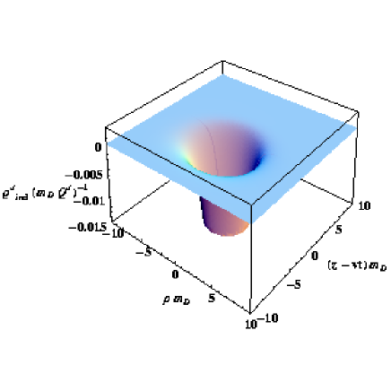
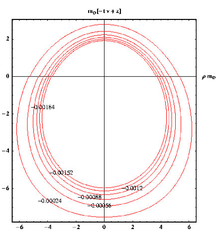
Figure 1: Left panel: Spatial distribution of the induced charge density for a parton moving with velocity $v=.55c$ with collisions for $(\nu=0,\,\,0.2m_{D},\,\,0.5m_{D},0.8m_{D})$ (Top to Bottom). Right panel: These plots show the corresponding contour plots

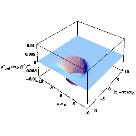
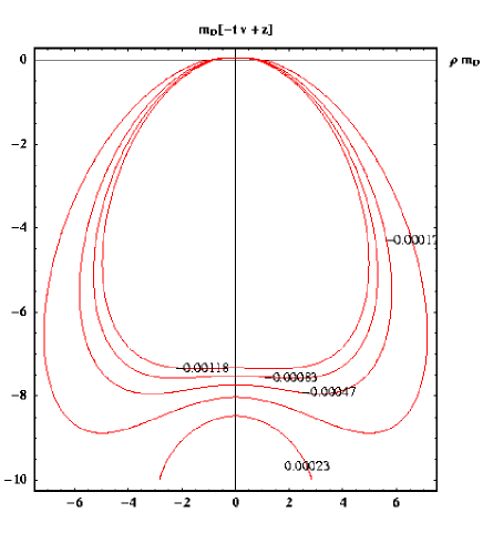
Figure 2: Left panel: Spatial distribution of the induced charge density for a parton moving with velocity $v=.99c$ with collisions for $(\nu=0,\,\,0.2m_{D},\,\,0.5m_{D},0.8m_{D})$ (Top to Bottom). Right panel: These plots show the corresponding contour plots

Solving (3) together with (5) numerically remark4 leads to the induced charge densities shown in Figs.1 and 2. The induced densities are proportional to $m_{D}^{3}$ and are scaled with $m_{D}$ as well as with the color charge $Q^{a}$ of the moving parton. Assuming for example $n_{f}=2$, $g=2$ (corresponding to $\alpha_{s}=1/\pi$), and $T=250$ MeV, we get a typical value of $m_{D}=580$ MeV. In Fig.1 the parton velocity is $v=0.55\>c$ and $v=0.99\>c$ in Fig.2. The left panels show the 3 dimensional plots for the choice $\nu=0$ to $\nu=0.8m_{D}$ remark5 . The right panels show the contour plots of the induced charge density. One observes a clear modification of the induced charge density due to the collision rate. The general structure of the wakes, corresponding to a modified screening, a cone-like structure, and wave excitation has been discussed in detail in Ref.Chakraborty2006 in the collisionless case. However, in the case of collisions these structures are smeared out and less pronounced for increasing $\nu$. We interpret this as the fact that the collisions, leading to thermalization, reduce the anisotropy caused by the perturbation of the moving charge in the QGP.

The wake potential is given by (see appendix)

$$\Phi^{a}({\vec{r}},t;{\vec{v}})=\frac{Q^{a}}{2\pi^{2}}\int d^{3}k\frac{e^{-i{\vec{k}}\cdot({\vec{r}}-{\vec{v}}t)}}{k^{2}\epsilon_{l}(\omega={\vec{v}}\cdot{\vec{k}},k)}.$$ (6)

It is of the same form as in the collisionless case, where it can be shown that in cylindrical coordinates it reduces to Chakraborty2006

$$\Phi^{a}\left(\rho,z,t\right) = \frac{2Q^{a}}{\pi v}\int_{0}^{\infty}d\kappa\,\kappa\,J_{0}\left(\kappa\rho\right)\int_{0}^{\infty}\,d\omega\frac{1}{k^{2}\Delta}\Biggl{\{}\cos\left[{\omega\left(\frac{z}{v}-t\right)}\right]\,{\rm{Re}}\,\epsilon_{l}$$ (7)

$$+\sin\left[\omega\left(\frac{z}{v}-t\right)\right]\,{\rm{Im}}\,\epsilon_{l}\Biggr{\}}\,.$$

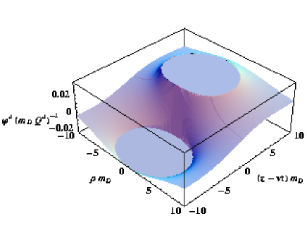
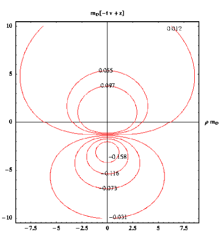
Figure 4: Left panel: Spatial distribution of the scaled wake potentials for a parton moving with velocity $v=.99c$ with collisions for $(\nu=0,\,\,0.2m_{D},\,\,0.5m_{D},\,\,0.8m_{D}$ (top to bottom panel). Right panel: These plots show the corresponding equipotential lines.

In Figs.3 and 4 the wake potentials scaled with respect to $m_{D}$ are shown for a parton with a given color charge $Q^{a}$ for velocities $v=0.55\>c$ and $v=0.99\>c$ and various values for the collision rate from $\nu=0$ to $\nu=0.8m_{D}$. It can be seen that collisions modify the strength and the structure of the wake potential significantly. Again, as in the case of the induced charge density the potential structure is washed out due to the collisions between the partons in the QGP. However, the potential becomes also stronger at finite collision rates, indicating that collisions in the QGP can enhance the attractive and repulsive parts of the interaction potential of a fast parton as in the case of non-relativistic plasmas. In particular, the attractive part behind the particle becomes deeper which might lead to an even stronger binding of diquark states propagating through the QGP as discussed in Ref.Chakraborty2006 . (Note that the induced charge density and wake potential diverge for point-like particles at the origin as in the static case corresponding to a Yukawa potential.)

In conclusion, we have applied the BGK approach in order to study the influence of collisions on the wake formation in the QGP. Clearly, this approach allows only qualitative statements. A consistent QCD approach, in which for example the collision rate are momentum dependent, is beyond the scope of this work. Keeping this in mind, we regard the (momentum independent) collision rate in our model as a free parameter. Anyway, our model demonstrates clearly that collisions in the QGP lead to a significant modification of wakes created by fast partons compared to the collisionless case. In particular, the wake structure is less pronounced. Hence possible observable effects such as the conical flow and wave excitations will be reduced. On the other hand, the attractive potential well becomes deeper. Similar effects of collisions have been observed in electromagnetic plasmas.

Acknowledgments We would like to thank M. Strickland for helpful discussions. M.H.T. would like to thank A. Ivlev for information on wakes in complex plasmas. MGM and RR are also thankful to S. Mallik for useful discussions.

I Appendix

Here we will explicitly derive equation (6) for the wake potential in the case of collisions. For the collisionless case it follows from a combination of the linearized Vlasov equation and the Poisson equation. Here we start from the kinetic equation with a BGK-collision term. The derivation from the equilibrium distribution function $f_{0}(p)$ is then given by (see (14) in Ref.Carrington2004 )

$$\delta f(\vec{p},\vec{r},t)=\left[-iq\vec{E}\cdot\frac{\partial f_{0}(p)}{\partial\vec{p}}+i\nu\eta f_{0}(p)\right]D^{-1},$$ (8)

where $q$ is the charge of the plasma particles and $D:=\omega+i\nu-\vec{k}\cdot\vec{v}$ with $\vec{v}={\vec{p}}/p$ in the ultrarelativistic case ($v=1$).

The quantity $\eta$ is given by

$$\eta=\frac{-iq}{N_{0}}\int dp\,\frac{(\vec{E}\cdot\vec{p})}{p}\frac{\partial f_{0}(p)}{\partial p}D^{-1}\left[1-\frac{i\nu}{N_{0}}\int dp\,f_{0}(p)D^{-1}\right]^{-1}$$ (9)

with the equilibrium particle number density $N_{0}$ and $dp=d^{3}p/(2\pi)^{3}$.

The Poisson equation for the potential $\Phi$ of a point charge $Q$ with velocity $\vec{v}$, where we drop the color index $a$ for convenience, in the plasma reads

$$\Delta\Phi({\vec{r}},t;{\vec{v}})=-4\pi Q\,\delta({\vec{r}}-{\vec{v}}t)-\rho({\vec{r}},t),$$ (10)

where $\rho=q\int dp\,\delta f$ is the induced charge density in the plasma. In momentum space it reads

$$k^{2}\Phi(\omega,{\vec{k}},{\vec{p}})=8\pi^{2}Q\,\delta(\omega-{\vec{v}}\cdot{\vec{k}})+q\int dp\,\delta f(\omega,{\vec{k}},{\vec{p}}).$$ (11)

Using ${\vec{E}}=-i{\vec{k}}\Phi$ in momentum space and $\partial f_{0}(p)/\partial{\vec{p}}={\vec{v}}\partial f_{0}(p)/\partial p$ we can write the Poisson equation by combining (11) with (8) and (9) as

$$k^{2}\Phi(\omega,{\vec{k}},{\vec{p}})=8\pi^{2}Q\,\delta(\omega-{\vec{v}}\cdot{\vec{k}})+k^{2}(1-\chi)\Phi,$$ (12)

where

$$\chi(\omega,k)=1+\frac{q^{2}}{k^{2}}\int dp\,(\vec{v}\cdot\vec{k})\frac{\partial f_{0}}{\partial p}D^{-1}-\frac{i\nu q\eta}{k^{2}\Phi}\int dp\,f_{0}D^{-1}.$$ (13)

Solving (12) for $\Phi$ and Fourier transforming it we obtain the wake potential

$$\Phi({\vec{r}},t;{\vec{v}})=\frac{Q}{2\pi^{2}}\int d^{3}k\,\frac{e^{-i{\vec{k}}({\vec{r}}-{\vec{v}}t)}}{k^{2}\chi(\omega={\vec{v}}\cdot{\vec{k}})}.$$ (14)

Comparing $\chi$ with the longitudinal dielectric function in the BGK approximation (see (17) and (18) in Carrington2004 ),

$$\epsilon_{l}(\omega,k) =1+\frac{q^{2}}{\omega k^{2}}\int dp\,(\vec{v}\cdot\vec{k})^{2}\frac{\partial f_{0}}{\partial p}D^{-1}-\frac{i\nu q\eta}{\omega k^{2}\Phi}\int dp\,(\vec{v}\cdot\vec{k})f_{0}D^{-1}$$ (15)

we find $\chi(\omega={\vec{v}}\cdot{\vec{k}})=\epsilon_{l}(\omega={\vec{v}}\cdot{\vec{k}})$. Hence (14) coincides with (6) and has the same form as in the collisionless case Chakraborty2006 .

This result can also be derived more generally, i.e. in an homogeneous and isotropic plasma with and without collisions, assuming linear response theory for the induced charge density Chakraborty2006 , $\rho_{ind}=(1/\epsilon_{l}-1)\rho_{ext}$, where the total charge density $\rho_{tot}=\rho_{ext}+\rho_{ind}$, and using the Poisson equation $\Phi=4\pi\rho_{ext}/(k^{2}\epsilon_{l})$ with $\rho_{ext}=2\pi Q\delta(\omega-{\vec{v}}\cdot{\vec{k}})$ after Fourier transformation.

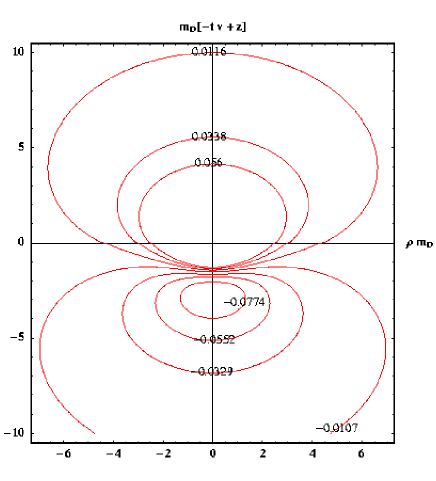
Figure 3: Left panel: Spatial distribution of the scaled wake potentials for a parton moving with velocity $v=.55c$ with collisions for $(\nu=0,\,\,0.2m_{D},\,\,0.5m_{D},\,\,0.8m_{D}$ (top to bottom panel). Right panel: These plots show the corresponding equipotential lines.

References

- (1) Ullrich T 2007 Nucl. Phys. A 783 1c
- (2) Plümer M and Gyulassy M 1990 Phys. Lett. B 243 342
- (3) Baier R, Schiff D, Zakharov B G 2000 Ann. Rev. Nucl. Part. Sci. 50 37
- (4) Adams et al. 2003 Phys. Rev. Lett. 91 172302; Adler S S et al. 2006 Phys. Rev. Lett. 96 202301
- (5) Stöcker H 2005 Nucl. Phys. A 750 121
- (6) Ruppert J and Müller B 2005 Phys. Lett. B 618 123
- (7) Satarov L M, Stöcker H, Mishustin I N 2005 Phys.Lett. B 627 64
- (8) Casalderrey-Solana J, Shuryak E V, Teaney D 2006 Nucl.Phys. A 774 577
- (9) Chakraborty P, Mustafa M G and Thoma M H 2006 Phys. Rev. D 74 094002
- (10) The wakes discussed here are associated with the collisional energy loss only not with the radiative Baier2000 . However, the latter might also produce a large-angle radiation of gluons in addition to the one by Mach cones Vitev2005 .
- (11) Vitev I (2005) Phys. Lett. B 630 78.
- (12) Mustafa M G, Thoma M H and Chakraborty P 2005 Phys. Rev. C 71 017901
- (13) Bhatnagar P L, Gross E P and Krook M 1954 Phys. Rev. 94 511
- (14) Carrington M E, Fugleberg T, Pickering D and Thoma M H 2004 Can. J. Phys. 82 671
- (15) In Ref.Carrington2004 the BGK-approach has been derived for the QED case. However, since the Vlasov aproach for QED and QCD is the same (apart from color and flavor factors), this approach can be used also for QCD at least as a model for taking collisions into account (see also Ref.Schenke2006 ).
- (16) Schenke B, Strickland M, Greiner C and Thoma M H 2006, Phys. Rev. D 73 125004
- (17) Fortov V E, Ivlev A V, Khrapak S A, Khrapak A G and Morfill G E 2005 Phys. Rep 421 1
- (18) Bashkirov A G 2004 Phys. Rev. E 69 046410
- (19) Lampe M, Joyce G, Ganguli G, and Gavrishchaka V 2000 Phys. Plasmas 7 3851
- (20) A typographical error in the factor in eq.(35) of Ref. Chakraborty2006 is now corrected here as .
- (21) We restrict to the physical Riemann sheet, i.e. with .
- (22) The collision rate in the QGP is momentum dependent and of the order of for color and for momentum exchange Thoma1994 . However, since is of the order of one in realistic situations, the choice of between 0 and is reasonable.
- (23) Thoma M H 1994 Phys. Rev. D 49 451