The dynamical status of the galaxy cluster Abell 115

Abstract

Aims. We present the results of a new spectroscopic and photometric survey of the hot, binary X–ray cluster A115 at $z=0.193$, containing a radio relic.

Methods. Our analysis is based on new spectroscopic data obtained at the Telescopio Nazionale Galileo for 115 galaxies and on new photometric data obtained at the Isaac Newton Telescope in a large field. We combine galaxy velocity and position information to select 85 galaxies recognized as cluster members, determine global dynamical properties and detect substructures.

Results. We find that A115 appears as a well isolated peak in the redshift space, with a global line–of–sight (LOS) velocity dispersion $\sigma_{\rm v}=1362_{-108}^{+126}$ km s^-1. Our analysis confirms the presence of two structures of cluster–type well recognizable in the plane of the sky and shows that they differ of $\sim 2000$ km s${}^{-1}\;$in the LOS velocity. The northern, high velocity subcluster (A115N) is likely centred on the second brightest cluster galaxy (BCM–A, coincident with radio source 3C28) and the northern X–ray peak. The southern, low velocity subcluster (A115S) is likely centred on the first brightest cluster galaxy (BCM–B) and the southern X–ray peak. We estimate that A115S is slightly dynamically more important than A115N having $\sigma_{\rm v}=900-1100$ km s${}^{-1}\;$vs. $\sigma_{\rm v}=750-850$ km s^-1. Moreover, we find evidence for two small groups at low velocities. We estimate a global cluster virial mass of 2.2–3.5 $\times 10^{15}\;h_{70}^{-1}\;M_{\odot}$.

Conclusions. Our results agree with a pre–merging scenario where A115N and A115S are colliding with a LOS impact velocity $\Delta{{\rm v}_{\rm rf}}\sim 1600$ km s^-1. The most likely solution to the two–body problem suggests that the merging axis lies at $\sim 20$ degrees from the plane of the sky and that the cores will cross after $\sim 0.1$ Gyr. The radio relic with its largest dimension perpendicular to the merging axis is likely connected to this merger.

1 Introduction

The evolution of clusters of galaxies as seen in numerical simulations is characterized by the asymmetric accretion of mass clumps from surrounding filaments (e.g. Diaferio et al. dia01 (2001)). Nearby clusters are characterized by a variety of morphologies, indicative of different dynamical properties, elongated distribution, traced by several galaxy clumps (e.g., Barrena et al. bar02 (2002); Boschin et al. bos06 (2006); Sauvageot et al. sau05 (2005); Yuan et al. yua05 (2005)). The presence of substructure is indicative of a cluster in an early phase of the process of dynamical relaxation or of secondary infall of clumps into already virialized clusters (see Girardi & Biviano gir02 (2002) for a review).

An interesting aspect of these investigations is the possible connection of cluster mergers with the presence of extended, diffuse radio sources. These sources are large (up to $\sim 1$ $h_{70}^{-1}$ Mpc), amorphous cluster sources of uncertain origin and generally steep radio spectra (Hanisch han82 (1982); see also and Giovannini & Feretti gio02 (2002) for a review). They are classified as halos, if they are located in the cluster centre, or relics, if they appear in the peripheral regions of the cluster. Halos and relics are rare sources that appear to be associated with very rich clusters that have undergone recent mergers and thus it has been suggested by various authors that cluster halos/relics are related to recent merger activity (e.g., Tribble tri93 (1993); Burns et al. bur94 (1994); Feretti fer99 (1999)).

The synchrotron radio emission of halos and relics demonstrates the existence of large scale cluster magnetic fields, of the order of 0.1–1 $\mu$G, and of widespread relativistic particles of energy density 10^-14 – 10^-13 erg cm^-3. The difficulty in explaining halos/relics arises from the combination of their large size and the short synchrotron lifetime of relativistic electrons. The expected diffusion velocity of the electron population is on the order of the Alfven speed ($\sim 100$ km s^-1) making it difficult for the electrons to diffuse over a megaparsec–scale region within their radiative lifetime. Therefore, one needs a mechanism by which the relativistic electron population can be transported over large distances in a short time, or a mechanism by which the local electron population is reaccelerated and the local magnetic fields are amplified over an extended region. The cluster–cluster merger can potentially supply both mechanisms (e.g., Giovannini et al. gio93 (1993); Burns et al. bur94 (1994); Röttgering et al. rot94 (1994); see also Feretti et al. fer02a (2002); Sarazin sar02 (2002) for reviews). However, the question is still debated since the diffuse radio sources are quite uncommon and only recently we can study these phenomena on the basis of a sufficient statistics (a few dozens of clusters up to $z\sim 0.3$, e.g., Giovannini et al. gio99 (1999); see also Giovannini & Feretti gio02 (2002); Feretti fer05 (2005)).

Growing evidence of the connection between diffuse radio emission and cluster merging is based on X–ray data (e.g., Böhringer & Schuecker boh02 (2002); Buote buo02 (2002)). Studies based on a large number of clusters have found a significant relation between the radio and the X–ray surface brightness (Govoni et al. 2001a , 2001b ) and between the presence of radio–halos/relics and irregular and bimodal X–ray surface brightness distribution (Schuecker et al. sch01 (2001)). New unprecedented insights into merging processes in radio clusters are offered by Chandra and XMM–Newton observations (e.g., Markevitch & Vikhlinin mar01 (2001); Fujita et al. fuj04 (2004)).

Optical data are a powerful way to investigate the presence and the dynamics of cluster mergers (e.g., Girardi & Biviano gir02 (2002)), too. The spatial and kinematical analysis of member galaxies allow us to detect and measure the amount of substructure, to identify and analyse possible pre–merging clumps or merger remnants. This optical information is really complementary to X–ray information since galaxies and ICM react on different time scales during a merger (see numerical simulations by Roettiger et al. roe97 (1997)). Unfortunately, to date optical data is lacking or poorly exploited and sparse literature concerns some few individual clusters. In this context we have carried on an intensive program to study the clusters containing extended, diffuse radio emission (Boschin et al. bos04 (2004); Boschin et al. bos06 (2006); Girardi et al. gir06 (2006); Barrena et al. bar07 (2007)). In particular, we have conducted a study of Abell 115 (hereafter A115) having an extended arc–shape relic (Feretti et al. fer84 (1984); Giovannini et al. gio87 (1987); Govoni et al. 2001b ).

A115 is a rich cluster (Abell richness class =3; Abell et al. abe89 (1989)) known in the literature to be characterized by a double X–ray peak (A115N and A115S; Forman et al. for81 (1981)) and by the presence of a strong cooling flow in its northern component (White et al. whi97 (1997)). White et al. (whi97 (1997)) give the following values for the X–ray luminosity and temperature: $L_{\mathrm{X}}=14.7$ $\times 10^{44}$, 9.1 $\times 10^{44}$ erg s^-1 (in their cosmology) and $T_{\mathrm{X}}=6.6$, 5.7 keV for the northern and southern components, respectively. Slightly smaller temperatures are also found in the literature: $T_{\mathrm{X}}=4.9_{-0.6}^{+0.7}$ and 5.2 keV for the northern component, and $T_{\mathrm{X}}=5.2_{-1.0}^{+1.4}$ and 4.8 keV for the southern component (from Shibata et al. shi99 (1999) and Gutierrez & Krawczynski gut05 (2005), respectively). Both ASCA and Chandra data show that the temperature of the ICM is highly nonuniform across the cluster suggesting that the merger is well underway, but not disturbing the cool subcluster cores (Shibata et al. shi99 (1999); Gutierrez & Krawczynski gut05 (2005)). From the optical point of view, Beers et al. (bee83 (1983)) mapped the galaxy distribution finding three major clumps of galaxies (A, B, and C in Fig. 4a of their paper). Northern and southern clumps A and B correspond to the peaks of the X–ray surface brightness distribution. However, no X–ray emission has been found associated with the third eastern clump.

The northern subcluster contains the very strong radio galaxy 3C28 (Riley & Pooley ril75 (1975); Feretti et al. fer84 (1984); Giovannini et al. gio87 (1987)). Its host galaxy is the brightest galaxy of the northern subcluster and is classified as “elliptical” by Schombert sch87 (1987). The strong X–ray and radio emissions of this cluster member seem to be explained by the presence of a large amount of hot gas which is likely to be accreting onto the galaxy. This scenario agrees with the observation in the spectrum of this galaxy of the H$\alpha$–line and other emission lines, likely tracing a cooling flow system (Crawford et al. cra99 (1999)).

The diffuse radio source belongs to A115N, and extends from this sub–cluster to the periphery. According to its non–central location and its elongated structure, it is classified as a cluster relic. However, elongated relics are generally at the cluster periphery, and with the largest dimension roughly perpendicular to the cluster radial orientation. So this source is quite unusual although several considerations confirm that it should be a cluster relic (Govoni et al. 2001b ).

To date few spectroscopic data are reported in the literature. Beers et al. (bee83 (1983)) measured the redshift for 19 cluster members (see also Zabludoff et al. zab90 (1990) for a later re–reduction with a new template). In December 2003 we obtained spectra of 115 galaxies in the cluster region, with the purpose of constraining its dynamical status.

The plan of this paper is the following. In Sect. 2 we describe our new photometric and spectroscopic observations. In Sect. 3 we provide our results about cluster membership, global properties, and substructure. In Sect. 4 we draw our conclusion about cluster structure and estimate cluster mass. In Sect. 5 we discuss our results and posit a plausible scenario for the dynamical status of A115. We summarize our results in Sect. 6.

Throughout this paper, we use $H_{0}=70\,\,h_{70}$ km s^-1 Mpc^-1 in a flat cosmology with $\Omega_{\rm m}=0.3$ and $\Omega_{\Lambda}=0.7$. In the adopted cosmology, 1$\mathrm{{}^{\prime}}\;$corresponds to $\sim 192$ $h_{70}^{-1}$ kpc at the cluster redshift.

2 Data

2.1 Spectroscopy

Multi–object spectroscopic observations of A115 were carried out at the TNG telescope in December 2003 during the program of proposal AOT8/CAT–G6. We used DOLORES/MOS with the LR–B Grism 1, yielding a dispersion of 187 Å/mm, and the Loral CCD of $2048\times 2048$ pixels (pixel size of 15 $\mu$m). This combination of grating and detector results in dispersions of 2.8 Å/pix. We have taken five MOS masks for a total of 152 slits. We acquired three exposures of 1800 s for each masks. Wavelength calibration was performed using Helium–Argon lamps. Reduction of spectroscopic data was carried out with IRAF package.

Radial velocities were determined using the cross–correlation technique (Tonry & Davis ton79 (1979)) implemented in the RVSAO package (developed at the Smithsonian Astrophysical Observatory Telescope Data Center). Each spectrum was correlated against six templates for a variety of galaxy spectral types: E, S0, Sa, Sb, Sc, Ir (Kennicutt ken92 (1992)). The template producing the highest value of $\cal R$, i.e., the parameter given by RVSAO and related to the signal–to–noise of the correlation peak, was chosen. Moreover, all spectra and their best correlation functions were examined visually to verify the redshift determination. In some cases (IDs 85, 112 and 115, see Table 1) we took the EMSAO redshift as a reliable estimate of the redshift.

For eleven galaxies we obtained two redshift determinations, which are of similar quality. This allow us to obtain a more rigorous estimate for the redshift errors since the nominal errors as given by the cross–correlation are known to be smaller than the true errors (e.g., Malumuth et al. mal92 (1992); Bardelli et al. bar94 (1994); Ellingson & Yee ell94 (1994)). We fit the first determination vs. the second one by using a straight line and considering errors in both coordinates (e.g., Press et al. pre92 (1992)). The fitted line agrees with the one to one relation, but, when using the nominal cross–correlation errors, the small value of $\chi^{2}$–probability indicates a poor fit, suggesting the errors are underestimated. Only when nominal errors are multiplied by a $\sim 1.3$ factor the observed scatter can be explained. Therefore, hereafter we assume that true errors are larger than nominal cross–correlation errors by a factor 1.3. For the eleven galaxies we used the average of the two redshift determinations and the corresponding error.

Our spectroscopic survey consists of 115 galaxies taken in a field of $\sim$ 15$\mathrm{{}^{\prime}}\;$$\times$ 20$\mathrm{{}^{\prime}}\;$.

We also determined the equivalent widths (EW hereafter) of the absorption line H$\delta$ and the emission line [OII], in order to classify post–starburst and starburst galaxies. We estimated the minimum measurable EW of each spectrum as the width of a line spanning 2.8 Å (our dispersion) in wavelength, with an intensity three times the rms noise in the adjacent continuum. This estimation yields upper measurable limits of $\sim 4.5$ Å in EW.

We use a conservative approach leading to a sparse spectral classification ($\sim 50$% of the sample, see Table 1). We follow the classification by Dressler et al. (dre99 (1999); see also Poggianti et al. pog99 (1999)). We define “e”–type galaxies those showing active star formation as indicated by the presence of an [OII] and, in particular, “e(b)” galaxies when the equivalent width of EW([OII]) is $\leq-40$ Å   (likely starburst galaxies); “e(a)”–type galaxies those having EW(H$\delta$)$\geq$4 Å ; ”e(c)”–type galaxies those having moderate emission lines and EW(H$\delta$)$<$4 Å  (likely spiral galaxies). We define “k+a” and “a+k”–type galaxies those having $4\leq$EW(H$\delta$)$\leq$8 Å  and EW(H$\delta$)$>$8 Å, respectively, and no emission lines (the so called “post–starbust”). Moreover, out of galaxies having the cross–correlation coefficient ${\cal R}\mathrel{\hbox{\hbox to0.0pt{\hbox{\lower 4.0pt\hbox{$\sim$}}\hss}\hbox{$>$}}}7$ – corresponding to $S/N\mathrel{\hbox{\hbox to0.0pt{\hbox{\lower 4.0pt\hbox{$\sim$}}\hss}\hbox{$>$}}}10$ as obtained using A773 data (Barrena et al. bar07 (2007)) – we define “k”–type galaxies those having EW(H$\delta$)$<$3 Å  and no emission lines (likely passive galaxies). We classify 62 galaxies finding 38 “passive” galaxies, 24 “active” galaxies (i.e., 14 “k+a”/“a+k” and 10 “e” galaxies).

2.2 Photometry

As far as photometry is concerned, our observations were carried out with the Wide Field Camera (WFC), mounted at the prime focus of the 2.5m INT telescope (located at Roque de los Muchachos observatory, La Palma, Spain). We observed A115 in 18 December 2004 in photometric conditions with a seeing of about 2$\mathrm{{}^{\prime}}\hskip-1.00006pt\mathrm{{}^{\prime}}$.

The WFC consists of a 4 chip mosaic covering a 30^′$\times$30$\mathrm{{}^{\prime}}\;$field of view, with only a 20% marginally vignetted area. We took 10 exposures of 720 s in $B_{\rm H}$ and 360 s in $R_{\rm H}$ Harris filters (a total of 7200 s and 3600 s in each band) developing a dithering pattern of ten positions. This observing mode allowed us to build a master “supersky” image that was used to correct our images for vignetting and fringing patterns (Gullixson gul92 (1992)). In addition, the dithering helped us to clean cosmic rays and avoid gaps between CCD chips. The complete reduction process (including flat fielding, bias subtraction and bad–columns elimination) yielded a final co-added image where the variation of the sky was lower than 0.4% in the whole frame. Another effect associated with the wide field frames is the distortion of the field. In order to match the photometry of several filters (in our case, only $B_{\rm H}$ and $R_{\rm H}$), a good astrometric solution taking into account these distortions is needed. Using IRAF tasks and taking as reference the USNO B1.0 catalog we were able to find an accurate astrometric solution (rms$\sim 0.5^{\prime\prime}$) across the full frame. The photometric calibration was performed using Landolt standard fields achieved during the observation.

We finally identified galaxies in our $B_{\rm H}$ and $R_{\rm H}$ images and measured their magnitudes with the SExtractor package (Bertin & Arnouts ber96 (1996)) and AUTOMAG procedure. In few cases, (e.g., close companion galaxies, galaxies close to defects of CCD), the standard SExtractor photometric procedure failed. In these cases we computed magnitudes by hand. This method consists in assuming a galaxy profile of a typical elliptical and scale it to the maximum observed value. The integration of this profile give us an estimate of the magnitude. The idea of this method is similar to the PSF photometry, but assuming a galaxy profile, more appropriate in this case.

We transformed all magnitudes into the Johnson–Cousins system (Johnson & Morgan joh53 (1953); Cousins cou76 (1976)). We used $B=B\rm_{H}+0.13$ and $R=R\rm_{H}$, as derived from the Harris filter characterization (http://www.ast.cam.ac.uk/$\sim$wfcsur/technical/photom/colours/) and assuming a $B$–$V\sim 1.0$ for E–type galaxies (Poggianti pog97 (1997)). As a final step, we estimated and corrected the galactic extinction $A_{B}\sim 0.25$, $A_{R}\sim 0.15$ from Burstein & Heiles (bur82 (1982)) reddening maps. We estimated that our photometric sample is complete down to $B=19.5$ (21.0) and $R=22.0$ (23.0) for $S/N=5$ (3) within the observed field.

We assigned $B$ and $R$ magnitudes to the whole spectroscopic sample. We measured redshift for galaxies down to $R\sim$ 20.5 mag, but we are complete to 60% down to $R=$18 mag [within a region of 13$\mathrm{{}^{\prime}}\;$$\times$ 20 $\mathrm{{}^{\prime}}\;$around R.A.=$00^{\mathrm{h}}56^{\mathrm{m}}02\,\hbox to0.0pt{\hbox{$\mathrm{{}^{s}}$}\hss}{\hbox{$.$}}\,0$, Dec.=$+26\mathrm{{}^{\circ}}\,23\mathrm{{}^{\prime}}\;\,00\mathrm{{}^{\prime}}\hskip-1.00006pt\mathrm{{}^{\prime}}\;$ (J2000.0)].

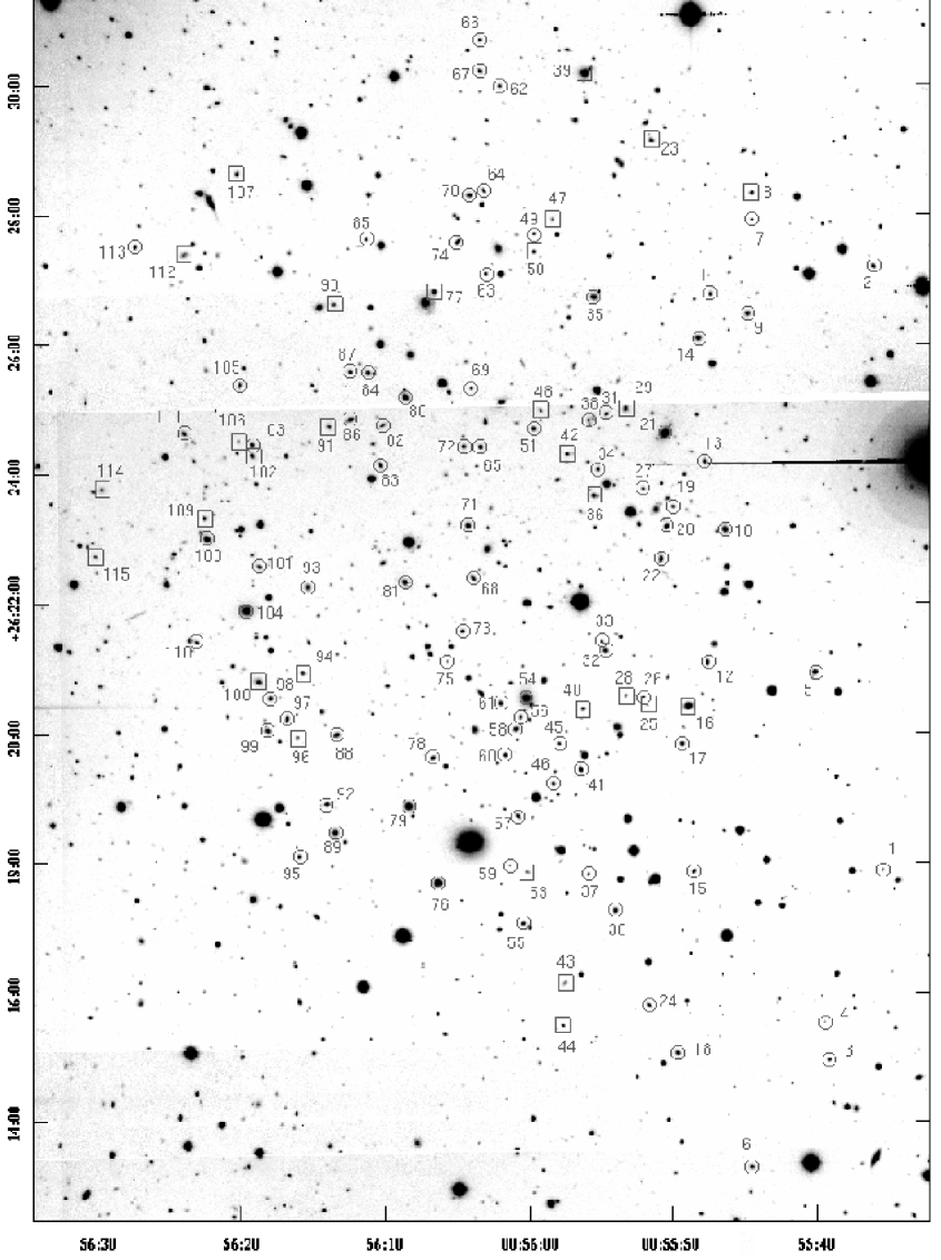
Figure 1: $R$–band image of A115 taken with the WFC camera of the INT. Targets with successful velocity measurements are labeled as in Table 1. Circles and boxes indicate cluster members and non member galaxies, respectively.

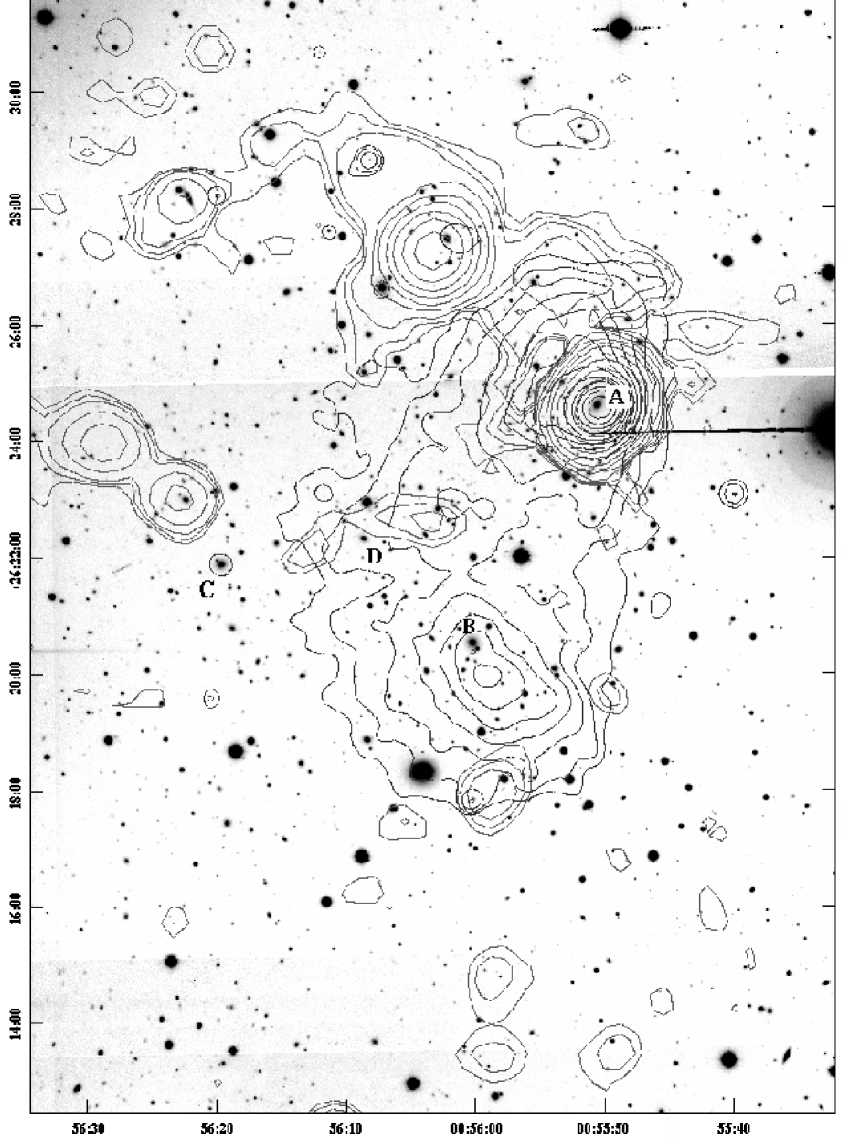
Figure 2: $R$–band image of the cluster A115 with, superimposed, the smoothed contour levels of the Chandra X–ray image ID#3233 (photons in the energy range 0.5–5 keV; blue) and the contour levels of the NVSS (Condon et al. con98 (1998)) radio image (red). Letters A, B, C and D indicate the three brightest cluster members each one corresponding to Beers et al. (bee83 (1983)) clumps and a fourth bright galaxy (see text).

Table 1 lists the velocity catalogue (see also Fig. 1 and Fig. 2): identification number of each galaxy, ID (Col. 1); ID code following the IAU nomenclature (Col. 2); right ascension and declination, $\alpha$ and $\delta$ (J2000, Col. 3); $B$ and $R$ magnitudes (Cols. 4 and 5, respectively); heliocentric radial velocities, ${\rm v}=cz_{\sun}$ with errors, $\Delta{\rm v}$ (Cols. 6 and 7, respectively); spectral classification SC (Col. 8).

3 Analysis & Results

3.1 Member selection and global properties

To select cluster members out of the 115 galaxies having redshifts, we follow the two steps procedure. First, we perform the adaptive–kernel method (hereafter DEDICA, Pisani pis93 (1993) and pis96 (1996); see also Fadda et al. fad96 (1996); Girardi et al. gir96 (1996); Girardi & Mezzetti gir01 (2001)). We find the significant peaks in the velocity distribution $>$99% c.l.. This procedure detects A115 as a one–peak structure at $z\sim 0.1937$ populated by 88 galaxies considered as candidate cluster members (see Fig. 3). Out of non–member galaxies, 12 and 15 are foreground and background galaxies, respectively.

Figure 3: Redshift galaxy distribution. The solid line histogram refers to galaxies assigned to the cluster according to the DEDICA reconstruction method.

The projected clustercentric distance vs. the rest-frame velocity of the 88 galaxies is shown in Fig. 4 where we also show the three brightest galaxies in our sample, each of them corresponding to a different galaxy density clumps as found by Beers et al. (bee83 (1983)), i.e. IDs 54, 21(=3C28) and 104 (hereafter BCM–B, BCM–A, and BCM–C) corresponding to B (A115S), A (A115N), and C clumps, respectively. The position of BCM–B is very close to that of the southern X–ray peak [R.A.=$00^{\mathrm{h}}55^{\mathrm{m}}58\,\hbox to0.0pt{\hbox{$\mathrm{{}^{s}}$}\hss}{\hbox{$.$}}\,81$, Dec.=$+26\mathrm{{}^{\circ}}\,19\mathrm{{}^{\prime}}\;\,58\,\hbox to0.0pt{\hbox{$\mathrm{{}^{\prime}\hskip-1.00006pt{}^{\prime}}$}\hss}{\hbox{$.$}}\,9$ (J2000.0) as recovered from X–ray Chandra data, see Fig. 2]. BCM–A=3C28 is coincident with the northern X–ray peak and is very close to the position of the X–ray centroid when masking the X–ray emission of the point source [R.A.=$00^{\mathrm{h}}55^{\mathrm{m}}53\,\hbox to0.0pt{\hbox{$\mathrm{{}^{s}}$}\hss}{\hbox{$.$}}\,2$, Dec.=$+26\mathrm{{}^{\circ}}\,24\mathrm{{}^{\prime}}\;\,59\mathrm{{}^{\prime}}\hskip-1.00006pt\mathrm{{}^{\prime}}\;$ (J2000.0) by Govoni et al. 2001b ]. We also consider the bright galaxy ID 81 (hereafter BCM–D, see Sect. 3.3) located in the middle of the above three galaxies.

Figure 4: Projected clustercentric distance vs. rest–frame velocity v_rf=(v-$<$v$>$)$/(1+z)$ for the 88 galaxies in the main peak (see Fig. 3) showing galaxies detected as interlopers by our “shifting gapper” procedure (stars and crosses) when using BCM–A and –B as alternative cluster centres (top and bottom panels, respectively). We reject the three galaxies with highest velocities (stars) to build our basic sample of 85 galaxies and all galaxies indicated by crosses and stars in the top panel to build our Sample2. The three brightest cluster members each one corresponding to Beers et al. (bee83 (1983)) clumps (BCM–A, –B and –C) and a fourth bright galaxy (BCM–D) are indicated by squares.

All the galaxies assigned to the A115 peak are analysed in a second step by applying the “shifting gapper” technique by Fadda et al. (fad96 (1996)), which uses the combination of position and velocity information. This procedure rejects galaxies that are too far in velocity from the main body of galaxies and within a fixed bin that shifts along the distance from the cluster centre. The procedure is iterated until the number of cluster members converges to a stable value. Following Fadda et al. (fad96 (1996)) we use a gap of $1000$ km s${}^{-1}\;$– in the cluster rest–frame – and a bin of 0.6 $h_{70}^{-1}$ Mpc, or large enough to include 15 galaxies. In the case of the A115 complex, which is not an individual system, we fix alternatively BCM–A and –B as cluster centres. Fig. 4 shows the results. The very high velocity galaxy (ID 91) is a clear interloper far more than 3000 km s${}^{-1}\;$from other galaxies. The other two high velocity galaxies (IDs 96 and 100), that are close enough in 2D and far from the high velocity BCM–A galaxy (see Fig. 1), are rejected in both our analyses. The conclusion about the low velocity tail is less clear also because few of these galaxies lie in the eastern region of the cluster and might be associated to the C clump (or to the D clump, see Sect. 3.3). We decide to define 85 likely cluster members rejecting the three highest velocity galaxies (basic sample). In some analyses we also consider an alternative sample of 80 galaxies – Sample2 – also rejecting the low velocity galaxies indicated in Fig. 4 (the crosses in the middle panel).

By applying the bi-weight estimator to cluster members (Beers et al. bee90 (1990)), we compute a mean cluster redshift of $\left<z\right>=0.1929\pm$ 0.0005, i.e. $\left<\rm{v}\right>=57817\pm$148 km s^-1. We estimate the LOS velocity dispersion, $\sigma_{\rm v}$, by using the bi-weight estimator and applying the cosmological correction and the standard correction for velocity errors (Danese et al. dan80 (1980)). We obtain $\sigma_{\rm v}=1362_{-108}^{+126}$ km s^-1, where errors are estimated through a bootstrap technique. Consistent results are found for Sample2 (see Table 2).

Table 2: Results of the kinematical analysis.

$$\begin{array}[]{l r l l c}\hline\cr\vskip 3.0pt plus 1.0pt minus 1.0pt\cr\hline\cr\vskip 3.0pt plus 1.0pt minus 1.0pt\cr\mathrm{Sample}&\mathrm{N_{g}}&\phantom{249}\mathrm{<v>}\phantom{249}&\phantom{24}\sigma_{\rm v}^{\mathrm{a}}\phantom{24}&\mathrm{BCM\ galaxies}\\ &&\phantom{249}\mathrm{km\ s^{-1}}\phantom{249}&\phantom{2}\mathrm{km\ s^{-1}}\phantom{24}&\\ \hline\cr\vskip 3.0pt plus 1.0pt minus 1.0pt\cr\mathrm{Whole\ system}&85&57817\pm 148&1362_{-108}^{+126}&\mathrm{A,B,C,D}\\ \mathrm{Whole\ system\ Sample2}&80&57956\pm 132&1175_{-76}^{+95}&\mathrm{A,B,C}\\ \mathrm{WGAP1}&8&54448\pm 212&529_{-44}^{+124}&\mathrm{D}\\ \mathrm{WGAP2}&6&55912\pm 78&162_{-55}^{+39}&\\ \mathrm{DS-A}&11&59199\pm 263&816_{-103}^{+128}&\mathrm{A}\\ \mathrm{DS-C}&3&56138\pm 1001&-&\mathrm{C}\\ \mathrm{KMM1}&10&54819\pm 299&873_{-114}^{+225}&\mathrm{D}\\ \mathrm{KMM2}&44&57833\pm 155&1017_{-77}^{+109}&\mathrm{B,C}\\ \mathrm{KMM3}&31&58500\pm 203&1109_{-112}^{+199}&\mathrm{A}\\ \mathrm{CORE-A}&6&59457\pm 364&750_{-153}^{+337}&\mathrm{A}\\ \mathrm{CORE-B}&6&57493\pm 434&894_{-597}^{+290}&\mathrm{B}\\ \mathrm{Passive\ gals}&34&57325\pm 252&1447_{-152}^{+247}&{}^{\mathrm{b}}\mathrm{C,D}\\ \mathrm{Active\ gals}&14&58950\pm 411&1462_{-440}^{+704}&\mathrm{A}\\ \mathrm{Balmer\ abs.\ gals}&9&58988\pm 668&1817_{-994}^{+834}&\\ \mathrm{Emission\ lines\ gals}&5&58558\pm 527&898_{-218}^{+363}&\mathrm{A}\\ \vskip 3.0pt plus 1.0pt minus 1.0pt\cr\hline\cr\vskip 3.0pt plus 1.0pt minus 1.0pt\cr\hline\cr\end{array}$$

• We use the biweigth and the gapper estimators by Beers et al. (1990) for samples with $\mathrm{N_{g}}\geq$ 15 and with $\mathrm{N_{g}}<15$ galaxies, respectively (see also Girardi et al. gir93 (1993)).

• Notice that BCM-B resembles characteristics of a passive galaxy, but it does not appears in our classification since its spectra has $\cal R$ slightly below the threshold value of 7.

Hereafter, for practical reasons, we consider as centre of the whole A115 complex the position of the bi-weight centre obtained using bi-weight mean estimators for R.A. and Dec. separately [R.A.=$00^{\mathrm{h}}56^{\mathrm{m}}01\,\hbox to0.0pt{\hbox{$\mathrm{{}^{s}}$}\hss}{\hbox{$.$}}\,31$, Dec.=$+26\mathrm{{}^{\circ}}22\mathrm{{}^{\prime}}26\,\hbox to0.0pt{\hbox{$\mathrm{{}^{\prime}\hskip-1.00006pt{}^{\prime}}$}\hss}{\hbox{$.$}}\,6$ (J2000.0)].

3.2 Velocity structure

We analyse the velocity distribution to look for possible deviations from Gaussianity that could provide important signatures of complex dynamics. For the following tests the null hypothesis is that the velocity distribution is a single Gaussian.

We estimate three shape estimators, i.e. the kurtosis, the skewness, and the scaled tail index (see, e.g., Beers et al. bee91 (1991)). The value of the skewness (-0.462) shows evidence that the velocity distribution differs from a Gaussian at the $95-99$% c.l. (see Table 2 of Bird & Beers bir93 (1993)). Moreover, the W–test (Shapiro & Wilk sha65 (1965)) marginally rejects the null hypothesis of a Gaussian parent distribution at the 92% c.l..

Then we investigate the presence of gaps in the distribution. A weighted gap in the space of the ordered velocities is defined as the difference between two contiguous velocities, weighted by the location of these velocities with respect to the middle of the data. We obtain values for these gaps relative to their average size, precisely the midmean of the weighted–gap distribution. We look for normalized gaps larger than 2.25 since in random draws of a Gaussian distribution they arise at most in about 3% of the cases, independent of the sample size (Wainer and Schacht wai78 (1978); see also Beers et al. bee91 (1991)). Two significant gaps in the ordered velocity dataset are detected individuating two groups in the low velocity tail of the velocity distribution, of eight and six galaxies (see WGAP1 and WGAP2 in Table 2 and Fig. 5).

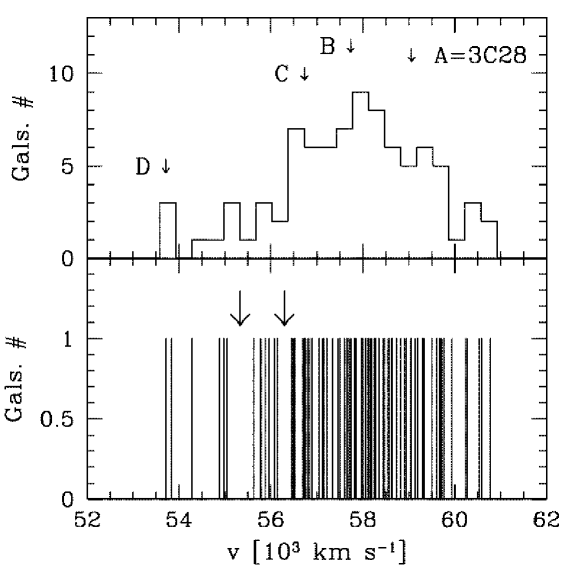
Figure 5: Top panel: velocity distribution of the 85 fiducial cluster members. Arrows correspond to the bright galaxies BCM–A, –B, –C and –D). Bottom panel: stripe density plot where the arrows indicate the positions of the significant gaps. The gap at the lower velocity has a normalized size =2.41, the other =2.25).

We use the results of the gap analysis to determine the first guess when using the Kaye’s mixture model (KMM) to find a possible group partition of the velocity distribution (as implemented by Ashman et al. ash94 (1994)). The KMM algorithm fits an user–specified number of Gaussian distributions to a dataset and assesses the improvement of that fit over a single Gaussian. In addition, it provides the maximum–likelihood estimate of the unknown n–mode Gaussians and an assignment of objects into groups. We do not find any two– or three–groups partition which is a significant better descriptor of the velocity distribution with respect to a single Gaussian.

3.3 2D galaxy distribution

When applying the DEDICA method to the 2D distribution of A115 galaxy members we find three significant peaks. The position of the highest peak is close to the location of the BCM–B and of the southern peak of X–ray emission (XS in Fig.6). Another peak is close to the location of the BCM–A, of the northern peak of X–ray emission (XN) and of the X–ray centroid when masking the X–ray emission of the point source (X, Govoni et al. 2001b ). When dividing the sample in bright and faint galaxies – using the median magnitude value $R$=18.32 – we find that the 2D distributions of the two samples are different at the 98.5% c.l. according to the two–dimensional Kolmogorov–Smirnov test (hereafter 2DKS–test; see Fasano & Franceschini fas87 (1987), as implemented by Press et al. pre92 (1992)). In fact, the faint galaxies sample shows both peaks A and B, while the bright galaxies sample only shows the peak B.

Figure 6: Spatial distribution on the sky of spectroscopically confirmed cluster members and the relative isodensity contour map. The three brightest galaxies BCM–A –B, and –C corresponding to Beers et al. (bee83 (1983)) groups, a fourth bright galaxy (BCM–D) and the X–ray peaks are indicated by large squares, too. The plot is centred on the cluster centre defined as the bi-weight centre (see text).

Our spectroscopic data do not cover the entire cluster field and suffer from magnitude incompleteness. To overcome these limits we recover our photometric catalogue selecting likely members on the basis of the colour–magnitude relation (hereafter CMR), which indicates the early–type galaxy locus. To determine CMR we fix the slope according to López–Cruz et al. (lop04 (2004), see their Fig. 3) and apply the two–sigma–clipping fitting procedure to the cluster members obtaining $B$–$R=3.611-0.069\times R$ (see Fig. 7). Out of our photometric catalogue we consider galaxies (objects with SExtractor stellar index $\leq 0.9$) lying within 0.25 mag of the CMR. To avoid contamination by field galaxies we do not show results for galaxies fainter than 21 mag (in $R$–band). The contour map for 369 likely cluster members having $R\leq 21$ shows again the two peaks in correspondence of BCM–A and BCM–B and also a peak in correspondence of BCM–C. Finally, a less dense peak lies in the middle of the above three peaks and corresponds to the luminous galaxy BCM–D at a very low velocity (see Fig. 8). Similar results are found analysing the 268 galaxies with $R\leq 20$. The analysis of 136 galaxies with $R\leq 19$ shows as very significant only the southern peak close to BCM–B in agreement with the results coming from the spectroscopic sample (see above).

Figure 7: $B$–$R$ vs. $R$ diagram for galaxies with available spectroscopy is shown by small dots and crosses (cluster and field members, respectively). Large solid dots indicate luminous galaxies BCM–A, –B, –C and –D. The solid line gives the best–fit colour–magnitude relation as determined on member galaxies; the dashed lines are drawn at $\pm$0.25 mag from the CMR. Large open symbols indicates classified galaxies: circles (“k”), squares (“k+a”), rombs (“a+k”), triangles (“e(c)”), and stars (“e(a)”/“e(b)”).

Figure 8: Spatial distribution on the sky and relative isodensity contour map of 369 likely cluster members (according to the colour–magnitude relation) with $R\leq 21$, obtained with the DEDICA method. The three brightest galaxies BCM–A –B, and –C are indicated by large circles and the X–ray peaks are indicated by large squares. It is also shown the position of the luminous galaxy BCM–D. The plot is centred on the cluster centre.

3.4 Position–velocity correlations

The existence of correlations between positions and velocities of cluster galaxies is a footprint of real substructures. Here we use different approaches to analyse the structure of A115 combining velocity and position information.

The cluster velocity field may be influenced by the presence of internal substructures. To investigate the velocity field of the A115 complex we divide galaxies in a low and a high velocity samples by using the median cluster velocity and check the difference between the two distributions of galaxy positions. Fig. 9 shows that low and high velocity galaxies are segregated roughly in the E–W direction. The two distributions are different at the 99.5% c.l. according to the 2DKS–test. In order to estimate the direction of the velocity gradient we perform a multiple linear regression fit to the observed velocities with respect to the galaxy positions in the plane of the sky (see also den Hartog & Katgert den96 (1996); Girardi et al. gir96 (1996)). We find a position angle on the celestial sphere of $PA=269_{-18}^{+19}$ degrees (measured counter–clock–wise from north), i.e. higher velocity galaxies lie in the western region of the cluster (see Fig. 9). To assess the significance of this velocity gradient we perform 1000 Monte Carlo simulations by randomly shuffling the galaxy velocities and for each simulation we determine the coefficient of multiple determination ($RC^{2}$, see e.g., NAG Fortran Workstation Handbook nag86 (1986)). We define the significance of the velocity gradient as the fraction of times in which the $RC^{2}$ of the simulated data is smaller than the observed $RC^{2}$. We find that the velocity gradient is marginally significant at the 90% c.l.. Similar results are obtained for the Sample2 ($PA=267_{-17}^{+18}$ degrees at the 91% c.l.).

Figure 9: Spatial distribution on the sky of 85 cluster members. Open and solid circles indicate low and high velocity galaxies, the cross the galaxy with median velocity. The larger the symbol, the smaller is the radial velocity. The solid and faint lines indicate the position angle of the cluster gradient and relative errors, respectively. The faint big squares indicate the 14 galaxies belonging to WGAP1 and WGAP2 (see Sect. 3.2). The plot is centred on the cluster centre.

We combine galaxy velocity and position information to compute the $\Delta$–statistics devised by Dressler & Schectman (dre88 (1988)). This test is sensitive to spatially compact subsystems that have either an average velocity that differs from the cluster mean, or a velocity dispersion that differs from the global one, or both. We find $\Delta=121$ for the value of the parameter which gives the cumulative deviation. This value is an indication of substructure, significant at the 96% c.l., as assessed computing 1000 Monte Carlo simulations, randomly shuffling the galaxy velocities. Fig. 10 shows the distribution on the sky of all galaxies, each marked by a circle: the larger the circle, the larger the deviation $\delta_{i}$ of the local parameters from the global cluster parameters, i.e. the higher the evidence for substructure. This figure provides information on the positions of substructures: one in the eastern region corresponding to the clump C and one in the northern region corresponding to the clump A. Similar results obtained for Sample2 ($\Delta=110$ and a c.l. of 95%), but the eastern substructure is no longer so obvious in the relative plot.

Figure 10: Spatial distribution of cluster members, each marked by a circle: the larger the circle, the larger is the deviation $\delta_{i}$ of the local parameters from the global cluster parameters, i.e. there is more evidence for substructure (according to the Dressler & Schectman test, see text). The boldface circles indicate those with $\delta_{i}\geq 2.2$ (see text). The plot is centred on the cluster centre.

To obtain further information, we resort to the technique developed by Biviano et al. (biv02 (2002)), who used the individual $\delta_{i}$–values of the Dressler & Schectman method. The critical point is to determine the value of $\delta_{i}$ that optimally indicates galaxies belonging to substructure. To this aim we consider the $\delta_{i}$–values of all 1000 Monte Carlo simulations already used to determine the significance of the substructure (see above). The resulting distribution of $\delta_{i}$ is compared to the observed one finding a difference of $P>99.99$% c.l. according to the KS–test. The “simulated” distribution is normalized to produce the observed number of galaxies and compared to the observed distribution in Fig. 11: the latter shows a tail at large values. The tail with $\delta\mathrel{\hbox{\hbox to0.0pt{\hbox{\lower 4.0pt\hbox{$\sim$}}\hss}\hbox{$>$}}}2$ is populated by galaxies that presumably are in substructures. For the selection of galaxies within substructures we choose the value of $\delta_{\rm lim}=2.2$, since the galaxies with $\delta_{i}>\delta_{\rm lim}$ are well separated in the sky (see Fig. 10) and assign three and eleven galaxies to the clumps C and A, respectively (hereafter DS–C and DS–A). The northern structure is populated by high velocity galaxies, while the poor statistics prevent us to obtain firm conclusions about the eastern structure (see Table 2).

Figure 11: The distribution of $\delta_{i}$ deviations of the Dressler–Schectman analysis for the 85 member galaxies. The solid line represents the observations, the dashed line the distribution for the galaxies of simulated clusters, normalized to the observed number.

The Gaussian model for the 2D galaxy distribution is poorly supported by theoretical and/or empirical arguments and, however, our galaxy catalogue is not complete down to a magnitude limit. However, since the 3D diagnostics is in general the most sensitive indicators of the presence of substructure (e.g., Pinkney et al. pin96 (1996)), we apply the 3D version of the KMM software using simultaneously galaxy velocity and positions. We use the galaxy assignment given by Dressler–Schectman method to determine the first guess when fitting three groups. The algorithm fits a three–groups partition at the 97% c.l. according to the likelihood ratio test (hereafter KMM1, KMM2, KMM3 groups from low to high mean velocities). The results for the three groups are shown in Table 2 and Fig. 12. KMM1 group is sparse in the sky, but well distinct in velocity from the other two groups. Several of its galaxies were already detected by the weighted gap analysis as belonging to WGAP1 and WGAP2 (see Sect. 3.2). Moreover, KMM1 contains BCM–D. KMM2 and KMM3 groups are well distinct in the sky. KMM2 contains both BCM–B and BCM–C, while KMM3 contains BCM–A.

Figure 12: Spatial distribution on the sky of the 85 member galaxies. Solid circles, open circles and triangles indicate KMM1, KMM2, and KMM3. The large faint squares indicate the position of the brightest cluster members BCM–A, –B, –C and –D. The plot is centred on the cluster centre.

3.5 Kinematics of A115N and A115S

The spatial agreement between the two brightest cluster members (BCM–A and –B) and the peaks of X–ray emission as well as the high density of galaxies around BCM–A and –B prompts us to analyse the profiles of the mean velocity and the velocity dispersion of galaxy systems surrounding these two galaxies (see Figs. 13 and 14, respectively). This allows an independent analysis of the individual galaxy clumps. Although an increase in the velocity–dispersion profile in the cluster central regions might be due to dynamical friction and galaxy merging (e.g., Menci & Fusco–Femiano men96 (1996); Girardi et al. gir98 (1998); Biviano & Katgert biv04 (2004)), in the case of A115 it might be simply induced by the contamination of the galaxies of a secondary clump (e.g., Girardi et al. gir96 (1996); Girardi et al. gir05 (2005)). The latter hypothesis can be investigated by looking at the behaviour of the mean velocity profile.

Since from the above sections we know the presence of one or likely a few low velocity groups, we analyse the Sample2 to avoid, at least partially, the possible contamination. We also consider the results obtained rejecting all galaxies belonging to low velocity WGAP1 and WGAP2. Figs. 13 and 14 show velocity–dispersion and mean–velocity profiles, as well as regions not likely to be contaminated by other galaxy systems and thus reliable for kinematical analysis. Detailed results of this analysis are included in Table 2 where the “uncontaminated” galaxy systems are named as CORE–A and CORE–B.

Fig. 13 shows how the integral velocity–dispersion slightly increases with the distance from the BCM–A. Simultaneously, the mean velocity shows a continuous decline from high values $\sim 59000$ km s${}^{-1}\;$suggesting a strong contamination of galaxies from structures connected with BCM–B, –C and –D, all having lower mean velocities. In a conservative view we consider the likely uncontaminated region within 0.25 $h_{70}^{-1}$ Mpc, where we find $\sigma_{\rm v}\simeq 750$ km s^-1. Fig. 14 shows an enough robust mean velocity and a sharp increase of the integral velocity–dispersion with the distance from the BCM–B up to a peak value $\sim 1450$ km s${}^{-1}\;$at $\sim 0.3$ $h_{70}^{-1}$ Mpc. We interpret these features as the contamination of the structures connected with BCM–A, –C and –D with higher and lower mean velocities. Their combination does not affect the mean velocity but strongly increases the velocity dispersion. In fact, the peak value of the velocity dispersion goes down from 1450 to 1200 km s${}^{-1}\;$when rejecting low velocity galaxies of WGAP1 and WGAP2. We then consider the likely uncontaminated region within 0.25 $h_{70}^{-1}$ Mpc, where we find $\sigma_{\rm v}\simeq 900$ km s^-1.

Figure 13: Kinematical profiles of the northern subcluster A115N obtained assuming BCM–A as centre. The vertical line indicates the region likely not contaminated from other galaxy clumps (see text). Top panel: rest–frame velocity vs. projected distance from the subcluster centre (BCM–A): crosses indicate the galaxies belonging to WGAP1 and WGAP2. Differential (big circles) and integral (small points) mean velocity and LOS velocity–dispersion profiles are shown in middle and bottom panels, respectively. For the differential profiles we plot the values for seven annuli from the centre of the subcluster, each of 0.25 $h_{70}^{-1}$ Mpc. For the integral profiles, the mean and dispersion at a given (projected) radius from the subcluster–centre is estimated by considering all galaxies within that radius – the first value computed on the five galaxies closest to the centre. The error bands at the $68\%$ c.l. are also shown. In the bottom panel, the horizontal line represents the range of X–ray temperatures as given in the literature for A115N (see Sect. 1) transformed in $\sigma_{\rm v}$ assuming the density–energy equipartition between gas and galaxies, i.e. $\beta_{\rm spec}=1$ (see text).

Figure 14: The same as in Fig. 13, but referring to the southern subcluster A115S centred around BCM–B. The dashed line in the bottom panel gives the integral velocity dispersion profile when rejecting the low velocity galaxies of WGAP1 and WGAP2. In the bottom panel, the horizontal line represents the range of X–ray temperatures as given in the literature for A115S (see Sect. 1) transformed in $\sigma_{\rm v}$ assuming the density–energy equipartition between gas and galaxies, i.e. $\beta_{\rm spec}=1$ (see text).

4 3D structure and virial mass of A115

On the basis of the above section we conclude that A115 is formed by two subclusters well distinct in the sky and centred around BCM–A and –B, hereafter A115N and A115S, with the addition of several low velocity galaxies, above all in the eastern cluster region, likely organised in small groups (see Fig. 9 and the PA of the velocity gradient).

As for the low velocity groups we detect two 2D galaxy concentrations around the two bright, low velocity galaxies BCM–C and –D. Moreover, we find two possible groups in the low velocity tail of the velocity distribution (WGAP1 containing BCM–D and WGAP2). The Dressler–Schectman test detects a substructure around the BCM–C, too. The presence of a group around BCM–D finds some support in the faint X–ray emission shown there (see Gutierrez & Krawczynski gut05 (2005) and Fig. 2). That we find evidence of a few groups rather than of an individual massive cluster agrees with the absence of a third X–ray luminous peak.

As for A115N, we find comparable kinematical properties in the analysis of DS–A and CORE–A, i.e. $\left<\rm{v}\right>\mathrel{\hbox{\hbox to0.0pt{\hbox{\lower 4.0pt\hbox{$\sim$}}\hss}\hbox{$>$}}}$ 59000 km s${}^{-1}\;$and $\sigma_{\rm v}\sim$ 800 km s^-1. Instead KMM3 is contaminated by the presence of low velocity galaxies, e.g. IDs 10 and 19 close to BCM–A. As for A115S, we find $\left<\rm{v}\right>\sim$ 57500 km s${}^{-1}\;$and $\sigma_{\rm v}\sim$ 900–1000 km s${}^{-1}\;$(see KMM2 and CORE–B). The velocity dispersion of the two subclusters are roughly comparable to their average X–ray temperature as listed in the literature and transformed in $\sigma_{\rm v}$ assuming the density–energy equipartition between gas and galaxies, i.e. $\beta_{\rm spec}=1$ (see Figs. 13 and 14). The two subclusters differ by $\sim 2000$ km s${}^{-1}\;$in the LOS velocity, i.e. almost three times more than what found by Beers et al. (bee83 (1983)) with only 19 cluster members. In agreement with Beers et al. (bee83 (1983)), we find that A115S is dynamically somewhat more important than A115N, while the contrary is found by X–ray data (Jones & Forman jon99 (1999); White et al. whi97 (1997); Gutierrez & Krawczynski gut05 (2005); but see Shibata et al. shi99 (1999)). As already suggested by Beers et al. (bee83 (1983)) the presence of 3C28 might affects the X–ray results overestimating the X–ray luminosity and the temperature of A115N.

Although A115 is likely in a phase of interaction (see the following section), the two main galaxy subclusters are still well detectable and roughly well coincident with the X–ray peaks. Thus we assume that each subcluster is in dynamical equilibrium to compute virial quantities. Hereafter we assume $\sigma_{\rm v}=$ 750–850 km s${}^{-1}\;$and 900–1000 km s${}^{-1}\;$for A115N and A115S, respectively.

Following the prescriptions of Girardi & Mezzetti (gir01 (2001)), we assume for the radius of the quasi–virialized region R${}_{\rm vir,N}=0.17\times\sigma_{\rm v}/H(z)=2.2$–2.5 $h_{70}^{-1}$ Mpc and R${}_{\rm vir,S}=2.6$–2.9 $h_{70}^{-1}$ Mpc for A115N and A115S, respectively – see their eq. 1 after introducing the scaling with $H(z)$ (see also eq.  8 of Carlberg et al. car97 (1997) for R₂₀₀). Therefore, our spectroscopic catalogue samples most of the virialized region.

One can compute the mass using the virial theorem (Limber & Mathews lim60 (1960); see also, e.g., Girardi et al. gir98 (1998)) under the assumption that mass follows galaxy distribution: $M=M_{\rm svir}-\rm{SPT}$, where $M_{\rm svir}=3\pi/2\cdot\sigma_{\rm v}^{2}{\rm R}_{\rm PV}/G$ is the standard virial mass, R_PV a projected radius (equal two times the harmonic radius), and SPT is the surface pressure term correction (The & White the86 (1986)). The value of R_PV depends on the size of the considered region, so that the computed mass increases (but not linearly) with the increasing considered region. Since the two subclusters are interacting and we do not cover the whole virialized region we use an alternative estimate which was shown be good when R_PV is computed within R_vir (see eq. 13 of Girardi et al. gir98 (1998)). This alternative estimate is based on the knowledge of the galaxy distribution and, in particular, a galaxy King–like distribution with parameters typical of nearby/medium–redshift clusters: a core radius R${}_{\rm core}=1/20\times{\rm R}_{\rm vir}$ and a slope–parameter $\beta_{\rm fit}=0.8$, i.e. the volume galaxy density at large radii as $r^{-3\beta_{\rm fit}}=r^{-2.4}$ (Girardi & Mezzetti gir01 (2001)). For the whole virialized region we obtain R${}_{\rm PV,N}=1.6$–1.8 $h_{70}^{-1}$ Mpc and R${}_{\rm PV,S}=$1.9–2.2 $h_{70}^{-1}$ Mpc. As for the SPT correction, we assume a 20% computed combining data on many clusters one (e.g., Carlberg et al. car97 (1997); Girardi et al. gir98 (1998)). This leads to virial masses $M_{\rm N}(<{\rm R}_{\rm vir,N}=2.2-2.5\,\;h_{70}^{-1}\mathrm{Mpc})=8.0$–11.6 $\times 10^{14}\;h_{70}^{-1}\;M_{\odot}\;$and $M_{\rm S}(<{\rm R}_{\rm vir,S}=2.6-2.9\,\;h_{70}^{-1}\mathrm{Mpc})=13.8$ –18.9 $\times 10^{14}\;h_{70}^{-1}\;M_{\odot}\;$for the two subclusters.

To compare our results with the estimate recovered from a X–ray surface brightness deprojection analysis (White et al. whi97 (1997)) we assume that each subcluster is described by a King–like mass distribution (see above) or, alternatively, a NFW profile where the mass–dependent concentration parameter is taken from Navarro et al. (nav97 (1997)) and rescaled by the factor $1+z$ (Bullock et al. bul01 (2001); Dolag et al. dol04 (2004)). We obtain $M_{\rm N}(<{\rm R}_{\rm out,N}=0.235\,\;h_{70}^{-1}\mathrm{Mpc})=(4.2-9.9)$ $\times 10^{13}\;h_{70}^{-1}\;M_{\odot\;}$and $M_{\rm S}(<{\rm R}_{\rm out,S}=0.157\,\;h_{70}^{-1}\mathrm{Mpc})=(2.5-5.5)$ $\times 10^{13}\;h_{70}^{-1}\;M_{\odot}$. The first estimate is somewhat smaller and the second one is in agreement with those found by White et al. (whi97 (1997), see their Table 3 where $M_{\rm grav,N}(<{\rm R}_{\rm out,N})=14.0$ $\times 10^{13}\;h_{70}^{-1}\;M_{\odot\;}$and $M_{\rm grav,S}(<{\rm R}_{\rm out,S})=5.0$ $\times 10^{13}\;h_{70}^{-1}\;M_{\odot\;}$in our cosmology).

As for the mass of the whole system, the contribution of the low velocity groups is of minor importance since they likely have low velocity dispersion and the virial mass scales with $\sigma_{\rm v}^{3}$. E.g., we estimate that $M\sim 2.4$ $\times 10^{14}\;h_{70}^{-1}\;M_{\odot}\;$for a $\sigma_{\rm v}\sim 500$ km s${}^{-1}\;$group (see WGAP1 in Table 2). Considering the possible presence of, at most, two of these $\sigma_{\rm v}\sim 500$ km s${}^{-1}\;$groups, a reliable mass estimate of the whole system is then M=2.2–3.5 $\times 10^{15}\;h_{70}^{-1}\;M_{\odot}$, in agreement with rich clusters reported in the literature (e.g., Girardi et al. gir98 (1998); Girardi & Mezzetti gir01 (2001)). A smaller mass estimate is given by Govoni et al. [2001b ; $M(<\rm{R=2.3}\,\;h_{70}^{-1}\mathrm{Mpc})=0.6$–1.2 $\times 10^{15}\;h_{70}^{-1}\;M_{\odot}\;$centred on the X–ray centroid in A115N], but notice that it refers to a smaller cluster region, i.e. likely excluding a large part of A115S.

5 Merging scenario

Since A115N and A115S are well detectable and optical and X–ray data indicate a very similar location we are likely looking at the cluster prior to merging. However, A115N and A115S subclusters are already starting to interact, as suggested by several pieces of evidence: the slight displacement between peaks of gas distribution and of galaxy distribution (see our Fig. 8); the presence of an hot region likely due to the interaction (Shibata et al. shi99 (1999); Gutierrez & Krawczynski gut05 (2005)). Very noticeably, the largest dimension of the radio relic is somewhat perpendicular to the axis connecting A115N and A115S in agreement with being originated by shock waves connected to the ongoing merger (e.g., Ensslin & Brüggen ens02 (2002)).

When the merging scenario is assumed to explain the presence of the hot region located between A115N and A115S, a relative colliding velocity is necessary to heat up the ICM temperature $kT$ from $\sim 4$ to $\sim 9$ keV (see Gutierrez & Krawczynski gut05 (2005)). Assuming that the two subclusters are to cause a head–on collision and that their kinetic energies are completely converted to thermal energy, the necessary value of the colliding velocity is ${\rm v}_{\rm coll}=(3k\Delta T/\mu m_{\rm p})^{1/2}$ (see Shibata et al. shi99 (1999)). We find ${\rm v}_{\rm coll}\sim 1600$ km s${}^{-1}\;$in good agreement with the observed relative LOS velocity in the rest frame ${\rm V}_{\rm r}=1646$ km s${}^{-1}\;$as recovered from CORE–A and CORE–B in the cluster rest frame, i.e. ($<$v$>_{\rm CORE-A}$-$<$v$>_{\rm CORE-B})/(1+z)$).

5.1 Bimodal model

Here we investigate the relative dynamics of A115N and A115S using different analytic approaches which are based on an energy integral formalism in the framework of locally flat spacetime and Newtonian gravity (e.g., Beers et al. bee82 (1982)). The values of the relevant observable quantities for the two–clumps system are: the relative LOS velocity in the rest frame, ${\rm V}_{\rm r}=1646$ km s${}^{-1}\;$(as recovered from CORE–A and CORE–B); the projected linear distance between the two clumps, $D=0.89$ $h_{70}^{-1}$ Mpc (as recovered from BCM–A and –B cluster rest frame); the mass of the system obtained by adding the masses of the two subclusters each within its virial radius, log$M_{\rm sys}=15.4107_{-0.0734}^{+0.0734}$ (see Sect. 4).

First, we consider the Newtonian criterion for gravitational binding stated in terms of the observables as ${\rm V}_{\rm r}^{2}D\leq 2GM_{\rm sys}\sin^{2}\alpha\cos\alpha$, where $\alpha$ is the projection angle between the plane of the sky and the line connecting the centres of two clumps. The faint curve in Fig. 15 separates the bound and unbound regions according to the Newtonian criterion (above and below the curve, respectively). Considering the value of $M_{\rm sys}$, the A115N+S system is bound between $20\mathrm{{}^{\circ}}$ and $84\mathrm{{}^{\circ}}$; the corresponding probability, computed considering the solid angles (i.e., $\int^{84^{\rm o}}_{20^{\rm o}}\cos\,\alpha\,d\alpha$), is 65%. We also consider the implemented criterion ${\rm V}_{\rm r}^{2}D\leq 2GM\sin^{2}\alpha_{\rm v}\cos\alpha_{\rm d}$, which introduces different angles $\alpha_{\rm d}$ and $\alpha_{\rm v}$ for projection of distance and velocity, not assuming strictly radial motion between the clumps (Hughes et al. hug95 (1995)). We obtain a binding probability of 60%.

Then, we apply the analytical two–body model introduced by Beers et al. (bee82 (1982)) and Thompson (tho82 (1982); see also Lubin et al. lub98 (1998) for a recent application). This model assumes radial orbits for the clumps with no shear or net rotation of the system. Furthermore, the clumps are assumed to start their evolution at time $t_{0}=0$ with separation $d_{0}=0$, and are moving apart or coming together for the first time in their history; i.e. we are assuming that we are seeing the cluster prior to merging (at the time t=11.106 Gyr at the cluster redshift). The bimodal model solution gives the total system mass $M_{\rm sys}$ as a function of $\alpha$ (e.g., Gregory & Thompson gre84 (1984)). Fig. 15 compares the bimodal–model solutions with the observed mass of the system, which is the most uncertain observational parameter. The present bound outgoing solutions (i.e. expanding), BO, are clearly inconsistent with the observed mass. The possible solutions span these cases: the bound and present incoming solution (i.e. collapsing), BIa and BIb, and the unbound–outgoing solution, UO. For the incoming case there are two solutions because of the ambiguity in the projection angle $\alpha$. We compute the probabilities associated to each solution assuming that the region of $M_{\rm sys}$ values between uncertainties are equally probable for individual solutions: $P_{\rm BIa}\sim 83.5\%$, $P_{\rm BIb}\sim 16.5\%$, $P_{\rm UO}\sim 6\times 10^{-4}$%.

Between the two possible bound solutions, $\alpha\sim$ 21 and 76 degrees, the second one is rather unlikely since it means a distance of $\sim 3.7$ $h_{70}^{-1}$ Mpc between A115N and A115S, i.e. well larger than the virial radii, while the second solution means a distance of $\sim 1.0$ $h_{70}^{-1}$ Mpc in agreement with a certain degree of interaction. When assuming $\alpha=21$ degrees the present colliding velocity is very large ($\sim 4400$ km s^-1) and the cluster cores will cross after 0.08 Gyr.

Figure 15: System mass vs. projection angle for bound and unbound solutions of the two–body model applied to A115N and A115S subclusters (solid and dotted curves, respectively, see text). The thin curve separates the bound and unbound regions according to the Newtonian criterion (above and below the curve, respectively). The horizontal lines give the observational values of the mass system and its uncertainties.

The characterization of the dynamics of A115 using these models is affected by several limitations. For instance, possible underestimates of the masses – e.g., if the subclusters extend outside the virial radius – lead to binding probabilities larger than those computed above. The models do not take the mass distribution in the subclusters into account when the separation of the subclusters is comparable with their size (i.e. at small $\alpha$) and do not consider the possible effect of small, low velocity groups. Moreover, the two–body model breaks down in a regime where A115N and A115S subclusters are already strongly interacting.

Finally, the two–body model does not consider the possibility of an off–axis merger as suggested by the X–ray surface brightness distribution (Gutierrez & Krawczynski gut05 (2005)). For an analytical treatment which assumes that A115N and A115S are in a circular Keplerian orbit with the orbital plane perpendicular to the LOS, we refer to those authors.

As for the low velocity groups, we consider a group corresponding to WGAP1 likely centred around BCM–D and possibly interacting with the A115N+S complex. The values of the relevant observable quantities for the two–clumps system are then: the relative LOS velocity in the rest frame, $V_{\rm r}=3376$ km s${}^{-1}\;$(as recovered from WGAP1 and the mean velocity of CORE–A and CORE–B cluster rest frame); the projected linear distance between the two clumps, $D=0.89$ $h_{70}^{-1}$ Mpc (as recovered from BCM–D and the mean position between BCM–A and –B); the mass of the system obtained by adding the mass of a $\sigma_{\rm v}\sim 500$ km s${}^{-1}\;$group to A115N+S, i.e. log$M_{\rm sys}=15.4427_{-0.0625}^{+0.0625}$. According to the Newtonian criterion for gravitational binding we find a binding probability of 38%. The bimodal model indicates that the group is infalling onto the A115N+S complex with a merging axis intermediate between the LOS and the plane of sky (i.e., $\alpha\sim$40–60 degrees).

5.2 Active galaxies

It has been suggested that cluster–cluster collisions may trigger star formation in cluster galaxies (Bekki bek99 (1999); Moss & Whittle mos00 (2000); Girardi & Biviano gir02 (2002) and references therein). Caldwell & Rose (cal97 (1997)) noticed that post–starburst galaxies are frequently found in clusters with evidence of past collision events. Here we analyse possible segregations between passive and active galaxy populations.

Out of 85 cluster members we classify 48 galaxies finding 34 “passive” galaxies (“k” in Table 1) and 14 “active” galaxies (i.e., 9 “k+a”/“a+k” and 5 “e” galaxies, respectively), see also Fig. 7.

The velocity distribution of passive galaxies differs from that of active galaxies at the 99.47% c.l. according to the KS–test, active galaxies having a larger mean velocity (see Table 2). With present data this difference seems due to both Balmer absorption lines (“k+a”/“a+k”) and emission lines “e” galaxies. This suggests that the galaxy population of the high velocity subcluster (A115N) is very active with respect to other A115 galaxies. Indeed, we find that two out three classified galaxies in CORE–A are active galaxies (in particular BCM–A), while no active galaxy is found in CORE–B. That A115S has a rich, red galaxy population is also found by Rakos et al. (rak00 (2000)) suggesting that this system is evolutionarily “developed”. Analysing the 2D distributions we only find a marginal difference between passive and Balmer absorption lines galaxies (at the 92% c.l. according to the 2dKS–test) with three out of nine Balmer absorption lines galaxies closely located to BCM–A. Assuming that galaxy activity is connected with the merging phenomena, our results point out that A115N subcluster is more affected than A115S in agreement with our finding that A115N is less massive than A115S (see Sect. 4).

6 Summary & conclusions

We present the results of the dynamical analysis of the rich, X–ray luminous, and hot cluster of galaxies A115, showing a binary apparency (A115N and A115S) and containing a diffuse arc–shape radio emission, connected to A115N. This emission is considered a very anomalous relic since elongated relics are generally located at the cluster periphery, and with the largest dimension roughly perpendicular to the cluster radial orientation.

Our analysis is based on new redshift data for 115 galaxies, measured from spectra obtained at the TNG in a cluster region within a radius of 15^′$\times$ 20$\mathrm{{}^{\prime}}\;$. We also use new photometric data obtained at the INT telescope in a field larger than 30^′$\times$30$\mathrm{{}^{\prime}}\;$.

We select 85 cluster members around $z\sim 0.193$ and compute a global LOS velocity dispersion of galaxies, $\sigma_{\rm v}=1362_{-108}^{+126}$ km s^-1.

Our analysis confirms the presence of two structures of cluster–type well recognizable in the plane of the sky and shows that they differ by $\sim 2000$ km s${}^{-1}\;$in LOS velocity. The northern, high velocity subcluster (A115N) is likely centred on the second brightest cluster galaxy (BCM–A, coincident with radio source 3C28) and the northern X–ray peak. The southern, low velocity subcluster (A115S) is likely centred on the first brightest cluster galaxy (BCM–B) and the southern X–ray peak. We estimate that A115S is slightly dynamically more important than A115N having a velocity dispersion of $\sigma_{\rm v}=900-1100$ km s${}^{-1}\;$vs. $\sigma_{\rm v}=750-850$ km s^-1. The virial mass estimates for the two subclusters are $M_{\rm N}(<{\rm R}_{\rm vir,N}=2.2-2.5\,\;h_{70}^{-1}\mathrm{Mpc})=8.0$–11.6 $\times 10^{14}\;h_{70}^{-1}\;M_{\odot}$ and $M_{\rm S}(<{\rm R}_{\rm vir,S}=2.6-2.9\,\;h_{70}^{-1}\mathrm{Mpc})=13.8$ –18.9 $\times 10^{14}\;h_{70}^{-1}\;M_{\odot}$.

Moreover, we find evidence for two small groups at low velocities. In fact, the galaxy distribution obtained from our INT data shows the presence of two concentrations (C and D) in addition to A115N and A115S (A and B). The C group surrounds the third brightest cluster member and coincides with the clump already found by Beers et al. (bee83 (1983); see also our Dressler–Schectman analysis). The D group surrounds another bright galaxy (BCM–D in this paper) and likely coincides with a faint X–ray emission shown by Chandra data (Gutierrez & Krawczynski gut05 (2005)).

Considering the complex structure of A115 we estimate a global cluster virial mass of 2.2–3.5 $\times 10^{15}\;h_{70}^{-1}\;M_{\odot}$.

Our results agree with a pre–merging scenario where A115N and A115S are colliding with a LOS impact velocity $\Delta{{\rm v}_{\rm rf}}\sim 1600$ km s${}^{-1}\;$. The most likely solution to the two–body problem suggests that the merging axis lies at $\sim 20$ degrees from the plane of the sky and that the cores will cross after $\sim 0.1$ Gyr.

In our scenario where 1) A115S is more massive than A115N; 2) the dynamically important axis is the axis connecting the two merging subclusters; 3) this axis is perpendicular to the largest dimension of the relic, the anomaly of the A115 radio diffuse source is likely overcome supporting its relic nature (Govoni et al. 2001b ).

Table 1: This data will be availabe just after publication in A&A.

$$\begin{array}[]{r c c c c c r c}\hline\cr\vskip 3.0pt plus 1.0pt minus 1.0pt\cr\hline\cr\vskip 3.0pt plus 1.0pt minus 1.0pt\cr\mathrm{ID}&\mathrm{IAU\,\,ID}&\mathrm{\alpha},\mathrm{\delta}\,(\mathrm{J}2000)&\mathrm{B}&\mathrm{R}&\mathrm{v}&\mathrm{\Delta}\mathrm{v}&\mathrm{SC}\\ &&00^{\mathrm{h}},+26^{\mathrm{o}}&&&\,\,\,\,\,\,\,\mathrm{(\,km}&\mathrm{s^{-1}\,)}&\\ \hline\cr\vskip 3.0pt plus 1.0pt minus 1.0pt\cr\vskip 3.0pt plus 1.0pt minus 1.0pt\cr\hline\cr\vskip 3.0pt plus 1.0pt minus 1.0pt\cr\hline\cr\end{array}$$

Table 1: Continued.

$$\begin{array}[]{r c c c c c r c}\hline\cr\vskip 3.0pt plus 1.0pt minus 1.0pt\cr\hline\cr\vskip 3.0pt plus 1.0pt minus 1.0pt\cr\mathrm{ID}&\mathrm{IAU\,\,ID}&\mathrm{\alpha},\mathrm{\delta}\,(\mathrm{J}2000)&\mathrm{B}&\mathrm{R}&\mathrm{v}&\mathrm{\Delta}\mathrm{v}&\mathrm{SC}\\ &&00^{\mathrm{h}},+26^{\mathrm{o}}&&&\,\,\,\,\,\,\,\mathrm{(\,km}&\mathrm{s^{-1}\,)}&\\ \hline\cr\vskip 3.0pt plus 1.0pt minus 1.0pt\cr\vskip 3.0pt plus 1.0pt minus 1.0pt\cr\hline\cr\vskip 3.0pt plus 1.0pt minus 1.0pt\cr\hline\cr\end{array}\\$$

References

- (1) Abell, G. O., Corwin, H. G. Jr., & Olowin, R. P. 1989, ApJS, 70, 1
- (2) Ashman, K. M., Bird, C. M. & Zepf, S. E. 1994, AJ, 108, 2348
- (3) Bardelli, S., Zucca, E., Vettolani, G., et al. 1994, MNRAS, 267, 665
- (4) Barrena, R., Biviano, A., Ramella, M., Falco, E. E., & Seitz, S. 2002, A&A, 386, 816
- (5) Barrena, R., Boschin, W., Girardi, M., & Spolaor, M. 2007, A&A, in press (astro-ph/0701833)
- (6) Beers, T. C., Flynn, K. & Gebhardt, K. 1990, AJ, 100, 32
- (7) Beers, T. C., Forman, W., Huchra, J. P., Jones, C., & Gebhardt, K. 1991, AJ, 102, 1581
- (8) Beers, T. C., Geller, M. J., & Huchra, J. P. 1982, ApJ, 257, 23
- (9) Beers, T. C., Geller, M. J., & Huchra, J. P. 1983, ApJ, 264, 365
- (10) Bekki, K. 1999, ApJ, 510, L15
- (11) Bertin, E. & Arnouts, S. 1996, A&AS, 117, 393
- (12) Bird, C. M., & Beers, T. C. 1993, AJ, 105, 1596
- (13) Biviano, A., & Katgert 2004, A&A, 424, 779
- (14) Biviano, A., Katgert, P., Thomas, T., & Adami, C. 2002, A&A, 387, 8
- (15) Böhringer, H., & Schuecker, P. 2002, in “Merging Processes in Galaxy Clusters”, eds. L. Feretti, I. M. Gioia, & G. Giovannini, Kluwer Ac. Pub., The Netherlands: Observational signatures and statistics of galaxy cluster mergers
- (16) Boschin, W., Girardi, M., Barrena, R., et al. 2004, A&A, 416, 839
- (17) Boschin, W., Girardi, M., Spolaor, M., & Barrena, R. 2006, A&A, 449, 461
- (18) Bullock, J. S., Kolatt, T. S., Sigad, Y., et al. 2001, MNRAS, 321, 559
- (19) Buote, D. A. 2002, in “Merging Processes in Galaxy Clusters”, eds. L. Feretti, I. M. Gioia, & G. Giovannini, Kluwer Ac. Pub., The Netherlands: Optical Analysis of Cluster Mergers
- (20) Burns, J. O., Roettiger, K., Ledlow, M., & Klypin, A. 1994, ApJ, 427, L87
- (21) Burstein, D., & Heiles, C. 1982, AJ, 87, 1165
- (22) Caldwell, N. & Rose, J. A. 1997, AJ, 113, 492
- (23) Carlberg, R. G., Yee, H. K. C., & Ellingson, E. 1997, ApJ, 478, 462
- (24) Condon, J. J., Cotton, W. D., Greisen, E. W., et al. 1998, AJ, 115, 1693
- (25) Cousins, A. W. J., 1976, Mem. R. Astr. Soc, 81, 25
- (26) Crawford, C. S., Allen, S. W., Ebeling, H., Edge, A. C., & Fabian, A. C. 1999, MNRAS, 306, 857
- (27) Danese, L., De Zotti, C., & di Tullio, G. 1980, A&A, 82, 322
- (28) den Hartog, R., & Katgert, P. 1996, MNRAS, 279, 349
- (29) Diaferio, A., Kauffmann, G., Balogh, M. L., et al. 2001, MNRAS, 323, 999
- (30) Dolag, K., Bartelmann, M., Perrotta, F., et al. 2004, A&A, 416, 853
- (31) Dressler, A., & Shectman, S. A. 1988, AJ, 95, 985
- (32) Dressler, A., Smail, I., Poggianti, B. M., et al. 1999, ApJS, 122, 51
- (33) Ellingson, E., & Yee, H. K. C. 1994, ApJS, 92, 33
- (34) Ensslin, T. A., & Brüggen, M. 2002, MNRAS, 331, 1011
- (35) Fadda, D., Girardi, M., Giuricin, G., Mardirossian, F., & Mezzetti, M. 1996, ApJ, 473, 670
- (36) Fasano, G., & Franceschini, A. 1987, MNRAS, 225, 155
- (37) Feretti, L. 1999, MPE Report No. 271
- (38) Feretti, L. 2005, X–Ray and Radio Connections (eds. L. O. Sjouwerman and K. K. Dyer) Published electronically by NRAO, http://www.aoc.nrao.edu/events/xraydio Held 3–6 February 2004 in Santa Fe, New Mexico, USA
- (39) Feretti, L. 2002, The Universe at Low Radio Frequencies, Proceedings of IAU Symposium 199, held 30 Nov – 4 Dec 1999, Pune, India. Edited by A. Pramesh Rao, G. Swarup, and Gopal–Krishna, 2002., p.133
- (40) Feretti, L., Gioia, I. M., Giovannini, G., et al. 1984, A&A, 139, 50
- (41) Forman, W., Bechtold, J., Blair, W., et al. 1981, ApJ,243, 133
- (42) Fujita, Y., Sarazin, C. L., Reiprich, T. H., et al. 2004, ApJ, 616, 157
- (43) Giovannini, G., & Feretti, L. 2002, in “Merging Processes in Galaxy Clusters”, eds. L. Feretti, I. M. Gioia, & G. Giovannini, Kluwer Ac. Pub., The Netherlands: Diffuse Radio Sources and Cluster Mergers
- (44) Giovannini, G., Feretti, L., & Gregorini, L. 1987, A&AS, 69, 171
- (45) Giovannini, G., Feretti, L., Venturi T., Kim, K.–T., & Kronberg, P. P. 1993, ApJ, 406, 399
- (46) Giovannini, G., Tordi, M., & Feretti, L. 1999, New Astronomy, 4, 141
- (47) Girardi, M., & Biviano, A. 2002, in “Merging Processes in Galaxy Clusters”, eds. L. Feretti, I. M. Gioia, & G. Giovannini, Kluwer Ac. Pub., The Netherlands: Optical Analysis of Cluster Mergers
- (48) Girardi, M., Biviano, A., Giuricin, G., Mardirossian, F., & Mezzetti, M. 1993, ApJ, 404, 38
- (49) Girardi, M., Boschin, W., & Barrena, R. 2006, A&A, 455, 45
- (50) Girardi, M., Demarco, R., Rosati, P., & Borgani, S. 2005, A&A, 442, 29
- (51) Girardi, M., Fadda, D., Giuricin, G. et al. 1996, ApJ, 457, 61
- (52) Girardi, M., Giuricin, G., Mardirossian, F., Mezzetti, M., & Boschin, W. 1998, ApJ, 505, 74
- (53) Girardi, M., & Mezzetti, M. 2001, ApJ, 548, 79
- (54) Govoni, F., Ensslin, T. A., Feretti, L., & Giovannini, G. 2001a, A&A, 369, 441
- (55) Govoni, F., Feretti, L., Giovannini, G., et al. 2001b, A&A, 376, 803
- (56) Gregory, S. A., & Thompson, L. A. 1984, ApJ, 286, 422
- (57) Gullixson, C. A. 1992, in “Astronomical CCD Observing and Reduction Techniques” (ed. S. B. Howell), ASP Conf. Ser., 23, 130
- (58) Gutierrez, K., & Krawczynski, H. 2005, ApJ, 619,161
- (59) Hanisch, R. J. 1982, A&A, 116, 137
- (60) Hughes, J. P., Birkinshaw, M., & Huchra, J. P. 1995, ApJ, 448, 93
- (61) Malumuth, E. M., Kriss, G. A., Dixon, W. Van Dyke, Ferguson, H. C., & Ritchie, C. 1992, AJ, 104, 495
- (62) Johnson, H. L., & Morgan, W. W. 1953, ApJ, 117, 313
- (63) Jones, C., & Forman, W. 1999, ApJ, 511, 65
- (64) Kennicutt, R. C. 1992, ApJS, 79, 225
- (65) Limber, D. N., & Mathews, W. G. 1960, ApJ, 132, 286
- (66) López–Cruz, O., Barkhouse, W. A., & Yee, H. K. C. 2004, ApJ, 614, 679
- (67) Lubin, L. M., Postman, M., & Oke, J. B. 1998, AJ, 116, 643
- (68) Markevitch, M., & Vikhlinin, A. 2001, ApJ, 563, 95
- (69) Menci, N., & Fusco–Femiano, R. 1996, ApJ, 472, 46
- (70) Moss, C., & Whittle, M. 2000, MNRAS, 317, 667
- (71) NAG Fortran Workstation Handbook, 1986 (Downers Grove, IL: Numerical Algorithms Group)
- (72) Navarro, J. F., Frenk, C. S., & White, S. D. M. 1997, ApJ, 490, 493
- (73) Pinkney, J., Roettiger, K., Burns, J. O., & Bird, C. M. 1996, ApJS, 104, 1
- (74) Pisani, A. 1993, MNRAS, 265, 706
- (75) Pisani, A. 1996, MNRAS, 278, 697
- (76) Poggianti, B. M. 1997, A&AS, 122, 399
- (77) Poggianti, B. M., Smail, I., Dressler, A., et al. 1999, ApJ, 518, 576
- (78) Press, W. H., Teukolsky, S. A., Vetterling, W. T., & Flannery, B. P. 1992, in Numerical Recipes (Second Edition), (Cambridge University Press)
- (79) Rakos, K. D., Schombert, J. M., Odell, A. P., & Steindling, S. 2000, ApJ, 540, 715
- (80) Riley, J. M., & Pooley, G. G. 1975, MNRAS, 80, 105
- (81) Roettiger, K., Loken, C., & Burns, J. O. 1997, ApJS, 109, 307
- (82) Röttgering, H., Snellen, I., Miley, G., et al. 1994, ApJ, 436, 654
- (83) Sarazin, C. L. 2002, in “Merging Processes in Galaxy Clusters”, eds. L. Feretti, I. M. Gioia, & G. Giovannini, Kluwer Ac. Pub., The Netherlands: The Physics of Cluster Mergers
- (84) Sauvageot, J. L., Belsole, E., & Pratt, G. W. 2005, A&A, 444, 673
- (85) Schombert, J. M. 1987, ApJS, 64, 643
- (86) Schuecker, P., Böhringer, H., Reiprich, T. H., & Feretti, L. 2001, A&A, 378, 408
- (87) Shapiro, S. S., & Wilk, M. B. 1965, Biometrika, 52, 591
- (88) Shibata, R., Honda, H., Ishida, M., Ohashi, T., & Yamashita, K. 1999, ApJ, 524, 603
- (89) The, L. S., & White, S. D. M. 1986, AJ, 92, 1248
- (90) Thompson, L. A. 1982, in IAU Symposium 104, Early Evolution of the Universe and the Present Structure, ed. G.O. Abell and G. Chincarini, Dordrecht:Reidel
- (91) Tonry, J., & Davis, M. 1979, AJ, 84, 1511
- (92) Tribble, P. 1993, MNRAS, 263, 31
- (93) Wainer, H., & Schacht, S. 1978, Psychometrika, 43, 203
- (94) White, D. A., Jones. C., & Forman, W. 1997, MNRAS, 292, 419
- (95) Yuan, Q. R., Yan, P. F., Yang, Y. B., & Zhou, X. 2005, Chinese Journal of Astronomy and Astrophysics, 5, 126
- (96) Zabludoff, A. I., Huchra, J. P., & Geller, M. J. 1990, ApJS, 74, 1