MAGMA: a 3D, Lagrangian magnetohydrodynamics code for merger applications

Abstract

We present a new, completely Lagrangian magnetohydrodynamics code that is based on the SPH method. The equations of self-gravitating hydrodynamics are derived self-consistently from a Lagrangian and account for variable smoothing length (“grad-h”-) terms in both the hydrodynamic and the gravitational acceleration equations. The evolution of the magnetic field is formulated in terms of so-called Euler potentials which are advected with the fluid and thus guarantee the MHD flux-freezing condition. This formulation is equivalent to a vector potential approach and therefore fulfills the $\vec{\nabla}\cdot\vec{B}=0$-constraint by construction. Extensive tests in one, two and three dimensions are presented. The tests demonstrate the excellent conservation properties of the code and show the clear superiority of the Euler potentials over earlier magnetic SPH formulations.

1 Introduction

In many areas of astrophysics a transition from pure hydrodynamic to magnetohydrodynamic simulations is underway. Magnetohydrodynamic calculations have a long-standing tradition in the context of core-collapse supernovae, see for example LeBlanc & Wilson (1970); Bisnovatyi-Kogan et al. (1976); Meier et al. (1976); Symbalisty (1984). In recent years MHD simulations of core-collapse supernovae have seen a renaissance (e.g. Akiyama et al., 2003; Mizuno et al., 2004; Liebendörfer et al., 2004; Yamada & Sawai, 2004; Kotake et al., 2004; Ardeljan et al., 2005; Proga, 2005; Obergaulinger et al., 2006; Masada et al., 2006; Shibata et al., 2006; Burrows et al., 2007), mainly due to the conclusion that a small fraction of core-collapse supernovae, those related to long gamma-ray bursts, require relativistic and well-collimated jets and due to the difficulty to make supernovae explode via the delayed, neutrino-driven mechanism. In accretion physics the magnetorotational instability (e.g. Balbus & Hawley, 1998) is now the widely accepted mechanism behind the angular momentum transport that determines the accretion rate. Many of the recent accretion simulations are performed in the framework of (sometimes general relativistic) magnetohydrodynamics (e.g. Stone & Pringle, 2001; De Villiers et al., 2003; Sano et al., 2004; McKinney, 2005; Hawley & Krolik, 2006; McKinney & Narayan, 2007). Several of the more recent star and planet formation calculations have also included effects of the magnetic field (e.g. Hosking & Whitworth, 2004; Nelson, 2005; Ziegler, 2005; Machida et al., 2006; Fromang & Nelson, 2006; Banerjee & Pudritz, 2006; Price & Bate, 2007b). Most recently, MHD simulations were also used in the context of compact binary mergers (e.g. Shibata et al., 2006; Duez et al., 2006; Price & Rosswog, 2006; Duez et al., 2007).
Nearly all of the above calculations have been carried out on Eulerian grids. Some SPH-formulations that include magnetic fields exist (e.g. Gingold & Monaghan, 1977; Phillips & Monaghan, 1985; Børve et al., 2001; Dolag et al., 2002; Price & Monaghan, 2005), but obtaining a stable formulation has proved notoriously difficult, not least because of the difficulty in fulfilling the $\;\vec{\nabla}\cdot\vec{B}=0$-constraint on Lagrangian particles (see e.g. Price & Bate (2007a) for a brief review). Nevertheless, for applications that involve large deformations Lagrangian schemes have definite advantages.
Here we present a detailed description of our Lagrangian magnetohydrodynamics code, MAGMA (“a magnetohydrodynamics code for merger applications“). Our developments are mainly driven by the application to mergers of magnetized neutron stars, but the described methods are applicable to smoothed particle (magneto-) hydrodynamics in general. Ingredients of the code that have been described elsewhere are briefly summarized, the interested reader is referred to the literature for more details. The focus lies on the description and the testing of the new code elements. These are mainly improvements of the hydrodynamics part that enhance the accuracy by a careful accounting of the so-called “grad-h”-terms and the inclusion of magnetic field evolution. We present a formulation of the magnetic field evolution in terms of the so-called Euler potentials (e.g. Euler, 1769; Stern, 1994) that are advected with the flow and thus guarantee the MHD flux-freezing condition. For comparison, our code also allows to evolve the B-fields via a SPH-discretized version of the MHD-equations (Price & Monaghan, 2005).
The paper is organized as follows. Section 2 describes the details of the numerical methods and their implementation. It includes a brief summary of code elements described previously (Sec. 2.1), a concise summary of the hydrodynamics plus gravity as derived from a Lagrangian accounting for the so-called “grad-h”-terms (Sec. 2.2), and a detailed description of the treatment of the magnetic field (Sec. 2.3). Various tests of the different code elements are presented Sec. 3. The paper is summarized in Sec. 4.

2 Method description

This section describes the methods and the implementation of the various elements of our new (magneto-)hydrodynamics code. Historically, numerical MHD schemes have first been developed for grid-based methods. Several implementations of magnetic fields into smoothed particle hydrodynamics exist, e.g. Gingold & Monaghan (1977); Phillips & Monaghan (1985); Børve et al. (2001), but their success has somewhat been hampered by several numerical difficulties, not least of which is the difficulty in fulfilling the $\vec{\nabla}\cdot\vec{B}=0$-constraint. In grid-based methods various techniques exist to enforce this constraint. Our main reasons for choosing the smoothed particle hydrodynamics method are the exact conservation of mass, energy, linear and angular momentum by construction and its ease in treating vacuum. On top of that, a Lagrangian scheme is a natural choice to simulate the highly variable geometry that occurs during stellar collisions. The SPH method has been described and reviewed many times in the literature (e.g. Benz (1990); Monaghan (1992, 2005)) and this will not be repeated here. In comparison with our earlier work we have made substantial changes in the implementation of the hydrodynamics equations that are documented and tested below, see Sec. 2.2 and 3.2. In summary, although the new and more sophisticated formulations improve the accuracy slightly, the changes in the results are only minor for the applications that we discuss here.
The other major change is the inclusion of magnetic fields, which is described in Sec. 2.3 and tested in Sec. 3.3.

2.1 Summary of code ingredients described elsewhere

The neutron star matter is modeled with the temperature-dependent relativistic mean-field equation of state of Shen et al. (1998a, b). It can handle temperatures from 0 to 100 MeV, electron fractions from $Y_{e}$= 0 up to 0.56 and densities from about 10 to more than $10^{15}$ g cm^-3. No attempt is made to include matter constituents that are more exotic than neutrons and protons at high densities. For more details on this topic we refer to Rosswog & Davies (2002).
The code also contains a detailed multi-flavor neutrino leakage scheme. An additional mesh is used to calculate the neutrino opacities that are needed for the neutrino emission rates at each particle position. The free-streaming and neutrino diffusion limit are reproduced correctly, the semi-transparent regime is treated by an interpolation between these limiting cases. The neutrino emission rates calculated in this way are used to account for the local cooling and the compositional changes due to weak interactions such as electron captures. A detailed description of the neutrino treatment can be found in Rosswog & Liebendörfer (2003).
At present, the self-gravity of the fluid is treated in a Newtonian fashion. Both the gravitational forces and the search for the particle neighbors that are required, for example, to calculate densities or pressure gradients, are performed with a binary tree that is based on the one described in Benz et al. (1990). These tasks are the computationally most expensive part of the simulations and in practice they completely dominate the CPU-time usage. The tree is parallelized and allows in its current form the simulation of several million particles on a medium-sized (24 processor) shared-memory computer. Forces emerging from the emission of gravitational waves are treated in a simple approximation. For more details, we refer to Rosswog et al. (2000) and Rosswog & Davies (2002).

2.2 Hydrodynamics

We are interested in a numerical solution of the Lagrangian, self-gravitating Euler equations of ideal hydrodynamics:

$$\frac{d\vec{v}}{dt}=-\frac{\nabla p}{\rho}-\nabla\Phi,$$ (1)

where $\vec{v}$ is the fluid velocity, $p$ the pressure, $\rho$ the mass density and $\Phi$ the gravitational potential. The evolution equation for the specific internal energy, $u$, is

$$\frac{du}{dt}=-\frac{p}{\rho}\nabla\cdot\vec{v}$$ (2)

and the density evolves according to

$$\frac{d\rho}{dt}=-\rho\nabla\cdot\vec{v}.$$ (3)

2.2.1 SPH with “grad-h”-terms

The exact conservation of energy, linear and angular momentum even in the discretized form of the equations is a major strength of smoothed particle hydrodynamics. The equations of motion can be derived by using nothing more than a suitable Lagrangian, the first law of thermodynamics and a prescription on how to obtain an density estimate via summation.
The first derivation of the SPH-equations that takes terms from the derivatives of the smoothing lengths into account goes back to Nelson & Papaloizou (1994). More recently, Springel & Hernquist (2002) and Monaghan (2002) derived the corresponding equations from a Lagrangian in two different ways. The equations of this more recent approach are less cumbersome to implement, but they need an extra iteration for each particle at each time step to make the density and smoothing length consistent with each other. The advantage of a derivation from a Lagrangian is -apart from its elegance- that the resulting equations guarantee the conservation of the physically conserved quantities, provided that the Lagrangian possesses the right symmetry properties. An in-depth analysis of various SPH-variants can be found in Price (2004). Without going into details of the derivations, we will briefly sketch how to arrive at the SPH-equations including the so-called grad-h terms.
The Lagrangian of a perfect fluid is given by (Eckart, 1960)

$$L_{\rm hyd}=\int\rho\left(\frac{v^{2}}{2}-u(\rho,s)\right)dV,$$ (4)

where $\rho$ is the mass density, $v$ the fluid velocity, $u$ the specific energy (“energy per mass”) and $s$ the specific entropy. In SPH-discretization the Lagrangian reads

$$L_{\rm SPH,h}=\sum_{j}m_{j}\left(\frac{v_{j}^{2}}{2}-u_{j}(\rho_{j},s_{j})\right),$$ (5)

where the indexed quantities refer to the values at the SPH particle positions. This Lagrangian does not include gravity, the gravitational terms will be discussed in Sec.2.2.2. The discretized momentum equation is then found by applying the Euler-Lagrange equations

$$\frac{d}{dt}\left(\frac{\partial L_{\rm SPH,h}}{\partial\vec{v}_{i}}\right)-\frac{\partial L_{\rm SPH,h}}{\partial\vec{x}_{i}}=0,$$ (6)

where $\vec{x}_{i}$ and $\vec{v}_{i}$ refer to the position and velocity of particle $i$. The first term in Eq. (6) provides the change of the particle momentum, $m_{i}\dot{\vec{v}}_{i}$, the second term in the Lagrangian acts like a potential. The second term in Eq. (6) becomes

$$\frac{\partial L_{\rm SPH,h}}{\partial\vec{x}_{i}}=-\sum_{j}m_{j}\frac{\partial u_{j}(\rho_{j},s_{j})}{\partial\vec{x}_{i}}=-\sum_{j}m_{j}\left.\frac{\partial u_{j}}{\partial\rho_{j}}\right|_{s}\frac{\partial\rho_{j}}{\partial\vec{x}_{i}}.$$ (7)

The derivative with respect to density can be expressed via the first law of thermodynamics, which reads for the adiabatic case

$$du=\frac{P}{\rho^{2}}d\rho,$$ (8)

where $P$ is the gas pressure. Therefore,

$$\left.\frac{\partial u_{j}}{\partial\rho_{j}}\right|_{s}=\frac{P_{j}}{\rho_{j}^{2}}$$ (9)

and the momentum equation becomes

$$m_{i}\frac{d\vec{v}_{i}}{dt}=-\sum_{j}m_{j}\frac{P_{j}}{\rho_{j}^{2}}\frac{\partial\rho_{j}}{\partial\vec{x}_{i}}.$$ (10)

Eq. (8) also provides us with the evolution equation for the specific energy

$$\frac{du_{i}}{dt}=\frac{P_{i}}{\rho_{i}^{2}}\frac{d\rho_{i}}{dt}.$$ (11)

For the explicit SPH equations we need to specify a prescription for the density and to calculate its derivatives $\frac{\partial\rho_{j}}{\partial\vec{x}_{i}}$ and $\frac{d\rho_{i}}{dt}$, see Eqs. (7) and (11). For the density we use

$$\rho_{i}=\sum_{j}m_{j}W(r_{ij},h_{i}).$$ (12)

Here, $W$ is the SPH smoothing kernel, $r_{ij}=|\vec{r}_{ij}|=|\vec{r}_{i}-\vec{r}_{j}|$ and $h_{i}$ is the smoothing length of particle $i$. Throughout this paper we use the standard cubic spline kernel most often used in SPH (Monaghan & Lattanzio, 1985). Note that contrary to some earlier formulations of SPH, only the smoothing length of the particle itself, $h_{i}$, is used rather than some average. To obtain adaptivity, we determine the smoothing length evolution from the density (which for equal mass particles is equivalent to a dependence on the particle number density). In 3D we use

$$h_{i}=\eta\left(\frac{m_{i}}{\rho_{i}}\right)^{1/3},$$ (13)

where $\eta$ is a parameter typically in a range between 1.2 and 1.5. A careful discussion of the choice of $\eta$ can be found in Price (2004). The density $\rho_{i}$ depends on $h_{i}$, see Eq. (12), and vice versa, see Eq. (13), so an iteration is required to reach consistency. Typically we iterate until the relative change between two iterations is smaller than $10^{-3}$.
By straight forward differentiation of the density sum, Eq. (12), one obtains

$$\frac{d\rho_{i}}{dt}=\frac{1}{\Omega_{i}}\sum_{j}m_{j}\vec{v}_{ij}\nabla_{i}W_{ij}(h_{i}),$$ (14)

where $\vec{v}_{ij}=\vec{v}_{i}-\vec{v}_{j}$ and

$$\frac{\partial\rho_{j}}{\partial\vec{x}_{i}}=\frac{1}{\Omega_{j}}\sum_{k}m_{k}\frac{\partial W_{jk}(h_{j})}{\partial\vec{x}_{i}},$$ (15)

where

$$\Omega_{k}\equiv\left(1-\frac{\partial h_{k}}{\partial\rho_{k}}\cdot\sum_{l}m_{l}\frac{\partial}{\partial h_{k}}W_{kl}(h_{k})\right).$$ (16)

With the derivatives, Eqs. (14) and (15), at hand the energy equation, Eq. (11), becomes

$$\frac{du_{i,\rm h}}{dt}=\frac{1}{\Omega_{i}}\frac{P_{i}}{\rho_{i}^{2}}\sum_{j}m_{j}\vec{v}_{ij}\nabla_{i}W_{ij}(h_{i})$$ (17)

and the momentum equation reads

$$\frac{d\vec{v}_{i,\rm h}}{dt}=-\sum_{j}m_{j}\left\{\frac{P_{i}}{\Omega_{i}\rho_{i}^{2}}\nabla_{i}W_{ij}(h_{i})+\frac{P_{j}}{\Omega_{j}\rho_{j}^{2}}\nabla_{i}W_{ij}(h_{j})\right\}.$$ (18)

We calculate the density via summation, see Eq. (12), which solves the continuity equation without the need to explicitely evolve the density.

For reasons of reference we provide the SPH equations with averaged smoothing lengths, $h_{ij}=(h_{i}+h_{j})/2$, that are still widely used and that we have used in earlier calculations (this will be referred to as the “old equations” or the $h_{ij}$-version). In this $h_{ij}$-version the density summation reads

$$\left(\rho_{i}\right)_{ij}=\sum_{j}m_{j}W(|\vec{r}_{i}-\vec{r}_{j}|,h_{ij})|),$$ (19)

the energy equation is

$$\left(\frac{du_{i,\rm h}}{dt}\right)_{ij}=\frac{P_{i}}{\rho_{i}^{2}}\sum_{j}m_{j}\vec{v}_{ij}\nabla_{i}W_{ij}(h_{ij})$$ (20)

and the momentum equation reads

$$\left(\frac{{d\vec{v}}_{i,\rm h}}{dt}\right)_{ij}=-\sum_{j}m_{j}\left\{\frac{P_{i}}{\rho_{i}^{2}}+\frac{P_{j}}{\rho_{j}^{2}}\right\}\nabla_{i}W_{ij}(h_{ij}).$$ (21)

2.2.2 Self-gravity and gravitational softening

Most often gravitational softening is done by -physically motivated- but still ad hoc recipes. It is, however, possible to derive the gravitational softening terms self-consistently from a Lagrangian and to also take the effects from a locally varying smoothing length into account (Price & Monaghan, 2007), similar to the case of the hydrodynamics equations.
If gravity is taken into account, a gravitational part has to be added to the Lagrangian, $L_{\rm SPH}=L_{\rm SPH,h}+L_{\rm SPH,g}$. This gravitational part of the Lagrangian reads

$$L_{\rm SPH,g}=-\sum_{j}m_{j}\Phi_{j},$$ (22)

where $\Phi_{j}$ is the potential at the particle position $j$, $\Phi(\vec{r}_{j})$. The potential $\Phi$ can be written as a sum over particle contributions

$$\Phi(\vec{r})=-G\sum_{j}m_{j}\phi(|\vec{r}-\vec{r}_{j}|,h),$$ (23)

where $h$ is the smoothing length, $\phi$ the gravitational softening kernel, and the potential is related to the matter density by Poisson’s equation

$$\nabla^{2}\Phi=4\pi G\rho.$$ (24)

If we insert the sum representations of both the potential, Eq. (23), and the density, Eq. (12) into the Poisson equation, Eq. (24), we obtain a relationship between the gravitational softening kernel, $\phi$, and the SPH-smoothing kernel $W$:

$$W(|\vec{r}-\vec{r}_{j}|,h)=-\frac{1}{4\pi}\frac{\partial}{\partial r}\left(r^{2}\frac{\partial}{\partial r}\phi(|\vec{r}-\vec{r}_{j}|,h)\right).$$ (25)

Here we have used that both $\phi$ and $W$ depend only radially on the position coordinate.
Applying the Euler-Lagrange equations, Eq. (6), to $L_{\rm SPH,g}$ yields the particle acceleration due to gravity (Price & Monaghan, 2007)

$$\frac{{d\vec{v}}_{i,\rm g}}{dt} = -G\sum_{j}m_{j}\left[\frac{\phi^{\prime}_{ij}(h_{i})+\phi^{\prime}_{ij}(h_{j})}{2}\right]\hat{e}_{ij}$$ (26)

$$- \frac{G}{2}\sum_{j}m_{j}\left[\frac{\zeta_{i}}{\Omega_{i}}\nabla_{i}W_{ij}(h_{i})+\frac{\zeta_{j}}{\Omega_{j}}\nabla_{i}W_{ij}(h_{j})\right],$$

where $\phi^{\prime}_{ij}=\partial\phi/\partial|\vec{r}_{i}-\vec{r}_{j}|$ and $\hat{e}_{ij}=\frac{\vec{r}_{i}-\vec{r}_{j}}{|\vec{r}_{i}-\vec{r}_{j}|}$. The first term in Eq. (26) is the gravitational force term usually used in SPH. The second term is due to gradients in the smoothing lengths and contains the quantities

$$\zeta_{k}\equiv\frac{\partial h_{k}}{\partial\rho_{k}}\sum_{j}m_{j}\frac{\partial\phi_{kj}(h_{k})}{\partial h_{k}}$$ (27)

and the $\Omega_{k}$ defined in Eq. (16). Formally, it looks very similar to the pressure gradient terms in Eq. (18) with $G\zeta_{k}/2$ corresponding to $P_{k}/\rho_{k}^{2}$. As $\zeta_{k}$ is a negative definite quantity, these adaptive softening terms act against the gas pressure and therefore tend to increase the gravitational forces.
The explicit forms of $\phi$, $\phi^{\prime}$ and $\partial\phi/\partial h$ for our cubic spline kernel can be found in Appendix A of Price & Monaghan (2007). The gravitational softening procedure obviously only applies to interacting SPH particles. Generally, we use a binary tree based on Benz et al. (1990) for the long-range part of the gravitational forces. Depending on the choice of the tree opening parameter, $\theta$, for each particle a list of nodes is returned whose gravitational influences are calculated up to quadrupole order. Forces from nearby, interacting particles are calculated via direct summation according to the above prescription.

2.2.3 Dissipation

The conservation of mass, energy and momentum across a shock front requires kinetic energy to be transformed into internal energy. Physically, this transformation is mediated via viscosity and usually occurs over a length scale of a few mean free paths in the gas. This length scale is generally much shorter than any numerically resolvable length and thus in the numerical discretization the transition appears to be a discontinuity. There are two approaches to treat this problem, either by solving a local Riemann-problem as in Godunov-type methods, or by adding a controlled amount of viscosity artificially to broaden the shock to a numerically resolvable width. Not doing so results in unphysical oscillations in the post-shock region. While the first approach is certainly more elegant, the second one is more robust and offers advantages in cases where the analytical solution to the Riemann problem is not known, for example, in the case of a complicated equation of state. Usually, the artificial viscosity approach is used in SPH and shock fronts are usually spread across a few smoothing lengths (rather than a few mean free paths) to make them numerically treatable.
We use an artificial viscosity prescription that is oriented at Riemann-solvers (Monaghan, 1997; Price & Monaghan, 2005) together with time dependent viscosity parameters (Morris & Monaghan, 1997; Rosswog et al., 2000) so that the dissipative terms are only applied if they are really necessary to resolve a shock. The additional term in the momentum equation reads

$$\left(\frac{d\vec{v}_{i,\rm AV}}{dt}\right)=-\sum_{j}m_{j}\frac{\alpha^{\rm AV}_{ij}(t)v_{\rm sig}\vec{v}_{ij}\cdot\hat{e}_{ij}}{\rho_{ij}}\;\overline{\nabla_{i}W_{ij}},$$ (28)

where $\rho_{ij}=(\rho_{i}+\rho_{j})/2$ and the symmetrized kernel gradient is given by

$$\overline{\nabla_{i}W_{ij}}=\frac{1}{2}\left[\frac{1}{\Omega_{i}}\nabla_{i}W_{ij}(h_{i})+\frac{1}{\Omega_{j}}\nabla_{i}W_{ij}(h_{j})\right].$$ (29)

The signal speed, $v_{\rm sig}$, is the fastest velocity with which information can propagate between particle $i$ and $j$ and for the hydrodynamic case it is given by

$$v_{\rm sig}=\frac{c_{i}+c_{j}-\vec{v}_{ij}\cdot\hat{e}_{ij}}{2},$$ (30)

where $c_{k}$ is the sound velocity of particle $k$. The time dependent parameter that controls the amount of artificial dissipation, $\alpha^{\rm AV}_{ij}$, is

$$\alpha^{\rm AV}_{ij}=\frac{1}{4}\left\{(\alpha_{i}(t)+\alpha_{j}(t))\cdot(f_{i}+f_{j})\right\},$$ (31)

where the $f_{k}$ are the switches suggested by Balsara (1995) to suppress effects from artificial viscosity in pure shear flows

$$f_{k}=\frac{|\nabla\cdot\vec{v}|_{k}}{|\nabla\cdot\vec{v}|_{k}+|\nabla\times\vec{v}|_{k}+10^{-4}\cdot c_{k}\rho_{k}/h_{k}}.$$ (32)

Here the small additive term in the denominator has been inserted to avoid the switch from diverging in case both $|\nabla\cdot\vec{v}|$ and $|\nabla\times\vec{v}|$ tend to zero. The dissipative term in the evolution equation of the specific energy reads

$$\left(\frac{du_{i,\rm AV}}{dt}\right)=-\sum_{j}m_{j}\frac{v_{\rm sig}}{\rho_{ij}}\left\{\frac{\alpha^{\rm AV}_{ij}}{2}\left[\vec{v}_{i}\cdot\hat{e}_{ij}-\vec{v}_{j}\cdot\hat{e}_{ij}\right]^{2}\right\}|\overline{\nabla_{i}W_{ij}}|.$$ (33)

It is straight forward to check that the total energy $\frac{d}{dt}(\sum_{i}\frac{1}{2}m_{i}\vec{v}_{i}^{2}+m_{i}u_{i})=0$, i.e. that the applied dissipative terms are consistent with each other and conserve the total energy.
The viscosity coefficients, $\alpha_{i}$, are calculated according to an additional evolution equation (Morris & Monaghan, 1997)

$$\frac{d\alpha_{i}}{dt}=-\frac{\alpha_{i}-\alpha_{0}}{\tau_{i}}+S_{i},$$ (34)

where the decay constant is

$$\tau_{i}=\frac{h_{i}}{0.2\,c_{i}}$$ (35)

and the source term (Rosswog et al., 2000)

$$S_{i}={\rm max}(-\nabla\cdot\vec{v},0)(2-\alpha_{i})$$ (36)

is used. In the absence of compression ($\nabla\cdot\vec{v}>0$) the parameter $\alpha_{i}$ decays to a minimum value $\alpha_{0}$, which we choose as 0.1. Note that this is more than an order of magnitude below the old SPH-prescriptions that used values of a few, and it is further reduced by the switch, Eq. (32). In case of compression, $\nabla\cdot\vec{v}<0$, $\alpha$ can rise to values of up to 2 in the case of strong shocks.
Under certain circumstances it is desirable to add a small amount of thermal conductivity. This leads to an extra term in the evolution equation of the specific energy

$$\left(\frac{du_{i,\rm C}}{dt}\right)=-\sum_{j}m_{j}\frac{v_{\rm sig}\alpha^{\rm C}_{ij}(u_{i}-u_{j})}{\rho_{ij}}|\overline{\nabla_{i}W_{ij}}|,$$ (37)

where $\alpha^{\rm C}_{ij}=(\alpha^{\rm C}_{i}+\alpha^{\rm C}_{j})/2$. The conductivity coefficient $\alpha^{\rm C}_{k}$ is evolved according to

$$\frac{d\alpha^{\rm C}_{k}}{dt}=-\frac{\alpha^{\rm C}_{k}}{\tau_{k}}+S^{\rm C}_{k},$$ (38)

where the decay constant is the same as above and the source term is given by (Price & Monaghan, 2005)

$$S^{\rm C}_{k}=0.1h_{k}|\nabla^{2}u_{k}|,$$ (39)

where we use the Brookshaw-type (Brookshaw, 1985) second derivative

$$\left(\nabla^{2}u\right)_{i}=2\sum_{j}m_{j}\frac{u_{i}-u_{j}}{\rho_{j}}\frac{|\overline{\nabla_{i}W_{ij}}|}{r_{ij}}.$$ (40)

2.3 Magnetic field

The continuum equations to be solved are those of ideal magnetohydrodynamics. The corresponding momentum equation reads

$$\frac{dv^{i}}{dt}=\frac{1}{\rho}\frac{\partial S^{ij}}{\partial x^{j}},$$ (41)

where the stress tensor is given by

$$S^{ij}=-P\delta^{ij}+\frac{1}{\mu_{0}}\left(B^{i}B^{j}-\frac{1}{2}B^{2}\delta^{ij}\right),$$ (42)

and the $B^{k}$ are the components of the magnetic field strength. This form accounts for $\vec{B}(\nabla\cdot\vec{B})$ terms which are needed for momentum conservation in shocks but on the other hand are the cause of all the numerical instability, see Price & Monaghan (2004a) for a detailed discussion. Both the energy and the continuity equation have the same form as in pure hydrodynamics, compare Eqs. (2) and (3).
Here we present a discretized SPH-formulation including Euler potentials. This is our method of choice to evolve the magnetic field. For comparison and since some of the equations will be needed later, we also summarize a more straightforward SPH discretization of the MHD equations due to Price & Monaghan (2005). Both methods are implemented in the code and it is straightforward to switch between the two.

2.3.1 Smoothed Particle Magnetohydrodynamics

The following SPH discretization goes back to (Phillips & Monaghan, 1985), and has been extended and refined recently by Price & Monaghan (2004a, b) and Price & Monaghan (2005). This algorithm has been extensively tested on a wide range of problems used to benchmark grid-based MHD codes. As in the hydrodynamic case, the formulation can be elegantly derived from a Lagrangian (Price & Monaghan, 2004b), guaranteeing the exact conservation of energy, entropy and momentum. The “grad-$h$” formulation of the SPMHD equations was derived in this manner by Price & Monaghan (2004b) and we use this formulation here. The magnetic flux per unit mass $\vec{B}/\rho$ evolves according to

$$\frac{d}{dt}\left(\frac{\vec{B}_{i}}{\rho_{i}}\right)=-\frac{1}{\rho_{i}^{2}\Omega_{i}}\sum_{j}m_{j}\vec{v}_{ij}\vec{B}_{i}\cdot\nabla_{i}W_{ij}(h_{i}),$$ (43)

where $\Omega_{i}$ is the variable smoothing length term defined in Eq. (16).
The SPH formulation of the Lorentz force follows naturally from the Lagrangian and is given by (Price & Monaghan, 2004b)

$$\frac{d\vec{v}_{i,\rm mag,1}}{dt}= -\sum_{j}\frac{m_{j}}{\mu_{0}}\left\{\frac{B_{i}^{2}/2}{\Omega_{i}\rho_{i}^{2}}\nabla_{i}W_{ij}(h_{i})+\frac{B_{j}^{2}/2}{\Omega_{j}\rho_{j}^{2}}\nabla_{i}W_{ij}(h_{j})\right\}$$ (44)

$$+\sum_{j}\frac{m_{j}}{\mu_{0}}\left\{\frac{\vec{B}_{i}\left[\vec{B}_{i}\cdot\nabla_{i}W_{ij}(h_{i})\right]}{\Omega_{i}\rho_{i}^{2}}+\frac{\vec{B}_{j}\left[\vec{B}_{j}\cdot\nabla_{i}W_{ij}(h_{j})\right]}{\Omega_{j}\rho_{j}^{2}}\right\},$$

where the terms correspond to the isotropic (due to gradients in magnetic pressure) and anisotropic magnetic force (due to field line tension) respectively. This exactly momentum-conserving form of the anisotropic SPMHD force is known to be unstable to a particle clumping instability in the regime where the magnetic field is dominant over the gas pressure (i.e. for tension forces) (Morris, 1996b, a; Børve et al., 2004). Whilst typical magnetic field strengths found in compact objects mean that most simulations we will perform will lie in the regime where the above formulation is stable, a simple solution in the unstable regime is to replace the anisotropic component of the magnetic force with a formulation that vanishes for constant stress (Morris, 1996b), given by

$$\frac{d\vec{v}_{i,\rm mag,2}}{dt}=-\sum_{j}\frac{m_{j}}{\mu_{0}}\left\{\frac{B_{i}^{2}/2}{\Omega_{i}\rho_{i}^{2}}\nabla_{i}W_{ij}(h_{i})+\frac{B_{j}^{2}/2}{\Omega_{j}\rho_{j}^{2}}\nabla_{i}W_{ij}(h_{j})\right\}$$

$$+\sum_{j}\frac{m_{j}}{\mu_{0}}\left\{\frac{\vec{B}_{i}(\vec{B}_{i}\cdot\overline{\nabla_{i}W_{ij}})-\vec{B}_{j}(\vec{B}_{j}\cdot\overline{\nabla_{i}W_{ij}})}{\rho_{i}\rho_{j}}\right\}.$$ (45)

Using this force means that momentum is no longer conserved exactly on the anisotropic term, however the effect of this small non-conservation on shocks (where good conservation is critical) proves minimal (see Price (2004)).

2.3.2 Dissipation

Dissipation terms necessary for the treatment of MHD shocks were formulated by Price & Monaghan (2004a). The induction equation contains a dissipative term corresponding to an artificial resistivity, ensuring that strong gradients in the magnetic field (i.e. current sheets) are resolved by the code. This term is given by

$$\frac{d}{dt}\left(\frac{\vec{B}_{i}}{\rho_{i}}\right)_{\rm dis,B}=\sum_{j}m_{j}\frac{\alpha^{\rm B}_{ij}(t)v_{sig}}{\rho_{ij}^{2}}(\vec{B}_{i}-\vec{B}_{j})|\overline{\nabla W_{ij}}|,$$ (46)

where the energy equation contains a corresponding term

$$\left(\frac{du_{i}}{dt}\right)_{\rm dis,B}=\sum_{j}m_{j}\frac{\alpha^{\rm B}_{ij}(t)v_{sig}}{\mu_{0}\rho_{ij}^{2}}(\vec{B}_{i}-\vec{B}_{j})^{2}|\overline{\nabla W_{ij}}|.$$ (47)

It is straightforward to demonstrate that this term gives a positive definite contribution to the entropy (Price & Monaghan, 2004a).

In the magnetic field case we use a simple generalization of the signal velocity, Eq. (30), given by

$$v_{sig}=\frac{1}{2}({\rm v}_{i}+{\rm v}_{j})-(\vec{v}_{ij}\cdot\vec{e}_{ij}),$$ (48)

where ${\rm v}$ is the maximum propagation speed for MHD waves given by

$${\rm v}_{i}=\frac{1}{\sqrt{2}}\left[\left(c_{i}^{2}+v_{\rm A}^{2}\right)+\sqrt{\left(c_{i}^{2}+v_{\rm A}^{2}\right)^{2}-4\frac{c_{i}^{2}(\vec{B}_{i}\cdot\vec{e}_{ij})^{2}}{\mu_{0}\rho_{i}}}\right]^{1/2},$$ (49)

where $v_{\rm A}=\sqrt{\frac{B_{i}^{2}}{\mu_{0}\rho_{i}}}$ is the Alfvén speed.

2.3.3 Euler potentials

A key problem associated with the simulation of MHD phenomena is the maintenance of the divergence-free condition associated with the magnetic field. Whilst various methods for correcting the field produced by the standard SPMHD evolution Eq. (43) are possible (Price & Monaghan, 2005), we can avoid the problem entirely by formulating the magnetic field such that the divergence constraint is satisfied by construction. Use of the magnetic vector potential is one such construction. However for particle methods a natural choice is the so-called ‘Euler potentials’ (originally formulated by Euler (1769)– see Stern (1970)) but also referred to as the ‘Clebsch formulation’ (e.g. Phillips & Monaghan, 1985). In this formulation the magnetic field is represented as

$$\vec{B}=\nabla\alpha\times\nabla\beta.$$ (50)

Geometrically, the Euler potentials can be thought of as magnetic field line labels (e.g. Stern, 1966): the magnetic field lines correspond to the intersections of surfaces of constant $\alpha$ with surfaces of constant $\beta$, see Fig. 1.
The Euler potentials can be easily related to a vector potential which can be of the form

$$\vec{A}=\alpha\nabla\beta+\nabla\xi$$ (51)

or

$$\vec{A}=-\beta\nabla\alpha+\nabla\psi,$$ (52)

where $\xi$ and $\psi$ are arbitrary smooth functions. It is straight forward to show that these vector potentials yield the B-field: $\nabla\times\vec{A}=\nabla\alpha\times\nabla\beta=\vec{B}$. As the Euler potentials only contain two independent variables (rather than the three components of $\vec{A}$), they correspond to an implicit choice of a gauge for the vector potential and that is maintained exactly during the further evolution. Taking the divergence of Eq. (50) demonstrates that the $\nabla\cdot\vec{B}=0$ constraint is satisfied by construction.
The condition that the magnetic field is frozen in translates into a pure advection of the Euler potentials with the particles:

$$\frac{d\alpha_{i}}{dt}=0,\hskip 28.45274pt\frac{d\beta_{i}}{dt}=0.$$ (53)

Figure 1: Euler potentials: intersections of surfaces of constant values $\alpha$ and $\beta$ correspond to magnetic field lines.

This advection property Eq. (53) means that the evolution of an arbitrary magnetic field can, in principle, be reconstructed from a hydrodynamic simulation given the initial and final particle positions (as long as the feedback from magnetic forces does not change the flow).
There are, however, some restrictions of the Euler potentials in comparison to a MHD scheme where all three components of the magnetic field are evolved. These are:

• the calculation of the force involves second derivatives of the potentials, which may be less accurate.

• zero dissipation (i.e. no reconnection of field lines)

• non-linearity of initial conditions – that is, for a given $\vec{B}$ it is a non-trivial task to obtain the corresponding Euler potentials.

With regards to i) the tests presented here using the Euler potential formalism show no significant differences in force accuracy compared with similar tests shown using the standard SPMHD formalism. With regards to ii) we will demonstrate below how this restriction can be overcome by a simple modification to the Euler potential evolution. With regards to iii) the non-linearity of the Euler potentials may present some difficulty for the setting up of complicated initial conditions, but given the uncertainty of magnetic field configurations in most compact objects, we choose a simple initial configuration, so it does not present an immediate stumbling block for our simulations.
In two dimensions the Euler potentials are equivalent to a vector potential formulation with $\alpha=A_{z}$ and $\beta=z$. We calculate the gradients of the Euler potentials in a way so that gradients of linear functions are reproduced exactly, see e.g. Price (2004). The gradient of the product of the density and an arbitrary quantity $A$ reads in standard SPH discretization

$$[\nabla(\rho A)]_{i}=\sum_{j}m_{j}A_{j}\nabla_{i}W_{ij}(h_{i}).$$ (54)

If we use the RHS of this equation on both to the left and the right side of the equal sign and insert on the right the Taylor expansion of $A_{j}$ around $\vec{r}_{i}$

$$A_{j}\approx A_{i}+(\vec{r}_{j}-\vec{r}_{i})^{\mu}\left.\frac{\partial A}{\partial\vec{r}^{\mu}}\right|_{\vec{r}=\vec{r}_{i}},$$ (55)

one finds

$$\sum_{j}m_{j}(A_{j}-A_{i})\nabla_{i}^{\nu}W_{ij}=\left.\frac{\partial A}{\partial\vec{r}^{\mu}}\right|_{\vec{r}=\vec{r}_{i}}\sum_{j}m_{j}(\vec{r}_{j}-\vec{r}_{i})^{\mu}\nabla_{i}^{\nu}W_{ij},$$ (56)

where we use Greek letters as summation indices, Latin ones for the particle identities and the kernel gradients are evaluated with the smoothing length $h_{i}$. This equation can be solved for the gradient of $A$ at the position $\vec{r}_{i}$:

$$\left.\frac{\partial A}{\partial\vec{r}^{\mu}}\right|_{\vec{r}=\vec{r}_{i}}=\left(\chi^{\mu\nu}\right)^{-1}\sum_{j}m_{j}(A_{j}-A_{i})\nabla_{i}^{\nu}W_{ij}(h_{i}),$$ (57)

where the matrix $\chi^{\mu\nu}$ is given by

$$\chi^{\mu\nu}=\sum_{j}m_{j}(\vec{r}_{j}-\vec{r}_{i})^{\mu}\nabla_{i}^{\nu}W_{ij}(h_{i})$$ (58)

and $\nabla_{i}^{\mu}$ is the $\mu$-component of the gradient evaluated at position $\vec{r}_{i}$. Applied to the Euler potentials this yields

$$(\nabla^{\mu}\alpha)_{i}=\left(\chi^{\mu\nu}\right)^{-1}\sum_{j}m_{j}(\alpha_{j}-\alpha_{i})\nabla_{i}^{\nu}W_{ij}(h_{i}),$$ (59)

$$(\nabla^{\mu}\beta)_{i}=\left(\chi^{\mu\nu}\right)^{-1}\sum_{j}m_{j}(\beta_{j}-\beta_{i})\nabla_{i}^{\nu}W_{ij}(h_{i}).$$ (60)

This formulation involves the inversion of a $3\times 3$-matrix, $\chi$, for each particle. This can be done analytically and the matrix only needs to be stored for one particle at a time. The summations in Eqs. (59) and (60) do not involve densities, therefore they can be conveniently be calculated in the density loop for subsequent use in the force calculation.
Whilst in principle it is possible to formulate the magnetic forces using direct second derivatives of the Euler potentials – e.g. making use of the SPH second derivative formulations of Brookshaw (1985) generalized to vector derivatives by Español & Revenga (2003)– it is not possible to do so and at the same time maintain the conservation of linear momentum in the force formulation, as the force involves a combination of first and second derivatives of the potentials which cannot be symmetrized. For this reason we simply use the usual force Eq. (44) or Eq. (45) where $\vec{B}$ is the magnetic field computed using Eqs. (59), (60) and (50). The tests presented in §3.3 demonstrate that the resulting force is no less accurate than when the induction equation is used to evolve the magnetic field. A similar conclusion was reached by Watkins et al. (1996), who, in formulating Navier-Stokes type viscosity terms for SPH, found that using a nested first derivative could in fact be more accurate than using Brookshaw (1985) type terms.

2.3.4 Euler potentials with dissipation

The standard advection of the Euler potentials with the SPH particles results in zero dissipation of magnetic field lines and no reconnection. However, for problems involving shocks it is necessary to add dissipative terms that make the discontinuities numerically treatable by spreading them over a few smoothing lengths. In order to do so we propose a simple modification of the Euler potential evolution based on the Monaghan (1997) formulation of SPH dissipative terms

$$\left(\frac{d\alpha_{i}}{dt}\right)_{\rm diss} = \sum_{j}m_{j}\frac{\alpha^{B}_{ij}(t)v_{sig}}{\rho_{ij}}(\alpha_{i}-\alpha_{j})|\overline{\nabla W_{ij}}|,$$ (61)

$$\left(\frac{d\beta_{i}}{dt}\right)_{\rm diss} = \sum_{j}m_{j}\frac{\alpha^{B}_{ij}(t)v_{sig}}{\rho_{ij}}(\beta_{i}-\beta_{j})|\overline{\nabla W_{ij}}|,$$ (62)

which are SPH representations of the equations

$$\frac{d\alpha}{dt}=\eta\nabla^{2}\alpha;\hskip 28.45274pt\frac{d\beta}{dt}=\eta\nabla^{2}\beta.$$ (63)

where $\eta\sim\alpha^{B}_{ij}v_{sig}h$. Rigorous conservation of energy would require computing the resulting change in $\partial\vec{B}/\partial t$ according to

$$\left(\frac{\partial\vec{B}}{\partial t}\right)_{diss}=\nabla\left(\frac{\partial\alpha}{\partial t}\right)\times\nabla\left(\frac{\partial\beta}{\partial t}\right),$$ (64)

which should be computed using the SPH formulations Eqs. (59) and (60) for the gradients. However this would require an additional pass over the particles to compute the terms Eqs. (61) and (62) (after the density summation) before substituting the result into the SPH expression for Eq. (64). An approximate, but much more efficient solution is to simply compute the energy input according to Eq. (47) using the $\vec{B}$ calculated from the Euler potentials. For the shock tube tests we find that this approximate approach is more than satisfactory.

Our sole purpose in formulating dissipative terms for the Euler potentials is to provide a mechanism to ensure that discontinuities in the magnetic field are treated appropriately by the numerical method (i.e. resolved over a few smoothing lengths). As such the terms given above do not, and are not intended to, correspond to a rigorous formulation of Ohmic dissipation using the Euler potentials. Indeed a more detailed derivation demonstrates that, whilst such a formulation would include terms of the form Eq. (63), additional terms would also be required in order for the dissipation to correspond meaningfully to the usual Ohmic dissipation terms added to the MHD induction equation.

2.4 Time integration

The calculation of the gravitational forces is –together with the neighbor search– the computationally most expensive task. It is therefore advantageous to choose a time integration method that only requires one force evaluation per time step.
The basic integration scheme that we use is a second order accurate MacCormack predictor-corrector method (e.g. Lomax et al., 2001). The predictor is given by

$$\tilde{y}_{i+1}=y_{i}+\Delta t_{i}y^{\prime}_{i},$$ (65)

the corrector is

$$y_{i+1}=y_{i}+\frac{1}{2}\Delta t_{i}(y^{\prime}_{i}+\tilde{y}^{\prime}_{i+1}).$$ (66)

Here, $i$ labels the time step, the primes denote derivatives with respect to time, $\tilde{y}^{\prime}_{i+1}$denotes the derivatives at the predicted position and $\Delta t_{i}$ the used time step.
Our integration scheme allows for individual time steps, i.e. each particle is evolved on its own timestep while the forces at any given point in time, $t$, are calculated from the particle properties interpolated to $t$. At the beginning of the simulation, the “desired” time step of each particle $i$ is determined

$$\Delta t_{i,\rm des}=0.2\;{\rm min}\;(\Delta t_{f,i},\Delta t_{c,i}),$$ (67)

where $\Delta t_{f,i}=\sqrt{h_{i}/|\vec{f}_{i}|}$ and $\vec{f}_{i}$ is the particle’s acceleration. The Courant-type time step is given by $\Delta t_{c,i}={\rm min}_{j}(h_{j}/v_{\rm sig,j})$ where $j$ runs over all neigbors and the particle $i$ itself. At the beginning of the simulation all particles start out with the same time step, $dt_{0}$, that is the maximum time step that fulfills the condition $dt_{0}<{\rm min}_{i}(\Delta t_{i,\rm des})$ and the condition that an integer number of these time steps is equal to the time of the next data output. In practice this means that the particles are running on time steps that are slightly smaller than the desired ones, Eq. (67). During the further evolution, we allow the particles to reduce their time step by a factor of $2^{-n}$, where $n$ is an integer, or, if the new desired time step is larger than twice the previously used time step, to increase the time step by a factor of 2. The latter is only allowed if the next data output time can be hit exactly. Whenever a particle needs to be updated, all other particle properties are calculated at this point of time by interpolation to obtain the required derivatives.
The gain in computing time depends to a large extent on the application. In the context of a neutron star merger the gain is only moderate, about a factor of two. This is a consequence of the nearly incompressible neutron star matter that results in a rather flat density distribution within the stars. Therefore, the bulk of the particles has to be evolved on the shortest time step. In other applications, however, say in the tidal disruption of a star by a black hole (e.g. Rosswog, 2005), the gain can be easily more than two orders of magnitude.

3 Tests

In this section we will describe tests of the new code elements. We start with a description the initial particle setup and discuss why we use exclusively equal mass SPH particles for neutron star simulations. We then present tests of both the hydro- and the magnetohydrodynamics ingredients in one two and three dimensions, where the one and two dimensional tests are included as tests of the algorithms for comparison with other codes and the three dimensional tests are performed with the code itself.

3.1 Particle setup

Figure 2: Particle distribution in a slice of 0.5 code units thickness in the XY plane of stars with 50 000 particles. The left panel shows the stretched cubic lattice, the right one the stretched close-packed configuration.

It is important to start a simulation from a SPH particle configuration that has been ’relaxed’ into its optimal, minimal-energy configuration. This is usually done with the full hydrodynamics code by applying an additional velocity dependent artificial acceleration term $\vec{f}_{i}\propto\vec{v}_{i}$. We discuss two different particle setups, a cubic lattice and a close-packed configuration, in each case we only use particles of the same mass. The case with unequal masses will be discussed below.
The first step is to solve the stellar structure equations in 1D to find the equilibrium profiles $\rho^{1D}(r),Y_{e}^{1D}(r)$ and $T^{1D}(r)$ for a neutron star of a specified mass, $M_{\rm ns}$. Here, $\rho$, $Y_{e}$ and $T$ are density, electron fraction and temperature. In the next step the desired number of particles, $N$, is distributed inside a unit sphere, either on a cubic lattice or as a close-packed configuration. To keep the particle mass constant, the number density of the particles, $n(r)$, has to reflect the density distribution of the star, $\rho^{1D}(r)=n(r)m$, where $m=M_{\rm ns}/N$ is the mass of each SPH particle. Subsequently the unit sphere is stretched to the size of the neutron star so that the above condition is met. The configuration constructed in this way is very close to hydrostatic equilibrium. Examples with both types of setups are shown in Fig. 2. To find the true numerical equilibrium state we relax this configuration with the full hydrodynamics code by applying an artificial, velocity dependent damping force (e.g. Rosswog et al., 2004). This procedure yields numerical equilibrium conditions with a minimal computational effort. To demonstrate that the particle distribution really settles to the correct result, we show in Fig. 3 the density profile of a 1.4 M_⊙ neutron star as obtained by solving the stellar structure equations in 1D (“exact”, red solid line). Overlaid are the density distributions as obtained by relaxing three neutron stars of different numerical resolution: maroon corresponds to $10\,000$, blue to $100\,000$ and black to $1\,000\,000$ SPH particles. The overall agreement with exact result is very good, deviations are only visible at the stellar edge where the extreme density gradients are challenging.

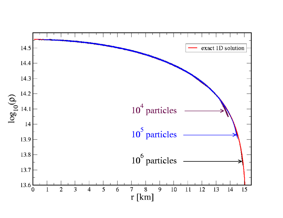
Figure 3: Density profile of a 1.4 M_⊙ neutron star. The solid red line is the result of solving the 1D stellar structure equations, the dots are the results obtained with the full SPH code at three different resolutions ($10^{4}$, $10^{5}$ and $10^{6}$ SPH particles).

As a test of the quality of the initial conditions we set up the particles in the described way, but instead of relaxing them, we evolve and monitor the kinetic energy that builds up as a result of small deviations from the true (numerical) hydrostatic equilibrium. We find only very minor differences resulting from the different particle setups. For very low particle numbers, say $1\,000$ particles, the gradients in the stellar profile cannot be resolved properly and the particles adjust their positions to find the equilibrium. For particle numbers in excess of $100\,000$ the particles smoothly move off the initial grid but the overall density structure is practically unperturbed.
Different particle masses are known to introduce numerical noise into SPH simulations. While a small range of particle masses may be admissible in some applications, we only use equal particle masses. As a numerical experiment, we set up a star with $10\,000$ particles and a constant particle number density, so that the particle masses carry the information of the stellar profile $\rho^{1D}(r)=nm(r)$. The extreme drop in density towards the neutron star surface (caused by the very stiff equation of state) translates for this particle setup in particle masses that vary by more than a factor of $10^{6}$. Without further relaxation we let this configuration evolve. This worst case setup results in spurious particle motions as very light particles are in direct contact with heavier particles in the neutron star interior. The slightest noise of the heavy particles strongly disturbs the light ones (“ping pong on cannon ball effect”) and leads to pathological particle densities, where low density particles can be found in the interior of the star. Therefore, we only use equal mass particles to keep the numerical noise at a minimal level.

3.2 Hydrodynamics

3.2.1 1D: Sod’s shock tube

Figure 4: Results of the Sod shock tube test in one dimension using 900 SPH particles setup using unsmoothed initial conditions. Artificial viscosity and thermal conductivity are applied to appropriately smooth the shock and contact discontinuity respectively. The exact solution is given by the solid line. The upper row displays the velocity (left) and the density (right), the bottom row shows specific internal energy (left) and the pressure (right).

As a standard test of the shock capturing capability we show the results of Sod’s shock tube test (Sod, 1978). To the left of the origin, the initial state of the fluid is given by [$\rho,P,v_{x}$]_L = [1.0,1.0,0.0] whilst to the right of the origin the initial state is [$\rho,P,v_{x}$]_R = [0.125,0.1,0.0] with $\gamma=1.4$. The problem is setup using 900 equal mass particles in one spatial dimension. Rather than adopting the usual practice of smoothing the initial conditions across the discontinuity, we follow Price (2004) in using unsmoothed initial conditions but applying a small amount of artificial thermal conductivity using the switch described in §2.2.3. The results are shown in Fig. 4, where the points represent the SPH particles. For comparison the exact solution computed using a Riemann solver is given by the solid line.
The shock itself is smoothed by the artificial viscosity term, which in this case can be seen to spread the discontinuity over about 5 smoothing lengths. The contact discontinuity is smoothed by the application of artificial thermal conductivity which (in particular) eliminates the “wall heating” effect often visible in numerical solutions to this problem. The exact distribution of particle separations in the contact discontinuity seen in Fig. 4 is related to the initial particle placement across the discontinuity.
For this test, applying artificial viscosity and thermal conductivity as described, we do not find a large difference between the “grad-$h$” formulation and other variants of SPH based on averages of the smoothing length. If anything, the “grad-$h$”-terms tend to increase the order of the method, which, as in any higher order scheme, tends to enhance oscillations which may otherwise be damped, visible in Fig. 4 as small “bumps” at the head of the rarefaction wave (in the absence of artificial viscosity these bumps appear as small but regular oscillations with a wavelength of a few particle spacings).

3.2.2 1D: The Einfeldt rarefaction test

Figure 5: Results of the Einfeldt test for the velocity (upper left), density (upper right), specific internal energy (lower left) and pressure (lower right). 400 particles were used in this test.

The initial conditions of the Einfeldt rarefaction test (Einfeldt et al., 1991) do not exhibit any discontinuity in density or pressure, but the two halfs of the computational domain move in opposite directions and thereby create a region of very low density near the initial velocity discontinuity. This low-density region represents a particular challenge for some iterative Riemann solvers which can return negative values for pressure/density. Einfeldt et al. (1991) designed a series of tests to illustrate this failure mode. The initial conditions of this test are [$\rho,P,v_{x}$]_L = [1.0,0.4,-2.0] for the left state and [$\rho,P,v_{x}$]_R = [1.0,0.4,2.0] for the right one. The results from a 400 particle calculation are shown in Fig. 5 after a time $t$= 0.2. The exact result is reproduced very accurately, only at the fronts of the rarefaction waves a small overshoot occurs. The low density region does not represent any problem for the method.

3.2.3 3D: Sedov blast wave test

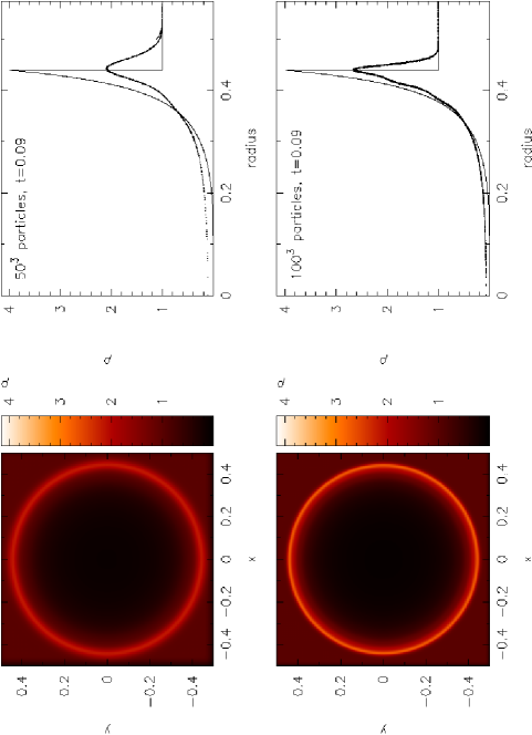
Figure 6: Results of the hydrodynamic Sedov blast wave test at $t=0.09$ at resolutions of $125\,000$ (top) and 1 million (bottom) particles respectively. The left panels show a rendered plot of the density in a slice taken at $z=0$ whilst the right panels show the density and radial position of each SPH particle, which may be compared to the exact solution given by the solid line. Note that we are showing each individual SPH particle and no averages.

In order to demonstrate that our scheme is capable of handling strong shocks in three dimensions, we have also tested the code on a Sedov blast wave problem both with, see Sec. 3.3.4, and without magnetic fields. Without magnetic fields the explosion is spherically symmetric, however for a strong magnetic field the blast wave is significantly inhibited perpendicular to the magnetic field lines, resulting in a compression along one spatial dimension. Similar tests for both hydrodynamics and MHD have been used by many authors – for example by Balsara (2001) in order to benchmark an Adaptive Mesh Refinement (AMR) code for MHD and by Springel & Hernquist (2002) to test a new formulation (entropy equation) of SPH.
The hydrodynamic version is set up as follows: The particles are placed in a cubic lattice configuration in a three dimensional domain $[-0.5,0.5]\times[-0.5,0.5]\times[-0.5,0.5]$ with uniform density $\rho=1$ and zero pressure and temperature apart from a small region $r<R$ near the origin, where we initialize the pressure using the total blast wave energy $E=1$, ie. $P=(\gamma-1)E/(\frac{4}{3}\pi R^{3})$. We set the initial blast radius to the size of a single particle’s smoothing sphere $R=2\eta\Delta x$ (where $2$ is the kernel radius, $\eta(=1.5)$ is the smoothing length in units of the average particle spacing as in Eq. (13) and $\Delta x$ is the initial particle spacing on the cubic lattice) such that the explosion is as close to point-like as resolution allows. Boundaries are not important for this problem, however we use periodic boundary conditions to ensure that the particle distribution remains smooth at the edges of the domain.
The results are shown in Fig. 6 at $t=0.09$. We have used a resolution of 50³ and 100³ particles (ie. $125\,000$ and 1 million particles respectively) and we have plotted (left panels) the density in a $z=0$ cross section slice and (right panels) the density and radial position of each particle (dots) together with the exact self-similar Sedov solution (solid line).
We found that the key to an accurate simulation of this problem in SPH is to incorporate an artificial thermal conductivity term due to the huge initial discontinuity in thermal energy. The importance of such a term for shock problems in SPH has been discussed recently by Price (2004). In the absence of this term the particle distribution quickly becomes disordered around the shock front and the radial profile appears to be noisy. From Fig. 6 we see that at a resolution of 1 million particles the highest density in the shock at $t=0.09$ is $\rho_{\rm max}=2.67$ whereas for the lower resolution run $\rho_{\rm max}=2.1$, consistent with a factor of 2 change in smoothing length. Using this we can estimate that a resolution of $\sim 345^{3}=41$ million particles is required to fully resolve the density jump in this problem in three dimensions. Note that the minimum density obtained in the post-shock rarefaction also decreases with resolution. Some small-amplitude post-shock oscillations are visible in the solution which we attribute to interaction of the spherical blast wave with particles in the surrounding medium initially placed on a regular (Cartesian) cubic lattice.

3.2.4 3D: Radial oscillation of a neutron star

As a further test case, we consider the radial oscillations of a neutron star using the Shen equation of state (Shen et al., 1998a, b). The initial conditions are a neutron star relaxed into hydrostatic equilibrium as described previously (§3.1), given an initial perturbation in velocity of the form ${\bf v}=v_{0}\hat{\bf r}$ where $v_{0}$ is an arbitrary but small amplitude (we choose $v_{0}=0.01$c). No artificial viscosity or damping is applied for this problem since no shocks are involved. We compute the problem at low resolution using only $10\,000$ particles in the neutron star.
The results of this test are given in Fig. 7, which shows the results of an integration for 10 oscillation periods, where top and bottom panels show the total and gravitational potential energy respectively. From this Figure it may be observed that the amplitude is maintained almost exactly by the code over the 10 oscillation periods ($P\approx 0.33$ ms) simulated. The residual fluctuations in total energy are directly attributable to a combination of the tree opening criterion (here $\theta=0.9$), which we find controls the level of “noise” in the total energy curve, and the timestepping accuracy (Courant number, here $C_{\rm cour}=0.2$), which affects the mean curve.
The fact that our SPH code, even at low resolution, is capable of following the neutron star oscillations for many periods without significant damping suggests that the code may be an ideal tool for studying neutron star oscillation modes. A similar study has recently been performed by Monaghan & Price (2006) who compared SPH simulations of the oscillation modes of two dimensional “Toy stars” (Monaghan & Price, 2004) with exact and perturbation solutions, finding good agreement between the two.

3.2.5 3D: Binary orbit

Figure 7: Total (top) and gravitational potential energy (bottom) for 10 radial oscillations of an initially hydrostatic neutron star using the Shen equation of state.

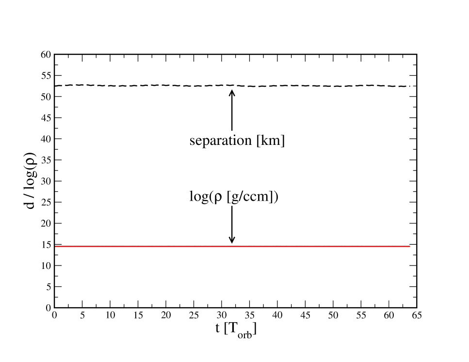
Figure 8: Evolution of a neutron star binary system set on a circular orbit with a initial separation of $a_{0}=52.5$ km. Displayed are the orbital separation (upper line) and the maximum matter density (lower line). The binary system is evolved for as long as 63 orbital periods or about 920 neutron star dynamical time scales.

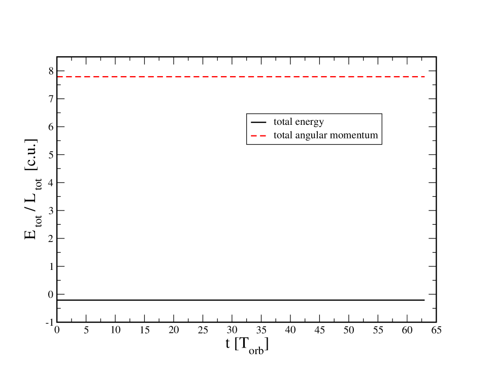
Figure 9: Evolution of total energy and angular momentum (both in code units) during the orbital revolution of a binary system with twice 1.4 M_⊙.

As a further test in 3D we set up a neutron star binary system on a stable circular orbit and follow its long-term evolution. As initial separation we choose $a_{0}=52.5$ km (= 35 code units), no gravitational backreaction forces are applied. To demonstrate that even at a very low resolution stable and accurate orbital evolution can be obtained, we model each neutron star with $1\,300$ SPH particles only. We relax two neutron stars in a corotating frame as described in Rosswog et al. (2004). After a tidally locked equilibrium configuration has been reached, the velocities are transformed to the space-fixed frame and the orbital evolution is followed with the full code for as long as 63 orbital periods or approximately 920 dynamical time scales of the neutron stars. The evolution of the orbital separation of both neutron stars together with the maximum density in the binary system are shown in Fig. 8. The binary stays nearly perfectly on the intended orbit. Due to the finite relaxation time very small scale oscillations occur which lead to an exchange between orbital and oscillation energy of the stars. This leads to small oscillations of the orbital separation around the initial value. But the corresponding deviations are very small ($\delta a_{\rm max}/a_{0}\approx 0.005$) and they do not grow during the very long evolution time. The central density is free of any visible oscillation.
The evolution of the corresponding total energy, $E_{\rm tot}$, and the total angular momentum, $L_{\rm tot}$, are shown in Fig. 9. Both quantities are excellently conserved: $\delta E_{\rm tot}/E_{\rm tot,0}<10^{-3}$ and $\delta L_{\rm tot}/L_{\rm tot,0}<10^{-4}$.

3.2.6 3D: Stellar head-on collision

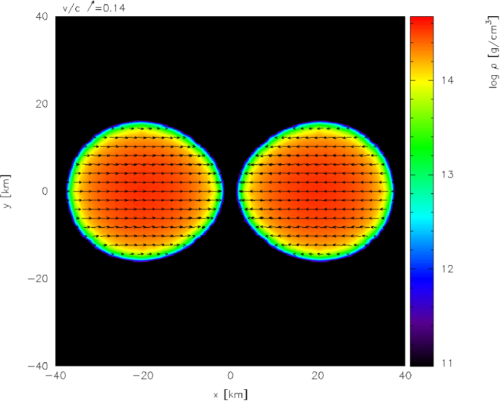
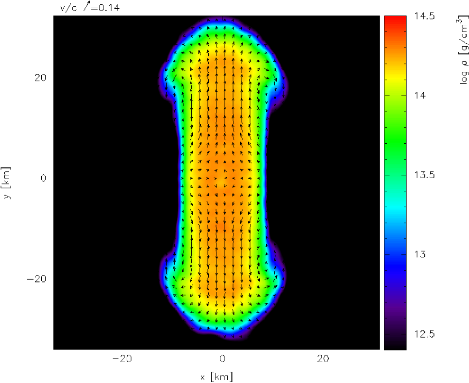
Figure 10: Head-on collision of two neutron stars. Such a head-on collision of two stars is considered a worst-case situation for the non-conservation of energy due to changes in the smoothing lengths, see text for details.

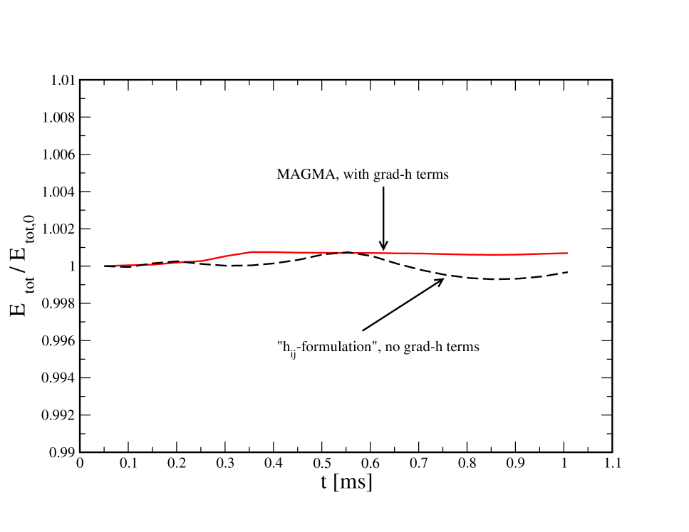
Figure 11: Comparison of the energy conservation of both SPH-formulations (see text for details) for the above head-on collision. Both formulations yield very good conservation properties. The dominant error sources are the tree opening criterion and the time stepping criterion. To see a difference from the grad-h-terms, the tree opening criterion had to be reduced to $\theta=0.1$ and the pre-factor in Eq. 67 to 0.1.

It has long been known (Hernquist, 1993) that using the SPH equations derived under the assumption of constant smoothing lengths, e.g. in the conventional $h_{ij}$-formulation summarized in Sec. 2.2.1, but still allowing the smoothing lengths to change in practice, can in extreme cases lead to substantial errors in the conservation of energy. For example, Hernquist (1993) found a non-conservation of energy on a $\sim 10$-%-level for a violent head-on collision of two polytropic stars. To quantify this non-conservation for MAGMA we perform a similar head-on collision between two neutron stars. Two neutron stars ($35\,000$ particles each) of 1.4 M_⊙ obeying the Shen et al. (1998b) equation of state are set to an initial separation of 35 code units (=52.5 km) and provided with an initial relative velocity of 0.1 c. Fig. 10 shows two density snapshots with overlaid velocity field during the evolution.
In Fig.11 we show the evolution of the total energy both for the $h_{ij}$-formulation and the new “grad-$h$”-version (both are normalized to their initial values). As in previous work (Rosswog & Davies, 2002; Rosswog & Liebendörfer, 2003; Rosswog et al., 2003) we use on average 100 neighbors for the $h_{ij}$-formulation, for the “grad-$h$”-version we use a constant of $\eta=1.5$ in Eq. (13).
Generally the energy is very well conserved in both cases and the non-conservation is determined by the tree-opening criterion and the time stepping accuracy. To see a difference between both formulations, we reduced the tree opening criterion to $\theta=0.1$ and the pre-factor in Eq. (67) to 0.1. Both codes conserve energy in this challenging problem to better than about $10^{-3}$ with the “grad-$h$”-version showing a slightly better performance. As in the other tests presented here, wee see a small improvement, but no major change due to the use of the grad-$h$-terms.

3.3 Magnetohydrodynamics

3.3.1 1D: Brio-Wu shock tube test

Figure 12: Results of the Brio & Wu MHD shock tube test at $t=0.1$ using 631 particles and the Euler potential formulation. For comparison the numerical solution taken from Balsara (1998) is given by the solid line. The solution illustrates the complex shock structures which can be formed due to the different wave types in MHD, including in this case a compound wave consisting of a slow shock attached to a rarefaction wave.

The magnetic shock tube test of Brio & Wu (1988) has become a standard test case for numerical MHD schemes that has been widely used by many authors to benchmark (mainly grid-based) MHD codes (e.g. Stone et al., 1992; Dai & Woodward, 1994; Ryu & Jones, 1995; Balsara, 1998). The Brio-Wu shock test is the MHD analogon to Sod’s shock tube problem that was described in Sec. 3.2.1, but here no analytical solution is known. The MHD Riemann problem allows for much more complex solutions than the hydrodynamic case which can occur because of the three different types of waves (i.e. slow, fast and Alfvén, compared to just the sound waves in hydrodynamics). In the Brio-Wu shock test the solution contains the following components (from left to right in Fig. 12): a fast rarefaction fan and a slow compound wave consisting of a slow rarefaction attached to a slow shock (moving to the left) and a contact discontinuity, a slow shock and a fast rarefaction fan (moving to the right). It has been pointed out, however, that the stability of the unusual compound wave may be an artifact of the restriction of the symmetry to one spatial dimension whilst allowing the magnetic field to vary in two dimensions (Barmin et al., 1996).
Here we present the first results using the Euler potential formulation, see §2.3.4. Results of this problem using Smoothed Particle Magnetohydrodynamics (SPMHD) have been presented by Price & Monaghan (2004a) and Price (2004). The Euler potentials show a distinct improvement over the standard SPMHD results. The initial conditions on the left side of the discontinuity are $[\rho,P,v_{x},v_{y},B_{y}]_{\rm L}=[1,1,0,0,1]$ and $[\rho,P,v_{x},v_{y},B_{y}]_{\rm R}=[0.125,0.1,0,0,-1]$ on the right side. The $x-$component of the magnetic field is $B_{x}=0.75$ everywhere and a polytropic exponent of $\gamma=2.0$ is used. Using the Euler potentials the components are given by $\alpha=-B_{y}x$ (equivalent to the vector potential $A_{z}$) and $\beta=z$ (or more specifically $\nabla\beta=\hat{\bf z}$) and the $B_{x}$ component is treated as an external field which requires adding a source term to the evolution equation for $\alpha$ as discussed in §2.3.4. Particles are restricted to move in one spatial dimension only, whilst the magnetic field is allowed to vary in two dimensions (that is, we compute a $v_{y}$ but do not use it to move the particles). This is sometimes referred to as a “1.5D” approximation.
We setup the problem using 631 equal mass particles in the domain $x\in[-0.5,0.5]$ using, as in the hydrodynamic case, purely discontinuous initial conditions. Artificial viscosity, thermal conductivity and resistivity are applied as described in §2.2.3 and §2.3.4. The results are shown at $t=0.1$ in Fig. 12. For comparison the numerical solution from Balsara (1998) is given by the solid line (no exact solution exists for this problem). The solution is generally well captured by our numerical scheme. Two small defects are worth noting. The first is that a small offset is visible in the thermal energy – this is a result of the small non-conservation introduced by use of the Morris formulation of the magnetic force (required for stability, see Eq. (45)). Secondly, the rightmost discontinuity is somewhat over-smoothed by the artificial resistivity term. We attribute this to the fact that the dissipative terms involve simply the maximum signal velocity $v_{sig}$ (that is the maximum of all the wave types). Ideally each discontinuity should be smoothed taking account of its individual characteristic and corresponding $v_{sig}$ (as would occur in a Godunov-MHD scheme). Increasing the total number of particles also decreases the smoothing applied to this wave.

3.3.2 2D: Current loop advection problem

A simple test problem for MHD is to compute the advection of a weak magnetic field loop. This test, introduced by Gardiner & Stone (2005) in the development of the Athena MHD code, presents a challenging problem for grid-based MHD schemes requiring careful formulation of the advection terms in the MHD equations. For our Lagrangian scheme, this test is straightforward to solve which strongly highlights the advantage of using a particle method for MHD in problems where there is significant motion with respect to a fixed reference frame.
We setup the problem here following Gardiner & Stone (2005): The computational domain is two dimensional with $x\in[-1,1]$, $y\in[-0.5,0.5]$ using periodic boundary conditions. Density and pressure are uniform with $\rho=1$ and $P=1$. The particles are laid down in a cubic lattice configuration with velocity initialized according to ${\bf v}=(v_{0}\cos{\theta},v_{0}\sin{\theta})$ with $\cos{\theta}=2/\sqrt{5}$, $\sin{\theta}=1/\sqrt{5}$ and $v_{0}=1$ such that by $t=1$ the field loop will have been advected around the computational domain once. The magnetic field is two dimensional, initialized using a vector potential given by

$$A_{z}=\alpha=\left\{\begin{array}[]{ll}A_{0}(R-r)&r\leq R,\\ 0&r>R,\end{array}\right.$$ (68)

where $A_{0}=10^{-3}$, $R=0.3$ and $r=\sqrt{x^{2}+y^{2}}$. The ratio of thermal to magnetic pressure is thus given by $\beta_{\rm plas}=P/(\frac{1}{2}B^{2})=2\times 10^{6}$ (for $r<R$) such that the magnetic field is passively advected.

Figure 13: Magnetic field lines in the current loop advection test, plotted at $t=0$ (top) and after $1\,000$ crossings of the computational domain (bottom).

Gardiner & Stone (2005) show the results of this problem after two crossings of the computational domain, by which time the loop has either been significantly diffused or has disintegrated into oscillations depending on details of their particular choice of scheme. The advantage of a Lagrangian scheme is that advection is computed exactly, and using our Euler potential formulation (which in two dimensions is equivalent to a vector potential formulation with $\alpha=A_{z}$ and $\beta=z$) for the magnetic field, this is also true for the evolution of the magnetic field. The result is that the field loop is advected without change by our code for as long as one may care to compute it. This is demonstrated in Fig. 13 which shows the magnetic field lines at $t=0$ (top) and after $1\,000$ (this is not a misprint!) crossings of the computational domain (bottom), in which the field configuration can be seen to be identical to the top figure. The magnetic energy (not shown) is also maintained exactly, whereas Gardiner & Stone (2005) find of order a 10% reduction in magnetic energy after two crossings of the domain.
In a realistic simulation involving MHD shocks there will be some diffusion of the magnetic field introduced by the addition of artificial diffusion terms, see Eq. (63), which are required to resolve discontinuities in the magnetic field. However the point is that these terms are explicitly added to the SPH calculation and can be turned off where they are not necessary (for example using the switches described in §2.2.3 and §2.3.2) whereas the diffusion present in a grid-based code is intrinsic and always present.

3.3.3 2D: Orszag-Tang test

The evolution of the compressible Orszag-Tang vortex system (Orszag & Tang, 1979) involves the interaction of several shock waves traveling at different speeds. Originally studied in the context of incompressible MHD turbulence, it has later been extended to the compressible case (Dahlburg & Picone, 1989; Picone & Dahlburg, 1991). It is generally considered a good test to validate the robustness of numerical MHD schemes and has been used by many authors (e.g. Ryu & Jones, 1995; Dai & Woodward, 1998; Jiang & Wu, 1999; Londrillo & Del Zanna, 2000). In the SPH context, this test has been discussed in detail by Price (2004) and Price & Monaghan (2005).
The problem is two dimensional with periodic boundary conditions on the domain $[0,1]\times[0,1]$. The setup consists of an initially uniform state perturbed by periodic vortices in the velocity field, which, combined with a doubly periodic field geometry, results in a complex interaction between the shocks and the magnetic field.
The velocity field is given by $\vec{v}=v_{0}[-\sin{(2\pi y)},\sin{(2\pi x)}]$ where $v_{0}=1$. The magnetic field is given by $\vec{B}=B_{0}[-\sin{(2\pi y)},\sin{(4\pi x)}]$ where $B_{0}=1/\sqrt{4\pi}$. Using the Euler potentials this corresponds to $\alpha\equiv A_{z}=B_{0}/(2\pi)[\cos{(2\pi y)}+\frac{1}{2}\cos{(4\pi x)}]$. The flow has an initial average Mach number of unity, a ratio of magnetic to thermal pressure of $10/3$ and we use a polytropic exponent $\gamma=5/3$. The initial gas state is therefore $P=5/3B_{0}^{2}=5/(12\pi)$ and $\rho=\gamma P/v_{0}=25/(36\pi)$. Note that the choice of length and time scales differs slightly between various implementations in the literature. The setup used above follows that of Ryu & Jones (1995) and Londrillo & Del Zanna (2000).
We compute the problem using $512\times 590$ particles initially placed on a uniform, close-packed lattice. The density at $t=0.5$ is shown in Fig. 14 using both the standard SPMHD formalism (left), see §2.3.1, and the Euler potential formalism (right), see §2.3.3. The Euler potential formulation is clearly superior to the standard SPMHD method. This is largely a result of the relative requirements for artificial resistivity in each case. In the standard SPMHD method the application of artificial resistivity is crucial for this problem (that is, in the absence of artificial resistivity the density and magnetic field distributions are significantly in error). Using the Euler potentials we find that the solution can be computed using zero artificial resistivity, relying only on the “implicit smoothing” present in the computation of the magnetic field using SPH operators in Eqs. (59) and (60). This means that topological features in the magnetic field are much better preserved, which is reflected in the density distribution. For example the filament near the center of the figure is well resolved using the Euler potentials but completely washed out by the artificial resistivity in the standard SPMHD formalism. Also the high density features near the top and bottom of the figure (coincident to a reversal in the magnetic field) are much better resolved using the Euler potentials.
A further advantage of using the Euler potentials is that the field lines can be plotted directly as equipotential surfaces of the potentials. The field lines corresponding to Fig. 14 are thus shown in Fig. 16.
In order to enable a comparison between different codes, we also show the 1D pressure distribution along the lines $y=0.4277$ and $y=0.3125$ in Fig. 15 which may be compared to similar plots given in Fig. 11 of Londrillo & Del Zanna (2000) and in Jiang & Wu (1999).

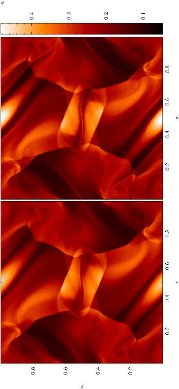
Figure 14: Density distribution in the two dimensional Orzsag-Tang vortex problem at $t=0.5$. The initial vortices in the velocity field combined with a doubly periodic field geometry lead to a complex interaction between propagating shocks and the magnetic field. Results are shown using $512\times 590$ particles using a standard SPMHD formalism (left) and using the Euler potentials (right). The reduced artificial resistivity required in the Euler potential formalism leads to a much improved effective resolution. The plot may be compared to results shown at comparable resolution in Fig. 14 of Dai & Woodward (1998).

Figure 15: Pressure distribution in the Orzsag-Tang vortex problem (as in Fig. 14) along a 1D cut taken at $y=0.4277$ (upper panel) and $y=0.3125$ (lower panel). The plots can be compared to Fig. 11 in Londrillo & Del Zanna (2000), see also Jiang & Wu (1999).

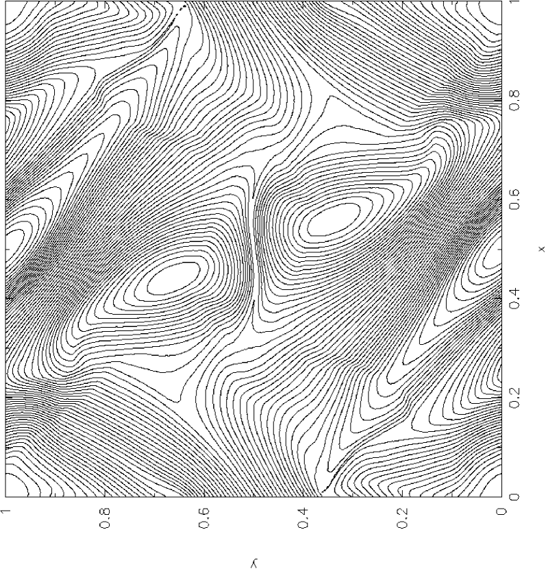
Figure 16: Magnetic field lines (contours of the Euler potential $\alpha$) in the two dimensional Orszag-Tang vortex problem at $t=0.5$ (corresponding to the right panel of Fig. 14). This may be compared to Fig. 15 in Dai & Woodward (1998) and Fig. 10 in Londrillo & Del Zanna (2000).

3.3.4 3D: MHD blast wave

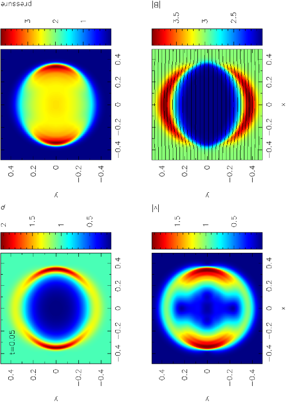
Figure 17: Results of the MHD blast wave test at $t=0.05$ at a resolution of 1 million ($100^{3}$) particles. Plots show (left to right, top to bottom) density, pressure, magnitude of velocity and magnetic field strength (with overlaid field lines), plotted in a cross-section slice through the $z=0$ plane.

There appear to be very few three dimensional MHD solutions published in the literature. Here we perform an MHD version of the Sedov test, identical to the hydrodynamic test with the addition of a uniform magnetic field in the $x-$ direction, that is ${\bf B}=[B_{0},0,0]$ with $B_{0}=3.0$. A similar test has been used by Balsara (2001) for testing a 3D Adaptive Mesh Refinement code although with weak magnetic fields. Here we perform the test in the strong field regime such that the geometry of the blast is significantly constrained by the magnetic field, testing both the magnetic field evolution and the formulation of magnetic forces in the code. Initially the surrounding material has zero thermal pressure, meaning that the plasma $\beta_{\rm plas}$ is zero (ie. magnetic pressure infinitely strong compared to thermal pressure). However, this choice of field strength gives a mean plasma $\beta_{\rm plas}$ in the post-shock material of $\beta_{\rm plas}\sim 1.3$, such that the magnetic pressure plays an equal or dominant role in the evolution of the shock.
The initial Euler potentials for the blast wave are:

$$\alpha=-B_{0}z\quad{\rm and}\quad\beta=y$$ (69)

where an offset is applied to each potential at the boundaries to ensure periodicity.
The results of this problem at $t=0.05$ are shown in Fig. 17, where plots show density, pressure, magnitude of velocity and magnetic field strength in a cross section slice taken at $z=0$. In addition the magnetic field lines are plotted on the magnetic field strength plot.
In this strong-field regime, the magnetic field lines are not significantly bent by the propagating blast wave but rather strongly constrain the blast wave into an oblate spheroidal shape. The density (and likewise pressure) enhancement in the shock is significantly reduced in the $y-$direction (left and top right panels) due to the additional pressure provided by the magnetic field which is compressed in this direction (bottom right panel).

4 Summary and Outlook

We have introduced a new, 3D code, MAGMA, for astrophysical magnetohydrodynamic problems that is based on the smoothed particle hydrodynamics method. The equations of self-gravitating hydrodynamics are derived self-consistently from a Lagrangian and account in particular for the so-called “grad-h”-terms. Contrary to other approaches, we also account for the extra terms in the gravitational acceleration terms that stem from changes in the smoothing length. This part of the code has been extensively tested on a large set of standard test problems. The code performs very well, in particular its conservation properties are excellent. While the “grad-h”-terms slightly improve the accuracy, in typical applications involving neutron stars the differences to the older set of equations are very minor.
We evolve the magnetic fields with so-called Euler potentials which are advected on the SPH-particles. They correspond to a formulation of the magnetic field in terms of a vector potential, therefore, the $\nabla\cdot\vec{B}=0$ constraint is satisfied by construction. To handle strong shocks artificial dissipative terms were introduced in these potentials, but for several tests no artificial dissipation is required and the corresponding terms can be switched off. The Euler potential approach shows in all tests a considerably higher accuracy than previous magnetic SPH formulations and is our method of choice for our future astrophysical applications of the MAGMA code.

References

- Akiyama et al. (2003) Akiyama S., Wheeler J. C., Meier D. L., Lichtenstadt I., 2003, ApJ, 584, 954
- Ardeljan et al. (2005) Ardeljan N. V., Bisnovatyi-Kogan G. S., Moiseenko S. G., 2005, MNRAS, 359, 333
- Balbus & Hawley (1998) Balbus S. A., Hawley J. F., 1998, Reviews of Modern Physics, 70, 1
- Balsara (1995) Balsara D., 1995, J. Comput. Phys., 121, 357
- Balsara (1998) Balsara D. S., 1998, ApJS, 116, 133
- Balsara (2001) Balsara D. S., 2001, J. Comp. Phys., 174, 614
- Banerjee & Pudritz (2006) Banerjee R., Pudritz R. E., 2006, ArXiv Astrophysics e-prints
- Barmin et al. (1996) Barmin A. A., Kulikovskiy A. G., Pogorelov N. V., 1996, J. Comp. Phys., 126, 77
- Benz (1990) Benz W., 1990, in Buchler J., ed., , Numerical Modeling of Stellar Pulsations. Kluwer Academic Publishers, Dordrecht, p. 269
- Benz et al. (1990) Benz W., Bowers R., Cameron A., Press W., 1990, ApJ, 348, 647
- Bisnovatyi-Kogan et al. (1976) Bisnovatyi-Kogan G. S., Popov Y. P., Samochin A. A., 1976, Astrophysics and Space Science, 41, 321
- Børve et al. (2001) Børve S., Omang M., Trulsen J., 2001, ApJ, 561, 82
- Børve et al. (2004) Børve S., Omang M., Trulsen J., 2004, ApJS, 153, 447
- Brio & Wu (1988) Brio M., Wu C. C., 1988, Journal of Computational Physics, 75, 400
- Brookshaw (1985) Brookshaw L., 1985, Proceedings of the Astronomical Society of Australia, 6, 207
- Burrows et al. (2007) Burrows A., Dessart L., Livne E., Ott C. D., Murphy J., 2007, ArXiv Astrophysics e-prints
- Dahlburg & Picone (1989) Dahlburg R. B., Picone J. M., 1989, Physics of Fluids B, 1, 2153
- Dai & Woodward (1994) Dai W., Woodward P. R., 1994, J. Comp. Phys., 115, 485
- Dai & Woodward (1998) Dai W., Woodward P. R., 1998, ApJ, 494, 317
- De Villiers et al. (2003) De Villiers J.-P., Hawley J. F., Krolik J. H., 2003, ApJ, 599, 1238
- Dolag et al. (2002) Dolag K., Bartelmann M., Lesch H., 2002, A&A, 387, 383
- Duez et al. (2006) Duez M. D., Liu Y. T., Shapiro S. L., Shibata M., Stephens B. C., 2006, Physical Review Letters, 96, 031101
- Duez et al. (2007) Duez M. D., Liu Y. T., Shapiro S. L., Shibata M., Stephens B. C., 2007, ArXiv General Relativity and Quantum Cosmology e-prints
- Eckart (1960) Eckart C., 1960, Physics of Fluids, 3, 421
- Einfeldt et al. (1991) Einfeldt B., Roe P. L., Munz C. D., Sjogreen B., 1991, Journal of Computational Physics, 92, 273
- Español & Revenga (2003) Español P., Revenga M., 2003, Phys. Rev. E, 67, 026705
- Euler (1769) Euler L., 1769, Novi Commentarrii Acad. Sci. Petropolitanae, 14, 270
- Fromang & Nelson (2006) Fromang S., Nelson R. P., 2006, A&A, 457, 343
- Gardiner & Stone (2005) Gardiner T. A., Stone J. M., 2005, J. Comp. Phys., 205, 509
- Gingold & Monaghan (1977) Gingold R. A., Monaghan J. J., 1977, MNRAS, 181, 375
- Hawley & Krolik (2006) Hawley J. F., Krolik J. H., 2006, ApJ, 641, 103
- Hernquist (1993) Hernquist L., 1993, ApJ, 404, 717
- Hosking & Whitworth (2004) Hosking J. G., Whitworth A. P., 2004, MNRAS, 347, 1001
- Jiang & Wu (1999) Jiang G.-S., Wu C.-C., 1999, Journal of Computational Physics, 150, 561
- Kotake et al. (2004) Kotake K., Sawai H., Yamada S., Sato K., 2004, ApJ, 608, 391
- LeBlanc & Wilson (1970) LeBlanc J. M., Wilson J. R., 1970, ApJ, 161, 541
- Liebendörfer et al. (2004) Liebendörfer M., Pen U., Thompson C., 2004, astro-ph/0408161
- Lomax et al. (2001) Lomax H., Pulliam T., Zingg D., 2001, Fundamentals of Computational Fluid Dynamics. Springer, Berlin
- Londrillo & Del Zanna (2000) Londrillo P., Del Zanna L., 2000, ApJ, 530, 508
- Machida et al. (2006) Machida M. N., Matsumoto T., Hanawa T., Tomisaka K., 2006, ApJ, 645, 1227
- Masada et al. (2006) Masada Y., Sano T., Takabe H., 2006, ApJ, 641, 447
- McKinney (2005) McKinney J. C., 2005, ArXiv Astrophysics e-prints
- McKinney & Narayan (2007) McKinney J. C., Narayan R., 2007, MNRAS, pp 1495–+
- Meier et al. (1976) Meier D. L., Epstein R. I., Arnett W. D., Schramm D. N., 1976, ApJ, 204, 869
- Mizuno et al. (2004) Mizuno Y., Yamada S., Koide S., Shibata K., 2004, ApJ, 615, 389
- Monaghan (1992) Monaghan J., 1992, Ann. Rev. Astron. Astrophys., 30, 543
- Monaghan & Lattanzio (1985) Monaghan J., Lattanzio J., 1985, A&A, 149, 135
- Monaghan (1997) Monaghan J. J., 1997, Journal of Computational Physics, 136, 298
- Monaghan (2002) Monaghan J. J., 2002, MNRAS, 335, 843
- Monaghan (2005) Monaghan J. J., 2005, Reports of Progress in Physics, 68, 1703
- Monaghan & Price (2004) Monaghan J. J., Price D. J., 2004, MNRAS, 350, 1449
- Monaghan & Price (2006) Monaghan J. J., Price D. J., 2006, MNRAS, 365, 991
- Morris & Monaghan (1997) Morris J., Monaghan J., 1997, J. Comp. Phys., 136, 41
- Morris (1996a) Morris J. P., 1996a, Publications of the Astronomical Society of Australia, 13, 97
- Morris (1996b) Morris J. P., 1996b, PhD thesis, Monash University, Melbourne, Australia
- Nelson & Papaloizou (1994) Nelson R., Papaloizou J., 1994, MNRAS, 270, 1
- Nelson (2005) Nelson R. P., 2005, A&A, 443, 1067
- Obergaulinger et al. (2006) Obergaulinger M., Aloy M. A., Müller E., 2006, A&A, 450, 1107
- Orszag & Tang (1979) Orszag S., Tang C., 1979, Journ. Fluid Mech., 90, 129
- Phillips & Monaghan (1985) Phillips G. J., Monaghan J. J., 1985, MNRAS, 216, 883
- Picone & Dahlburg (1991) Picone J. M., Dahlburg R. B., 1991, Physics of Fluids B, 3, 29
- Price (2004) Price D., 2004, PhD thesis, University of Cambridge, arXiv:astro-ph/0507472
- Price & Monaghan (2007) Price D., Monaghan J., 2007, MNRAS, 374, 1347
- Price & Rosswog (2006) Price D., Rosswog S., 2006, Science, 312, 719
- Price & Bate (2007a) Price D. J., Bate M. R., 2007a, arXiv:0705.1096, 705
- Price & Bate (2007b) Price D. J., Bate M. R., 2007b, MNRAS, 377, 77
- Price & Monaghan (2004a) Price D. J., Monaghan J. J., 2004a, MNRAS, 348, 123
- Price & Monaghan (2004b) Price D. J., Monaghan J. J., 2004b, MNRAS, 348, 139
- Price & Monaghan (2005) Price D. J., Monaghan J. J., 2005, MNRAS, 364, 384
- Proga (2005) Proga D., 2005, ApJ, 629, 397
- Rosswog (2005) Rosswog S., 2005, ApJ, 634, 1202
- Rosswog & Davies (2002) Rosswog S., Davies M. B., 2002, MNRAS, 334, 481
- Rosswog et al. (2000) Rosswog S., Davies M. B., Thielemann F.-K., Piran T., 2000, A&A, 360, 171
- Rosswog & Liebendörfer (2003) Rosswog S., Liebendörfer M., 2003, MNRAS, 342, 673
- Rosswog et al. (2003) Rosswog S., Ramirez-Ruiz E., Davies M. B., 2003, MNRAS, 345, 1077
- Rosswog et al. (2004) Rosswog S., Speith R., Wynn G. A., 2004, MNRAS, 351, 1121
- Ryu & Jones (1995) Ryu D., Jones T. W., 1995, ApJ, 442, 228
- Sano et al. (2004) Sano T., Inutsuka S.-i., Turner N. J., Stone J. M., 2004, ApJ, 605, 321
- Shen et al. (1998a) Shen H., Toki H., Oyamatsu K., Sumiyoshi K., 1998a, Nuclear Physics, A 637, 435
- Shen et al. (1998b) Shen H., Toki H., Oyamatsu K., Sumiyoshi K., 1998b, Progress of Theoretical Physics, 100, 1013
- Shibata et al. (2006) Shibata M., Duez M. D., Liu Y. T., Shapiro S. L., Stephens B. C., 2006, Physical Review Letters, 96, 031102
- Shibata et al. (2006) Shibata M., Liu Y. T., Shapiro S. L., Stephens B. C., 2006, Phys. Rev. D, 74, 104026
- Sod (1978) Sod G., 1978, J. Comput. Phys., 43, 1
- Springel & Hernquist (2002) Springel V., Hernquist L., 2002, MNRAS, 333, 649
- Stern (1970) Stern D., 1970, American Journal of Physics, 38, 494
- Stern (1994) Stern D., 1994, Journal of geophysical research, 99, 17169
- Stern (1966) Stern D. P., 1966, Space Science Reviews, 6, 147
- Stone et al. (1992) Stone J. M., Hawley J. F., Evans C. R., Norman M. L., 1992, ApJ, 388, 415
- Stone & Pringle (2001) Stone J. M., Pringle J., 2001, MNRAS, 322, 461
- Symbalisty (1984) Symbalisty E. M. D., 1984, ApJ, 285, 729
- Watkins et al. (1996) Watkins S., Bhattal A., Francis N., Turner J., Whitworth A., 1996, A&AS, 119, 177
- Yamada & Sawai (2004) Yamada S., Sawai H., 2004, ApJ, 608, 907
- Ziegler (2005) Ziegler U., 2005, A&A, 435, 385