Resumen

We classify the entire minimal vertical graphs in the Heisenberg group ${\rm Nil_{3}}$ endowed with a Riemannian left-invariant metric. This classification, which provides a solution to the Bernstein problem in ${\rm Nil}_{3}$, is given in terms of the Abresch-Rosenberg holomorphic differential for minimal surfaces in ${\rm Nil}_{3}$.

1 Introduction

A recent major achievement in the theory of constant mean curvature (CMC) surfaces in Riemannian $3$-manifolds has been the discovery by Abresch and Rosenberg [AbRo1, AbRo2] of a holomorphic quadratic differential for every CMC surface in any homogeneous $3$-manifold with a $4$-dimensional isometry group. The most remarkable consequence of this construction is the classification given in [AbRo1, AbRo2] of the immersed CMC spheres in these homogeneous spaces as embedded rotational ones, thus solving an open problem proposed in [HsHs].

Our purpose in this paper is to solve by means of the Abresch-Rosenberg differential another popular open problem in the theory of CMC surfaces in homogeneous spaces. Namely, the Bernstein problem in the Riemannian Heisenberg $3$-space ${\rm{Nil}_{3}}$, i.e. the classification of the entire minimal vertical graphs in ${\rm{Nil}_{3}}$.

Let us fix some terminology. By using exponential coordinates and up to re-scaling, we shall regard the Heisenberg space ${\rm{Nil}_{3}}$ as $\mathbb{R}^{3}$ endowed with the Riemannian metric

$$d\sigma^{2}:=dx^{2}+dy^{2}+\left(dz+\frac{1}{2}(ydx-xdy)\right)^{2}\mathchar 46\relax$$

This Riemannian metric is left-invariant for the Lie group structure of Heisenberg space. In this way ${\rm{Nil}_{3}}$ becomes one of the five simply-connected canonical homogeneous $3$-manifolds with a $4$-dimensional isometry group.

A (vertical) graph $z=f(x,y)$ in ${\rm{Nil}_{3}}$ is said to be minimal if its mean curvature vanishes identically, and entire if it is defined for every $(x,y)\in\mathbb{R}^{2}$. The Bernstein problem in ${\rm{Nil}_{3}}$ asks for the classification of all entire vertical minimal graphs of ${\rm{Nil}_{3}}$. Equivalently, we wish to find all the $C^{2}$ solutions globally defined on $\mathbb{R}^{2}$ of the quasilinear elliptic PDE

$$(1+\beta^{2})f_{xx}-2\alpha\beta\,f_{xy}+(1+\alpha^{2})f_{yy}=0,$$ (1.1)

where $\alpha:=f_{x}+y/2$ and $\beta:=f_{y}-x/2$ (see [ADR, IKOS] for instance).

The simplest entire solutions to (1.1) are the linear ones, which give rise to entire minimal graphs in ${\rm{Nil}_{3}}$ that are called horizontal umbrellas [AbRo2]. In this model they are just non-vertical planes, but they are not totally geodesic. Other simple solution is $f(x,y)=xy/2$, and more generally, the $1$-parameter family [FMP]

$$f(x,y)=\frac{xy}{2}-c\left(y\sqrt{1+y^{2}}+\log\left(y+\sqrt{1+y^{2}}\right)\right),\hskip 22.76228ptc\in\mathbb{R}\mathchar 46\relax$$ (1.2)

The resulting entire minimal graphs are called saddle-type minimal examples [AbRo2]. There are other explicit entire solutions to (1.1) foliated by Euclidean straight lines (see [Dan2]), what suggests that the class of entire minimal graphs in ${\rm{Nil}_{3}}$ is quite large.

The Bernstein problem in ${\rm{Nil}_{3}}$ is a usual discussion topic among people working on CMC surfaces in homogeneous spaces, and appears explicitly as an open problem in several works like [FMP, AbRo2, Dan2, IKOS, MMP]. Let us also point out that the Bernstein problem in the sub-Riemannian Heisenberg space $\mathbb{H}^{1}$ has been intensely studied in the last few years (see [BSV, CHMY, GaPa, RiRo] and references therein).

In this work we show that the moduli space of entire minimal graphs in ${\rm{Nil}_{3}}$ can be parametrized in terms of their Abresch-Rosenberg differentials. Specifically, we prove:

Theorem 1 (Main Theorem)

Let $Qdz^{2}$ be a holomorphic quadratic differential in $\Sigma\equiv\mathbb{C}$ or $\mathbb{D}$ which is not identically zero if $\Sigma\equiv\mathbb{C}$. Then there exists a $2$-parameter family of (generically non-congruent) entire minimal graphs in ${\rm{Nil}_{3}}$ whose Abresch-Rosenberg differential is $Qdz^{2}$.

Conversely, any entire minimal graph in ${\rm{Nil}_{3}}$ is one of the above examples.

It is worth mentioning that if two holomorphic quadratic differentials on $\mathbb{C}$ or $\mathbb{D}$ only differ by a global conformal change of parameter, then the families of minimal graphs that they induce are the same (the corresponding immersions differ by this conformal global change of parameter).

We also remark that the conformally immersed minimal surfaces $X:\Sigma\rightarrow{\rm{Nil}_{3}}$ with $\Sigma\equiv\mathbb{C}$ and Abresch-Rosenberg differential $Qdz^{2}=c\,dz^{2}$, $c\neq 0$, are exactly the saddle-type minimal examples (1.2), see Section 2. In that case some of the elements of the $2$-parameter family are mutually congruent. On the other hand, the minimal surfaces in ${\rm{Nil}_{3}}$ with vanishing Abresch-Rosenberg differential on $\Sigma=\mathbb{C}$ are the vertical planes, which are not entire graphs.

The solution to the Bernstein problem exposed in Theorem 1 is sharp, in the following sense. First, it tells that the space of entire solutions to (1.1) is extremely large. So, as these solutions will not be explicit in general, the most reasonable answer to the Bernstein problem in ${\rm{Nil}_{3}}$ that one can look for is a description of the moduli space of entire minimal graphs in terms of some already known class of objects. With this, Theorem 1 tells that the space of entire minimal graphs in ${\rm{Nil}_{3}}$ can be described by the space of holomorphic quadratic differentials on $\mathbb{C}$ or $\mathbb{D}$, which is a well known class.

The proof of Theorem 1 is based on four pillars. First, the Abresch-Rosenberg holomorphic differential, whose role is substantial since it is the classifying object in the solution to the Bernstein problem. Second, the construction by the authors in [FeMi1] of a harmonic Gauss map into the hyperbolic plane $\mathbb{H}^{2}$ for CMC surfaces with $H=1/2$ in $\mathbb{H}^{2}\times\mathbb{R}$, and the global implications of this construction. Actually, the present paper may be regarded as a natural continuation of our previous work [FeMi1] in many aspects. The third pillar is the Lawson-type isometric correspondence by Daniel [Dan1] between minimal surfaces in ${\rm{Nil}_{3}}$ and $H=1/2$ surfaces in $\mathbb{H}^{2}\times\mathbb{R}$. And fourthly, we will use some deep results by Wan-Au [Wan, WaAu] on the (at a first sight unrelated) classification of the complete spacelike CMC surfaces in the Lorentz-Minkowski $3$-space $\mathbb{L}^{3}$.

We have organized the paper as follows. Section 2 will be devoted to analyze in detail the behavior of a large family of complete minimal surfaces constructed in [FeMi1] that are local graphs in ${\rm{Nil}_{3}}$. We shall call them canonical examples in ${\rm{Nil}_{3}}$. For that, we will revise all the basic machinery of the Abresch-Rosenberg differential, the Lawson-type correspondence in [Dan1] and the harmonic Gauss map for $H=1/2$ surfaces in $\mathbb{H}^{2}\times\mathbb{R}$.

In Section 3 we will prove that these canonical examples are precisely the entire minimal graphs in ${\rm{Nil}_{3}}$. This result and the constructions of Section 2 imply Theorem 1, and thus solve the Bernstein problem in ${\rm{Nil}_{3}}$.

Finally, in Section 4 we shall give a large family of entire vertical graphs with $H=1/2$ in $\mathbb{H}^{2}\times\mathbb{R}$, what can be seen as an advance in the problem of classifying all such entire graphs.

Acknowledgements

The authors wish to express their gratitude to the referee of this paper for his valuable comments and suggestions.

Isabel Fernández was partially supported by MEC-FEDER Grant No. MTM2004-00160. Pablo Mira was partially supported by MEC-FEDER, Grant No. MTM2007-65249.

2 Setup: the canonical examples in ${\rm Nil}_{3}$

In this section we introduce the Heisenberg space ${\rm{Nil}_{3}}$ and the product space $\mathbb{H}^{2}\times\mathbb{R}$ as Riemannian homogeneous $3$-spaces with $4$-dimensional group of isometries and we describe some basic facts about the theory of surfaces in these spaces that will be useful for our purposes. We shall also analyze the canonical examples, which will be characterized in Section 3 as the only entire minimal graphs in ${\rm{Nil}_{3}}$. In order to do that, we will recall the correspondence between minimal surfaces in ${\rm{Nil}_{3}}$ and CMC $1/2$ surfaces in $\mathbb{H}^{2}\times\mathbb{R}$, as well as the notion of hyperbolic Gauss map for surfaces in $\mathbb{H}^{2}\times\mathbb{R}$ and its basic properties. For more details about these matters we refer to [AbRo2, Dan1, Dan2, FeMi1, FeMi2] and references therein.

Surfaces in homogeneous $3$-spaces

We will label as $\mathcal{M}^{2}(\kappa)$ the unique $2$-dimensional Riemannian space form of constant curvature $\kappa$. Thus, $\mathcal{M}^{2}(\kappa)=\mathbb{R}^{2},\mathbb{S}^{2}$ or $\mathbb{H}^{2}$ when $\kappa=0,1$ or $-1$, respectively.

Any simply-connected homogeneous $3$-manifold with a $4$-dimensional group of isometries can be described as a Riemannian fibration over some $\mathcal{M}^{2}(\kappa)$. Translations along the fibers are isometries and therefore they generate a Killing field, $\xi,$ also called the vertical field. The bundle curvature of the space is the number $\tau\in\mathbb{R}$ with $\kappa\neq 4\tau^{2}$ such that $\overline{\nabla}_{X}\xi=\tau X\times\xi$ holds for any vector field $X$ on the manifold. Here $\overline{\nabla}$ is the Levi-Civita connection of the manifold and $\times$ denotes the cross product. When $\tau=0$ this fibration becomes trivial and thus we get the product spaces $\mathcal{M}^{2}(\kappa)\times\mathbb{R}$. When $\tau\neq 0$ the manifolds have the isometry group of the Heisenberg space if $\kappa=0,$ of the Berger spheres if $\kappa>0$, or the one of the universal covering of $\mbox{PSL}(2,\mathbb{R})$ when $\kappa<0$.

In what follows $\mathbb{E}^{3}(\kappa,\tau)$ will represent a simply connected homogeneous 3-manifold with isometry group of dimension 4, where $\kappa$ and $\tau$ are the real numbers described above.

For an immersion $X:\Sigma\to\mathbb{E}^{3}(\kappa,\tau)$, we will define its vertical projection as $F:=\pi\circ\psi:\Sigma\to\mathcal{M}^{2}(\kappa)$, where $\pi:\mathbb{E}^{3}(\kappa,\tau)\rightarrow\mathcal{M}^{2}(\kappa)$ is the canonical submersion of the homogeneous space. A surface in $\mathbb{E}^{3}(\kappa,\tau)$ is a (vertical) entire graph when its vertical projection is a global diffeomorphism. From now on, by a graph we will always mean a vertical one.

Remark 2

The case we are mostly interested in is, up to re-scaling, when $\kappa=0$ and $\tau=1/2$. This corresponds to the Heisenberg space, that will denoted by ${\rm{Nil}_{3}}$. This space can be seen as ${{\rm{Nil}_{3}}}=(\mathbb{R}^{3},d\sigma^{2})$ where $d\sigma^{2}$ is the Riemannian metric

$$d\sigma^{2}:=dx_{1}^{2}+dx_{2}^{2}+\left(dx_{3}+\frac{1}{2}(x_{2}dx_{1}-x_{1}dx_{2})\right)^{2}\mathchar 46\relax$$

In this model the Riemannian submersion $\pi$ is just the usual projection of $\mathbb{R}^{3}$ onto the plane $x_{3}=0$,

$$\pi:{{\rm{Nil}_{3}}}\to\mathbb{R}^{2},\quad\pi(x_{1},x_{2},x_{3})=(x_{1},x_{2})\mathchar 46\relax$$

Let $X:\Sigma\to\mathbb{E}^{3}(\kappa,\tau)$ be an immersed surface with unit normal vector $\eta$. Given a conformal parameter $z$ for $X$ let us write its induced metric as $\lambda|dz|^{2}$. We also label $H$ as the mean curvature of the surface and $p\,dz^{2}$ as its Hopf differential, i.e. $p=-\langle{X_{z}},{\eta_{z}}\rangle$. The angle function is defined as the normal component of the vertical field, $u=\langle{\eta},{\xi}\rangle$. Finally, we define the complex-valued function $A$ as $A=\langle{\xi},{X_{z}}\rangle=\langle{T},{\partial_{z}}\rangle,$ where $T\in\mathfrak{X}(\Sigma)$ is given by $dX(T)=\xi-u\eta\mathchar 46\relax$ We will call $\{\lambda,u,H,p,A\}\in\mathbb{R}^{+}\times[-1,1]\times\mathbb{R}\times\mathbb{C}^{2}$ the fundamental data of the surface $X:\Sigma\to\mathbb{E}^{3}(\kappa,\tau)$.

The integrability conditions of surfaces in $\mathbb{E}^{3}(\kappa,\tau)$ can be expressed in terms of some equations involving these fundamental data (see [Dan1, FeMi2]). Of these, in this paper we will only need the relation

$${\bf(C{,}4)}\hskip 28.45274pt\frac{4|A|^{2}}{\lambda}=1-u^{2}\mathchar 46\relax$$

With the above notations, if $F:\Sigma\to\mathcal{M}^{2}(\kappa)$ is the vertical projection of $X:\Sigma\to\mathbb{E}^{3}(\kappa,\tau)$, then

$$F_{z}=X_{z}-A\xi\mathchar 46\relax$$ (2.1)

Notice also that when $\tau=0$ (i.e., $\mathbb{E}^{3}(\kappa,\tau)=\mathcal{M}^{2}(\kappa)\times\mathbb{R}$) the vertical field $\xi$ is nothing but $\xi=(0,1)\in\mathfrak{X}(\mathcal{M}^{2}(\kappa))\times\mathbb{R}$. Therefore, if we write $X=(N,h):\Sigma\to\mathcal{M}^{2}(\kappa)\times\mathbb{R}$ then the vertical projection is $N$ and $A=h_{z}$. The function $h$ will be called the height function.

The Abresch-Rosenberg differential

The Abresch-Rosenberg differential for an immersed surface $X:\Sigma\rightarrow\mathbb{E}^{3}(\kappa,\tau)$ is defined as the quadratic differential

$$Qdz^{2}=\left(2(H+i\tau)p-(\kappa-4\tau^{2})A^{2}\right)dz^{2}\mathchar 46\relax$$

Its importance is given by the following result.

Theorem 3 ([AbRo1, AbRo2])

The Abresch-Rosenberg differential $Qdz^{2}$ is a holomorphic quadratic differential on any CMC surface in $\mathbb{E}^{3}(\kappa,\tau)$.

Unlike the case of $\mathbb{R}^{3}$, where the holomorphicity of the Hopf differential necessarily implies the constancy of the mean curvature, there exist non-CMC surfaces in some homogeneous spaces $\mathbb{E}^{3}(\kappa,\tau)$ with holomorphic Abresch-Rosenberg differential. A detailed discussion of this converse problem can be found in [FeMi2].

In [Dan1] B. Daniel established a local isometric Lawson type correspondence between simply connected CMC surfaces in the homogeneous spaces $\mathbb{E}^{3}(\kappa,\tau)$. Surfaces related by this correspondence are usually called sister surfaces.

As a particular case this isometric correspondence relates minimal surfaces in ${\rm{Nil}_{3}}$ and $H=1/2$ surfaces in $\mathbb{H}^{2}\times\mathbb{R}$. In terms of their fundamental data the correspondence is given as follows: given a simply connected minimal surface in ${\rm{Nil}_{3}}$ with fundamental data

$$\{\lambda,u,H=0,p,A\}$$ (2.2)

its sister $H=1/2$ surface in $\mathbb{H}^{2}\times\mathbb{R}$ (which is unique up to isometries of $\mathbb{H}^{2}\times\mathbb{R}$ preserving the orientation of both base and fiber) has fundamental data

$$\{\lambda,u,H=1/2,-ip,-iA\}\mathchar 46\relax$$ (2.3)

In particular, their respective Abresch-Rosenberg differentials are opposite to one another. Moreover, the two sister surfaces have the same induced metric, and one of them is a local graph if and only if its sister immersion is also a local graph (if and only if $u\neq 0$). We remark that in this paper we shall prove that the sister surface of an entire minimal graph in ${\rm{Nil}_{3}}$ is always an entire $H=1/2$ graph in $\mathbb{H}^{2}\times\mathbb{R}$ (see Proposition 14).

The hyperbolic Gauss map in $\mathbb{H}^{2}\times\mathbb{R}$

One of the key tools of this work is the existence of a Gauss-type map for surfaces in $\mathbb{H}^{2}\times\mathbb{R}$ with special properties, introduced in [FeMi1]. Next, we analyze in more detail than in [FeMi1] the geometrical meaning of this Gauss map.

First, let $\mathbb{L}^{4}$ denote the Minkowski $4$-space with canonical coordinates $(x_{0},x_{1},x_{2},x_{3})$ and the Lorentzian metric $\langle,\rangle=-dx_{0}^{2}+\sum_{i=1}^{3}dx_{i}^{2}$. We shall regard as hyperquadrics in $\mathbb{L}^{4}$ in the usual way the hyperbolic $3$-space $\mathbb{H}^{3}$, the de Sitter $3$-space $\mathbb{S}_{1}^{3}$, the positive null cone $\mathbb{N}^{3}$, and the product space $\mathbb{H}^{2}\times\mathbb{R}$ (see [FeMi1]).

Let $\mathbb{S}_{\infty}^{2}$ denote the ideal boundary of $\mathbb{H}^{3}$. We have the usual identifications (see [Bry, GaMi] for instance)

$$\mathbb{S}_{\infty}^{2}\equiv\mathbb{N}^{3}/\mathbb{R}_{+}\equiv\mathbb{N}^{3}\cap\{x_{0}=1\}\equiv\{1\}\times\mathbb{S}^{2}\equiv\mathbb{S}^{2}\subset\mathbb{R}^{3}\mathchar 46\relax$$

Let $\psi=(N,h):\Sigma\rightarrow\mathbb{H}^{2}\times\mathbb{R}$ be an immersed surface, and let $\eta:\Sigma\rightarrow\mathbb{S}_{1}^{3}$ denote its unit normal. Then $\eta+N$ takes its values in $\mathbb{N}^{3}$, and $[\eta+N]\in\mathbb{N}^{3}/\mathbb{R}_{+}\equiv\mathbb{S}_{\infty}^{2}$ is the point at infinity reached by the unique geodesic of $\mathbb{H}^{3}$ starting at $N$ with initial speed $\eta$.

If $\psi$ has regular vertical projection (i.e. $N:\Sigma\rightarrow\mathbb{H}^{2}$ is a local diffeomorphism), and $u$ denotes the last coordinate of $\eta$, it turns out that $u\neq 0$ at every point (we assume thus that $u>0$ up to a change of orientation). Consequently, the map

$$\xi=\frac{1}{u}(\eta+N):\Sigma\rightarrow\mathbb{L}^{4}$$

takes its values in $\mathbb{N}^{3}\cap\{x_{3}=1\}$. Thus, there is some $G:\Sigma\rightarrow\mathbb{H}^{2}$ with $\xi=(G,1)$.

Now, observe that as $u>0$, it happens that $[\eta+N]=[\xi]$ takes its values in the hemisphere

$$\mathbb{S}_{\infty,+}^{2}\equiv(\mathbb{N}^{3}\cap\{x_{3}>0\})/\mathbb{R}_{+}\equiv(\{1\}\times\mathbb{S}^{2})\cap\{x_{3}>0\}\equiv\mathbb{S}^{2}\cap\{x_{3}>0\}\mathchar 46\relax$$

So, if we write $G=(G_{0},G_{1},G_{2})$ and $[\eta+N]=(1,y_{1},y_{2},y_{3})\equiv(y_{1},y_{2},y_{3})$, we have that, using the projective structure of $\mathbb{N}^{3}$,

$$(y_{1},y_{2},y_{3})=[\eta+N]=[\xi]=\frac{1}{G_{0}}(G_{1},G_{2},1)\in\mathbb{S}_{+}^{2}:=\mathbb{S}^{2}\cap\{x_{3}>0\}\mathchar 46\relax$$

Composing finally with the vertical projection $\mathbb{S}_{+}^{2}\rightarrow\mathbb{D}$ we obtain a map

$$z\in\Sigma\mapsto(G_{0},G_{1},G_{2})(z)\in\mathbb{H}^{2}\subset\mathbb{L}^{3}\mapsto\left(\frac{G_{1}}{G_{0}},\frac{G_{2}}{G_{0}}\right)(z)\in\mathbb{D}\mathchar 46\relax$$

This last coordinate relation is the usual identification between the Minkowski model $\mathcal{H}^{2}=\{x\in\mathbb{L}^{3}:\langle x,x\rangle=-1,x_{0}>0\}$ and the Klein (or projective) model $(\mathbb{D},ds_{K}^{2})$ of the hyperbolic space $\mathbb{H}^{2}$.

In other words, $G:\Sigma\rightarrow\mathbb{H}^{2}$ can be seen as the map sending each point $(N_{0},h_{0})$ of the surface to the positive hemisphere at infinity $\mathbb{S}_{\infty,+}^{2}$ of $\mathbb{H}^{3}$ endowed with the Klein metric of $\mathbb{H}^{2}$ (after vertical projection), by considering the unique geodesic of $\mathbb{H}^{3}$ starting at $N_{0}$ with initial speed $\eta$ (the unit normal at the point).

Definition 4

The above map $G:\Sigma\rightarrow\mathbb{H}^{2}$ will be called the hyperbolic Gauss map of the surface with regular vertical projection $\psi:\Sigma\rightarrow\mathbb{H}^{2}\times\mathbb{R}$.

This interpretation of the hyperbolic Gauss map in terms of the ideal boundary of $\mathbb{H}^{3}$ enables us to visualize it directly in the cylindrical model of $\mathbb{H}^{2}\times\mathbb{R}$. This might be useful for a better understanding of the geometrical information carried by this hyperbolic Gauss map.

So, let us view $\mathbb{H}^{2}\times\mathbb{R}$ in its cylindrical model $(\mathbb{D},ds_{P}^{2})\times\mathbb{R}$, where

$$ds^{2}_{P}=\frac{4}{(1-|z|^{2})^{2}}|dz|^{2},\hskip 28.45274ptz\in\mathbb{D}=\{z\in\mathbb{C}:|z|<1\},$$

is the Poincaré metric of $\mathbb{H}^{2}$. We consider as before an immersed surface $\psi:\Sigma\rightarrow\mathbb{H}^{2}\times\mathbb{R}$ with regular vertical projection and upwards pointing unit normal. Let $z_{0}\in\Sigma$ and write $\psi(z_{0})=(N_{0},h_{0})$. Then we can visualize the hyperbolic $3$-space $\mathbb{H}^{3}$ (in its Poincaré ball model) inside the cylinder $\mathbb{H}^{2}\times\mathbb{R}$ with equator at $\mathbb{H}^{2}\times\{0\}$ (see Figure 1). We now consider the unique oriented geodesic $\gamma$ in $\mathbb{H}^{3}$ starting at $(N_{0},0)$ with tangent vector $\eta(z_{0})$. Label $G(z_{0})\in\partial_{\infty}\mathbb{H}^{3}$ as the limit point of $\gamma$ in the asymptotic boundary of $\mathbb{H}^{3}$, $\partial_{\infty}\mathbb{H}^{3}\equiv\mathbb{S}^{2}$. Let us observe that, since we have chosen $\eta$ upwards pointing, $G(z_{0})$ actually lies in the upper hemisphere of the sphere at infinity $\mathbb{S}_{+}^{2}$. At last, we project $\mathbb{S}_{+}^{2}$ into $\mathbb{D}$, and we endow $\mathbb{D}$ with the Klein metric (thus $(\mathbb{D},ds_{K}^{2})\equiv\mathbb{H}^{2}$).

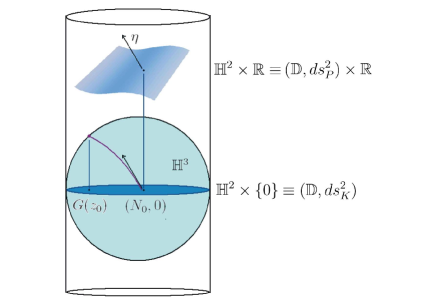
Figura 1: The hyperbolic Gauss map for surfaces in $\mathbb{H}^{2}\times\mathbb{R}$.

The result of this is a map $G:\Sigma\to(\mathbb{D},ds_{K}^{2})\equiv\mathbb{H}^{2}$ which is the hyperbolic Gauss map of $\psi$. Its most remarkable property is that it is harmonic for $H=1/2$ surfaces, as we explain next.

CMC one half surfaces in $\mathbb{H}^{2}\times\mathbb{R}$

The existence of the canonical examples of minimal surfaces in ${\rm{Nil}_{3}}$ will be shown in terms of their sister surfaces in $\mathbb{H}^{2}\times\mathbb{R}$, so let us first recall some facts about surfaces with $H=1/2$ in $\mathbb{H}^{2}\times\mathbb{R}$.

To start, let $G:\Sigma\to\mathbb{H}^{2}$ denote a harmonic map from the Riemann surface $\Sigma$ into $\mathbb{H}^{2}$. Then the quadratic differential $\langle{G_{z}},{G_{z}}\rangle dz^{2}$ is holomorphic on $\Sigma$, and it is called the Hopf differential of the harmonic map $G$. Following [FeMi1], we say that a harmonic map admits Weierstrass data $\{Q,\tau_{0}\}$ if there exists $\tau_{0}:\Sigma\rightarrow(0,\infty)$ a smooth positive function such that

$$\langle{dG},{dG}\rangle=Qdz^{2}+\left(\frac{\tau_{0}}{4}+\frac{4|Q|^{2}}{\tau_{0}}\right)|dz|^{2}+\bar{Q}d\bar{z}^{2}\mathchar 46\relax$$

The connection between $H=1/2$ surfaces in $\mathbb{H}^{2}\times\mathbb{R}$ and harmonic maps into $\mathbb{H}^{2}$ was studied in [FeMi1]. We condense the most relevant features of this connection in the following result.

Convention: from now on, a surface in $\mathbb{H}^{2}\times\mathbb{R}$ with r.v.p. will always be assumed to be canonically oriented, meaning this that its unit normal is upwards pointing.

Theorem 5 ([FeMi1])

The hyperbolic Gauss map $G:\Sigma\rightarrow\mathbb{H}^{2}$ of a $H=1/2$ surface $\psi:\Sigma\rightarrow\mathbb{H}^{2}\times\mathbb{R}$ with regular vertical projection is harmonic. Moreover, if $-Qdz^{2}$ denotes the Abresch-Rosenberg differential of the surface, $\lambda|dz|^{2}$ its metric and $u$ its angle function, then the quantities $\{Q,\lambda u^{2}\}$ are Weierstrass data for $G$. In particular the Hopf differential of $G$ is $Qdz^{2}$.

Conversely, let $\Sigma$ be a simply-connected Riemann surface and $G:\Sigma\to\mathbb{H}^{2}$ be a harmonic map admitting Weierstrass data $\{Q,\tau_{0}\}$.Then

1. If $G$ is singular on an open subset of $\Sigma$ then it parametrizes a piece of a geodesic in $\mathbb{H}^{2}$. Moreover, there exists a $1$-parameter family of $H=1/2$ graphs in $\mathbb{H}^{2}\times\mathbb{R}$, invariant under a $1$-parameter subgroup of isometries, such that $G$ is the hyperbolic Gauss map of any of them. These surfaces are described in [Sa] (see also [FeMi1, Dan2]), and they are open pieces of the sister surfaces of the saddle-type minimal graphs in ${\rm{Nil}_{3}}$.

2. If not, let $z_{0}\in\Sigma$ be a regular point of $G$. Then for any $\vartheta_{0}\in\mathbb{C}$ there exists a unique $H=1/2$ surface $\psi=(N,h):\Sigma\to\mathbb{H}^{2}\times\mathbb{R}$ with r.v.p., having $G$ as its hyperbolic Gauss map and satisfying:

   1. $\tau_{0}=\lambda u^{2}$, where $\lambda$ is the conformal factor of the metric of $\psi$ and $u$ its angle function,

   2. $h_{z}(z_{0})=\vartheta_{0}$.

   Moreover,

   $$N=\frac{8\mathop{\rm Re}\nolimits\Big{(}G_{z}\big{(}\tau_{0}h_{\bar{z}}-4\overline{Q}h_{z}\big{)}\Big{)}}{\tau_{0}^{2}-16|Q|^{2}}+G\,\sqrt{\displaystyle\frac{\tau_{0}+4|h_{z}|^{2}}{\tau_{0}}},$$

   and $h:\Sigma\rightarrow\mathbb{R}$ is the unique (up to additive constants) solution to the differential system below such that $h_{z}(z_{0})=\vartheta_{0}$:

   $$\left\{\begin{array}[]{lll}h_{zz}&=&(\log\tau_{0})_{z}\,h_{z}-Q\,\sqrt{\displaystyle\frac{\tau_{0}+4|h_{z}|^{2}}{\tau_{0}}},\\ \\ h_{z\bar{z}}&=&\displaystyle\frac{1}{4}\sqrt{\tau_{0}(\tau_{0}+4|h_{z}|^{2})}\mathchar 46\relax\end{array}\right\mathchar 46\relax$$ (2.4)

Remark 6

A straightforward consequence of the definition of the hyperbolic Gauss map is that if two surfaces in $\mathbb{H}^{2}\times\mathbb{R}$ with r.v.p. are congruent by an isometry preserving the orientation of the fibers, then their respective hyperbolic Gauss maps differ by an isometry of $\mathbb{H}^{2}$. As a result, if two harmonic maps $G_{1},G_{2}$ into $\mathbb{H}^{2}$ differ by an isometry, then the two families of $H=1/2$ surfaces obtained from $G_{1}$ and $G_{2}$ via Theorem 5 just differ by an isometry of $\mathbb{H}^{2}\times\mathbb{R}$ preserving the orientation of the fibers. This is a consequence of the uniqueness part of Theorem 5.

The canonical examples in ${\rm{Nil}_{3}}$

In what follows, $\Sigma$ will denote a simply-connected open Riemann surface, that will be assumed without loss of generality to be $\Sigma=\mathbb{C}$ or $\Sigma=\mathbb{D}$.

In [FeMi1] we proved the existence of a large family of complete minimal surfaces in ${\rm{Nil}_{3}}$ that are local vertical graphs. More specifically, we showed:

Theorem 7 ([FeMi1])

Let $Qdz^{2}$ denote a holomorphic quadratic differential on $\Sigma$, which is non-zero if $\Sigma=\mathbb{C}$. Then there exists (at least) a complete minimal surface with regular vertical projection in ${\rm{Nil}_{3}}$ whose Abresch-Rosenberg differential is $Qdz^{2}$.

It is relevant for our purposes to explain how these examples are constructed. Let $Qdz^{2}$ be a holomorphic quadratic differential as above. By [Wan, WaAu] there exists a complete spacelike CMC $1/2$ surface $f:\Sigma\to\mathbb{L}^{3}$ in the Lorentz-Minkowski $3$-space $\mathbb{L}^{3}$ whose Hopf differential is $Qdz^{2}$. Here, recall that $\mathbb{L}^{3}$ is just $\mathbb{R}^{3}$ endowed with the Lorentzian metric $\langle,\rangle=dx_{1}^{2}+dx_{2}^{2}-dx_{3}^{2}$ in canonical coordinates, and that an immersed surface $f:\Sigma\rightarrow\mathbb{L}^{3}$ is called spacelike if its induced metric $\langle df,df\rangle$ is Riemannian.

Let $\nu:\Sigma\rightarrow\mathbb{H}^{2}\cup\mathbb{H}_{-}^{2}\subset\mathbb{L}^{3}$ denote its Gauss map, which is well known to be harmonic. Now let $G:\Sigma\rightarrow\mathbb{H}^{2}$ denote the harmonic map given by $G=\nu$ if $\nu$ is future-pointing, or by the vertical symmetry of $\nu$ in $\mathbb{L}^{3}$ otherwise. Thus, if $\langle df,df\rangle=\tau_{0}|dz|^{2}$ denotes the induced metric of $f$, it turns out (see [FeMi1]) that $\{Q,\tau_{0}\}$ are Weierstrass data for $G$. Then the $H=1/2$ surfaces in $\mathbb{H}^{2}\times\mathbb{R}$ constructed from $G$ and $\tau_{0}$ via Theorem 5 are complete (since $\tau_{0}|dz|^{2}=\lambda u^{2}|dz|^{2}$ is complete), have regular vertical projection, and Abresch-Rosenberg differential $-Qdz^{2}$. Consequently, the sister surfaces of these examples are complete minimal surfaces in ${\rm{Nil}_{3}}$ with regular vertical projection and whose Abresch-Rosenberg differential is $Qdz^{2}$.

Let us mention that $f:\Sigma\rightarrow\mathbb{L}^{3}$ is unique, in the sense that if $\widetilde{f}:\Sigma\rightarrow\mathbb{L}^{3}$ is another complete spacelike $H=1/2$ surface with Hopf differential $Qdz^{2}$, then $\widetilde{f}=\Phi\circ f$ for some positive rigid motion $\Phi$ of $\mathbb{L}^{3}$. Thereby, if we start with some $\widetilde{f}$ different from (but congruent to) $f$, the harmonic map $\widetilde{G}:\Sigma\rightarrow\mathbb{H}^{2}$ we obtain following the process above differs from $G$ at most by an isometry of $\mathbb{H}^{2}$.

Thus, bearing in mind Remark 6 we conclude that the families of $H=1/2$ surfaces in $\mathbb{H}^{2}\times\mathbb{R}$ obtained, respectively, from $f$ and $\widetilde{f}$, differ at most by an isometry of $\mathbb{H}^{2}\times\mathbb{R}$ that preserves the orientation of the fibers. This means by the sister correspondence that no new examples in ${\rm{Nil}_{3}}$ appear if in the above process we consider $\Phi\circ f$ instead of $f$ for any positive rigid motion $\Phi$ of $\mathbb{L}^{3}$.

Finally, let us comment some properties of these minimal examples in ${\rm{Nil}_{3}}$, that one should keep in mind for what follows.

• By Theorem 5 and the uniqueness property we have just pointed out, the above procedure yields in the generic case (i.e. in the case where the Gauss map $G$ does not have a $1$-parameter symmetry group) a $2$-parameter family of non-congruent complete minimal surfaces in ${\rm{Nil}_{3}}$ with the same Abresch-Rosenberg differential. These two continuous parameters come from the variation of the initial condition $h_{z}(z_{0})=\vartheta_{0}$. Although the elements of this family are non-congruent in general (e.g. if the Gauss map has no symmetries), it happens that for minimal surfaces in ${\rm{Nil}_{3}}$ invariant under a $1$-parameter subgroup of isometries many of the elements of the $2$-parameter family are congruent to each other. A detailed discussion on this topic can be found in page 1165 of [FeMi1] (see also [Dan2]).

• The only minimal surfaces in ${\rm{Nil}_{3}}$ with $Q=0$ and $\Sigma=\mathbb{C}$ are vertical planes, which do not have regular vertical projection. Besides, minimal surfaces with $Q=0$ and $\Sigma=\mathbb{D}$ are the horizontal minimal umbrellas [AbRo2, Dan1].

• When $\Sigma=\mathbb{C}$ and $Qdz^{2}=c\,dz^{2}$, $c\in\mathbb{C}\setminus\{0\}$ the spacelike surface $f:\Sigma\to\mathbb{L}^{3}$ defined above is the hyperbolic cylinder, whose Gauss map parametrizes a piece of a geodesic in $\mathbb{H}^{2}$. This corresponds to Case 1 in Theorem 5, and therefore, the corresponding family of canonical examples is the $1$-parameter family of saddle type surfaces, as stated in the introduction.

• Any of the minimal surfaces in ${\rm{Nil}_{3}}$ given by Theorem 7 verifies that $u^{2}\,g$ is a complete Riemannian metric, where here $g$ and $u$ stand, respectively, for the induced metric and the angle function of the minimal surface.

Definition 8 (Canonical Examples)

A minimal surface $X:\Sigma\to{\rm{Nil}_{3}}$ will be called a canonical example if it is one of the complete minimal surfaces with regular vertical projection given by Theorem 7.

We will show in the next section that the canonical examples in ${\rm{Nil}_{3}}$ are exactly the entire minimal graphs in ${\rm{Nil}_{3}}$. This justifies the terminology we have used.

3 Solution to the Bernstein problem in ${\rm{Nil}_{3}}$

This section is devoted to the proof of Theorem 1. First of all, we prove that any canonical example is an entire graph. This will be obtained as a consequence of the following Lemma.

Lemma 9

Let $X:\Sigma\to\mathbb{E}^{3}(\kappa,\tau)$ be a surface in the homogeneous $3$-manifold $\mathbb{E}^{3}(\kappa,\tau)$. Denote by $F:\Sigma\to\mathcal{M}^{2}(\kappa)$ its vertical projection and by $g_{F}$ the induced metric of $F$ in $\Sigma$. Then, for every $v\in\mathfrak{X}(\Sigma)$,

$$u^{2}\,g(v,v)\leq g_{F}(v,v)\leq g(v,v),$$ (3.1)

where $g$ denotes the induced metric of the immersion $X$ and $u$ is the angle function.

• Let $z$ be a conformal parameter for $X$ so that the induced metric on $\Sigma$ is written as $g=\lambda|dz|^{2}$. Keeping the notation introduced in Section 2 we have by (2.1) that the metric of the vertical projection is written with respect to $z$ as

  $$g_{F}=-A^{2}dz^{2}+(\lambda-2|A|^{2})|dz|^{2}-\bar{A}^{2}d\bar{z}^{2}\mathchar 46\relax$$ (3.2)

  Then the eigenvalues $\rho_{1}\geq\rho_{2}$ of the symmetric bilinear form $g_{F}$ with respect to the flat metric $|dz|^{2}$ are the solutions of the equation $\mathop{\rm det}\nolimits[g_{F}-\rho\,\mbox{Id}]=0$, which by (C.4) yields

  $$\rho_{1}=\lambda,\hskip 28.45274pt\rho_{2}=\lambda-4|A|^{2}=\lambda u^{2}\mathchar 46\relax$$

  From this we obtain (3.1) immediately.

  $\Box$

From this Lemma we can now prove that canonical examples are entire minimal graphs. Indeed, if $X:\Sigma\to{\rm{Nil}_{3}}$ is a canonical example with angle function $u$ and induced metric $g$ on $\Sigma$, the metric $u^{2}\,g$ is complete, and thus Lemma 9 gives the completeness of $g_{F}$. As a consequence, $F:(\Sigma,g_{F})\rightarrow\mathbb{R}^{2}$ is a local isometry with $(\Sigma,g_{F})$ complete. In these conditions, $F$ must necessarily be a (surjective) covering map. Hence, the vertical projection $F:\Sigma\to\mathbb{R}^{2}$ is a global diffeomorphism and $X$ is an entire graph.

This fact together with the comments in Section 2 regarding the canonical examples in ${\rm{Nil}_{3}}$ proves the existence part of Theorem 1.

Once here, in order to end up the proof of Theorem 1, it remains only to check that any entire minimal graph in ${\rm{Nil}_{3}}$ is one of the canonical examples. For that, let us first provide a geometric interpretation of the differential system (2.4).

From now on, $\Sigma$ will denote an open simply connected Riemann surface.

Let $f:\Sigma\rightarrow\mathbb{L}^{3}$ denote a spacelike surface with future-pointing Gauss map, with induced metric $\tau_{0}|dz|^{2}$ and Hopf differential $Qdz^{2}$. Then:

1. If $H=1/2$, its Gauss map $G:\Sigma\rightarrow\mathbb{H}^{2}$ is harmonic and admits the Weierstrass data $\{Q,\tau_{0}\}$. In addition, $Q,\tau_{0}$ verify the Gauss-Codazzi equations in $\mathbb{L}^{3}$ for $H=1/2$, i.e.

   $$(\log\tau_{0})_{z\bar{z}}=\frac{\tau_{0}}{8}-\frac{2|Q|^{2}}{\tau_{0}},\hskip 34.14322ptQ_{\bar{z}}=0\mathchar 46\relax$$ (3.3)

2. Conversely, if a harmonic map $G:\Sigma\rightarrow\mathbb{H}^{2}$ admits Weierstrass data $\{Q,\tau_{0}\}$, then by [FeMi1, Lemma 4] the pair $Q,\tau_{0}$ satisfy (3.3). Therefore there exists some (unique up to positive isometries) spacelike $H=1/2$ surface $f:\Sigma\rightarrow\mathbb{L}^{3}$ with metric $\tau_{0}|dz|^{2}$ and Hopf differential $Qdz^{2}$.

Bearing these facts in mind, we have

Lemma 10

Let $\{Q,\tau_{0}\}$ be Weierstrass data of a harmonic map $G:\Sigma\rightarrow\mathbb{H}^{2}$, and let $f:\Sigma\rightarrow\mathbb{L}^{3}$ denote an arbitrary spacelike $H=1/2$ surface in $\mathbb{L}^{3}$ with Hopf differential $-Qdz^{2}$ and metric $\tau_{0}|dz|^{2}$ (which is unique up to positive isometries of $\mathbb{L}^{3}$).

Then a function $h:\Sigma\rightarrow\mathbb{R}$ is a solution to (2.4) if and only if $h=-\langle f,a\rangle$, where $a\in\mathbb{L}^{3}$ verifies $\langle a,a\rangle=-1$ and belongs to the connected component of the two-sheeted hyperboloid $\mathbb{H}^{2}\cup\mathbb{H}_{-}^{2}\subset\mathbb{L}^{3}$ where the Gauss map of $f$ lies.

• Let us first of all prove that $h:=-\langle f,a\rangle$ as above solves (2.4). For that, we first rewrite (2.4) as

  $$\left\{\begin{array}[]{lll}h_{zz}&=&(\log\tau_{0})_{z}\,h_{z}-\displaystyle\frac{4Q}{\tau_{0}}h_{z\bar{z}},\\ \\ h_{z\bar{z}}&=&\displaystyle\frac{1}{4}\sqrt{\tau_{0}(\tau_{0}+4|h_{z}|^{2})}\mathchar 46\relax\end{array}\right\mathchar 46\relax$$ (3.4)

  On the other hand, by the structure equations for $f$ in $\mathbb{L}^{3}$ we have

  $$f_{zz}=(\log\tau_{0})_{z}f_{z}-QG_{f},\hskip 28.45274ptf_{z\bar{z}}=\frac{\tau_{0}}{4}G_{f},$$ (3.5)

  where $G_{f}:\Sigma\rightarrow\mathbb{H}^{2}\cup\mathbb{H}_{-}^{2}$ is the Gauss map of $f$. So, it is clear by (3.5) that $h=-\langle f,a\rangle$ verifies the first equation in (3.4) for every $a\in\mathbb{L}^{3}$. To see that $h$ also verifies the second one we first observe that, by (3.5),

  $$h_{z\bar{z}}=-\frac{\tau_{0}}{4}\langle a,G_{f}\rangle\mathchar 46\relax$$ (3.6)

  Besides,

  $$a=\frac{2\langle a,f_{\bar{z}}\rangle}{\tau_{0}}\,f_{z}+\frac{2\langle a,f_{z}\rangle}{\tau_{0}}\,f_{\bar{z}}-\langle a,G_{f}\rangle G_{f},$$

  so from $\langle a,a\rangle=-1$ we obtain

  $$\langle a,G_{f}\rangle^{2}=1+\frac{4|\langle a,f_{z}\rangle|^{2}}{\tau_{0}}\mathchar 46\relax$$ (3.7)

  Putting together (3.6), (3.7) and taking into account that $\langle a,G_{f}\rangle<0$ by hypothesis, we conclude that

  $$h_{z\bar{z}}=\frac{\tau_{0}}{4}\sqrt{1+\frac{4|\langle a,f_{z}\rangle|^{2}}{\tau_{0}}}=\displaystyle\frac{1}{4}\sqrt{\tau_{0}(\tau_{0}+4|h_{z}|^{2})},$$

  i.e. $h$ satisfies also the second equation of (3.4), and therefore (2.4) as claimed.

  Finally, in order to see that all the solutions of (2.4) are of this form, we will see that for every $\vartheta_{0}\in\mathbb{C}$ there is some $a\in\mathbb{H}^{2}\cup\mathbb{H}_{-}^{2}$ in the connected component of $G(\Sigma)$ such that

  $$-\langle f_{z}(z_{0}),a\rangle=\vartheta_{0}$$ (3.8)

  for a fixed point $z_{0}\in\Sigma$. Once this is done, the result will follow by the uniqueness (up to additive constants) of solutions to (2.4) with the initial condition $h_{z}(z_{0})=\vartheta_{0}$.

  To prove this claim, observe first that (3.8) is a linear system of two equations for $a=(a_{1},a_{2},a_{3})$. So, as $df$ is spacelike and regular, the solution to the system above is an affine timelike line in $\mathbb{L}^{3}$. This line meets both $\mathbb{H}^{2}$ and $\mathbb{H}_{-}^{2}$, what ensures the existence of some $a$ with $\langle a,a\rangle=-1$ in the connected component of $G(\Sigma)$ that fulfills the initial condition (3.8).

$\Box$

The next Lemma is the key ingredient to prove this classification result. We also think that this result has importance by itself beyond the use that we give it here. In particular, it may allow to construct a Sym-Bobenko type formula for $H=1/2$ surfaces in $\mathbb{H}^{2}\times\mathbb{R}$ and for minimal surfaces in ${\rm{Nil}_{3}}$.

Lemma 11

Let $\psi=(N,h):\Sigma\to\mathbb{H}^{2}\times\mathbb{R}$ be a $H=1/2$ surface with regular vertical projection, and let $-Qdz^{2}$ denote its Abresch-Rosenberg differential. Let $X=(F,t):\Sigma\to{\rm{Nil}_{3}}$ be any of its sister minimal surfaces in ${\rm{Nil}_{3}}$.

Then there is some $\varepsilon=\pm 1$ such that $f:=(F,\varepsilon h):\Sigma\to\mathbb{L}^{3}$ is the unique (up to positive isometries) spacelike surface with $H=1/2$ in $\mathbb{L}^{3}$ with induced metric $u^{2}g$ and Hopf differential $-Qdz^{2}$. Here $g,u$ are, respectively, the metric and the angle function of $X$ (and of $\psi$).

• Let $z$ denote a conformal parameter on $\Sigma$, and write $g=\lambda|dz|^{2}$ for the common induced metric of both $\psi$ and $X$. Let us point out that $Qdz^{2}$ is the Hopf differential of the (harmonic) hyperbolic Gauss map $G:\Sigma\rightarrow\mathbb{H}^{2}$ of $\psi$, and that $G$ admits the Weierstrass data $\{Q,\tau_{0}:=\lambda u^{2}\}$. Thus $\{-Q,\tau_{0}\}$ verify the Gauss-Codazzi equations (3.3), and there exists a unique (up to positive isometries of $\mathbb{L}^{3}$) spacelike $H=1/2$ immersion $f_{0}:\Sigma\rightarrow\mathbb{L}^{3}$ with induced metric $\tau_{0}|dz|^{2}$ and Hopf differential $-Qdz^{2}$.

  Let us denote $f_{0}=(P,r):\Sigma\rightarrow\mathbb{L}^{3}$. Then by Lemma 10 any solution to (2.4) is of the form $-\langle f_{0},a\rangle$ for some $a\in\mathbb{H}^{2}\cup\mathbb{H}_{-}^{2}$. In particular, the height function $h$ of $\psi=(N,h)$ is of this form, by Theorem 5. Thus, by composing with an adequate positive isometry of $\mathbb{L}^{3}$ if necessary, we may assume that $h=r$.

  With this, the metric of the projection $P$ is

  $$\langle dP,dP\rangle=h_{z}^{2}dz^{2}+\left(\tau_{0}+2|h_{z}|^{2}\right)|dz|^{2}+h_{\bar{z}}^{2}d\bar{z}^{2}\mathchar 46\relax$$

  On the other hand, let $X=(F,t)$ be an arbitrary sister minimal surface in ${\rm{Nil}_{3}}$ of $\psi=(N,h)$. Then, by (2.2) and (2.3) we have that $A=ih_{z}$, where $A$ belongs to the fundamental data of $X$. Now, using this together with (3.2) and formula (C.4) we infer that

  $$\begin{array}[]{lll}\langle dF,dF\rangle&=&-A^{2}dz^{2}+(\lambda-2|A|^{2})|dz|^{2}-\bar{A}^{2}d\bar{z}^{2}\\ &=&h_{z}^{2}dz^{2}+(\lambda u^{2}+2|h_{z}|^{2})|dz|^{2}+h_{\bar{z}}^{2}d\bar{z}^{2}\\ &=&h_{z}^{2}dz^{2}+\left(\tau_{0}+2|h_{z}|^{2}\right)|dz|^{2}+h_{\bar{z}}^{2}d\bar{z}^{2},\end{array}$$

  i.e. $\langle dF,dF\rangle=\langle dP,dP\rangle$. Then $F=\Phi\circ P$ for some isometry $\Phi:\mathbb{R}^{2}\rightarrow\mathbb{R}^{2}$. Now, this isometry can be extended to a positive rigid motion $\Psi$ of $\mathbb{L}^{3}$, which may possibly reverse time-orientation. So, we can conclude the existence of some $\varepsilon=\pm 1$ such that $\Psi\circ f_{0}=(F,\varepsilon h)=:f$. This concludes the proof of Lemma 11.

  $\Box$

Once here we can finish the proof of Theorem 1. For that, let us consider $X=(F,t):\Sigma\to{\rm{Nil}_{3}}$ to be an entire minimal graph with Abresch-Rosenberg differential $Qdz^{2}$. First, take its sister $H=1/2$ immersion $\psi=(N,h):\Sigma\rightarrow\mathbb{H}^{2}\times\mathbb{R}$, which has Abresch-Rosenberg differential $-Qdz^{2}$, induced metric $\lambda|dz|^{2}$, angle function $u$ (we shall assume that $u>0$ without loss of generality), and is defined up to isometries of $\mathbb{H}^{2}\times\mathbb{R}$ preserving the orientations of both base and fibers. Let $G:\Sigma\rightarrow\mathbb{H}^{2}$ denote the (harmonic) hyperbolic Gauss map of one of such sister immersions $\psi$. Then $X:\Sigma\rightarrow{\rm{Nil}_{3}}$ will be a canonical example if $G$ differs at most by a rigid motion of $\mathbb{L}^{3}$ from the Gauss map $\nu:\Sigma\rightarrow\mathbb{H}^{2}\cup\mathbb{H}_{-}^{2}\subset\mathbb{L}^{3}$ of some complete spacelike surface $f_{0}:\Sigma\rightarrow\mathbb{L}^{3}$ with $H=1/2$. This is just a consequence of the proper construction of the canonical examples.

But now, by Theorem 5, the hyperbolic Gauss map $G$ admits the Weierstrass data $\{Q,\lambda u^{2}\}$. This means that there is a unique (up to positive rigid motions) spacelike surface $f_{0}:\Sigma\rightarrow\mathbb{L}^{3}$ with $H=1/2$, induced metric $\lambda u^{2}|dz|^{2}$ and Hopf differential $Qdz^{2}$. By composing if necessary with a positive isometry of $\mathbb{L}^{3}$ that reverses time-orientation we can assume that the Gauss map of $f_{0}$ is future-pointing. Moreover, it has the Weierstrass data $\{Q,\lambda u^{2}\}$. Now by [FeMi1, Lemma 6] this Gauss map differs from $G$ at most by a rigid motion.

So, we only need to check that $f_{0}$ is complete, i.e that $\lambda u^{2}|dz|^{2}$ is complete for $X=(F,t):\Sigma\rightarrow{\rm{Nil}_{3}}$. By Lemma 11 we know the existence of some spacelike $H=1/2$ surface $f=(P,r):\Sigma\rightarrow\mathbb{L}^{3}$ such that $P=F$. Thus, $f$ is an entire spacelike graph in $\mathbb{L}^{3}$. Now, a result in [ChYa] establishes that all spacelike entire CMC graphs in $\mathbb{L}^{3}$ have complete induced metric (here the CMC assumption is essential). In particular $f$ is complete. But again by Lemma 11, the induced metric of $f$ is $\lambda u^{2}|dz|^{2}$. Thus, this metric is complete and $X$ must be a canonical example.

We have then proved:

Theorem 12

A minimal surface in ${\rm{Nil}_{3}}$ is an entire vertical graph if and only if it is a canonical example.

From this result and the description of the canonical examples in Section 2 we obtain Theorem 1. Moreover, as a byproduct of our proof we get the following characterization of the entire minimal graphs in ${\rm{Nil}_{3}}$.

Corollary 13

Let $X$ be a minimal surface in ${\rm{Nil}_{3}}$ with metric $g$ and angle function $u$. Then $X$ is an entire graph if and only if $u^{2}\,g$ is a complete Riemannian metric.

Observe that if $u^{2}g$ is a complete metric for an arbitrary surface in any homogeneous space $\mathbb{E}^{3}(\kappa,\tau)$ (not necessarily with CMC), then the surface must be an entire graph by Lemma 9. However, the converse is not true in general. For instance, the entire graph

$$x_{3}(x_{1},x_{2})=x_{2}\,e^{1/(1-x_{1}^{2}-x_{2}^{2})},\hskip 28.45274ptx_{1}^{2}+x_{2}^{2}<1,$$

in $\mathbb{H}^{2}\times\mathbb{R}\equiv(\mathbb{D},ds_{P}^{2})\times\mathbb{R}$, has non-complete $u^{2}g$ metric. Indeed, it is an elementary computation to check that the divergent curve $\alpha(t):=(t,0,x_{3}(t,0))$, $0\leq t<1$, lies on the graph and has finite $u^{2}g$ length.

4 Surfaces with $H=1/2$ in $\mathbb{H}^{2}\times\mathbb{R}$ and further results

In view of the results of the present paper and Daniel’s Lawson-type correspondence, it is a natural problem to ask for the classification of the entire vertical graphs with $H=1/2$ in the product space $\mathbb{H}^{2}\times\mathbb{R}$ (see [FeMi1, Sa]). The following result, which constitutes an improvement of [FeMi1, Theorem 16], shows that the class of solutions to such Bernstein-type problem in $\mathbb{H}^{2}\times\mathbb{R}$ is at least as large as the class of entire minimal graphs in ${\rm{Nil}_{3}}$.

Proposition 14

The sister surface of an entire minimal graph in ${\rm{Nil}_{3}}$ is an entire $H=1/2$ graph in $\mathbb{H}^{2}\times\mathbb{R}$.

Consequently, given a holomorphic quadratic differential $Qdz^{2}$ on $\Sigma\equiv\mathbb{C}$ or $\mathbb{D}$ which is not identically zero if $\Sigma\equiv\mathbb{C}$, there exists a $2$-parametric family of (generically non-congruent) entire $H=1/2$ graphs in $\mathbb{H}^{2}\times\mathbb{R}$ whose Abresch-Rosenberg differential is $Qdz^{2}$.

• It follows directly from Corollary 13, Lemma 9 and the fact that the metric $\lambda u^{2}|dz|^{2}$ is invariant by the sister correspondence.

  $\Box$

Remark 15

By Corollary 13, the entire $H=1/2$ graphs in Proposition 14 are characterized by the fact that $u^{2}g$ is a complete metric. It is natural to ask if these are the only entire $H=1/2$ graphs in $\mathbb{H}^{2}\times\mathbb{R}$. Unfortunately, we cannot proceed in this setting as we did for minimal graphs in ${\rm{Nil}_{3}}$, since we do not have a good control on the vertical projection for $H=1/2$ surfaces in $\mathbb{H}^{2}\times\mathbb{R}$. Let us also point out that the existence of an entire $H=1/2$ graph in $\mathbb{H}^{2}\times\mathbb{R}$ for which $u^{2}g$ is not complete remains unknown.

Another interesting application of the arguments used in the proof of Theorem 1 is the following.

Corollary 16

Let $\psi:\Sigma\rightarrow\mathbb{H}^{2}\times\mathbb{R}$ denote a $H=1/2$ surface with regular vertical projection such that its hyperbolic Gauss map $G:\Sigma\rightarrow\mathbb{H}^{2}$ is a global diffeomorphism. Assume additionally that its Abresch-Rosenberg differential vanishes somewhere. Then $\psi$ is one of the entire graphs given in Proposition 14.

• By Theorem 5, $G$ has Weierstrass data $\{-Q,\lambda u^{2}\}$, where $Qdz^{2}$ is the Abresch-Rosenberg differential of $\psi$. Thus

  $$\langle dG,dG\rangle=-Qdz^{2}+\left(\frac{\lambda u^{2}}{4}+\frac{4|Q|^{2}}{\lambda u^{2}}\right)|dz|^{2}-\bar{Q}d\bar{z}^{2}\mathchar 46\relax$$

  If we now compute the eigenvalues $\rho_{1}\geq\rho_{2}$ of $\langle dG,dG\rangle$ with respect to the flat metric $|dz|^{2}$, we obtain

  $$\rho_{1}=\frac{\lambda u^{2}}{4}(1+d_{G})^{2},\hskip 28.45274pt\rho_{2}=\frac{\lambda u^{2}}{4}(1-d_{G})^{2},\hskip 14.22636ptd_{G}:=\frac{4|Q|}{\lambda u^{2}}\mathchar 46\relax$$

  Hence, as $\langle dG,dG\rangle$ is complete by hypothesis, the metric $\rho_{1}|dz|^{2}$ is complete. But since $\langle dG,dG\rangle$ is regular, we infer that $4|Q|\neq\lambda u^{2}$ at every point. So, as $Q$ vanishes somewhere we get $d_{G}\in[0,1)$. By this fact and the completeness of $\rho_{1}|dz|^{2}$ we conclude that $\lambda u^{2}|dz|^{2}$ is a complete metric, and hence by Corollary 13 that $\psi$ is one of the entire graphs of Proposition 14.

  $\Box$

Remark 17

If $G:\Sigma\rightarrow\mathbb{H}^{2}$ admits Weierstrass data $\{Q,\tau_{0}\}$ such that $Q$ never vanishes, then there is a second set of Weierstrass data $\{Q,\tau^{\sharp}:=16|Q|^{2}/\tau_{0}\}$ available for $G$. These two sets of data give rise to parallel-like $H=1/2$ surfaces $\psi,\psi^{\sharp}$ in $\mathbb{H}^{2}\times\mathbb{R}$ with the same hyperbolic Gauss map $G$ (see [FeMi1, Theorem 19]). In these conditions, we can still say that if $G$ is a global diffeomorphism, then one of $\psi,\psi^{\sharp}$ is an entire graph of Proposition 14. This follows by a simple modification of the last part of the above proof.

Remark 18

The existence of harmonic diffeomorphisms from $\mathbb{C}$ onto $\mathbb{H}^{2}$ has been recently proved by Collin and Rosenberg in [CoRo].

It is interesting to observe that Corollary 16 has a counterpart for minimal surfaces in ${\rm{Nil}_{3}}$. Indeed, in [Dan2] Daniel gave an extension to the case of minimal surfaces in ${\rm{Nil}_{3}}$ of the harmonicity theory for the hyperbolic Gauss map of $H=1/2$ surfaces in $\mathbb{H}^{2}\times\mathbb{R}$. In this ${\rm{Nil}_{3}}$ setting, the harmonic Gauss map is simply the usual Gauss map of a surface with regular vertical projection (taking values on the upper hemisphere of the Lie algebra of ${\rm{Nil}_{3}}$), composed with stereographic projection. This gives a Gauss map $g:\Sigma\rightarrow\mathbb{D}$ which is harmonic for minimal surfaces when we endow $\mathbb{D}$ with the Poincaré metric. See [Dan2] for more details.

Taking these facts into consideration, one can see that the proof of Corollary 16 also works in ${\rm{Nil}_{3}}$, and so we obtain:

Corollary 19

Let $X:\Sigma\rightarrow{\rm{Nil}_{3}}$ denote a minimal surface with regular vertical projection, and whose Abresch-Rosenberg differential vanishes somewhere. Assume that its usual Gauss map is a global diffeomorphism onto the upper hemisphere $\mathbb{S}_{+}^{2}$. Then $X$ is canonical example.

We end up with two closing remarks regarding our results. The study of the Bernstein problem in ${\rm{Nil}_{3}}$ presented here makes constant use of the theory of $H=1/2$ surfaces in $\mathbb{H}^{2}\times\mathbb{R}$, for instance, for the construction of the canonical examples. It is nonetheless very likely that our arguments can be modified in certain aspects to give an alternative proof of Theorem 1 without using $\mathbb{H}^{2}\times\mathbb{R}$ at all. This possibility is given by the harmonicity of the Gauss map for minimal surfaces in ${\rm{Nil}_{3}}$ [Dan2]. We have followed here the path across $\mathbb{H}^{2}\times\mathbb{R}$ to give a natural continuation of the work [FeMi1], which is where the canonical examples were first constructed, and also because we believe that this more flexible perspective may give a clearer global picture of CMC surface theory in homogeneous $3$-manifolds. Lemma 11 is an example of the benefits that this perspective can have.

Let us finally point out that there are still relevant problems regarding the global geometry of entire minimal graphs in ${\rm{Nil}_{3}}$. For instance, the problem of describing the global behavior of canonical examples in ${\rm{Nil}_{3}}$ is specially interesting. Another interesting inquiry line is to give concrete geometric conditions that characterize the horizontal umbrellas or the saddle-type minimal graphs among all canonical examples (let us point out that these minimal surfaces are the only examples invariant by a $1$-parameter isometry subgroup).

Added after revision

Very recently, L. Hauswirth, H. Rosenberg and J. Spruck [HRS] have proved that any complete local graph with mean curvature one half in $\mathbb{H}^{2}\times\mathbb{R}$ must be an entire graph. After that work, the analogous result for minimal surfaces in ${\rm{Nil}_{3}}$ has been proved by B. Daniel and L. Hauswirth [DaHa].

As a consequence, it was obtained in [DaHa] that any entire graph with $H=1/2$ in $\mathbb{H}^{2}\times\mathbb{R}$ must be the sister surface of a canonical example in ${\rm{Nil}_{3}}$. This result gives a classification of the entire $H=1/2$ graphs in $\mathbb{H}^{2}\times\mathbb{R}$, proving that any such entire graph is one of the examples given in Proposition 14.

References

- [AbRo1] U. Abresch, H. Rosenberg, A Hopf differential for constant mean curvature surfaces in and , Acta Math. 193 (2004), 141–174.
- [AbRo2] U. Abresch, H. Rosenberg, Generalized Hopf differentials, Mat. Contemp. 28 (2005), 1–28.
- [ADR] L.J. Alías, M. Dajczer, H. Rosenberg, The Dirichlet problem for CMC surfaces in Heisenberg space, Calc. Var. Partial Diff. Equations, 30 (2007), 513–522.
- [BSV] V. Barone-Adesi, F. Serra-Cassano, D. Vittone, The Bernstein problem for intrinsic graphs in the Heisenberg group and calibrations, Calc. Var. Partial Diff. Equations, 30 (2007), 17–49.
- [Bry] R.L. Bryant, Surfaces of mean curvature one in hyperbolic space, Astérisque, 154-155 (1987), 321–347.
- [ChYa] S.Y. Cheng, S.T. Yau, Maximal spacelike hypersurfaces in the Lorentz-Minkowski spaces, Ann. of Math. 104 (1976), 407–419.
- [CHMY] J.H. Cheng, J.F Hwang, A. Malchiodi, P. Yang, Minimal surfaces in pseudohermitian geometry, Ann. Sc. Norm. Super. Pisa Cl. Sci. 4 (2005), 129–177.
- [CoRo] P. Collin, H. Rosenberg, Construction of harmonic diffeomorphisms and minimal graphs, preprint, 2007.
- [Dan1] B. Daniel, Isometric immersions into -dimensional homogeneous manifolds, Comment. Math. Helv. 82 (2007), 87-131.
- [Dan2] B. Daniel, The Gauss map of minimal surfaces in the Heisenberg group, preprint, 2006.
- [DaHa] B. Daniel, L. Hauswirth, Half-space theorem, embedded minimal annuli and minimal graphs in the Heisenberg space, preprint, 2007.
- [FeMi1] I. Fernández, P. Mira, Harmonic maps and constant mean curvature surfaces in , Amer. J. Math. 129 (2007), 1145–1181.
- [FeMi2] I. Fernández, P. Mira, A characterization of constant mean curvature surfaces in homogeneous -manifolds, Diff. Geom. Appl., 25 (2007), 281–289.
- [FMP] C. Figueroa, F. Mercuri, R. Pedrosa, Invariant surfaces of the Heisenberg groups, Ann. Mat. Pura Appl. 177 (1999), 173–194.
- [GaMi] J.A. Gálvez, P. Mira, The Cauchy problem for the Liouville equation and Bryant surfaces, Adv. Math., 195 (2005), 456–490.
- [GaPa] N. Garofalo, S. Pauls, The Bernstein problem in the Heisenberg group, preprint, 2003.
- [HRS] L. Hauswirth, H. Rosenberg, J. Spruck On complete mean curvature surfaces in , preprint, 2007.
- [HsHs] W.Y. Hsiang, W.T. Hsiang, On the uniqueness of isoperimetric solutions and imbedded soap bubbles in noncompact symmetric spaces I, Invent. Math. 98 (1989), 39–58.
- [IKOS] J. Inoguchi, T. Kumamoto, N. Ohsugi, Y. Suyama, Differential geometry of curves and surfaces in -dimensional homogeneous spaces II, Fukuoka Univ. Sci. Reports 30 (2000), 17–47.
- [MMP] F. Mercuri, S. Montaldo, P. Piu, A Weierstrass representation formula for minimal surfaces in and , Acta Math. Sinica, 22 (2006), 1603–1612.
- [RiRo] M. Ritoré, C. Rosales, Area stationary surfaces in the Heisenberg group , preprint, 2005.
- [Sa] R. Sa Earp, Parabolic and hyperbolic screw motion surfaces in , to appear in J. Austr. Math. Soc., 2007.
- [Wan] T.Y. Wan, Constant mean curvature surface harmonic map and universal Teichmuller space, J. Differential Geom. 35 (1992), 643–657.
- [WaAu] T.Y. Wan, T.K. Au, Parabolic constant mean curvature spacelike surfaces, Proc. Amer. Math. Soc. 120 (1994), 559-564.