Do the QCD sum rules support four-quark states?

Abstract

We test the validity of the QCD sum rules applied to the light scalar mesons, the charmed mesons $D_{s0}(2317)$ and $D_{s1}(2460)$, and the $X(3872)$ axial meson, considered as tetraquark states. We find that, with the studied currents, it is possible to find an acceptable Borel window only for the $X(3872)$ meson. In such a Borel window we have simultaneouly a good OPE convergence and a pole contribution which is bigger than the continuum contribution. We interpret these results as a strong argument against the assignment of a tetraquark structure for the light scalars and the $D_{s0}(2317)$ and $D_{s1}(2460)$ mesons.

I Introduction

From the light scalar mesons to the heavy “chamonium-like” $X(3872)$, there are now many states that do not fit comfortably in the spectrum of constituent quark model predictions. The light scalar states below $1.5\nobreak\,\mbox{GeV}$ are too numerous to be accommodated in a single $q\bar{q}$ multiplet and the nature of these states has been a source of controversy for over 30 years amsler . The lightest nonet is composed, in principle, by the isoscalars $\sigma(600)$ and $f_{0}(980)$, the isodoublet $\kappa(800)$ and the isovector $a_{0}(980)$. In a naive $q\bar{q}$ assignment it is hard to explain the $f_{0}$ – $a_{0}$ mass degeneracy and why $\sigma$ and $\kappa$ are broader than the other two. The strange-charmed mesons $D_{s0}(2317)$ and $D_{s1}(2460)$ ($J^{p}=0^{+}\mbox{and~{}}1^{+}$ respectively) are too light to fit in the quark model prediction, with the $D_{s0}(2317)$ lying about $160\nobreak\,\mbox{MeV}$ below most predictions Swanson . The $X(3872)$, with quantum numbers $J^{PC}=1^{++}$, does not fit in the charmonium spectrum and presents a strong isospin violating decay, disfavoring a $c\bar{c}$ assignment Swanson .

The structure of all these states has been extensively discussed and many alternatives have been proposed: meson molecules, four-quark states, glueballs (in the case of scalars) and hybrids ($qg\bar{q}$). The idea that the light scalar mesons could be four-quark bound states has been first proposed by Jaffe in 1977 Jaffe , and has later been extrapolated to heavier sectors. Jaffe proposed that some states may be composed of two quarks and two antiquarks ($qq\bar{q}\bar{q}$) arranged so that the (anti)quark-(anti)quark correlation is important, forming what is called a (anti)diquark. Recently the existence of tetraquarks received some support from lattice calculations suga , which, however, are not yet definitive.

The QCD sum rules (QCDSR) svz ; rry ; SNB have been previously used to study the light scalars leves.1st ; nosso.leves ; koch ; CHZ , the strange-charmed scalars nosso.ds ; OTHERA and the $X(3872)$ nosso.x as diquark-antidiquark states.

In nosso.leves it was assumed that the light scalars were tetraquarks and no attempt to compute their masses in QCDSR was performed. Instead a calculation of their decay widths, using their experimental masses was presented. At the same time, in nosso.ds the masses of several charmed scalars were calculated. With the tetraquark hypothesis, the decay width of the $D_{sJ}(2317)$ and of the $X(3872)$ were calculated in marina_D_decay and in naniel respectively.

While the masses were often very close to the experimental values, the widths were not always as narrow as found in experiments. This is expected because, unless some symmetry violation is involved, tetraquarks can decay more easily since no quark pair creation is needed and a “fall - apart” decay is allowed.

From 2003 to 2006, the QCDSR calculations of masses and decay widths evolved rapidly and became much more rigorous. While the first calculations aimed only at estimating some order of magnitude and only the Borel stability was checked, the last ones were much more concerned with OPE convergence and with pole dominance, which are traditional tests, from which one can determine the quality of the calculation.

The improvement of the standards was also motivated by “the pentaquark experience”. In this case from the begining there was an experimental controversy about the very existence of the particle. After the first round of promising results, it was realized MATTHEUS ; mananiel that the pentaquark sum rules were problematic, because it was always very difficult to find a Borel window in which one would have at the same time good OPE convergence and pole dominance. In favor of the QCDSR practitioners it must be said that sum rules with more than three quarks presents new and challeging aspects. The number of possible interpolating currents increases significantly and also one has to worry about subtracting the two-hadron-reducible contributions kondo , a problem never encountered before in QCDSR calculations. Finally, to make things even more complex, there may be a mixing between two and four-quark states. This requires the combination of interpolating fields of different dimensions with the introduction of a new parameter.

Relating pentaquarks and tetraquarks may be very instructive. In both cases negative results were gradually found, but there was always still a lot of work to be done, such as computing higher order contributions to the OPE, instanton contributions, $\alpha_{s}$ corrections and new possible interpolating currents. Therefore it took a long time until a negative opinion about pentaquarks was formed in the QCDSR community. We have now gathered evidence to believe that QCD sum rules calculations of tetraquark properties have reached the same turning point found before in the case of pentaquarks. This is the point where, even though there are improvements to be made, we do not believe that these improvements will change the conclusion of a series of works pointing to the non-existence of tetraquarks.

In this work we review some of the tetraquark sum rules with special attention to the validity limits of the method. In section II we work out the sum rules of the axial strange-charmed $D_{s1}(2460)$ as a prototype for this analysis, and extend the discussion to other states. The study of the $D_{s1}(2460)$ complements the calculations published in nosso.ds . In section III we extend the analysis of section I to the light scalars, studying some of the interpolating fields proposed for these states and study also the charmed scalars. In section IV we examine the sum rules for the $X(3872)$.

II The charmed axial meson $D_{s1}(2460)$

The interpolating operator for $D_{s1}(2460)$ (as a diquark-antidiquark state) is built by extension of the operator used to describe $D_{s0}(2317)$ in ref. nosso.ds , changing the diquarks so we get an axial current:

$$j_{\mu}={i\epsilon_{abc}\epsilon_{dec}\over\sqrt{2}}[(u_{a}^{T}C\gamma_{5}c_{b})(\bar{u}_{d}\gamma_{\mu}C\bar{s}_{e}^{T})+u\leftrightarrow d]\;,$$ (1)

where $a,~{}b,~{}c,~{}...$ are color indices and $C$ is the charge conjugation matrix. We choose to work with an axial light antidiquark to avoid instanton contributions to the sum rule hjlee .

The sum rule for the charmed axial meson is constructed from the two-point correlation function:

$$\Pi_{\mu\nu}(q) = i\int d^{4}x~{}e^{iq.x}\langle 0|T[j_{\mu}(x)j^{\dagger}_{\nu}(0)]|0\rangle=$$ (2)

$$= -\Pi_{1}(q^{2})(g_{\mu\nu}q^{2}-{q_{\mu}q_{\nu}})+\Pi_{0}(q^{2})q_{\mu}q_{\nu}.$$

Since the axial vector current is not conserved, the two functions, $\Pi_{1}$ and $\Pi_{0}$, appearing in Eq. (2) are independent and have respectively the quantum numbers of the spin 1 and 0 mesons.

The calculation of the phenomenological side proceeds by inserting intermediate states for the axial vector meson and parametrizing its coupling to the current $j_{\mu}$, in Eq. (1), in terms of the meson decay constant $f_{D_{s1}}$ as:

$$\langle 0|j_{\mu}|D_{s1}\rangle=\sqrt{2}f_{D_{s1}}m_{D_{s1}}^{4}\epsilon_{\mu}~{},$$ (3)

the phenomenological side of Eq. (2) can be written as

$$\Pi_{\mu\nu}^{phen}(q^{2})={2f_{D_{s1}}^{2}m_{D_{s1}}^{8}\over m_{D_{s1}}^{2}-q^{2}}\left(-g_{\mu\nu}+{q_{\mu}q_{\nu}\over m_{D_{s1}}^{2}}\right)+\cdots\;,$$ (4)

where the Lorentz structure $g_{\mu\nu}$ projects out the spin 1 state. The dots denote higher axial-vector resonance contributions that will be parametrized, as usual, through the introduction of a continuum threshold parameter $s_{0}$ io1 .

In the OPE side we work at leading order and consider condensates up to dimension six. We deal with the strange quark as a light one and consider the diagrams up to order $m_{s}$. To keep the charm quark mass finite, we use the momentum-space expression for the charm quark propagator. We calculate the light quark part of the correlation function in the coordinate-space, which is then Fourier transformed to the momentum space in $D$ dimensions. The resulting light-quark part is combined with the charm-quark part before it is dimensionally regularized at $D=4$.

We can write the $g_{\mu\nu}$ structure of the correlation function in the OPE side in terms of a dispersion relation:

$$-q^{2}\Pi_{1}(q^{2})\equiv\Pi^{OPE}(q^{2})=\int_{m_{c}^{2}}^{\infty}ds{\rho(s)\over s-q^{2}}\;,$$ (5)

where the spectral density is given by the imaginary part of the correlation function: $\rho(s)={1\over\pi}\mbox{Im}[\Pi^{OPE}(s)]$. After making a Borel transform on both sides, and transferring the continuum contribution to the OPE side, the sum rule for the $g_{\mu\nu}$ structure can be written as

$$-2f_{D_{s1}}^{2}m_{D_{s1}}^{8}e^{-m_{S}^{2}/M^{2}}=\int_{m_{c}^{2}}^{s_{0}}ds~{}e^{-s/M^{2}}~{}\rho(s)\;,$$ (6)

where $\rho(s)=\rho^{pert}(s)+\rho^{\langle\bar{q}q\rangle}(s)+\rho^{\langle G^{2}\rangle}(s)+\rho^{mix}(s)+\rho^{\langle\bar{q}q\rangle^{2}}(s)$, with

$$\rho^{pert}(s)={-1\over 2^{12}3\pi^{6}}\int_{\Lambda}^{1}\!\!\!\!d\alpha\,\,{\cal K}^{4}(\alpha,s)\left({1-\alpha\over\alpha}\right)^{3}(3+\alpha),$$ (7)

$$\rho^{\langle\bar{q}q\rangle}(s)={-1\over 2^{8}3\pi^{4}}\int_{\Lambda}^{1}\!\!\!\!d\alpha\,\,{\cal K}^{2}(\alpha,s)~{}{1-\alpha\over\alpha}\bigg{[}6m_{s}\bigg{(}4\langle\bar{q}q\rangle+$$

$$+(1+\alpha)\langle\bar{s}s\rangle\bigg{)}+m_{c}\langle\bar{q}q\rangle\left(-{2\over\alpha}+1+\alpha\right)\bigg{]},$$ (8)

$$\rho^{\langle G^{2}\rangle}(s) = {-\langle g^{2}G^{2}\rangle\over 2^{12}3^{2}\pi^{6}}\int_{\Lambda}^{1}\!\!\!\!d\alpha\,\,{\cal K}(\alpha,s){1-\alpha\over\alpha}\bigg{[}m_{c}^{2}(3+\alpha)\times$$ (9)

$$\times\!\!\left({1-\alpha\over\alpha}\right)^{2}\!+\!6{\cal K}(\alpha,s)\left({1\over\alpha}-2\right)\bigg{]},$$

$$\rho^{mix}(s) = {1\over 2^{7}3\pi^{4}}\int_{\Lambda}^{1}\!\!\!\!d\alpha\,\,{\cal K}(\alpha,s)\bigg{[}$$ (10)

$$m_{s}\bigg{(}6\langle\bar{q}g\sigma.Gq\rangle+\langle\bar{s}g\sigma.Gs\rangle(2-3\alpha)\bigg{)}+$$

$$- {2m_{c}\langle\bar{q}g\sigma.Gq\rangle\over\alpha^{2}}(1-3\alpha+2\alpha^{3})\bigg{]},$$

$$\rho^{\langle\bar{q}q\rangle^{2}}(s)={\langle\bar{q}q\rangle\langle\bar{s}s\rangle\over 12\pi^{2}}\int_{\Lambda}^{1}\!\!\!\!d\alpha\,\,{\cal K}(\alpha,s),$$ (11)

where $\Lambda=m_{c}^{2}/s$ and ${\cal K}(\alpha,s)=m_{c}^{2}-\alpha s$. For the charm quark propagator with two gluons attached we used the momentum-space expressions given in ref. rry .

In order to extract the mass $m_{D_{s1}}$ without knowing about the value of the decay constant $f_{D_{s1}}$, we take the derivative of Eq. (6) with respect to $1/M^{2}$, divide the result by Eq. (6) and obtain:

$$m_{D_{s1}}^{2}={\int_{m_{c}^{2}}^{s_{0}}ds~{}e^{-s/M^{2}}~{}s~{}\rho(s)\over\int_{m_{c}^{2}}^{s_{0}}ds~{}e^{-s/M^{2}}~{}\rho(s)}\;.$$ (12)

In the numerical analysis of the sum rules, the values used for the quark masses and condensates are narpdg : $m_{c}=1.23\,\nobreak\,\mbox{GeV}$, $m_{s}=0.1\,\nobreak\,\mbox{GeV}$, $\langle\bar{q}q\rangle=\,-(0.23)^{3}\,\nobreak\,\mbox{GeV}^{3}$, $\langle\bar{q}g\sigma.Gq\rangle=m_{0}^{2}\langle\bar{q}q\rangle$ with SNB $m_{0}^{2}=0.8\,\nobreak\,\mbox{GeV}^{2}$ and $\langle g^{2}G^{2}\rangle=0.88~{}\nobreak\,\mbox{GeV}^{4}$. We evaluate the sum rules for three values of $s_{0}$: $\sqrt{s_{0}}=2.7\nobreak\,\mbox{GeV}$, $\sqrt{s_{0}}=2.9\nobreak\,\mbox{GeV}$ and $\sqrt{s_{0}}=3.1\nobreak\,\mbox{GeV}$.

II.1 Pole versus continuum

We get an upper limit for $M^{2}$ by imposing that the QCD continuum contribution should be smaller than the pole contribution. The maximum value of $M^{2}$ for which this constraint is satisfied depends on the value of $s_{0}$. The comparison between pole and continuum contributions for $\sqrt{s_{0}}=2.9\nobreak\,\mbox{GeV}$ is shown in Fig. 1.

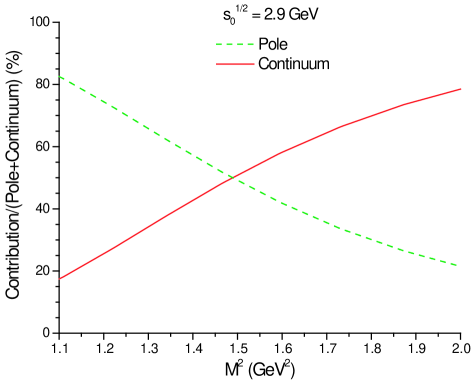
Figure 1: The dashed line shows the relative pole contribution (the pole contribution divided by the total, pole plus continuum, contribution) and the solid line shows the relative continuum contribution. The pole contribution should be bigger than the continuum, which happens for $M^{2}<1.5$ GeV² for $\sqrt{s_{0}}=2.9\nobreak\,\mbox{GeV}$.

The same analysis for the other values of the continuum threshold gives $M^{2}<1.4$ GeV² for $\sqrt{s_{0}}=2.7\nobreak\,\mbox{GeV}$ and $M^{2}<1.6$ GeV² for $\sqrt{s_{0}}=3.1\nobreak\,\mbox{GeV}$.

In Fig. 2, we show the $D_{s1}$ mass obtained from Eq. (12), in the $M^{2}$ region below the upper limit obtained above. We limit ourselves to the region $M^{2}>1.2~{}\nobreak\,\mbox{GeV}^{2}$ where the curves are more stable. Averaging the mass over all this region we get:

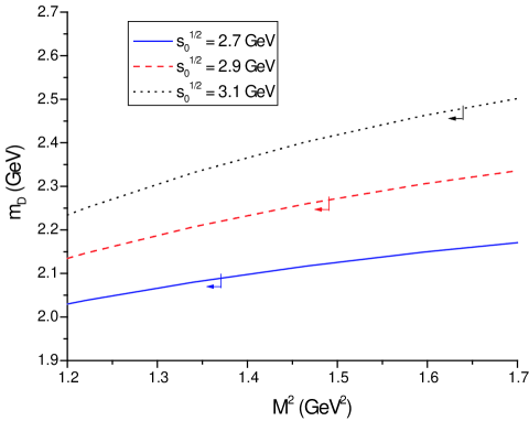
Figure 2: The $D_{s1}$ mass as a function of the sum rule parameter ($M^{2}$) for different values of the continuum threshold. The arrows indicate the region allowed by the upper limit imposed by the dominance of the QCD pole contribution.

$$m_{D_{s1}}=(2.3\pm 0.2)\nobreak\,\mbox{GeV}~{},$$ (13)

which is compatible with the experimental value $D_{s1}(2460)$ Swanson .

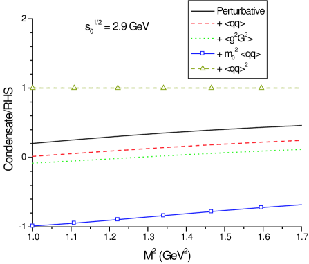
Figure 3: The OPE convergence in the region $1.0\leq M^{2}\leq 1.7~{}\nobreak\,\mbox{GeV}^{2}$ for $\sqrt{s_{0}}=2.9\nobreak\,\mbox{GeV}$. We start with the perturbative contribution and each subsequent line represents the addition of a condensate of higher dimension in the expansion.

II.2 OPE convergence

There is however a stronger constraint to the lower bound of the $M^{2}$ region. We have to analyze the convergence of the OPE by comparing the relative contribution of each term in Eqs. (7) to (11), to the right hand side of Eq. (6). The series converges better for higher values of $M^{2}$, so that requiring a good convergence sets a lower limit to $M^{2}$. This analysis in shown in figure 3.

Figure 3 shows no convergence in any region allowed by the upper bound given by pole/continuun analysis. This means that the lower bound given by OPE convergence will be higher than the upper bound, and there is no “sum rule window” where we can completely trust the results for this current.

The results above illustrate very well how we can reproduce the mass of a given state and then after a more carefult analysis conclude that the state is not a particle as such, being rather one of the possible continuum excitations.

III The scalar mesons

III.1 Light scalars

The same situation described in the last section is encountered in many sum rules with interpolating operators built with more than three quark fields. The light scalar meson interpolating operators used in ref. nosso.leves are:

$$j_{\sigma} = \epsilon_{abc}\epsilon_{dec}(u_{a}^{T}C\gamma_{5}d_{b})(\bar{u}_{d}\gamma_{5}C\bar{d}_{e}^{T}),$$

$$j_{f_{0}} = {\epsilon_{abc}\epsilon_{dec}\over\sqrt{2}}\left[(u_{a}^{T}C\gamma_{5}s_{b})(\bar{u}_{d}\gamma_{5}C\bar{s}_{e}^{T})+u\leftrightarrow d\right],$$

$$j_{a_{0}} = {\epsilon_{abc}\epsilon_{dec}\over\sqrt{2}}\left[(u_{a}^{T}C\gamma_{5}s_{b})(\bar{u}_{d}\gamma_{5}C\bar{s}_{e}^{T})-u\leftrightarrow d\right],$$

$$j_{\kappa} = \epsilon_{abc}\epsilon_{dec}(u_{a}^{T}C\gamma_{5}d_{b})(\bar{q}_{d}\gamma_{5}C\bar{s}_{e}^{T}),\;\;\;\bar{q}=\bar{u},\bar{d}.$$ (14)

They yield very low upper limits to $M^{2}$ when the pole and continuum contributions are analysed: $M^{2}<0.73\,\nobreak\,\mbox{GeV}^{2}$ for $a_{0}(980)$ and $f_{0}(980)$, $M^{2}<0.62\,\nobreak\,\mbox{GeV}^{2}$ for the $\kappa(800)$ and $M^{2}<0.54\,\nobreak\,\mbox{GeV}^{2}$ for the $\sigma(600)$.

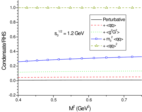
Figure 4: The $a_{0}(980)/f_{0}(980)$ OPE convergence in the region $0.4\leq M^{2}\leq 0.7~{}\nobreak\,\mbox{GeV}^{2}$ for $\sqrt{s_{0}}=1.2\nobreak\,\mbox{GeV}$.

The analysis was performed with the same parameters used in nosso.leves : $s_{0}^{\sigma}=1.0\,\nobreak\,\mbox{GeV}^{2}$, $s_{0}^{\kappa}=1.2\,\nobreak\,\mbox{GeV}^{2}$, $s_{0}^{f_{0}}=1.5\,\nobreak\,\mbox{GeV}^{2}$.

In figure 4 we show the OPE convergence for $a_{0}(980)$ and $f_{0}(980)$ (which have the same sum rule), in the same way shown in figure 3. In this figure we see that there is no OPE convergence in any region allowed by the upper bound. In fact, the situation of the light scalars is even worse than that of the $D_{s1}(2460)$, since the relative contribution of the dimension-6 condensate is even bigger. A possible reason for this is the fact that we are working with very small values for the Borel Mass ($M^{2}<1~{}\nobreak\,\mbox{GeV}^{2}$). As a matter of fact, once the integral on the right hand side of Eq. 5 is evaluated, the OPE side becomes a series with decreasing powers of $M^{2}$, which eventually become negative so that higher condensates will be divided by higher and higher powers of $M^{2}$. In the case of the tetraquarks the series begins with $M^{10}$ and one still has a positive power of $M^{2}$ for the dimension-8 condensate. However, it is hardly justifiable to truncate the series at this point since higher dimension condensates will be proportional to $(1/M^{2})^{{D-10\over 2}}$, where $D$ is the dimension of the condensate and for $M^{2}<1\nobreak\,\mbox{GeV}^{2}$ these condensates will not be suppressed, at least for $D\sim 10$.

It is interesting to notice that the authors of ref. cesa have arrived at the conclusion that the $a_{0}(980)$ scalar meson is not a four-quark state using a different criterion. The authors of ref. cesa have annalyzed the QCD sum rules of the $a_{0}(980)$ meson considered as a normal two-quark state, and also as a four-quark state. While they could reproduced both the mass and width of the $a_{0}(980)$ considered as a two-quark state, they were not able to reproduce the width of the $a_{0}(980)$ considered as a four-quark state.

It could be argued that these problems are related with the specific currents that we are working with, and that there could be other currents that might work better. In Ref. CHZ , five different interpolating operators for each of the light scalar mesons have been tested. In the case of the $\sigma$ these currents were:

$$S_{3}^{\sigma} = (u_{a}^{T}C\gamma_{5}d_{b})(\bar{u}_{a}\gamma_{5}C\bar{d}_{b}^{T}-\bar{u}_{b}\gamma_{5}C\bar{d}_{a}^{T}),$$

$$V_{3}^{\sigma} = (u_{a}^{T}C\gamma_{\mu}\gamma_{5}d_{b})(\bar{u}_{a}\gamma^{\mu}\gamma_{5}C\bar{d}_{b}^{T}-\bar{u}_{b}\gamma^{\mu}\gamma_{5}C\bar{d}_{a}^{T}),$$

$$T_{6}^{\sigma} = (u_{a}^{T}C\sigma_{\mu\nu}d_{b})(\bar{u}_{a}\sigma^{\mu\nu}C\bar{d}_{b}^{T}-\bar{u}_{b}\sigma^{\mu\nu}C\bar{d}_{a}^{T}),$$

$$A_{6}^{\sigma} = (u_{a}^{T}C\gamma_{\mu}d_{b})(\bar{u}_{a}\gamma^{\mu}C\bar{d}_{b}^{T}-\bar{u}_{b}\gamma^{\mu}C\bar{d}_{a}^{T}),$$

$$P_{3}^{\sigma} = (u_{a}^{T}Cd_{b})(\bar{u}_{a}C\bar{d}_{b}^{T}-\bar{u}_{b}C\bar{d}_{a}^{T}).$$ (15)

The currents for the other light scalars can be obtained by the following substitutions: $\kappa:(ud)(\bar{u}\bar{d})\rightarrow(ud)(\bar{d}\bar{s})$, $f_{0}:(ud)(\bar{u}\bar{d})\rightarrow(us)(\bar{u}\bar{s})+(ds)(\bar{d}\bar{s})$ and $a_{0}:(ud)(\bar{u}\bar{d})\rightarrow(us)(\bar{u}\bar{s})-(ds)(\bar{d}\bar{s})$. The authors of CHZ have tested all these currents and various linear combinations and found out that the better results were obtained with the particular combination: $\eta^{\sigma}_{1}=\mbox{cos}\theta A_{6}^{\sigma}+\mbox{sin}\theta V_{3}^{\sigma}$, with $\mbox{cos}\theta=1/\sqrt{2}$. They also obtain good results for the other light scalars with similar combinations.

We used the same analysis used above with the spectral densities obtained in CHZ and agree that the OPE convergence up to dimension 8 is quite good. On the other hand the pole dominance requirement imposes very low upper limits to $M^{2}$: $M^{2}<0.8\nobreak\,\mbox{GeV}^{2}$ for $a_{0}$ or $f_{0}$ ($\sqrt{s_{0}}=1.6\nobreak\,\mbox{GeV}$), $M^{2}<0.45\nobreak\,\mbox{GeV}^{2}$ for $\kappa$ ($\sqrt{s_{0}}=1.2\nobreak\,\mbox{GeV}$)and $M^{2}<0.35\nobreak\,\mbox{GeV}^{2}$ for $\sigma$ ($\sqrt{s_{0}}=1.\nobreak\,\mbox{GeV}$),

This means that the whole sum rule window lies below $M^{2}<1\nobreak\,\mbox{GeV}^{2}$ and, as commented above, it is at least dangerous to truncate the series at this order.

III.2 Charmed scalars

In the case of the charmed scalar $D_{s0}(2317)$, the current used for it in ref nosso.ds is:

$$j_{s} = {\epsilon_{abc}\epsilon_{dec}\over\sqrt{2}}\left[(u_{a}^{T}C\gamma_{5}c_{b})(\bar{u}_{d}\gamma_{5}C\bar{s}_{e}^{T})+u\leftrightarrow d\right].$$ (16)

If we require that the pole contribution be bigger than the continuum contribution we obtain $M^{2}<1.37\nobreak\,\mbox{GeV}^{2}$ for $\sqrt{s_{0}}=2.7\nobreak\,\mbox{GeV}$. In figure 5 we show the OPE convergence for the current (16) and we see that the OPE is still not convergent in the allowed region, as in the case of tme meson $D_{s1}(2460)$ studied in the previous section.

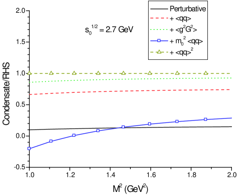
Figure 5: The $j_{s}$ OPE convergence in the region $1.0\leq M^{2}\leq 2.0~{}\nobreak\,\mbox{GeV}^{2}$ for $\sqrt{s_{0}}=2.7\nobreak\,\mbox{GeV}$.

IV Heavier tetraquarks

The situation improves as the quarks in the interpolating operator become heavier. In the case of the $X(3872)$, the following operator was used in ref. nosso.x :

$$j^{X}_{\mu} = {i\epsilon_{abc}\epsilon_{dec}\over\sqrt{2}}\bigg{[}(q_{a}^{T}C\gamma_{5}c_{b})(\bar{q}_{d}\gamma_{\mu}C\bar{c}_{e}^{T})+$$ (17)

$$+ (q_{a}^{T}C\gamma_{\mu}c_{b})(\bar{q}_{d}\gamma_{5}C\bar{c}_{e}^{T})].$$

The continuum contribution analysis for $j^{X}_{\mu}$ sets the upper limit at $M^{2}<2.6\,\nobreak\,\mbox{GeV}^{2}$ for a threshold of $\sqrt{s_{0}}=4.3\,\nobreak\,\mbox{GeV}$. The OPE convergence in this region is shown in figure 6.

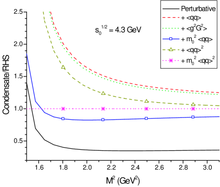
Figure 6: The $j^{X}_{\mu}$ OPE convergence in the region $1.5\leq M^{2}\leq 3.1~{}\nobreak\,\mbox{GeV}^{2}$ for $\sqrt{s_{0}}=4.3\nobreak\,\mbox{GeV}$.

We see that, for $M^{2}>1.9\nobreak\,\mbox{GeV}^{2}$, the addition of a subsequent term of the expansion brings the curve (representing the sum) closer to an asymptotic value (which was normalized to 1). Furthermore the changes in this curve become smaller with increasing dimension. These are the requirements for convergence and in this case we get a sum rule window in the region $1.9\nobreak\,\mbox{GeV}^{2}<M^{2}<2.6\nobreak\,\mbox{GeV}^{2}$. The mass obtained in nosso.x considering the allowed Borel window is

$$m_{X}=(3.92\pm 0.13)~{}\nobreak\,\mbox{GeV}\;,$$ (18)

which is compatible with the experimental value $X(3872)$.

A similar situation is found if we replace the $c$ quarks in Eq. (17) by $b$ quarks in order to predict the $X_{b}$ mass (as done in ref. nosso.x ). In this case the allowed Borel window is in the region $6.0\nobreak\,\mbox{GeV}^{2}<M^{2}<7.0\nobreak\,\mbox{GeV}^{2}$, and the predicted mass is

$$m_{X_{b}}=(10.14\pm 0.11)~{}\nobreak\,\mbox{GeV}\;,$$ (19)

which is in agreement with the findings in ref. guo .

From what was seen above we can conclude that for heavier tetraquarks the sum rules satisfy the validity criteria and hence allow the determination of the masses of these states. However, even in the present case we can not yet be very positive. Firstly because, as usual, the calculations might still be improved, with, for example, the inclusion of $\alpha_{s}$ corrections. Secondly because it remains very difficult to reproduce the $X$ narrow decay width, as shown in naniel . If the $X(3872)$ is proved to be a tetraquark state, it still remains to explain why we do not observe tetraquark states with charge different from $c\bar{c}$ states, such as $(cu)(\bar{c}\bar{d})$ or $(cd)(\bar{c}\bar{u})$ states, which would also have trustable QCDSR as the $X(3872)$. In this sense, the observation of a double charmed meson ($(cc)(\bar{q}\bar{q})$), which sum rule also obey all the convergence and pole dominance criteria tcc , would be very important to really determine the existence of tetraquark states.

V Conclusion

We have performed a QCD sum rules calculation of the $D_{s1}(2460)$ mass considering this state as a tetraquark and reanalized other recent similar tetraquark sum rules, giving special attention to the validity criteria of the method. We found that in the case of the lighter states, $\sigma(600)$, $\kappa(800)$, $a_{0}(980)$, $f_{0}(980)$ and also in the case of the intermediate $D_{s0}(2317)$ and $D_{s1}(2460)$ states, for the currents used in refs. nosso.leves ; nosso.ds , there are no values of the parameters $s_{0}$ and $M^{2}$ that satisfy all the desired conditions. In order to obtain results from the sum rules for these states we must abandon one or more of the conditions and choose the parameters arbitrarily.

When the interpolating operator is constructed with heavier quark fields the situation becomes better. We found suitable regions for the $X(3872)$ and its extension to the bottonic sector the $X_{b}$.

This problem was also present in the case of the pentaquarks MATTHEUS and seems connected to the high dimension of many-quark states interpolating operators, independently of the exact form of these operators. This may be an indication from the sum rules that light many-quark states can not be considered as ressonances separated from the continuum. Heavier many-quark states are supported by the sum rules in what concerns their masses. However it is very difficult (if possible) to explain their narrow decay widths.

While one might always argue that the so far existing calculations could be improved and the final conclusions might still change, to us at this point in time, this seems unlikely.

References

- (1) C. Amsler and N. Tornqvist, Phys. Rept. 389, 61 (2004), and references therein.
- (2) E. S. Swanson, Phys. Rept. 429, 243 (2006) and references therein.
- (3) R. L. Jaffe, Phys. Rev. D15, 267 (1977); R. L. Jaffe, hep-ph/0001123.
- (4) H. Suganuma, K. Tsumura, N. Ishii and F. Okiharu, PoS LAT2005, 070 (2006); hep-lat/0509121; F. Okiharu, H. Suganuma and T. T. Takahashi, Phys. Rev. D 72, 014505 (2005).
- (5) M.A. Shifman, A.I. and Vainshtein and V.I. Zakharov, Nucl. Phys. B147, 385 (1979).
- (6) L.J. Reinders, H. Rubinstein and S. Yazaki, Phys. Rep. 127, 1 (1985).
- (7) For a review and references to original works, see e.g., S. Narison, QCD as a theory of hadrons, Cambridge Monogr. Part. Phys. Nucl. Phys. Cosmol. 17, 1 (2002) [hep-h/0205006]; QCD spectral sum rules , World Sci. Lect. Notes Phys. 26, 1 (1989); Acta Phys. Pol. 26 (1995) 687; Riv. Nuov. Cim. 10N2 (1987) 1; Phys. Rept. 84, 263 (1982).
- (8) J. I. Latorre and P. Pascual, Jour. Phys. G11, L231 (1985); S. Narison, Phys. Lett. B175, 88 (1986).
- (9) T. V. Brito, F. S. Navarra, M. Nielsen, M. E. Bracco, Phys. Lett. B608, 69 (2005).
- (10) H-J. Lee and N.I. Kochelev, Phys. Lett. B642, 358 (2006); Z.-G. Wang, W.-M. Yang, S.-L. Wan, J .Phys. G31, 971 (2005); A. Zhang, Phys. Rev. D61, 114021 (2000); A. Zhang, T. Huang and T. Steele, hep-ph/0612146.
- (11) H.X. Chen, A. Hosaka and S.L. Zhu, hep-ph/0609163.
- (12) M. E. Bracco, A. Lozea, R. D. Matheus, F. S. Navarra, M. Nielsen, Phys. Lett. B624, 217 (2005).
- (13) H. Kim and Y. Oh, Phys. Rev. D72, 074012 (2005).
- (14) R. D. Matheus, S. Narison, M. Nielsen, J. M. Richard, Phys. Rev. D75, 014005 (2007).
- (15) M. Nielsen, Phys. Lett. B 634, 35 (2006).
- (16) F. S. Navarra and M. Nielsen, Phys. Lett. B 639, 272 (2006).
- (17) R. Matheus and S. Narison, Nucl. Phys (Proc. Suppl.) 152, 263 (2006).
- (18) R.D. Matheus, F. S. Navarra and M. Nielsen, Braz. J. Phys. 36, 1397 (2006).
- (19) Y. Kondo, O. Morimatsu and T. Nishikawa, Phys. Lett. B 611, 93 (2005); Y. Kwon, A. Hosaka and S. H. Lee, hep-ph/0505040.
- (20) H-J. Lee and N.I. Kochelev, Phys. Lett. B642, 358 (2006).
- (21) B.L. Ioffe, Nucl. Phys. B188, 317 (1981); B191, 591(E) (1981).
- (22) S. Narison, Phys. Lett. B466, 345 (1999).
- (23) C.A. Domingues and N. Paver, Z. Phys. C39, 39 (1988).
- (24) F.-K. Guo, P.-N. Shen, H.-C. Chiang and R.-G. Ping, Nucl. Phys. A761, 269 (2005).
- (25) F.S. Navarra, M. Nielsen and S.H. Lee, hep-ph/0703071.