Slow Convergence in Bootstrap Percolation

Abstract

In the bootstrap percolation model, sites in an $L$ by $L$ square are initially infected independently with probability $p$. At subsequent steps, a healthy site becomes infected if it has at least 2 infected neighbours. As $(L,p)\to(\infty,0)$, the probability that the entire square is eventually infected is known to undergo a phase transition in the parameter $p\log L$, occurring asymptotically at $\lambda=\pi^{2}/18$ [14]. We prove that the discrepancy between the critical parameter and its limit $\lambda$ is at least $\Omega((\log L)^{-1/2})$. In contrast, the critical window has width only $\Theta((\log L)^{-1})$. For the so-called modified model, we prove rigorous explicit bounds which imply for example that the relative discrepancy is at least $1\%$ even when $L=10^{3000}$. Our results shed some light on the observed differences between simulations and rigorous asymptotics.

1 Introduction

The standard bootstrap percolation model on the square lattice ${\mathbb{Z}}^{2}$ is defined as follows. For any set $K\subseteq{\mathbb{Z}}^{2}$ we define

$${\cal B}(K):=K\cup\big{\{}x\in{\mathbb{Z}}^{2}:\#\{y\in K:\|x-y\|_{1}=1\}\geq 2\big{\}},$$

and

$$\langle K\rangle:=\lim_{t\to\infty}{\cal B}^{t}(K),$$

where ${\cal B}^{t}$ denotes the $t$-th iterate of the function ${\cal B}$. The set $\langle K\rangle$ is the final set of infected sites if we start with $K$ infected.

Now fix $p\in(0,1)$ and let $W$ be a random subset of ${\mathbb{Z}}^{2}$ in which each site is included independently with probability $p$; more formally let ${\mathbb{P}}={\mathbb{P}}_{p}$ be the product measure with parameter $p$ on $\Omega=\{0,1\}^{{\mathbb{Z}}^{2}}$, and define the random variable $W=W(\omega):=\{x\in{\mathbb{Z}}^{2}:\omega(x)=1\}$ for $\omega\in\Omega$. We say that a set $K\subset{\mathbb{Z}}^{2}$ is internally spanned if $\langle K\cap W\rangle=K$. For $L\geq 1$ denote the square $R(L):=\{1,\ldots,L\}^{2}\subset{\mathbb{Z}}^{2}$. The main object of interest is the function

$$I(L)=I(L,p):={\mathbb{P}}_{p}\big{(}R(L)\text{ is internally spanned}\big{)}.$$

A central result is the following from [14].

• Theorem (phase transition, [14]) Consider the standard bootstrap percolation model. As $L\to\infty$ and $p\to 0$ simultaneously we have

  $$\begin{array}[]{rl}\text{if}\quad\liminf\,p\log L>\lambda&\text{then}\quad I(L,p)\to 1;\\ \text{if}\quad\limsup\,p\log L<\lambda&\text{then}\quad I(L,p)\to 0,\end{array}$$ (1)

  where $\lambda:={\pi^{2}}/{18}$.

Surprisingly, predictions for the asymptotic threshold $\lambda$ based on simulation differ greatly from the rigorous result. For example, in [2] the estimate $\lambda=0.245\pm 0.015$ is reported (based on simulation of squares up to size $L=28800$), whereas in fact $\lambda=\pi^{2}/18=0.548311\cdots$. This apparent discrepancy between theory and experiment has been investigated using partly non-rigorous methods in [8, 9, 18]. Our aim is to provide some rigorous understanding of the phenomenon. Our main result is the following strengthening of the first assertion in (1).

Theorem 1 (slow convergence)

Consider the standard bootstrap percolation model. There exists $c>0$ such that, if $L\to\infty$ and $p\to 0$ simultaneously in such a way that

$$p\log L>\lambda-\frac{c}{\surd\log L}\,,$$

where $\lambda=\pi^{2}/18$, then

$$I(L,p)\to 1.$$

(The condition in Theorem 1 may be equivalently expressed as $p\log L>\lambda-c^{\prime}\surd p$, for a different constant $c^{\prime}$). Thus, the convergence of the critical value of the parameter $p\log L$ to its limit $\lambda$ is very slow, with an asymptotic discrepancy of at least $c/\surd(\log L)$. (In order to halve the latter quantity, $L$ must be raised to the 4th power).

On the other hand, the window over which $I$ changes from near $0$ to near $1$ is much smaller – roughly $\mbox{constant}/\log L$. The precise statement depends on whether we vary $p$ or $L$, as follows.

For fixed $L$, and $\alpha\in(0,1)$, define $p_{\alpha}=p_{\alpha}(L):=\sup\{p:I(L,p)\leq\alpha\}$. Since $I(L,p)$ is continuous and strictly increasing in $p$, we have that $p_{\alpha}$ is the unique value such that $I(L,p_{\alpha})=\alpha$. The following was proved in [5] using a general result from [11].

• Theorem ($p$-window, [5]) Consider the standard bootstrap percolation model. For any fixed $\epsilon\in(0,1)$, we have

  $$p_{1-\epsilon}\log L-p_{\epsilon}\log L=O\bigg{(}\frac{\log\log L}{\log L}\bigg{)}=O\big{(}p_{1/2}\log p_{1/2}^{-1}\big{)}\quad\text{as }L\to\infty.$$ (2)

More precise estimates on the size of the window are available if we instead vary $L$. An upper bound was proved in [3]. Here we use similar methods to obtain matching upper and lower bounds. Since $I(L,p)$ is not necessarily monotone in $L$, we define for fixed $p$ and $\alpha\in(0,1)$: $\underline{L}_{\alpha}=\underline{L}_{\alpha}(p):=\min\{L:I(L,p)\geq\alpha\}$ and $\overline{L}_{\alpha}=\overline{L}_{\alpha}(p):=\max\{L:I(L,p)\leq\alpha\}$. Thus the interval $[\underline{L}_{\epsilon},\overline{L}_{1-\epsilon}]$ contains all those $L$ for which $I(L,p)\in[\epsilon,1-\epsilon]$.

Theorem 2 ($L$-window)

Consider the standard bootstrap percolation model. For any fixed $\epsilon\in(0,1/5)$, we have

$$p\log\overline{L}_{1-\epsilon}-p\log\underline{L}_{\epsilon}=\Theta(p)=\Theta\Big{(}1/{\log\overline{L}_{1/2}}\Big{)}\quad\text{as }p\to 0.$$

Indeed, for $p$ sufficiently small we have

$$p\log\overline{L}_{1-\epsilon}-p\log\underline{L}_{\epsilon}\in[C_{-}p,C_{+}p],$$

where $C_{\pm}=C_{\pm}(\epsilon)=(1/2\pm o(1))\log\epsilon^{-1}$ as $\epsilon\to 0$.

The modified bootstrap percolation model is a variant of the standard model in which we replace the update rule ${\cal B}$ with

$${\cal B}_{M}(K):=K\cup\big{\{}x\in{\mathbb{Z}}^{2}:\{x+e_{i},x-e_{i}\}\cap K\neq\emptyset\text{ for each of }i=1,2\big{\}}$$

(here $e_{1}:=(1,0)$ and $e_{2}:=(0,1)$ are the standard basis vectors), and define $\langle\cdot\rangle_{M}$, internally spanned, and $I_{M}(L,p)$ accordingly.

• Theorem ([14]) For the modified bootstrap percolation model, (1) holds with threshold $\lambda_{M}:=\pi^{2}/6$.

Theorem 3

Theorem 2 and (2) hold also for the modified model.

In the case of Theorem 1 we establish the following stronger version with an explicit error bound.

Theorem 4 (explicit bound)

For the modified model, if $p\leq 1/10$ and

$$p\log L\geq\lambda_{M}-\sqrt{2p}+{\cal E}(p),\quad\text{then}\quad I_{M}(L,p)\geq 1/2,$$

where $\lambda_{M}=\pi^{2}/6$ and ${\cal E}(p):=1.8p\log p^{-1}+2p$.

One may deduce rigorous numerical bounds such as the following.

Corollary 5

Consider the modified model. We have $p_{1/2}\log L<0.98\,\lambda_{M}$ when $L=10^{500}$, and $p_{1/2}\log L<0.99\,\lambda_{M}$ when $L=10^{3000}$.

• Proof. Take respectively $p=0.0014$ and $p=0.0002356$ in Theorem 4. $\Box$

Remarks

Aside from their mathematical interest, bootstrap percolation models have been applied to a variety of physical problems (see e.g. [1]), and as tools in the study of other models (e.g. [7, 10, 12]).

Several interesting attempts have been made to understand the discrepancy between simulation results (e.g. those of [2]) and the rigorous results in [14]; see e.g. [1, 8, 9, 18]. The present work is believed to be the first fully rigorous progress in this direction. In [18] it is estimated that $p_{1/2}\log L$ may become close to $\lambda=\pi^{2}/18$ only beyond about $L=10^{20}$ (the data given in [2] support a similar conclusion). Current simulations extend only to about $L=10^{5}$. A length scale of about $L=10^{10}$ is relevant to some physical applications. Thus it is important to understand this issue in more detail.

In particular, it would be of interest to determine the asymptotic behaviour of (say) $\lambda-p_{1/2}\log L$ as $L\to\infty$. Theorem 1 gives only a lower bound of $\Omega((\log L)^{-1/2})$. In [18] simulation data is fitted to $p_{1/2}\log L=\pi^{2}/18-0.45(\log L)^{-0.2}$. In [9], computer calculations together with a heuristic argument lead to the estimate $p_{1/2}\log L=\pi^{2}/6-3.67(\log L)^{-0.333}$ for the modified model.

The phenomenon of a critical window whose width is asymptotically much smaller than its distance from a limiting value has been proved in other settings including integer partitioning problems [6], but contrasts with more familiar models such as random graphs [17].

Outline of Proofs

The idea behind the phase transition result (1) from [14] is as follows. We expect the square $R(L)$ to be internally spanned if and only if it contains at least one internally spanned square of side $B\gg 1/p$, since with high probability this will grow indefinitely in the presence of a random background of density $p$. Such a square is sometimes called a nucleation centre or critical droplet. Therefore the critical regime should be roughly at $L^{2}I(B)\approx 1$, i.e. $\log L\approx(-\log I(B))/2$, and we need to estimate $I(B)$. First consider the modified model. One way for $R(B)$ to be internally spanned is for every square with its bottom left corner at $(1,1)$ to have at least one adjacent occupied site on each its top and right faces – then every such square will be internally spanned (we can think of an infected square growing from $R(1)$ to $R(B)$). A straightforward computation shows that the probability of this event is approximately $\exp[-2\lambda_{M}/p]$ where $\lambda_{M}=\pi^{2}/6$. This argument proves the first inequality in (1) for the modified model. (The second inequality requires a much more delicate argument - see [14]).

In order to prove the slow convergence result for the modified model, Theorem 4, we consider other ways for a square to be internally spanned. One way is for every site along the main diagonal to be occupied. For a square of size $A<p^{1/2}$, the latter event has higher probability than the event in the previous paragraph, because the probability of growing by one additional row and column is $p$ versus about $(Ap)^{2}$. Therefore let $A=p^{-1/2}/2$, and suppose $R(A)$ is internally spanned by this mechanism, while each square from $R(A)$ to $R(B)$ has occupied sites on its faces as before. By comparing the two growth mechanisms, we see that, compared with the previous argument, this increases the lower bound on $I(B)$ by a factor of least $[p/(Ap)^{2}]^{A}=\exp[Cp^{-1/2}]$. This argument therefore proves the analogue of Theorem 1 for the modified model. Theorem 4 is proved by a refinement of these ideas (see in particular Lemmas 15 and 17). The coefficient $\surd 2$ of $\surd p$ seems to be the best that can be achieved by this method.

The above argument cannot work for the standard bootstrap percolation model. This is because an internally spanned square can grow from a face whenever there is an occupied site within distance 2. Thus, each additional occupied site can allow growth by two rows or two columns, so we do not achieve sufficient saving by considering occupied sites along the diagonal. Instead we consider another mechanism. Rather than a growing square, we consider a growing rectangle which may change shape when it encounters vacant rows or columns. (Figure 1 illustrates the main idea). We may describe such growth by means of the path traced by the rectangle’s top right corner. As noted in [14], the probability of such a growth path becomes much smaller if it deviates far from the main diagonal (which corresponds to a growing square). However, it turns out that if the deviations are of scale only $p^{-1/2}$ then the “entropy factor” (the number of possible deviations) outweighs the “energy cost” (the reduction in probability for each path). This argument yields Theorem 1.

Notation

The following notation will be used throughout. For integers $a,b,c,d$ we denote the rectangle $(a,b;c,d):=([a,c]\times[b,d])\cap{\mathbb{Z}}^{2}$, and we write for convenience $R(m,n)=R(1,1;m,n)$ and $R(n)=R(n,n)$. The long side of a rectangle is $\mbox{\rm long}(R(a,b;c,d))=\max\{c-a+1,d-b+1\}$. A copy of a set $K\subseteq{\mathbb{Z}}^{2}$ is an image under an isometry of ${\mathbb{Z}}^{2}$. A site $x\in{\mathbb{Z}}^{2}$ is occupied if $x\in W$. A set of sites is vacant if it contains no occupied site.

It will sometimes be convenient to denote

$$q=q(p):=-\log(1-p),$$

and

$$f(z):=-\log(1-e^{-z}),$$

so that for any $K\subset{\mathbb{Z}}^{2}$,

$${\mathbb{P}}_{p}(K\text{ is not vacant})=1-(1-p)^{|K|}=\exp-f(|K|q).$$

Note that $q\geq p$, and $q\sim p$ as $p\to 0$. The function $f$ is positive, decreasing, and convex on $(0,\infty)$.

In Section 3 we will also have occasion to consider the functions

$$\beta(u):=\frac{u+\sqrt{u(4-3u)}}{2}\quad\text{and}\quad g(z):=-\log\beta(1-e^{-z}).$$

The thresholds $\lambda,\lambda_{M}$ arise from the integrals

$$\int_{0}^{\infty}f=\lambda_{M}=\frac{\pi^{2}}{6}\quad\text{and}\quad\int_{0}^{\infty}g=\lambda=\frac{\pi^{2}}{18}$$ (3)

(see [14]).

2 Critical Window

In this section we present a proof of Theorem 2, together with the extension to the modified model claimed in Theorem 3. The following lemma from [3] is useful.

Lemma 6

Let $R$ be a rectangle, and consider the standard or modified model. If $R$ is internally spanned then for every positive integer $k\leq\mbox{\rm long}(R)$ there exists an internally spanned rectangle $T\subseteq R$ with $\mbox{\rm long}(T)\in[k,2k]$.

• Proof. See [3]. $\Box$

Lemma 7 (comparison)

Consider the standard or modified model. For integers $L\geq\ell\geq 2$ and any $p\in(0,1)$ we have

• $$I(L)\geq\Big{(}1-e^{-I(\ell)\big{(}\tfrac{L}{\ell}-1\big{)}^{2}}\Big{)}\left(1-2L^{2}e^{-p\ell}\right);$$

• $$\left(1-2\ell^{2}e^{-p(\ell/4-1)}\right)I(L)\leq I(\ell)\bigg{(}\frac{2L}{\ell-1}\bigg{)}^{2}.$$

• Proof of Lemma 7(i). Let $m=\lfloor L/\ell\rfloor$, and consider the $m^{2}$ disjoint squares

  $$S_{k}=R(\ell)+k\ell,\qquad k\in\{0,\ldots,m-1\}^{d}.$$

  Let $E$ be the event that at least one of the $S_{k}$ is internally spanned, and let $F$ be the event that every copy of $R(1,\ell)$ in $R(L)$ is non-vacant. It is straightforward to see that if $E$ and $F$ both occur then $R(L)$ is internally spanned. Hence using the Harris-FKG inequality (see e.g. [13]),

  $$I(L)\geq{\mathbb{P}}(E){\mathbb{P}}(F)\geq \Big{(}1-(1-I(\ell))^{m^{2}}\Big{)}\Big{(}1-2L^{2}(1-p)^{\ell}\Big{)}$$

  $$\geq \Big{(}1-e^{-I(\ell)\big{(}\tfrac{L}{\ell}-1\big{)}^{2}}\Big{)}\left(1-2L^{2}e^{-p\ell}\right).$$

  $\Box$

• Proof of Lemma 7(ii). Let $s=\lfloor\ell/2\rfloor$ and $m=\lfloor L/s\rfloor$, and consider the $m^{2}$ overlapping squares

  $$S_{k}=R(\ell)+ks\wedge(L-\ell,L-\ell),\qquad k\in\{0,\ldots,m-1\}^{2},$$

  where $\wedge$ denotes coordinate-wise minimum. Note that $\bigcup_{k}S_{k}=R(L)$, and that the overlap between two adjacent squares has width at least $s$. It follows that any rectangle $T\subseteq R(L)$ with $\mbox{\rm long}(T)\leq s$ lies entirely within one of the $S_{k}$. Hence, using Lemma 6,

  $$I(L) \leq{\mathbb{P}}\left(\exists\text{ i.s. }T\subseteq R(L)\text{ with }\mbox{\rm long}(T)\in\big{[}\lfloor\tfrac{s}{2}\rfloor,s\big{]}\right)$$

  $$\leq{\mathbb{P}}\Big{[}\bigcup_{k}\big{\{}\exists\text{ i.s. }T\subseteq S_{k}\text{ with }\mbox{\rm long}(T)\in\big{[}\lfloor\tfrac{s}{2}\rfloor,s\big{]}\big{\}}\Big{]}$$

  $$\leq m^{2}{\mathbb{P}}\big{(}\exists\text{ i.s. }T\subseteq R(\ell)\text{ with }\mbox{\rm long}(T)\in\big{[}\lfloor\tfrac{s}{2}\rfloor,s\big{]}\big{)}.$$ (4)

  On the other hand, considering the event that every copy of $R(1,\lfloor\tfrac{s}{2}\rfloor)$ in $R(\ell)$ contains at least one occupied site, and using the argument from the proof of part (i), we have

  $$I(\ell)\geq{\mathbb{P}}\big{(}\exists\text{ i.s. }T\subseteq R(\ell)\text{ with }\mbox{\rm long}(T)\in\big{[}\lfloor\tfrac{s}{2}\rfloor,s\big{]}\big{)}\big{(}1-2\ell^{2}e^{-ps}\big{)}.$$

  Combining this with (4) yields the result. $\Box$

• Proof of Theorem 2. It follows from (1) that for any $\alpha\in(0,1)$ we have

  $$p\log\overline{L}_{\alpha}(p)\;,\;p\log\underline{L}_{\alpha}(p)\to\lambda\quad\text{as }p\to 0.$$ (5)

  Therefore, once the first equality is proved, the second follows immediately. To prove the first equality we will use Lemma 7 to derive upper and lower bounds on $p\log\overline{L}_{1-\epsilon}-p\log\underline{L}_{\epsilon}$.

  For the upper bound, we fix $\epsilon$ and use Lemma 7(i) with $L=\overline{L}_{1-\epsilon}(p)$ and $\ell=\underline{L}_{\epsilon}(p)$, noting that $I(L,p)\leq 1-\epsilon$ and $I(\ell,p)\geq\epsilon$. By (5), for $p$ sufficiently small (depending on $\epsilon$) we have $1-2L^{2}e^{-p\ell}\geq 1-\epsilon^{2}$, so we obtain for $p$ sufficiently small:

  $$1-\epsilon\geq\Big{(}1-e^{-\epsilon\big{(}\tfrac{\overline{L}_{1-\epsilon}}{\underline{L}_{\epsilon}}-1\big{)}^{2}}\Big{)}(1-\epsilon^{2}).$$

  Rearranging gives

  $$\frac{\overline{L}_{1-\epsilon}}{\underline{L}_{\epsilon}}\leq 1+\sqrt{\frac{1}{\epsilon}\log\frac{1+\epsilon}{\epsilon}},$$

  hence

  $$p\log\overline{L}_{1-\epsilon}-p\log\underline{L}_{\epsilon}\leq C_{+}p,$$

  where $C_{+}=\log\big{(}1+\sqrt{\epsilon^{-1}\log(\epsilon^{-1}+1)}\,\big{)}$ satisfies $C_{+}<\infty$ for all $\epsilon>0$ and $C_{+}\leq(\tfrac{1}{2}+o(1))\log\epsilon^{-1}$ as $\epsilon\to 0$.

  For the lower bound, we fix $\epsilon$ and use Lemma 7(ii) with $L=\overline{L}_{1-\epsilon}(p)+1$ and $\ell=\underline{L}_{\epsilon}(p)-1$, noting that $I(L,p)>1-\epsilon$ and $I(\ell,p)<\epsilon$. By (5), we have $2\ell^{2}e^{-p(\ell/4-1)}=o(1)$ as $p\to 0$, so we obtain:

  $$\big{(}1-o(1)\big{)}(1-\epsilon)\leq\epsilon\Big{(}\frac{2(\overline{L}_{1-\epsilon}+1)}{\underline{L}_{\epsilon}-2}\Big{)}^{2}.$$

  Rearranging gives

  $$\frac{\overline{L}_{1-\epsilon}+1}{\underline{L}_{\epsilon}-2}\geq\sqrt{\frac{(1-\epsilon)(1-o(1))}{4\epsilon}},$$

  as $p\to 0$. For $p$ sufficiently small we obtain

  $$p\log\overline{L}_{1-\epsilon}-p\log\underline{L}_{\epsilon}\geq C_{-}p,$$

  for any $C_{-}(\epsilon)<\log\sqrt{(1-\epsilon)/(4\epsilon)}$. Thus we may take $C_{-}>0$ for all $\epsilon<1/5$, and $C_{-}\geq(\tfrac{1}{2}-o(1))\log\epsilon^{-1}$ as $\epsilon\to 0$. $\Box$

3 Slow Convergence

The main step in proving Theorem 1 will be the following.

Proposition 8 (nucleation centres)

Consider the standard bootstrap percolation model. There exist $p_{0}>0$ and $c\in(0,\infty)$ such that, for all $p<p_{0}$ and $B\geq 2p^{-1}$,

$$I(B,p)\geq\exp\big{[}-2\lambda/p+c/\surd p\big{]},$$

where $\lambda=\pi^{2}/18$.

• Proof of Theorem 1. First suppose that $(L,p)\to(\infty,0)$ in such a way that for some $c_{1}$,

  $$p\log L>\lambda-c_{1}/\surd\log L.$$

  Then for $L$ sufficiently large we have in particular $p\log L>\lambda/2$, hence

  $$p\log L>\lambda-c_{2}\surd p,$$ (6)

  where $c_{2}=2c_{1}/\lambda$.

  Therefore it is enough to prove that for some $c_{2}>0$, if $(L,p)\to(\infty,0)$ satisfy (6) then $I(L,p)\to 1$. Furthermore, we may assume that we have equality in (6), since if not we may find (for $p$ sufficiently small) $p^{\prime}<p$ such that $p^{\prime}\log L=\lambda-c_{2}\surd p^{\prime}$, and then $I(L,p)\geq I(L,p^{\prime})\to 1$. Therefore let

  $$L=\exp\Big{[}\lambda/p-c_{2}/\surd p\Big{]}\quad\text{and}\quad B=\lceil p^{-3}\rceil.$$

  Using Lemma 7(i),

  $$I(L)\geq\Big{(}1-e^{-I(B)\big{(}\tfrac{L}{B}-1\big{)}^{2}}\Big{)}\left(1-2L^{2}e^{-pB}\right).$$ (7)

  Proposition 8 and the above definition of $L$ easily imply $L^{2}e^{-pB}\to 0$ as $p\to 0$, while

  $$\log\Big{[}I(B)(L/B-1)^{2}\Big{]}\leq-2\lambda/p+c/\surd p+2\big{(}\lambda/p-c_{2}/\surd p\big{)}+O(\log p^{-1})\to 0$$

  as $p\to 0$ provided $2c_{2}>c$. Then (7) gives $I(L,p)\to 1$ as required. $\Box$

In order to prove Proposition 8 we consider various ways for $R(B)$ to be internally spanned. The simplest way involves symmetric growth starting from a corner. We say that a sequence of events $A_{1},A_{2},\ldots,A_{k}$ has a double gap if there is a consecutive pair $A_{i},A_{i+1}$ neither of which occur. For integers $2\leq a\leq b$, let ${\cal D}_{a}^{b}$ be the event that:

$$\big{\{}R(1,i;\;i-2,i)\text{ is not vacant}\big{\}}_{i=a+1,\ldots,b}$$ has no double gaps, and

$$\big{\{}R(i,1;\;i,i-2)\text{ is not vacant}\big{\}}_{i=a+1,\ldots,b}$$ has no double gaps.

See Figure 1(i). Note that if $R(a)$ is internally spanned, and ${\cal D}_{a}^{b}$ occurs, then $R(s,t)$ is internally spanned for some $s,t\in\{b-1,b\}$. Indeed, it is easily seen that we may find a sequence of internally spanned rectangles $R(i,j)$ with $|i-j|\leq 2$, starting with $R(a)$ and ending with $R(s,t)$, with the width or the height increasing by 1 or 2 at each step.

Figure 1: Two possible mechanisms for growth from $R(a)$ to $R(b)$. (i) The event ${\cal D}_{a}^{b}$: no two consecutive strips are vacant. (ii) The event ${\cal J}_{a}^{b}$: the gray strips are non-vacant, the hatched region is vacant, the black site is occupied, and the horizontal/vertical arrows indicate no two consecutive vacant columns/rows respectively.

We will also consider the following alternative growth mechanism. For positive integers $a\leq b-4$, let ${\cal J}_{a}^{b}$ be the event that:

$$R(1,a+1;\;a-1,a+1) \text{ is not vacant},$$

$$R(a+1,1;\;a+1,a-1) \text{ is not vacant},$$

$$\big{\{}R(i,1;\;i,a+1)\text{ is not vacant}\big{\}} {}_{i=a+2,\ldots,b-1}\text{ has no double gaps},$$

$$(b,1;\;b,a+1) \text{ is not vacant},$$

$$R(1,a+2;\;b-1,a+3) \text{ {\em is} vacant},$$

$$(b,a+3) \text{ is occupied},$$

$$\big{\{}R(1,i;\;b,i)\text{ is not vacant}\big{\}} {}_{i=a+4,\ldots,b-1}\text{ has no double gaps, and}$$

$$R(1,b;\;b,b) \text{ is not vacant}.$$

See Figure 1(ii). Note again that if $R(a)$ is internally spanned and ${\cal J}_{a}^{b}$ occurs then $R(b)$ is internally spanned. In this case, vertical growth is stopped by the two vacant rows, and there is a sequence of horizontally growing internally spanned rectangles, followed by vertical growth after the occupied site $(b,a+3)$ is encountered.

Now fix a positive integer $B$. For positive integers $(a_{i},b_{i})_{i=1,\ldots,m}$ satisfying $2\leq a_{1}\leq b_{1}\leq a_{2}\leq\cdots\leq b_{m}\leq B$ and $b_{i}-a_{i}\leq 4\;\forall i$, define the event

$${\cal E}(a_{1},b_{1},\ldots,a_{m},b_{m}) :={\cal D}_{2}^{a_{1}}\cap\Big{(}\bigcap_{i=1}^{m}{\cal J}_{a_{i}}^{b_{i}}\Big{)}\cap\Big{(}\bigcap_{i=1}^{m-1}{\cal D}_{b_{i}}^{a_{i+1}}\Big{)}\cap{\cal D}_{b_{m}}^{B-1}$$

$$\cap\Big{\{}(1,1),(2,2),(B,1),(1,B)\text{ are occupied}\Big{\}}.$$

Lemma 9 (properties of ${\cal E}$)

• The various events appearing in the above definition of ${\cal E}(a_{1},\ldots,b_{m})$ are independent.

• If ${\cal E}(a_{1},\ldots,b_{m})$ occurs then $R(B)$ is internally spanned.

• For different choices of $a_{1},\ldots,b_{m}$, the events ${\cal E}(a_{1},\ldots,b_{m})$ are disjoint.

• Proof. Property (i) is clear from the definitions of the ${\cal D}$ and ${\cal J}$ events. Property (ii) follows from the earlier remarks on these events: indeed the squares $R(2),R(b_{1}),\ldots,R(b_{m}),R(B)$ are all internally spanned. To see (iii), fix a configuration and consider examining in sequence the rows $R(1,i;\;i-2,i)$ for $i=3,4,5,\ldots$. The presence of two consecutive vacant rows signals an event ${\cal J}_{a}^{b}$, and determines the value of $a$, and then if we follow the upper vacant row to the right until an occupied site is encountered, we discover the corresponding value of $b$. $\Box$

We will obtain a lower bound on the probability $R(B)$ is internally spanned by bounding the probability of each event ${\cal E}$ (for certain choices of the $a_{i},b_{i}$), and bounding the number of possible choices.

We start by estimating the probability of ${\cal D}_{a}^{b}$, for which we need the following slight refinement of a result from [14] (see [4] for a much more precise result in the same direction). Recall the function $\beta$ defined in the introduction.

Proposition 10 (double gaps)

For independent events $A_{1},\ldots,A_{k}$ whose probabilities $u_{i}:={\mathbb{P}}(A_{i})$ form an increasing or decreasing sequence, the probability that there are no double gaps is at least $\prod_{i=1}^{k}\beta(u_{i})$.

Lemma 11

For $0\leq u\leq v\leq 1$ we have $u\beta(v)+(1-u)v\geq\beta(u)\beta(v)$.

• Proof. The function $h(u,v):=u\beta(v)+(1-u)v-\beta(u)\beta(v)$ satisfies $h(v,v)=0$, so it suffices to show that $h$ is decreasing in $u$ for $u\leq v$. But we have $\partial h/\partial u=\beta(v)-v-\beta^{\prime}(u)\beta(v)\leq 0$, by the elementary computations $\beta^{\prime}(u)\geq\beta^{\prime}(v)\geq(\beta(v)-v)/\beta(v)$. $\Box$

• Proof of Proposition 10. Without loss of generality suppose the probabilities $u_{i}$ are decreasing. Let $a_{k}$ be the probability that the sequence $A_{1},\ldots,A_{k}$ has no double gaps. Then $a_{0}=a_{1}=1$, and by conditioning on the last two events we obtain $a_{k}=u_{k}a_{k-1}+(1-u_{k})u_{k-1}a_{k-2}$. The result follows by induction, using Lemma 11 thus: $a_{k}\geq[u_{k}\beta(u_{k-1})+(1-u_{k})u_{k-1}]\prod_{i=1}^{k-2}\beta(u_{i})\geq\prod_{i=1}^{k}\beta(u_{i})$. $\Box$

Recall the function $g$ from the introduction, and write for $a\leq b$,

$$G_{a}^{b}=G_{a}^{b}(p):=\exp\Big{[}\textstyle-\sum_{i=a}^{b-1}g(iq)\Big{]}.$$

Lemma 12 (diagonal growth)

$${\mathbb{P}}_{p}({\cal D}_{a}^{b})\geq(G_{a-1}^{b-1})^{2}$$

• Proof. Immediate from Proposition 10 and the definitions of ${\cal D}_{a}^{b}$ and $g$. $\Box$

Next we estimate the relative cost of a ${\cal J}$-event.

Lemma 13 (deviation cost)

Fix positive constants $c_{-}<c_{+}$. For any $p\in(0,1/2)$ and $a\leq b-4$ satisfying $a,b\in[c_{-}/p,c_{+}/p]$, we have

$$\frac{{\mathbb{P}}_{p}({\cal J}_{a}^{b})}{(G_{a-1}^{b-1})^{2}}\geq Cp\,e^{-C^{\prime}p(b-a)^{2}},$$

where $C,C^{\prime}\in(0,\infty)$ depend only on $c_{\pm}$.

• Proof. From the definition of ${\cal J}_{a}^{b}$ and Proposition 10 we obtain

  $${\mathbb{P}}_{p}({\cal J}_{a}^{b})\geq[1-(1-p)^{a}]^{4}(1-p)^{2b}\,p\,\exp\big{[}-(b-a)g(aq)-(b-a)g(bq)\big{]}.$$

  Note that $g$ is decreasing, and that $(1-p)^{k}$ is bounded away from 0 and 1 for $k\in[c_{-}/p,c_{+}/p]$, so we deduce

  $${\mathbb{P}}_{p}({\cal J}_{a}^{b})\geq Cp\,\exp\big{[}-2(b-a)g(aq)\big{]}.$$ (8)

  Also we have

  $$(G_{a-1}^{b-1})^{2}=\exp\big{[}\textstyle-2\sum_{i=a-1}^{b-2}g(iq)\big{]}\leq\exp\big{[}-2(b-a)g(bq)\big{]}.$$ (9)

  Now $g(aq)-g(bq)\leq(bq-aq)\max_{z\in[aq,bq]}|g^{\prime}(z)|$, but the ratio $q/p$ is bounded for $p<1/2$, hence $g^{\prime}$ is uniformly bounded over the relevant interval, and we obtain $g(aq)-g(bq)\leq C^{\prime}(b-a)p$. Therefore dividing (8) by (9) gives the result. $\Box$

• Proof of Proposition 8. Let $m=\lfloor Mp^{-1/2}\rfloor$, where $M<1/4$ is a constant to be chosen later. Suppose integers $(a_{i},b_{i})_{i=1,\ldots,m}$ and $B$ satisfy:

  $$\begin{array}[]{c}p^{-1}<a_{1}\leq b_{1}\leq a_{2}\leq\cdots\leq b_{m}<2p^{-1}\leq B\\ b_{i}-a_{i}\in[4,p^{-1/2}]\qquad\forall i\end{array}$$ (10)

  Let $C,C^{\prime}$ be the constants from Lemma 13 corresponding to $c_{-}=1$ and $c_{+}=2$. Then from the definition of the event ${\cal E}$ together with Lemmas 9(i), 12 and 13 we obtain:

  $${\mathbb{P}}_{p}\big{[}{\cal E}(a_{1},\ldots,b_{m})\big{]} \geq p^{4}\big{[}Cp\,e^{-C^{\prime}p(p^{-1/2})^{2}}\big{]}^{m}\exp\big{[}\textstyle-2\sum_{i=1}^{B-1}g(iq)\big{]}$$

  $$=p^{4}(C^{\prime\prime}p)^{m}(G_{1}^{B})^{2}$$ (11)

  for $C^{\prime\prime}$ a fixed constant. Now since $mp^{-1/2}<p^{-1}/4$, the number of possible choices of $(a_{i},b_{i})_{i=1,\ldots,m}$ satisfying (10) is at least

  $${{\lfloor p^{-1}-mp^{-1/2}\rfloor}\choose m}(p^{-1/2}-4)^{m}\geq\frac{(p^{-1}/2)^{m}}{m^{m}}(p^{-1/2}/2)^{m}=\Big{(}\frac{1}{4pM}\Big{)}^{m}$$ (12)

  for $p$ sufficiently small.

  By Lemma 9(ii),(iii) we may multiply (11) and (12) to give for $p$ sufficiently small and all $B>2p^{-1}$,

  $$I(B)\geq p^{4}\Big{(}\frac{C^{\prime\prime}}{4M}\Big{)}^{m}(G_{1}^{B})^{2}.$$

  Now choose $M=C^{\prime\prime}/8$ (recall that $C^{\prime\prime}$ was an absolute constant) so that $C^{\prime\prime}/4M=2$. Also note that since $g$ is decreasing,

  $$-\log G_{1}^{B}=\sum_{i=1}^{B-1}g(iq)\leq q^{-1}\int_{0}^{Bq}g\leq p^{-1}\int_{0}^{\infty}g=p^{-1}\lambda.$$

  Hence for $p$ sufficiently small,

  $$I(B)\geq p^{4}2^{Mp^{-1/2}/2}\exp[-2p^{-1}\lambda]\geq\exp[-2p^{-1}\lambda+cp^{-1/2}],$$

  as required. $\Box$

4 Explicit bound for the modified model

In this section we prove Theorem 4. Since we always refer to the modified model we sometimes omit the subscript $M$ in $I_{M}$.

Proposition 14 (nucleation centres)

Consider the modified model. For any $p\leq 1/10$ and any $B\geq\sqrt{2/p}$ we have

$$I(B)\geq\exp\Big{[}-2\lambda_{M}/q+2\sqrt{2/p}-\log p^{-1}-3.2\Big{]},$$

where $\lambda_{M}=\pi^{2}/6$.

Lemma 15 (diagonal spanning)

For the modified model we have for any positive integer $a$ and any $p\in(0,1)$,

$$I_{M}(a)\geq\tfrac{1}{2}\left(2p-p^{2}\right)^{a}.$$

• Proof. Note that for $a\geq 2$, the square $R(a)$ is internally spanned provided $(1,1)$ is occupied and $R(2,2;a,a)$ is internally spanned, or alternatively provided $(1,a)$ is occupied and $R(2,1;a,a-1)$ is internally spanned. Hence

  $$I(a)\geq pI(a-1)+(1-p)pI(a-1)=(2p-p^{2})I(a-1).$$

  The result follows by induction. $\Box$

Denote

$$F_{a}^{b}=F_{a}^{b}(p):=\textstyle\prod_{j=a}^{b-1}\big{(}1-(1-p)^{j})=\exp\Big{[}\textstyle-\sum_{i=a}^{b-1}f(iq)\Big{]}.$$

Lemma 16 (growth)

Let $a\leq b$ be integers and let $p\in(0,1)$. For the standard or modified model, we have

$$I(b)\geq I(a)(F_{a}^{b})^{2}.$$

• Proof. Let $F$ be the event that each of the strips

  $$R(j+1,1;\;j+1,j),\qquad j=a,a+1,\ldots,b,$$

  $$R(1,j+1;\;j,j+1),\qquad j=a,a+1,\ldots,b$$

  is non-vacant. It is easily seen that if $R(a)$ is internally spanned and $F$ occurs then $R(b)$ is internally spanned. Hence

  $$I(b)\geq{\mathbb{P}}(\{R(a)\text{ is i.s.}\}\cap F)=I(a){\mathbb{P}}(F)=I(a)(F_{a}^{b})^{2}.$$

  $\Box$

We next note some elementary bounds. We have

$$p\leq q\leq p+p^{2},$$ (13)

where the second inequality holds provided $p<1/2$. The function $F_{a}^{b}$ satisfies

$$\exp\bigg{[}-\frac{1}{q}\int_{(a-1)q}^{(b-1)q}f\bigg{]}\leq F_{a}^{b}\leq\exp\bigg{[}-\frac{1}{q}\int_{aq}^{bq}f\bigg{]},$$ (14)

since $f$ is decreasing.

Also note the inequalitites

$$\log\epsilon^{-1} \leq f(\epsilon)\leq\log\epsilon^{-1}+\epsilon$$ (15)

$$e^{-K} \leq f(K)\leq e^{-K}+e^{-2K},$$ (16)

where the fourth inequality holds provided $K>1/2$. (The inequalities are useful when $\epsilon\ll 1\ll K$). Hence

$$\epsilon\log\epsilon^{-1}+\epsilon \leq\int_{0}^{\epsilon}f\leq\epsilon\log\epsilon^{-1}+\epsilon+\tfrac{1}{2}\epsilon^{2}$$ (17)

$$e^{-K} \leq\int_{K}^{\infty}f\leq e^{-K}+\tfrac{1}{2}e^{-2K},$$ (18)

where the fourth inequality holds provided $K>1/2$.

• Proof of Proposition 14. Fix $p<1/10$, and let $A\leq B$ be positive integers (later we will take $A\approx\sqrt{2/p}$).

  By Lemmas 15 and 16 we have

  $$I(B)\geq\tfrac{1}{2}(2p-p^{2})^{A}(F_{A}^{B})^{2},$$

  so using (14), (3) and (17), and rearranging,

  $$\log I(B)\geq-\log 2+A\log(2p-p^{2})-\frac{2}{q}\int_{(A-1)q}^{\infty}f$$

  $$\geq-\log 2+A\log(2p-p^{2})-\frac{2}{q}\Big{(}\lambda_{M}-(A-1)q\log[(A-1)q]^{-1}-(A-1)q\Big{)}$$

  $$=-\frac{2\lambda_{M}}{q}+2(A-1)\log\frac{e\sqrt{2}}{(A\!-\!1)\sqrt{p}}+2(A-1)\log\frac{p}{q}+A\log(1-\frac{p}{2})+\log p,$$

  where we have written $(2p-p^{2})=2p(1-p/2)$. By (13), for $p<1/2$ we have $\log(p/q)\geq\log[p/(p+p^{2})]=-\log(1+p)\geq-p$, and $\log(1-p/2)\geq-p/2-p^{2}/4$, so we obtain

  $$\log I(B)\geq-\frac{2\lambda_{M}}{q}+2(A-1)\log\frac{e\sqrt{2}}{(A-1)\sqrt{p}}-2(A-1)p-A(p/2+p^{2}/4)+\log p.$$

  Now let

  $$A=\big{\lceil}\sqrt{2/p}\big{\rceil},$$

  to give for $p\leq 1/10$ and $B\geq A$,

  $$\log I(B)$$

  $$\geq-\frac{2\lambda_{M}}{q}+2\big{(}\sqrt{2/p}-1\big{)}1-2\sqrt{2/p}\;p-\big{(}\sqrt{2/p}+1)(p/2+p^{2}/4)+\log p$$

  $$\geq-\frac{2\lambda_{M}}{q}+\frac{2\surd 2}{\surd p}-\log p^{-1}-3.2.$$

  Note the non-trivial cancelation between terms in $p^{-1/2}\log p^{-1}$. $\Box$

The following variant of Lemma 7(i) allows better control of the error terms.

Lemma 17 (scanning estimate)

Let $b,\ell,m$ positive integers with $mb<\ell$, and let $p\in(0,1)$. For the standard or modified model, we have

$$I(\ell)\geq\left(1-e^{-m^{2}I(b)}\right)(F_{b}^{\ell}F_{\ell-mb}^{\ell})^{2}\big{(}1-(1-p)^{\ell-mb}\big{)}^{\ell}.$$

• Proof. Consider the $m^{2}$ disjoint squares

  $$S_{k}:=R(b)+bk,\qquad k\in\{0,\ldots,m-1\}^{2},$$

  and let

  $$\{0,\ldots,m-1\big{\}}^{2}=\big{\{}k(1),k(2),\ldots,k(m^{2})\big{\}}$$

  be the lexicographic ordering of the set on the left side. For $i=1,\ldots,m^{2}$ define the event

  $$J_{i}=\{S_{k(i)}\text{ is internally spanned}\},$$

  and let $F_{i}$ be the event that each of the strips

  $$R(\ell)\cap[bk(i)+R(j+1,1;\;j+1,j)],\qquad j=b,b+1,\ldots$$

  $$R(\ell)\cap[bk(i)+R(1,j+1;\;j,j+1)],\qquad j=b,b+1,\ldots$$

  that is non-empty is non-vacant. See Figure 2. Also define the event

  $$E=\big{\{}\langle W\cap R(\ell)\rangle\supseteq R(mb+1,mb+1;\;\ell,\ell)\big{\}}.$$

  It is straightforward to see that for any $i$, if $J_{i}$ and $F_{i}$ occur then $E$ occurs. Furthermore, for each $i$, the event $F_{i}$ is independent of the events $J_{1},\ldots,J_{i}$.

  

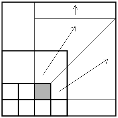
  Figure 2: An illustration of the proof of Lemma 17. Here $m=4$, and the first internally spanned sub-square is $S_{k(7)}=S_{(2,1)}$. The arrows indicate the event $F_{7}$.

Hence we have

$${\mathbb{P}}(E) \geq{\mathbb{P}}\bigg{[}\bigcup_{i=1}^{m^{2}}\big{(}J_{1}^{C}\cap\cdots\cap J_{i-1}^{C}\cap J_{i}\cap F_{i}\big{)}\bigg{]}$$

$$=\sum_{i=1}^{m^{2}}{\mathbb{P}}\big{(}J_{1}^{C}\cap\cdots\cap J_{i-1}^{C}\cap J_{i}\big{)}{\mathbb{P}}(F_{i})$$

$$\geq{\mathbb{P}}(J_{1}\cup\cdots\cup J_{m^{2}})\min_{i}{\mathbb{P}}(F_{i})$$

$$\geq\left(1-e^{-m^{2}I(b)}\right)(F_{b}^{\ell})^{2}\big{(}1-(1-p)^{\ell-mb}\big{)}^{\ell}.$$ (19)

To conclude, let $H$ be the event that each of the strips

$$R(j,j-1;\;j,\ell),\qquad j=mb,\ldots,2,1$$

$$R(j-1,j;\;\ell,j),\qquad j=mb,\ldots,2,1$$

is non-vacant. Using the Harris-FKG inequality we have $I(\ell)\geq{\mathbb{P}}(E\cap H)\geq{\mathbb{P}}(E){\mathbb{P}}(H)\geq{\mathbb{P}}(E)(F_{\ell-mb}^{\ell})^{2}$, and combining this with (19) gives the result. $\Box$

• Proof of Theorem 4. Fix $p\leq 10$ and let $B\geq\sqrt{2/p}$, and take $L$ and $m$ such that $L\geq mB$. We use Lemma 17 to derive a lower bound for $I(L)$. We obtain

  $$I(L)\geq\Big{(}1-e^{-m^{2}I(B)}\Big{)}(F_{B}^{\infty}F_{L-mB}^{\infty})^{2}e^{-Lf([L-mB]q)}.$$ (20)

  Consider the first factor above. Take

  $$m=\left\lceil\exp\bigg{(}\frac{\lambda_{M}}{q}-{\frac{\surd 2}{\surd p}}+\frac{1}{2}\log p^{-1}+1.8\bigg{)}\right\rceil.$$ (21)

  Then Proposition 14 implies $\log(m^{2}I(B))\geq 0.4$, and therefore

  $$1-e^{-m^{2}I(B)}\geq 1-e^{-e^{0.4}}.$$

  Turning to the other factors in (20), we have by (14),

  $$(F_{B}^{\infty}F_{L-mB}^{\infty})^{2}e^{-Lf([L-mB]q)}$$

  $$\geq \exp\Big{(}-\frac{2}{q}\int_{(B-1)q}^{\infty}f-\frac{2}{q}\int_{(L-mB-1)q}^{\infty}f-Lf([L-mb]q)\Big{)}$$

  $$\geq 1-\frac{2}{q}\int_{(B-1)q}^{\infty}f-\frac{2}{q}\int_{(L-mB-1)q}^{\infty}f-Lf([L-mb]q).$$

  We now set

  $$B=1+\Big{\lceil}\frac{3+\log q^{-1}}{q}\Big{\rceil}\quad\text{and}\quad L=mB+4cq^{-2},$$ (22)

  for any $c\geq 1$. It is straightforward to check that for $p\leq 1/10$ we have $(L-mB-1)q>(B-1)q>1/2$, so we may use (16),(18) to bound the above terms thus:

  $$\frac{2}{q}\int_{(B-1)q}^{\infty}f-\frac{2}{q}\int_{(L-mB-1)q}^{\infty}f\leq\frac{4}{q}\Big{(}e^{-(B-1)q}+e^{-2(B-1)q}\Big{)}\leq 4e^{-3}+4e^{-6},$$

  and

  $$Lf([L-mb]q)\leq 2Le^{-(L-mB)q}\leq 2\big{(}e^{2/q}2q^{-2}+4cq^{-2}+1)e^{-4c/q}\\ \leq 2(e^{2/q}2q^{-2}+4q^{-2}+1)e^{-4/q}\leq e^{-2}$$

  since $m\leq e^{2/q}$ and $B\leq 2q^{-2}$ for $p\leq 1/10$. Hence, returning to (20), for the given choices of $B,L$ we have

  $$I(L)\geq(1-e^{-e^{0.4}})(1-4e^{-3}-4e^{-6}-e^{-2})>1/2.$$

  From (22) we have shown that $I(L,p)>1/2$ provided $p\leq 1/10$ and

  $$p\log L\geq p\log(mB+4q^{-2})=p\log m+p\log B+p\log\Big{(}1+\frac{4q^{-2}}{mB}\Big{)}.$$ (23)

  Finally we need to find upper bounds for the terms appearing on the right of (23). By (21) we have

  $$p\log m\leq\lambda_{M}\frac{p}{q}-\sqrt{2p}+\frac{1}{2}p\log p^{-1}+1.8p+p\log\frac{m}{m-1}.$$

  But for $p\leq 1/10$ we have $p\log(m/(m-1))=-p\log(1-1/m)\leq 2p/m\leq 2pe^{-1/p}\leq 0.001p$, while $p/q\leq p/(p+p^{2}/2)\leq 1-0.47p$, so

  $$p\log m\leq\lambda_{M}-\sqrt{2p}+\frac{1}{2}p\log p^{-1}+1.03p.$$

  By (22) we have

  $$p\log B\leq p\log\Big{(}2+\frac{3}{q}+\frac{\log q^{-1}}{q}\Big{)}\leq p\log(2.6p^{-1.3})=0.96p+1.3p\log p^{-1}.$$

  Since $4q^{-2}>B$ and $m\geq e^{1/p}$ for $p\leq 1/10$, we have

  $$p\log\Big{(}1+\frac{4q^{-2}}{mB}\Big{)}\leq pe^{-1/p}\leq 0.001p.$$

  Hence the right side of (23) is at most

  $$\lambda_{M}-\sqrt{2p}+1.8p\log p^{-1}+2p,$$

  as required. $\Box$

Open Problems

• Prove a complementary bound to Theorem 1. For example, do there exist $\gamma,c<(0,\infty)$ such that $(L,p)\to(\infty,0)$ with $p\log L<\lambda-c(\log L)^{-\gamma}$ implies $I\to 0$?

• Prove matching upper and lower bounds, e.g. involving inequalities of the form $p\log L\lessgtr\lambda-c(\log L)^{\gamma\pm\epsilon}$, or even $p\log L\lessgtr\lambda-(c\pm\epsilon)F(L)$.

• Extend the results to other bootstrap percolation models for which sharp thresholds are known to exist – currently those in [15, 16].

• Identify more precisely the width of the critical window as $p$ varies. Is it the case that $p_{1-\epsilon}\log L-p_{\epsilon}\log L=\Theta(1/\log L)$ as $L\to\infty$?

Alexander E. Holroyd: holroyd(at)math.ubc.ca
Department of Mathematics, University of British Columbia,
121-1984 Mathematics Rd, Vancouver, BC V6T 1Z2, Canada

Janko Gravner: gravner(at)math.ucdavis.edu
Mathematics Department, University of California,
Davis, CA 95616, USA

References

[1]
J. Adler and U. Lev.
Bootstrap percolation: Visualizations and applications.
Brazillian J. Phys., 33(3):641–644, 2003.
[2]
J. Adler, D. Stauffer, and A. Aharony.
Comparison of bootstrap percolation models.
J. Phys. A, 22:L297–L301, 1989.
[3]
M. Aizenman and J. L. Lebowitz.
Metastability effects in bootstrap percolation.
J. Phys. A, 21(19):3801–3813, 1988.
[4]
G. E. Andrews.
Partitions with short sequences and mock theta functions.
Proc. Natl. Acad. Sci. USA, 102(13):4666–4671 (electronic),
2005.
[5]
J. Balogh and B. Bollobás.
Sharp thresholds in bootstrap percolation.
Physica A, 326(3):305–312, 2003.
[6]
C. Borgs, J. Chayes, and B. Pittel.
Phase transition and finite-size scaling for the integer partitioning
problem.
Random Structures Algorithms, 19(3-4):247–288, 2001.
Analysis of algorithms (Krynica Morska, 2000).
[7]
N. Cancrini, F. Martinelli, C. Roberto, and C. Toninelli.
Kinetically constrained spin models.
Preprint.
[8]
P. De Gregorio, A. Lawlor, P. Bradley, and K. A. Dawson.
Exact solution of a jamming transition: closed equations for a
bootstrap percolation problem.
Proc. Natl. Acad. Sci. USA, 102(16):5669–5673 (electronic),
2005.
[9]
P. De Gregorio, A. Lawlor, and K. A. Dawson.
New approach to study mobility in the vicinity of dynamical arrest;
exact application to a kinetically constrained model.
Europhys. Lett., 74(2):287–293, 2006.
[10]
L. R. Fontes, R. H. Schonmann, and V. Sidoravicius.
Stretched exponential fixation in stochastic Ising models at zero
temperature.
Comm. Math. Phys., 228(3):495–518, 2002.
[11]
E. Friedgut and G. Kalai.
Every monotone graph property has a sharp threshold.
Proc. Amer. Math. Soc., 124(10):2993–3002, 1996.
[12]
K. Froböse.
Finite-size effects in a cellular automaton for diffusion.
J. Statist. Phys., 55(5-6):1285–1292, 1989.
[13]
G. R. Grimmett.
Percolation.
Springer-Verlag, second edition, 1999.
[14]
A. E. Holroyd.
Sharp metastability threshold for two-dimensional bootstrap
percolation.
Probab. Theory Related Fields, 125(2):195–224, 2003.
[15]
A. E. Holroyd.
The metastability threshold for modified bootstrap percolation in
dimensions.
Electron. J. Probab., 11:no. 17, 418–433 (electronic), 2006.
[16]
A. E. Holroyd, T. M. Liggett, and D. Romik.
Integrals, partitions, and cellular automata.
Trans. Amer. Math. Soc., 356(8):3349–3368, 2004.
[17]
T. Łuczak.
Component behavior near the critical point of the random graph
process.
Random Structures Algorithms, 1(3):287–310, 1990.