Degree Optimization and Stability Condition for the Min-Sum Decoder

Abstract

The min-sum (MS) algorithm is arguably the second most fundamental algorithm in the realm of message passing due to its optimality (for a tree code) with respect to the block error probability [1]. There also seems to be a fundamental relationship of MS decoding with the linear programming decoder [2]. Despite its importance, its fundamental properties have not nearly been studied as well as those of the sum-product (also known as BP) algorithm.

We address two questions related to the MS rule. First, we characterize the stability condition under MS decoding. It turns out to be essentially the same condition as under BP decoding. Second, we perform a degree distribution optimization. Contrary to the case of BP decoding, under MS decoding the thresholds of the best degree distributions for standard irregular LDPC ensembles are significantly bounded away from the Shannon threshold. More precisely, on the AWGN channel, for the best codes that we find, the gap to capacity is $1$dB for a rate $0.3$ code and it is $0.4$dB when the rate is $0.9$ (the gap decreases monotonically as we increase the rate).

We also used the optimization procedure to design codes for modified MS algorithm where the output of the check node is scaled by a constant $1/\alpha$. For $\alpha=1.25$, we observed that the gap to capacity was lesser for the modified MS algorithm when compared with the MS algorithm. However, it was still quite large, varying from 0.75 dB to 0.2 dB for rates between 0.3 and 0.9.

We conclude by posing what we consider to be the most important open questions related to the MS algorithm.

I Introduction

The min-sum (MS) decoder is perhaps the second most fundamental message passing decoder after Belief Propagation (BP) decoder for two main reasons. Firstly, the MS decoder is optimal with respect to block error probability on a tree code [1]. Secondly, it is widely believed that the MS decoder is closely related to the linear programming (LP) based decoder proposed in [12]. In [2], a complete characterization of the decoding region of the LP decoder has been provided with respect to the pseudocodewords of the underlying bipartite graph. The results in [13] suggest that the decoding region of the LP decoder is identical to that of the MS decoder (indeed, this is the case for tree codes). In addition, the MS decoder is of practical interest because of its low implementation complexity.

In [11], the asymptotic performance of the MS decoder using density evolution was evaluated. Not much is known, however, analytically about the density evolution behavior of the MS decoder as compared to BP.

We first address the issue of stability of the MS decoder. In particular, we derive a condition which guarantees that the densities corresponding to the MS decoder which one observes in density evolution converge to an “error-free” density. This condition turns out to be essentially the same as the stability condition for BP.

Recall that for the BP decoder the space of densities which arise in the context of density evolution is the space of symmetric densities. Under MS decoding, on the contrary, no equivalent condition is known. Empirically, one observes that for $y\geq 0$ the densities fulfill the inequality

$$\mathsf{a}(y)e^{-y}\leq\mathsf{a}(-y)\leq\mathsf{a}(y).$$

We show that such a bound indeed stays preserved under MS processing at the check nodes. The equivalent question at the variable nodes is an open question.

What are the fundamental performance limits under MS decoding? Under BP decoding an explicit optimization of the degree distribution shows that we can seemingly get arbitrarily close to capacity by a proper choice of the degree distribution. Is the same behavior true under MS decoding or are the fundamental limits which can not be surpassed? In order to address this question we implemented an optimization tool based on EXIT charts. We found that the gap between the best code and Shannon limit is rather large.

In [7] some simple improvements are proposed to the MS decoder. For some examples, it is demonstrated that by a simple scaling of the output at the check nodes, the performance of the MS decoder can be brought closer to that of the BP decoder. Using the LDPC code design procedure, we also study how close we can get to the Shannon capacity limit by using this modified MS algorithm.

The paper is organized as follows. In Section II, we give relevant definitions and briefly review the MS decoding algorithm and its density evolution analysis. In Section III, we derive a sufficient condition for stability and also discuss some properties of density which arise in density evolution. In Section IV, we discuss the optimization procedure. We then present the optimization results in Section V and finally conclude in Section VI.

II Definitions and Preliminaries

The LDPC ensemble is specified by specifying $\lambda(x)=\sum\lambda_{i}x^{i-1}$ and $\rho(x)=\sum\rho_{i}x^{i-1}$ which represent the degree distribution (dd) of the bit nodes and check nodes in the edge perspective, i.e., $\lambda_{i}$ $(\rho_{i})$ is the fraction of edges connected to a degree $i$ bit (check) node. The design rate of an LDPC ensemble is given by $1-\sum\frac{\rho_{i}}{i}/\sum\frac{\lambda_{i}}{i}$.

We consider transmission over a binary-input, memoryless, and symmetric (BMS) channel. Let $L_{ch,u}$ be the log-likelihood ratio (LLR) of bit $u$ obtained from the channel observation corresponding to bit $u$. Let $L_{cb,u,v}^{(t)}$ and $L_{bc,u,v}^{(t)}$ be the check to bit and bit to check message at iteration $t$ corresponding to edge $(u,v)$. We will sometimes specifically refer to the binary input AWGN (biAWGN) channel, $Y=(1-2X)+N$, where $X\in\{0,1\}$ is the input bit and $N$ has a Gaussian distribution with $0$ mean and variance $\sigma^{2}$. In this case $L_{ch}$ is given by $2Y/\sigma^{2}$ and its distribution under the all zero code word assumption is Gaussian with mean $2/\sigma^{2}$ and variance $4/\sigma^{2}$. Finally, we denote the Bhattacharyya constant associated to density $\mathsf{a}$ by $B\left({\mathsf{a}}\right)=\int_{-\infty}^{\infty}\mathsf{a}(x)e^{-\frac{x}{2}}dx$ and error probability by $\operatorname{P}_{\text{\rm e}}\left({\mathsf{a}}\right)=\int_{-\infty}^{0^{-}}\mathsf{a}(x)dx+\frac{1}{2}\int_{0^{-}}^{0^{+}}\mathsf{a}(x)dx$.

We now discuss the message passing rules for the MS decoder. In MS decoder the bit to check message update is given by

$$L_{bc,u,v}^{(t)}=L_{ch,u}+\sum_{v^{\prime}:(u,v^{\prime})\in{\cal E},v^{\prime}\neq v}L_{cb,u,v^{\prime}}^{(t-1)},$$ (1)

where ${\cal E}$ is the set of edges. The check to bit message update equation is

$$L_{cb,u,v}^{(t)} = \frac{1}{\alpha}\prod_{u^{\prime}:(u^{\prime},v)\in{\cal E},u^{\prime}\neq u}\mbox{sgn}(L_{bc,u^{\prime},v}^{(t)})\cdot\min_{u^{\prime}:(u^{\prime},v)\in{\cal E},u^{\prime}\neq u}|L_{bc,u^{\prime},v}^{(t)}|.$$ (2)

For the MS decoder $\alpha=1$, but we will also consider modified MS decoders with $\alpha>1$.

The asymptotic performance of LDPC codes under MS decoding can be characterized by studying the evolution of the density of the messages with iterations (see [9]). Let $\mathsf{a}_{ch}(l)$, $\mathsf{b}_{t}(l)$, and $\mathsf{a}_{t}(l)$ be the probability density function (pdf) of channel log-likelihood ratio, the message from check to bit and bit to check node respectively in $t^{\text{th}}$ iteration under the all zero codeword assumption.

The density evolution equation for the bit node (corresponding to (1)) is given by

$$\mathsf{a}_{t}(l)=\mathsf{a}_{ch}(l)\circledast\sum\lambda_{i}(\mathsf{b}_{t-1}(l))^{\circledast(i-1)}$$ (3)

where $\mathsf{a}^{\circledast i}$ denotes convolution of $\mathsf{a}$ with itself $i$ times. Similarly the check node side operation on densities is denoted by $\boxtimes$. The pdf of the message at the output of check nodes employing MS (corresponding to (2)) has been derived in [7], [11]. It is given by

$$\frac{1}{\alpha}\mathsf{b}_{t}\left(\frac{l}{\alpha}\right) \triangleq \rho\left({\mathsf{a}_{t}(l)}\right)$$

$$=\sum\rho_{i}\frac{i-1}{2}\left[\left(\mathsf{a}_{t}(l)+\mathsf{a}_{t}(-l)\right)\left(\int_{|l|}^{\infty}\left(\mathsf{a}_{t}(x)+\mathsf{a}_{t}(-x)\right)dx\right)^{i-2}\right.$$

$$\hskip 28.45274pt\left.+\left(\mathsf{a}_{t}(l)-\mathsf{a}_{t}(-l)\right)\left(\int_{|l|}^{\infty}\left(\mathsf{a}_{t}(x)-\mathsf{a}_{t}(-x)\right)dx\right)^{i-2}\right].$$

The density evolution process is started with $\mathsf{b}_{0}(l)=\delta_{0}(l)$ and iterative decoding is successful if the densities eventually tend to $\delta_{\infty}(l)$.

III Stability Condition and Some Properties of the Densities

In this section we derive the stability condition under MS decoding. The stability condition guarantees that if the density in density evolution reaches “close” to error free density ($\delta_{\infty}(l)$) then it converges to it. We derive the stability condition by upper bounding the evolution of the Bhattacharyya parameter in density evolution. Note that the Bhattacharyya parameter appears naturally in the context of BP where densities are symmetric. In this case the Bhattacharyya parameter has a very concrete meaning: it is equal to $-\lim_{n\to\infty}\frac{1}{n}\log\left({\operatorname{P}_{\text{\rm e}}\left({\mathsf{a}^{\circledast n}}\right)}\right)$, where $\mathsf{a}$ is a symmetric density. For general densities which are not symmetric this is no longer true but we can always compute $B\left({\mathsf{a}}\right)=\int_{-\infty}^{\infty}\mathsf{a}(x)e^{-\frac{x}{2}}dx$. The reason we use Bhattacharyya parameter is to have a one dimensional representation of densities and because of its property of being multiplicative on the variable node side.

In the following lemma we give a sufficient condition for stability of $\delta_{\infty}(l)$. This condition turns out to be same as the stability condition for BP (Theorem 5, [10]).

Lemma 1

Assume we are given a degree distribution pair $(\lambda,\rho)$ and that transmission takes place over a BMS channel characterized by its $L$-density $\mathsf{a}_{\tiny ch}$. Define $\mathsf{a}_{0}=\mathsf{a}_{\tiny ch}$, and for $t\geq 1$, define $\mathsf{a}_{t}\doteq\mathsf{a}_{\tiny ch}\circledast\lambda\left({\rho\left({\mathsf{a}_{t-1}}\right)}\right)=\mathsf{a}_{\tiny ch}\circledast\sum_{j}\lambda_{j}\left({\sum_{k}\rho_{k}\left({\mathsf{a_{t-1}}}\right)^{\boxtimes(k-1)}}\right)^{\circledast(j-1)}$. If

$$B\left({\mathsf{a}_{\tiny ch}}\right)\lambda^{\prime}(0)\rho^{\prime}(1)<1,$$ (4)

then there exists a strictly positive constant $\xi=\xi\left({\lambda,\rho,\mathsf{a}_{\tiny ch}}\right)$ such that if, for some $t\in\mathbb{N}$, $B\left({\mathsf{a}_{t}}\right)\leq\xi$, then $B\left({\mathsf{a}_{t+n}}\right)$ as well as $\operatorname{P}_{\text{\rm e}}\left({\mathsf{a}_{t+n}}\right)$ converge to zero as $n$ tends to infinity. Conversely, if $B\left({\mathsf{a}_{\tiny ch}}\right)\lambda^{\prime}(0)\rho^{\prime}(1)>1$ then $\liminf_{t\to\infty}\operatorname{P}_{\text{\rm e}}\left({\mathsf{a}_{t}}\right)>0$ with $\mathsf{a}_{0}=\mathsf{a}_{ch}$.

Proof:

By Lemma 3 in Appendix we know that $B\left({\mathsf{a}_{t}^{\boxtimes(k-1)}}\right)\leq(k-1)B\left({\mathsf{a}_{t}}\right)$. Thus

$$B\left({\mathsf{a}_{t+1}}\right) = B\left({\mathsf{a}_{\tiny ch}}\right)\lambda\left({B\left({\sum_{k}\rho_{k}\left({\mathsf{a_{t}}}\right)^{\boxtimes(k-1)}}\right)}\right),$$

$$\leq B\left({\mathsf{a}_{\tiny ch}}\right)\lambda\left({\rho^{\prime}(1)B\left({\mathsf{a}_{t}}\right)}\right).$$

Expanding the last equation around zero, we get

$$= B\left({\mathsf{a}_{\tiny ch}}\right)\lambda^{\prime}(0)\rho^{\prime}(1)B\left({\mathsf{a}_{t}}\right)+O\left({B\left({\mathsf{a}_{t}}\right)^{2}}\right).$$

Since $B\left({\mathsf{a}_{\tiny ch}}\right)\lambda^{\prime}(0)\rho^{\prime}(1)$ is assumed to be a constant less than 1, we can choose a sufficiently small $\xi=\xi\left({\lambda,\rho,\mathsf{a}_{\tiny ch}}\right)$ such that if $B\left({\mathsf{a}_{t}}\right)\leq\xi$, then $B\left({\mathsf{a}_{\tiny ch}}\right)\lambda^{\prime}(0)\rho^{\prime}(1)+O\left({\mathsf{a}_{t}}\right)\leq\epsilon<1$. Therefore if for some $t\in\mathbb{N}$, $B\left({\mathsf{a}_{t}}\right)\leq\xi$, then $B\left({\mathsf{a}_{t+n}}\right)\leq\epsilon^{n}B\left({\mathsf{a}_{t}}\right)$, which converges to zero as $n$ tends to infinity. As

$$\operatorname{P}_{\text{\rm e}}\left({\mathsf{a}_{t+n}}\right)=\int_{-\infty}^{0^{-}}\mathsf{a}(x)dx+\frac{1}{2}\int_{0^{-}}^{0^{+}}\mathsf{a}(x)dx\\ \leq\int_{-\infty}^{0^{+}}\mathsf{a}(x)e^{-\frac{x}{2}}dx\leq B\left({\mathsf{a}_{t+n}}\right),$$

so $\operatorname{P}_{\text{\rm e}}\left({\mathsf{a}_{t+n}}\right)$ also converges to zero.

For the converse statement, the stability condition in Eqn(4) is a necessary condition for BP decoding to be successful. Hence by the optimality of BP decoding on a tree it is also a necessary condition for MS decoding to be successful. ∎

In proving the sufficiency of the stability condition we used the Bhattacharyya parameter as the functional to project densities to one dimension. However we could have used any other functional of the form $B_{\alpha}\left({\mathsf{a}}\right)=\mathbb{E}\left[e^{-\alpha X}\right],\alpha>0$ which is multiplicative on the variable node side. Lemma 3 stays valid for any such functional. Therefore, we get a general stability condition that reads $B_{\alpha}\left({\mathsf{a}_{ch}}\right)\lambda^{\prime}(0)\rho^{\prime}(1)<1$. However, as $\mathsf{a}_{ch}(x)$ is a symmetric density, $B_{\alpha}\left({\mathsf{a}_{ch}}\right)\geq B\left({\mathsf{a}_{ch}}\right)$. This implies that the sufficient condition for $\alpha\neq\frac{1}{2}$ is weaker than the condition corresponding to Bhattacharyya parameter.

Note that the converse in Lemma 1 is partial. It does not say that the condition in Eqn(4) is necessary for the density to converge to $\delta_{\infty}(l)$ if for some $t$ the density $\mathsf{a}_{t}$ is “close” to $\delta_{\infty}(l)$. However the following observation suggests that this indeed should be the necessary condition. Suppose we evolve the density $2\epsilon\delta_{0}(l)+(1-2\epsilon)\delta_{\infty}(l)$ under the MS decoder. Then it again follows by the arguments of Theorem 5 in [10]) that for the density to converge to $\delta_{\infty}(l)$ the necessary condition is $B\left({\mathsf{a}_{\tiny ch}}\right)\lambda^{\prime}(0)\rho^{\prime}(1)<1$. For the BP decoder we know that $2\epsilon\delta_{0}(l)+(1-2\epsilon)\delta_{\infty}(l)$ is the “best” density (in the sense of degradation) with error probability $\epsilon$. However for the MS decoder this is not the case. Hence we can not conclude that Eqn(4) is a necessary condition.

The BP densities satisfy the symmetry condition $\mathsf{a}(x)=\mathsf{a}(-x)e^{x}$. The densities which arise in MS decoder do not satisfy the symmetry property. However, we have observed empirically that the densities satisfy the property that $\mathsf{a}(x)\geq\mathsf{a}(-x)$ and $\mathsf{a}(x)\leq\mathsf{a}(-x)e^{x}$, $x>0$. In the following lemma we prove that these properties remain preserved on the check node side.

Lemma 2

Let $\mathsf{a}(x)$ and $\mathsf{b}(x)$ be two densities which satisfy the property that $\mathsf{a}(x)\geq\mathsf{a}(-x),\mathsf{b}(x)\geq\mathsf{b}(-x)$ and $\mathsf{a}(x)\leq e^{x}\mathsf{a}(-x),\mathsf{b}(x)\leq e^{x}\mathsf{b}(-x)$ for $\forall x>0$. Let $\mathsf{c}(x)=(\mathsf{a}\boxtimes\mathsf{b})(x)$. Then $\mathsf{c}(x)\geq\mathsf{c}(-x)$ and $\mathsf{c}(x)\leq e^{x}\mathsf{c}(-x)$.

Proof:

Let $A$ and $B$ be random variables having density $\mathsf{a}$ and $\mathsf{b}$ respectively. Then

$$\mathsf{c}(x) = \mathsf{a}(x)\operatorname{P}\left({B>|x|}\right)+\mathsf{b}(x)\operatorname{P}\left({A>|x|}\right)+$$

$$\mathsf{a}(-x)\operatorname{P}\left({B<-|x|}\right)+\mathsf{b}(-x)\operatorname{P}\left({A<-|x|}\right).$$

Thus

$$\mathsf{c}(x)-\mathsf{c}(-x) = \left({\mathsf{a}(x)-\mathsf{a}(-x)}\right)\left({\operatorname{P}\left({B>x}\right)-\operatorname{P}\left({B<-x}\right)}\right)+$$

$$\left({\mathsf{b}(x)-\mathsf{b}(-x)}\right)\left({\operatorname{P}\left({A>x}\right)-\operatorname{P}\left({A<-x}\right)}\right),$$

$$\geq 0.$$

Similarly,

$$\mathsf{c}(-x)-e^{-x}\mathsf{c}(x)=\left({\mathsf{a}(-x)-e^{-x}\mathsf{a}(x)}\right)\operatorname{P}\left({B>x}\right)+$$

$$\left({\mathsf{b}(-x)-e^{-x}\mathsf{b}(x)}\right)\operatorname{P}\left({A>x}\right)+\left({\mathsf{a}(x)-e^{-x}\mathsf{a}(-x)}\right)\operatorname{P}\left({B<-x}\right)$$

$$+\left({\mathsf{b}(x)-e^{-x}\mathsf{b}(-x)}\right)\operatorname{P}\left({A<-x}\right),$$

which is greater than or equal to zero by the assumption. ∎

Proving Lemma 2 for the variable node side is still an open question.

IV Optimization Procedure

IV-A EXIT Charts

EXIT charts [8] were proposed as a low complexity alternative to design and analyze LDPC codes. Typically by assuming that the density of the messages exchanged during iterative decoding is Gaussian, the problem of code design can be reduced to a curve fitting problem which can be done using linear programming. If the Gaussian assumption is exact, this technique is shown to be optimal in [6]. In [3], a fast procedure is proposed that uses a combination of EXIT charts and density evolution to design LDPC codes. The basic idea is to perform the design in steps, where, in each step, the LDPC code ensemble is optimized using EXIT charts using the densities of the messages obtained from density evolution of the ensemble obtained in the previous step. In this paper, we use a similar idea to design LDPC codes for MS decoding.

An EXIT curve of a component decoder is a plot of the mutual information corresponding to the extrinsic output expressed as a function of the mutual information corresponding to the a priori input (message coming from the other component decoder). Usually, it is assumed that the a priori information is from an AWGN channel of signal-to-noise ratio $1/\sigma^{2}$ and the EXIT curve is obtained by calculating the input and output mutual information for $\sigma^{2}$ varying from $0$ to $\infty$. In an EXIT chart, the EXIT curves of one component code and the flipped EXIT curve of the other component code are plotted. Using this chart, we can predict the path taken by the iterative decoder as shown in Fig. 1. It has been observed that the actual path taken and the path predicted from EXIT charts are quite close. Based on this observation, LDPC codes can be designed as follows.

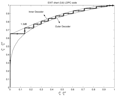
Figure 1: EXIT curves of the two component codes corresponding to the (3,6) LDPC code transmitted over an AWGN channel with $E_{b}/N_{0}=1.3$ dB

Let $I_{b}(I_{A},i)$ ($I_{c}(I_{A},i)$) be mutual information corresponding to the extrinsic output of bit (check) node of degree $i$ when the a priori mutual information is $I_{A}$. The mutual information $I$ can be calculated from the conditional distribution $f(l)$ using

$$I=\int_{-\infty}^{\infty}f(l)\log_{2}\frac{2f(l)}{f(l)+f(-l)}\ dl.$$ (5)

The EXIT curve of the bit nodes and the check nodes is given by $I_{b}=\sum\lambda_{i}I_{b}(I_{A},i)$ and $I_{c}=\sum\rho_{i}I_{c}(I_{A},i)$ respectively. Usually both $I_{b}$ and $I_{c}$ are increasing function of $I_{A}$. The convergence condition, based on the assumption on the message density, states that the EXIT curve of the bit nodes should lie above that of the check nodes for the iterative decoder to converge to the correct codeword, i.e., $I_{b}(I_{A})>I_{c}^{-1}(I_{A})$ or equivalently $I_{b}^{-1}(I_{A})<I_{c}(I_{A})$ for all $I_{A}$ where $I_{c}(I_{c}^{-1}(I_{A}))=I_{A}$. For a fixed $\rho(x)$, the problem of code design can then be stated as the following linear program

$$\max \sum\lambda_{i}/i$$

subject to: $$\sum\lambda_{i}=1,\lambda_{i}\geq 0,$$

$$\sum\lambda_{i}I_{b}(I_{A},i)>I_{c}^{-1}(I_{A})\ \ \forall I_{A}\in[0,1).$$ (6)

Note that maximizing the objective function corresponds to maximizing the rate. A similar linear program can be written for optimizing $\rho(x)$ for a given $\lambda(x)$.

IV-B Fixed Channel

We consider the problem of finding LDPC codes for a given BMS channel such that reliable communication is possible with the MS decoding algorithm. We are interested here in the performance when the block length goes to infinity. Our goal is to maximize the rate of transmission. Towards achieving this goal we first pick an LDPC code such that it converges to error free density for the specified channel.

Starting from the initial ensemble, the LDPC code ensemble is optimized in several steps. In each step, the basic idea is to design the codes using EXIT charts. However, instead of using the Gaussian assumption on the input densities, the input density in a particular step of the optimization process is assumed to be the same as the density obtained by using the density evolution procedure for the ensemble obtained in the previous step. The inherent assumption is that the input densities do not change much in one step of the optimization procedure and therefore the approximate EXIT curves obtained using the previous densities are close to the actual EXIT curves. Note that this assumption is different from the assumption that the density at iteration $i$ for a particular optimization step is same as the density at iteration $i$ in the next optimization step. If we denote the densities at iteration $i$ by $\mathsf{a}_{i}$ and consider a family of densities that includes $\{\gamma\mathsf{a}_{i}+(1-\gamma)\mathsf{a}_{i+1},\gamma\in[0,1]\}$ then the assumption made is that the family of densities does not change much in one step of the optimization. We could sample many points in this family to enforce the condition in the linear program that the EXIT curves do not intersect. However, we sample only at points $\mathsf{a}_{i}$. This is usually sufficient since if the old EXIT curves are close to each other, then we get many samples there and at other points we have more leeway so we can sample fewer times.

In each step of the optimization procedure, we generate a new dd pair from the previous dd pair in two sub-steps. In the first sub-step we change $\lambda(x)$ keeping $\rho(x)$ constant and in the next sub-step we change $\rho(x)$ while keeping $\lambda(x)$ the same. The first sub-step is as follows. We choose $\rho(x)=\rho_{old}(x)$ and optimize $\lambda(x)$ as follows. We perform density evolution with the dd pair $(\lambda_{old},\rho_{old})$ and at the end of each iteration store $I_{b}^{l}(d)$ which is the mutual information corresponding to the extrinsic output of a bit node of degree $d$ at the end of iteration $l$. The optimization then reduces to the following linear program.

$$\qquad\max\sum\lambda_{i}/i$$

$$\qquad\sum\lambda_{i}=1,\lambda_{i}\geq 0,$$

$$\qquad\sum\frac{\lambda_{i}}{i}\geq\sum\frac{\rho_{i}}{i},$$

$$\qquad\sum\lambda_{i}I_{b}^{l}(i)>\sum\lambda_{old,i}I_{b}^{l-1}(i)$$

$$\qquad\ \ +\beta\sum\lambda_{old,i}(I_{b}^{l}(i)-I_{b}^{l-1}(i))\ \ \beta\in[0,1)\ \forall l,\ \ \ \$$ (7)

$$\qquad-\delta\leq\lambda_{i}-\lambda_{old,i}\leq\delta\qquad\forall\ i,$$ (8)

$$\qquad\lambda_{2}\leq\frac{1}{B\left({\mathsf{a}_{ch}}\right)\rho^{\prime}(1)}\ \ \ \ \mbox{(from (\ref{eqn:stabCond}))}.$$ (9)

Before we explain the constraints, we note that the cost function corresponds to maximizing the rate and that the old dd pair satisfies the constraints and therefore the resulting rate is always larger than the old rate.

The Constraint (7) basically represents the condition that the EXIT curve corresponding to the bit nodes should lie above that of the check nodes. The quantity $\sum\lambda_{old,i}(I_{b}^{l}(i)-I_{b}^{l-1}(i))$ is the gap between the two EXIT curves corresponding to the old dd pair. The constant $\beta$ determines how much change in the gap is allowed. If $\beta$ is chosen to be 0 the gap between the curves can become zero while if $\beta$ is chosen to be one the gap is kept the same.

By choosing a smaller $\beta$ we weaken the constraints and therefore get a larger rate. However, since the dd pair changes, the input densities also change and therefore the actual EXIT curves change. Since the gap between the approximate EXIT curves (one obtained using the previous densities) is smaller with smaller $\beta$, the chances of the actual EXIT curves intersecting increases. We choose some value of $\beta$, perform the density evolution with the new dd pair and check if it converges. If it does, we accept the new ensemble and go to the second sub-step. If it does not converge, we increase $\beta$ and repeat this sub-step.

The Constraint (8) is introduced so that the degree distributions do not change much in an iteration which in turn will ensure that the input densities and the resulting EXIT curves do not change significantly.

The Constraint (9) is the stability condition. For the modified MS algorithm with $\alpha>1$, we replace the stability condition by the condition $\lambda_{2}\rho^{\prime}(1)<1$.

In the second sub-step we perform the density evolution with the dd pair obtained in the previous sub-step and store $I_{c}^{l}(d)$ which is the mutual information corresponding to the extrinsic output of a degree $d$ check node at the end of iteration $l$. A linear program, similar to that discussed before, can then be used to optimize the rate. As mentioned before, the rate keeps increasing with each step of the optimization process. We stop the optimization when the increase in rate becomes insignificant.

The linear program discussed above can be easily modified for the case when we have a fixed rate and we want to find a code with better threshold. This optimization procedure is available on-line at [5].

V Optimization Results

We used the optimization procedure discussed in this paper to design LDPC codes for MS. For fixed rate optimization scheme the gap to capacity varied significantly depending on the average right degree chosen. For the fixed channel optimization procedure, the final gap to capacity depended on the initial profile with which the optimization procedure was started however the variations were observed to be lesser than that in fixed rate optimization.

In Fig. 2 we show the gap to capacity and the average right degree corresponding to LDPC codes optimized for MS decoding and modified MS decoding with $\alpha=1.25$. The fixed channel optimization procedure was used to obtain these points. We observe that the gap decreases as the rate increases but it is still quite far from the Shannon capacity limit.

Comparison of the threshold of LDPC codes designed for BP but used with MS and the threshold of codes designed for MS shows that significant gains are obtained by using codes specifically designed for MS. For example, the best rate 0.5 code designed for BP from [4] has a threshold of 1.91 dB with MS which is 0.97 dB worse than the best threshold we obtained for LDPC codes that were optimized for MS [5].

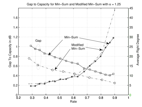
Figure 2: Gap to capacity of some optimized profiles

VI Conclusion

We derived a sufficient condition for the stability of the fixed point $\delta_{\infty}(l)$ which is also a necessary condition for the density evolution to converge to $\delta_{\infty}(l)$ when initiated with channel log-likelihood ratio density. It remains an open question whether this condition is also necessary for the stability of fixed point $\delta_{\infty}(l)$ subjected to local perturbation.

We have discussed some properties of densities which are observed to be empirically true. We proved that these properties remain preserved on the check node side. It remains to be seen if the same thing can be proved for the variable node side.

We presented a simple procedure to optimize LDPC codes for MS decoding. To the best of our knowledge, the obtained codes are the best codes reported so far for MS decoding and they perform significantly better than codes that were designed for BP but are decoded using MS. However, their performance is quite far from the capacity limit and it remains to be seen if the gap is due to the sub-optimality of the design procedure. On the other hand if the gap is due to the inherent sub-optimality of MS, it will be an interesting research direction to explain the gap by information theoretic reasoning.

Lemma 3

Let $\mathsf{a}$ and $\mathsf{b}$ be two densities and $\mathsf{c}=\mathsf{a}\boxtimes\mathsf{b}$. Then

$$B\left({\mathsf{c}}\right)\leq B\left({\mathsf{a}}\right)+B\left({\mathsf{b}}\right).$$

Proof:

For the sake of simplicity, in the proof we assume that densities $\mathsf{a}$ and $\mathsf{b}$ are absolutely continuous. However the proof also works in the general case. Let $X$ and $Y$ be two random variables with densities $\mathsf{a}$ and $\mathsf{b}$ respectively and $Z=\mathrm{sign}\left({X}\right)\mathrm{sign}\left({Y}\right)\min\left({|X|,|Y|}\right)$. Then $B\left({\mathsf{c}}\right)=\mathbb{E}\left[{e^{-\frac{Z}{2}}}\right]$,

$$B\left({\mathsf{c}}\right) = \int_{-\infty}^{\infty}\int_{-\infty}^{\infty}e^{-\frac{\mathrm{sign}\left({x}\right)\mathrm{sign}\left({y}\right)\min\left({|x|,|y|}\right)}{2}}\mathsf{a}(x)\mathsf{b}(y)dydx,$$

$$= \int_{0}^{\infty}\int_{0}^{\infty}\left({\mathsf{a}(x)\mathsf{b}(y)+\mathsf{a}(-x)\mathsf{b}(-y)}\right)e^{-\frac{\min(x,y)}{2}}dydx+$$

$$\int_{0}^{\infty}\int_{0}^{\infty}\left({\mathsf{a}(x)\mathsf{b}(-y)+\mathsf{a}(-x)\mathsf{b}(y)}\right)e^{\frac{\min(x,y)}{2}}dydx,$$

$$\stackrel{{\scriptstyle(a)}}{{=}} \int_{0}^{\infty}\int_{0}^{x}\frac{g(x,y)}{g(x,y)}\left\{\left({\mathsf{a}(x)\mathsf{b}(y)+\mathsf{a}(-x)\mathsf{b}(-y)}\right)e^{-\frac{y}{2}}\right.$$

$$\left.+\left({\mathsf{a}(x)\mathsf{b}(-y)+\mathsf{a}(-x)\mathsf{b}(y)}\right)e^{\frac{y}{2}}\right\}dydx+$$

$$\int_{0}^{\infty}\int_{x}^{\infty}\frac{g(x,y)}{g(x,y)}\left\{\left({\mathsf{a}(x)\mathsf{b}(y)+\mathsf{a}(-x)\mathsf{b}(-y)}\right)e^{-\frac{x}{2}}\right.$$ (10)

$$\left.+\left({\mathsf{a}(x)\mathsf{b}(-y)+\mathsf{a}(-x)\mathsf{b}(y)}\right)e^{\frac{x}{2}}\right\}dydx+$$

$$= I_{1}+I_{2}.$$

In $(a)$ we multiply and divide by $g(x,y)=(\mathsf{a}(x)+\mathsf{a}(-x))(\mathsf{b}(y)+\mathsf{b}(-y))$. Note that all the densities which arise in density evolution satisfy the property that $\mathsf{a}(x)=0$ if and only if $\mathsf{a}(-x)$ is zero. Thus if $\mathsf{a}(x)$ or $\mathsf{b}(y)$ are equal to zero then the integrand itself is zero and those values of $x$ and $y$ do not contribute to the integral. Hence without lose of generality we can assume that $a(x)$ and $b(y)$ are not zero. Now,

$$B\left({\mathsf{a}}\right) = \int_{0}^{\infty}\left({\mathsf{a}(x)e^{-\frac{x}{2}}+\mathsf{a}(-x)e^{\frac{x}{2}}}\right)dx,$$ (11)

$$\stackrel{{\scriptstyle(a)}}{{=}} \int_{0}^{\infty}\int_{0}^{\infty}(\mathsf{b}(y)+\mathsf{b}(-y))\left({\mathsf{a}(x)e^{-\frac{x}{2}}+\mathsf{a}(-x)e^{\frac{x}{2}}}\right)dydx,$$

$$\stackrel{{\scriptstyle(b)}}{{=}} \int_{0}^{\infty}\int_{0}^{x}\frac{(\mathsf{a}(x)+\mathsf{a}(-x))}{(\mathsf{a}(x)+\mathsf{a}(-x))}(\mathsf{b}(y)+\mathsf{b}(-y))$$

$$\left({\mathsf{a}(x)e^{-\frac{x}{2}}+\mathsf{a}(-x)e^{\frac{x}{2}}}\right)dydx+$$

$$\int_{0}^{\infty}\int_{x}^{\infty}\frac{(\mathsf{a}(x)+\mathsf{a}(-x))}{(\mathsf{a}(x)+\mathsf{a}(-x))}(\mathsf{b}(y)+\mathsf{b}(-y))$$

$$\left({\mathsf{a}(x)e^{-\frac{x}{2}}+\mathsf{a}(-x)e^{\frac{x}{2}}}\right)dydx.$$

$$= I_{\mathsf{a}1}+I_{\mathsf{a}2}.$$

In $(a)$ we used the fact that $\int_{0}^{\infty}\left({b(y)+b(-y)}\right)dy=1$ and in $(b)$ we multiply and divide by $(a(x)+a(-x))$. Similarly,

$$B\left({\mathsf{b}}\right) = \int_{0}^{\infty}\int_{0}^{x}\frac{\left({\mathsf{b}(y)+\mathsf{b}(-y)}\right)}{\left({\mathsf{b}(y)+\mathsf{b}(-y)}\right)}(\mathsf{a}(x)+\mathsf{a}(-x))$$ (12)

$$\left({\mathsf{b}(y)e^{-\frac{y}{2}}+\mathsf{b}(-y)e^{\frac{y}{2}}}\right)dydx+$$

$$\int_{0}^{\infty}\int_{x}^{\infty}\frac{\left({\mathsf{b}(y)+\mathsf{b}(-y)}\right)}{\left({\mathsf{b}(y)+\mathsf{b}(-y)}\right)}(\mathsf{a}(x)+\mathsf{a}(-x))$$

$$\left({\mathsf{b}(y)e^{-\frac{y}{2}}+\mathsf{b}(-y)e^{\frac{y}{2}}}\right)dydx.$$

$$= I_{\mathsf{b}1}+I_{\mathsf{b}2}.$$

Note that by Eqn(10, 11, 12), $B\left({\mathsf{c}}\right)-B\left({\mathsf{a}}\right)-B\left({\mathsf{b}}\right)=I_{1}-I_{\mathsf{a}1}-I_{\mathsf{b}1}+I_{2}-I_{\mathsf{a}2}-I_{\mathsf{b}2}$. We first consider $I_{1}-I_{\mathsf{a}1}-I_{\mathsf{b}1}$. We prove that the integrand of $I_{1}-I_{\mathsf{a}1}-I_{\mathsf{b}1}$ is pointwise non positive. As $(\mathsf{a}(x)+\mathsf{a}(-x))(\mathsf{b}(x)+\mathsf{b}(-x))$ is a common non negative factor in the integrands of $I_{1},I_{\mathsf{a}1}$ and $I_{\mathsf{b}1}$, we will not consider it. Then the remaining integrand of $I_{1}-I_{\mathsf{a}1}-I_{\mathsf{b}1}$ is:

$$\frac{\mathsf{a}(x)\mathsf{b}(y)e^{-\frac{y}{2}}+\mathsf{a}(x)\mathsf{b}(-y)e^{\frac{y}{2}}+\mathsf{a}(-x)\mathsf{b}(y)e^{\frac{y}{2}}+\mathsf{a}(-x)\mathsf{b}(-y)e^{-\frac{y}{2}}}{(\mathsf{a}(x)+\mathsf{a}(-x))(\mathsf{b}(y)+\mathsf{b}(-y))}\\ -\frac{\mathsf{a}(x)e^{-\frac{x}{2}}+\mathsf{a}(-x)e^{\frac{x}{2}}}{\mathsf{a}(x)+\mathsf{a}(-x)}-\frac{\mathsf{b}(y)e^{-\frac{y}{2}}+\mathsf{b}(-y)e^{\frac{y}{2}}}{\mathsf{b}(y)+\mathsf{b}(-y)}.$$ (13)

Define $q=\frac{\mathsf{b}(-y)}{\mathsf{b}(y)+\mathsf{b}(-y)}$, $p=\frac{\mathsf{a}(-x)}{\mathsf{a}(x)+\mathsf{a}(-x)}$. Now we can write Eqn (13) as

$$((1-p)(1-q)+pq)e^{-\frac{y}{2}}+(p(1-q)+q(1-p))e^{\frac{y}{2}}$$

$$-(1-q)e^{-\frac{y}{2}}-qe^{\frac{y}{2}}-(1-p)e^{-\frac{x}{2}}-pe^{\frac{x}{2}}$$

$$=p(1-2q)\left({e^{\frac{y}{2}}-e^{-\frac{y}{2}}}\right)-pe^{\frac{x}{2}}-(1-p)e^{-\frac{x}{2}}.$$ (14)

The Eqn(14) is exactly the Eqn(15) in Lemma 4 which is proved to be non positive. Also note that as required by Lemma 4, $y\leq x$ and $y$ is associated with $q$. The integrand of $I_{2}-I_{\mathsf{a}2}-I_{\mathsf{b}2}$ can also be reduced to Eqn(15) in Lemma 4. Hence we prove that $B\left({\mathsf{c}}\right)\leq B\left({\mathsf{a}}\right)+B\left({\mathsf{b}}\right)$. ∎

We define a Generalized BSC density by,

$$\mathsf{a}_{\tiny\mathrm{gbsc}(p,x)}(z)=p\delta_{-x}(z)+(1-p)\delta_{x}(z).$$

Lemma 4

Consider $\mathsf{a}_{\mathrm{gbsc}(p,x)}(z)$, $\mathsf{a}_{\mathrm{gbsc}(q,y)}(z)$ and $\mathsf{c}(z)=\mathsf{a}_{\mathrm{gbsc}(p,x)}(z)\boxtimes\mathsf{a}_{\mathrm{gbsc}(q,y)}(z)$. Then

$$B\left({\mathsf{c}}\right)-B\left({\mathsf{a}_{\mathrm{gbsc}(p,x)}}\right)-B\left({\mathsf{b}_{\mathrm{gbsc}(q,y)}}\right)\leq 0.$$

Proof:

With out loss of generality we can assume that $y\leq x$. Then

$$\mathsf{c}(z)=(p(1-q)+q(1-p))\delta_{-y}(z)+(pq+(1-p)(1-q))\delta_{y}(z).$$

Now,

$$B\left({\mathsf{c}}\right)-B\left({\mathsf{a}_{\mathrm{gbsc}(p,x)}}\right)-B\left({\mathsf{b}_{\mathrm{gbsc}(q,y)}}\right)=$$

$$(p(1-q)+q(1-p))e^{\frac{y}{2}}+(pq+(1-p)(1-q))e^{-\frac{y}{2}}$$

$$-pe^{\frac{x}{2}}-(1-p)e^{-\frac{x}{2}}-qe^{\frac{y}{2}}-(1-q)e^{-\frac{y}{2}}.$$

$$=p(1-2q)\left({e^{\frac{y}{2}}-e^{-\frac{y}{2}}}\right)-pe^{\frac{x}{2}}-(1-p)e^{-\frac{x}{2}},$$

$$\leq 0,\hskip 159.3356pt\quad$$ (15)

because $1-2q\leq 1$ and $y\leq x$, we have $p(1-2q)\left({e^{\frac{y}{2}}-e^{-\frac{y}{2}}}\right)-pe^{\frac{x}{2}}\leq 0$. Thus we have prove the desired statement. ∎

References

- [1] N. Wiberg, “Codes and Decoding on General Graphs,” PhD thesis, Linkoping University, Sweden, 1996.
- [2] R. Jotter and P. O. Vontobel, “Graph-covers and iterative decoding of finite length codes,” in Proc. 3rd International Symposium on Turbo Codes, September 2003.
- [3] A. Amraoui, “Asymptotic and finite-length optimization of LDPC codes,” Ph.d. Thesis, EPFL, June 2006.
- [4] A. Amraoui and R. L. Urbanke, LPDCopt, available at http://lthcwww.epfl.ch/research/ldpcopt/
- [5] K. Bhattad and R. L. Urbanke, LPDCopt for Min-Sum, available at http://lthcwww.epfl.ch/research/bhattad/
- [6] K. Bhattad and K. R. Narayanan, “An MSE based transfer chart to analyze and design iterative decoding schemes under the Gaussian assumption”, to appear in IEEE Trans. on Inf. Theory.
- [7] J. Chen and M. Fossorier, “Near optimum universal belief propagation based decoding of low-density parity-check codes,” IEEE Trans. Commun., vol. 50, pp. 406414, Mar. 2002.
- [8] S. ten Brink, “Convergence behaviour of iteratively decoded parallel concatenated codes,” IEEE Trans. Commun., vol. 49, pp. 1727- 1737, Oct 2001.
- [9] T. J. Richardson and R. L. Urbanke, “The capacity of low-density parity-check codes under message passing decoding,” IEEE Trans. Inf. Theory, vol. 47, no. 2, pp. 599-618, Feb. 2001.
- [10] T. Richardson, A. Shokrollahi, and R. Urbanke, “Design of capacity approaching irregular low-density parity-check codes”, IEEE Trans. Inf. Theory, vol. 47, no. 2, pp. 619-637, Feb. 2001.
- [11] A. Anastasopoulos, “A comparison between the sum-product and the min-sum iterative detection algorithms based on density evolution,” in Proc. Globecom 2001, San Antonio, TX, Nov. 2001.
- [12] J. Feldman, D. R. Karger, and M. J. Wainwright, “Using linear programming to decode linear codes,” in Proc. 37th annual Conference on Information Sciences and Systems (CISS ’03), Baltimore, MD, Mar. 12-14 2003.
- [13] P.O. Vontobel and R. Koetter, “On the relationship between linear programming decoding and min-sum algorithm decoding,” in Proc. ISITA 2004, Parma, Italy, pp. 991-996, Oct. 10-13, 2004.