Abstract

We prove a global existence theorem for the $3\times 3$ system of relativistic Euler equations in one spacial dimension. It is shown that in the ultra-relativistic limit, there is a family of equations of state that satisfy the second law of thermodynamics for which solutions exist globally. With this limit and equation of state, which includes equations of state for both an ideal gas and one dominated by radiation, the relativistic Euler equations can be analyzed by a Nishida-type method leading to a large data existence theorem, including the entropy and particle number evolution, using a Glimm scheme. Our analysis uses the fact that the equations of state are of the form $p=p(n,S)$, but whose form simplifies to $p=a^{2}\rho$ when viewed as a function of $\rho$ alone.

Chapter 1 Introduction

1.1. The Compressible Euler Equations

The compressible Euler equations form a nonlinear system of first order partial differential equations that models a gas as a continuous medium. Nearly seventy years after Newton wrote down the laws of motion in his Principia for a system of discrete particles, $\textbf{F}=m\textbf{a}$, Euler and d’Alembert produced a linear, continuum theory of sound waves. These sound waves obeyed the linear wave equation,

$$\square u=u_{tt}-c^{2}Div(u)=0,$$

where $c>0$ is the sound speed. Several years later, Euler wrote down the evolution equations for the nonlinear theory of sound waves. Today these equations are written as

$$\rho_{t}+Div\left[\rho u\right]=0,$$

$$(\rho u)_{t}+Div\left[\rho u\otimes u+pI\right]=0,$$

(1.1) $$E_{t}+Div\left[(E+p)u\right]=0,$$

where subscripts in the independent variables denotes partial differentiation and $Div=\partial/\partial x+\partial/\partial y+\partial/\partial z$. In three spacial dimensions, the compressible Euler equations (1.1), also called Euler’s equations, form a system of five equations with six unknowns, $\rho$, $\epsilon$, $u^{i}$, and $p$, which closes when an equation of state, $p=p(\rho,S)$, is prescribed. In the following we will focus our study on the case of one spacial dimension. Under this assumption, the Euler equations reduce to a system of three equations:

$$\rho_{t}+\left[\rho u\right]_{x}=0,$$

$$(\rho u)_{t}+\left[\rho u^{2}+p\right]_{x}=0,$$

(1.2) $$E_{t}+\left[(E+p)u\right]_{x}=0.$$

It is well known that even for smooth initial data, discontinuities form in the fluid variables in the solution to the Cauchy problem in finite time, [3]. Qualitatively, the nonlinearities in the equations cause waves to propagate at different speeds leading to the “breaking” of waves. See Figure 1.1. This loss of regularity corresponds to the emergence of shock waves.

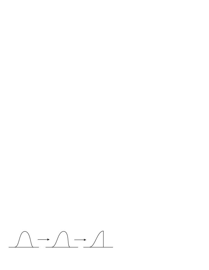
Figure 1.1. The “breaking” of a wave front which produces a shock wave.

The Euler equations are a particular example of a system of conservation laws. A system of conservation laws in one spacial dimension is a first order quasi-linear system of partial differential equations of the form

(1.3) $$U_{t}+F(U)_{x}=0,$$

where $U=(U_{1},\ldots,U_{n})$ are the conserved quantities and $F(U)=(F_{1}(U),\ldots,F_{n}(U))$ the fluxes. Much of the early work on the general structure of systems of conservation laws was set out by Lax, [5]. Lax’s results provided the foundation necessary for Glimm to give the first general existence theorem in $1965$, [4]. Glimm’s fundamental result provided a new way to analyze shock wave interactions. In the $1990$’s, Bressan, Liu and Yang headed a push for the well posedness of the general $n\times n$ Cauchy problem, [2].

A Nishida system is a specific class of conservation laws, which in certain cases includes the the Euler and Relativistic Euler equations, that allows one to prove global existence of solutions. In particular, the shock-rarefaction curves in a Nishida system behave nicely in the large. Nishida and Smoller were first to gave a global, large initial data, existence proof for the compressible Euler equations with a particular equation of state, [8]. Shortly after this, Temple extended Nishida and Smoller’s global existence result by including the entropy evolution of the gas, [12]. More recently, Smoller and Temple proved that under certain conditions the Relativistic Euler equations also form a Nishida system, [10].

It should be noted that the existence theorem for a general system of conservation laws comes at a cost; we require the initial data to be of sufficiently small total variation. The smallness requirement is needed because the structure of the shock-rarefaction curves can exhibit complicated nonlinear phenomenon in the large. When sufficiently small data is considered, the analysis can be confined within a small region in state space in which the shock-rarefaction curves have a canonical structure that can be exploited when analyzing solutions.

1.2. The Relativistic Euler Equations

In $1905$, Einstein introduced the special theory of relativity. Within this framework one can generalize the classical Euler equations to obtain equations that fit within the theory of relativity.

The relativistic compressible Euler equations in one spatial dimension form a system of three equations,

$$(u^{\alpha}n),_{\alpha} = 0,$$

(1.4) $$T^{\alpha\beta},_{\alpha} = 0,\phantom{44}\beta=0,1,$$

where $T^{\alpha\beta}$ is the stress energy tensor for a perfect fluid,

$$T^{\alpha\beta}=(\rho+p)u^{\alpha}u^{\beta}+p\eta^{\alpha\beta},$$

and the subscript “$,\alpha$” denotes partial differentiation with respect to the coordinate $x^{\alpha}$. We will use Einstein’s summation convention where repeated up-down indices are summed and adopt the following notation:

$$u^{\alpha} \textrm{Components of the }2\textrm{-Velocity}$$

$$\rho$$ Proper Rest Energy Density

$$p$$ Pressure

$$\epsilon$$ Specific Internal Energy

$$n$$ Baryon Number

$$S$$ Specific Entropy

$$T$$ Temperature

The components of the Minkowski metric $\eta^{\alpha\beta}$ are given by

$$\eta^{\alpha\beta}=\left(\begin{array}[]{rc}-1&0\\ 0&1\\ \end{array}\right).$$

For convenience, we will also use units where the speed of light is unit, $c=1$. The proper energy density, $\rho$, is related to the particle number density and the internal energy by $\rho=n(1+\epsilon)$, [14]. This equation is the sum of the rest mass energy $nc^{2}=n$ and the internal energy $n\epsilon$. Furthermore, thermodynamics provides a functional relationship between the quantities, $\epsilon$, $T$, $S$, $p$ and $n$. This relationship is given by the second law of thermodynamics, [3]:

(1.5) $$d\epsilon=TdS+\frac{p}{n^{2}}dn.$$

The relativistic Euler equations (1.2) can be written as a system of conservation laws by choosing a particular Lorentz frame and writing the instantaneous worldline trajectory of the fluid, $u^{\alpha}$, in terms of the classical velocity $v$. The components of $(u^{0},u^{1})$ are proportional to the vector $(1,v)$ and is of unit length according to the inner-product defined by the metric $\eta$. From this we find the components $u^{\alpha}$ are related to $v$ by

$$\left(u^{0},u^{1}\right)=\left(\frac{1}{\sqrt{1-v^{2}}},\frac{v}{\sqrt{1-v^{2}}}\right).$$

Using this, the first equation is equivalent to

$$\frac{\partial}{\partial{t}}\left(\frac{n}{\sqrt{1-v^{2}}}\right)+\frac{\partial}{\partial x}\left(\frac{nv}{\sqrt{1-v^{2}}}\right)=0.$$

The second and third equations in (1.2) can also be rewritten. With $\beta=0$ we find $T^{0\alpha}_{\phantom{00},\alpha}=0$ gives

$$\frac{\partial}{\partial t}\left((\rho+p)\frac{1}{1-v^{2}}-p\right)+\frac{\partial}{\partial x}\left((\rho+p)\frac{v}{1-v^{2}}\right)=0$$

and with $\beta=1$, $T^{1\alpha}_{\phantom{00},\alpha}=0$ gives

$$\frac{\partial}{\partial t}\left((\rho+p)\frac{v}{1-v^{2}}\right)+\frac{\partial}{\partial x}\left((\rho+p)\frac{v^{2}}{1-v^{2}}+p\right)=0.$$

Simplifying the terms inside, we can write the system (1.2) as the system of conservation laws,

(1.6) $$U_{t}+F(U)_{x}=0,$$

where,

(1.7) $$U=\left(\frac{n}{\sqrt{1-v^{2}}}\phantom{3}\!,\left(\rho+p\right)\frac{v}{1-v^{2}}\phantom{3}\!,\left(\rho+p\right)\frac{v^{2}}{1-v^{2}}+\rho\right)$$

and

(1.8) $$F(U)=\left(\frac{nv}{\sqrt{1-v^{2}}}\phantom{3}\!,\left(\rho+p\right)\frac{v^{2}}{1-v^{2}}+p\phantom{3}\!,\left(\rho+p\right)\frac{v}{1-v^{2}}\right).$$

It is interesting to note that the relativistic Euler equations are indeed a generalization of the classical Newtonian equations of hydrodynamics (1.1). To see this we view (1.6) under the assumptions of a classical fluid; fluid velocities are small compared to the speed of light and the pressure is dominated by the rest mass. More specifically, we assume $|v|\ll 1$ and $p/\rho\ll 1$. Under these assumptions the equations $T^{\alpha\beta}_{\phantom{33},\alpha}=0$ become the equations of motion of a classical gas:

$$\frac{\partial}{\partial t}\rho+\frac{\partial}{\partial x}(\rho v)=0$$

and

$$\frac{\partial}{\partial t}(\rho v)+\frac{\partial}{\partial x}(\rho v^{2}+p)=0.$$

Notice that the density of the fluid in the classical Euler equations is now replaced by the proper mass-energy density. The new variable $n$ is used for conservation of particle number.

Nearly all terrestrial phenomenon falls into the classical, Newtonian case. In a hurricane, for example, wind speeds may reach speeds of $90m/s$. However, this velocity is insignificant when compared to the speed of light,

$$|v|\sim 90m/s\sim 3\times 10^{-7}c=10^{-7}\ll 1.$$

Furthermore, the pressure to mass density ratio, $p/\rho$, can be shown to be of the order of $10^{-12}$, [7]. In this situation the classical Euler equations would certainly suffice.

It is clear from the last example that even in seemingly extreme situations on Earth, they are far from relativistic events. We must look to the cosmos to find examples where a gas has a high enough pressure to make $p/\rho$ non-negligible and sufficiently high velocity to make the relativistic correction terms such as $1/\sqrt{1-v^{2}}$ important to the gas’ evolution. These situations arise in astrophysical events such as gamma-ray bursts, solar flares and in remnants of supernovas. The relativistic Euler equations are also used in modeling the early universe, [13].

Like the classical Euler equations, the relativistic Euler equations are not closed; an equation of state relating thermodynamic variables is needed to close the system. This choice of equation of state changes the characteristics of the evolution of the gas and has a significant effect on the complexity of its analysis. A natural equation of state for a gas is one satisfying the ideal gas law and whose internal energy is proportional to its temperature. Using the second law of thermodynamics, one finds the relation

(1.9) $$\epsilon(n,S)=e^{\frac{\gamma-1}{R}S}n^{\gamma-1},$$

which for some constant $\gamma>1$ is called a polytropic equation of state. A polytropic equation of state is typically used to model air in the classical sense with $\gamma\approx 1.4$. It is known that using this equation of state vacuums may form in a solution to (1.1) and (1.2) when velocities and densities are sufficiently large to completely void a region of matter. Vacuums pose problems in the standard estimating techniques and at this point prevents one from obtaining large data existence theorems, [9].

A class of equations of state one typically encounters which still include most desirable dynamics are called barotropic, given by $p=p(\rho)$. The class of equations of state, $p=a^{2}\rho^{\gamma}$, for $1<\gamma<2$ are barotropic and are used in astrophysical modeling. In this case $0<a$ is constant, [1].

If one considers (1.10), the limiting case of the barotropic equation of state $p=a^{2}\rho^{\gamma}$ when $\gamma=1$, the system (1.6) contains special properties; in this limit one can prove global solutions exist for initial data with arbitrarily large, but finite, total variation, [10]. Moreover, vacuums do not form in the solution.

(1.10) $$p=a^{2}\rho$$

In this thesis we will extend these results to prove large data existence theorem for an ultra-relativistic gas with an equation of states of the form

(1.11) $$\epsilon(n,S)=A(S)n^{\gamma-1},$$

where the function $A$ satisfies the following conditions:

(A1) $$A:\mathbb{R}^{+}\rightarrow\mathbb{R}^{+},$$

(A2) $$A\in\mathcal{C}^{1}(\mathbb{R}^{+}),$$

(A3) $$A^{\prime}(S)>0\phantom{3}\mathrm{for}\phantom{3}S>0.$$

The family (1.11) includes equations of state for a polytropic gas (1.9) and one dominated by radiation satisfying

(1.12) $$\epsilon(n,S)=\frac{a_{R}T^{\frac{\gamma}{\gamma-1}}}{n}.$$

Using the relation $\rho=n(1+\epsilon)$, the equations of state (1.11) do not reduce to (1.10). However, they do in the ultra-relativistic limit. For the ultra-relativistic limit, we assume the internal energy dominates the rest mass energy; in other words, $\rho=n\epsilon$. Under this assumption, an equation of state of the form (1.11) reduces to an equation of state of the form (1.10) with $a^{2}=(\gamma-1)$. We take advantage of the fact that in this limit the pressure is still a function of $n$ and $S$, but whose form reduces to (1.10) when viewed as a function of $\rho$ alone. This model now allows one to find the entropy and particle number density evolution of the gas and still take advantage of the simplifying effects of an equation of state of the form (1.10).

The particular equation of state (1.12) is also used to model massless thermal radiation. In this case the ultra-relativistic assumption is not needed since the mass-energy in $\rho$ drops out, leaving only the internal energy. In particular for $\gamma=4/3$, the radiation dominated equation of state is used to model the early universe, because this radiation has been predicted to make the dominant energy contribution, [13]. In either situation, massless particles or in the ultra-relativistic limit, we still have an equation of state of the form (1.10).

It is interesting that for the classical Euler equations there is only one way to assign an entropy profile to a gas with an equation of state of the form (1.10). This equation of state is given by

(1.13) $$\epsilon(\rho,S)=a^{2}\ln\left(\rho\right)+\frac{a^{2}S}{R}+C,$$

for constants $a>0$, $C>0$. A global existence theorem for the classical Euler equations with this equation of state was given by Temple in [12].

1.3. Statement of Main Theorem

The goal of this paper is to prove the following:

1 Theorem.

Let $\rho_{0}(x)$, $v_{0}(x)$ and $S_{0}(x)$ be arbitrary initial data satisfying, $\rho_{0}(x)>0$, $-1<v_{0}(x)<1$ and $S_{0}(x)>0$. Let $\Sigma=\ln\left[A(S)\right]$ for $\epsilon(n,S)=A(S)n^{\gamma-1}$, $1<\gamma<2$, and $A$ satisfying (A1), (A2) and (A3). Suppose further that

(1.14) $$Var\{\Sigma_{0}(\cdot)\}<\infty,$$

(1.15) $$Var\{\ln(\rho_{0}(\cdot))\}<\infty,$$

and

(1.16) $$Var\Bigg{\{}\ln\left(\frac{1+v_{0}(\cdot)}{1-v_{0}(\cdot)}\right)\Bigg{\}}<\infty.$$

Then there exists a bounded weak solution $\{\rho(x,t),v(x,t),S(x,t)\}$ to (1.6) in the Ultra-Relativistic limit, satisfying

(1.17) $$Var\{\Sigma(\cdot,t)\}<N,$$

(1.18) $$Var\{\ln(\rho(\cdot,t))\}<N,$$

and

(1.19) $$Var\Bigg{\{}\ln\left(\frac{1+v(\cdot,t)}{1-v(\cdot,t)}\right)\Bigg{\}}<N,$$

where $N$ is a constant depending only on the initial variation bounds in (1.14), (1.15), and (1.16).

It should be noted that Theorem 1 is a generalization of the work by Smoller and Temple in [10] that includes the entropy evolution. In other words, in this model we are able to prove global solutions exist including a physically relevant entropy and particle number density profile. Smoller and Temple found that the relativistic Euler equations with equation of state (1.10) possessed the property that after each elementary wave interaction in a Glimm scheme, $Var\{\ln(\rho)\}$ is non-increasing. This functional, introduced by Liu, is used as a replacement for the quadratic potential in Glimm’s original analysis, which can be used to show that (1.15) and (1.16) implies (1.18) and (1.19). Considering the ultra-relativistic limit, the solutions of Riemann problems are independent of the value of $S$, enabling one to solve for the intermediate state in the projected state space and place a corresponding entropy wave between them.

In [10] it is shown that for an equation of state of the form (1.10), the shock curves are translationally invariant in the plane of Riemann invariants. In our case, this property continues to hold under certain coordinate changes in the three dimensional non-projected state space for an equation of state of the form (1.11). This can be viewed as the relativistic analogue of the large data existence result in [12] with a family of distinct entropy profiles.

The main part of the analysis is showing that $Var\{S\}$ is bounded in our approximate solutions. We extend the analysis by Smoller and Temple for the ultra-relativistic regime with equation of state given by (1.11), by utilizing the geometry of the shock curves in the space of Riemann invariants. If we only considered the variation of $S$ across shock waves, we find that $Var\{S\}$ is uniformly bounded by $Var\{\ln(\rho)\}$ for a polytropic equation of state. However, across the linearly degenerate entropy waves, there is no change in pressure, and hence no jump in proper energy density by (1.10). Thus, another method must be employed to estimate the strengths of these jumps. For a gas dominated by radiation or for a general equation of state of the form (1.11), the situation seems more dire as the change in entropy across a shock depends on the initial entropy value. It is not known a priori that this dependence does not lead to blow-up in the variation in $S$.

Furthermore, in certain elementary wave interactions, $Var\{S\}$ may actually increase while $Var\{\ln(\rho)\}$ remains invariant. Complicating matters, using $\Delta\ln(\rho)$ as the definition of wave strengths increases the technicality of the entropy wave estimates. For example, after the interaction of two shocks of the same family, the entropy change across the new shock may be less than the sum of the jumps across the two preceding shock waves. This happens because the new shock wave has strength less than the sum of the two previous. In other words when two shock waves combine, the strengths are not simply additive, but the new wave strength is strictly less than the simple sum of the incoming shock strengths. It follows that under certain circumstances the change in entropy across the new single shock may be less than the sum of the entropy jumps across the approaching shocks.

To alleviate these technicalities, we propose a more classical approach by using the change of Riemann invariants as a measure of wave strength. More specifically, the strength of a $1(3)-$shock is determined by the change in the first$($third$)$-Riemann invariant and the contact discontinuity by the change in entropy or a specific change in a function of the entropy. Using the change in Riemann invariants as a measure of wave strength for a Nishida system was used to prove existence of solutions in [6], [8] and [12]. Under this regime, wave strengths are now additive and the sum of all the strengths of shock waves is shown to be non-increasing in time. Moreover, the wave interaction estimates can be analyzed as in the classical case. In conclusion, using $\Delta\ln(\rho)$ as a measure of wave strength dramatically simplifies the interaction estimates for the nonlinear waves, but complicates the problem dealing with entropy.

In summary, we show there exists a family of equations of state, which include the case of a polytropic and radiation dominated gas, that one can use and obtain a global existence theorem. These equations of state allow one to also calculate the entropy and particle density associated with the gas. This is in contrast with the classical case where there is one equation of state with the same properties corresponding to very heavy molecules.

The rest of this paper is outlined as follows:

In Chapter 2, we give a detailed analysis of the structure of simple wave solutions of (1.6). Using these properties, we prove global existence of solutions to Riemann problems. Furthermore, we obtain a priori wave interaction estimates which will be used to produce estimates on approximate solutions constructed using a Glimm scheme in Chapter 3.

In Chapter 3 we give an overview of the Glimm difference scheme and prove estimates on the approximate solutions obtained for system (1.6). Chapter 4 contains the proof of our main theorem.

Chapter 2 Relativistic Gas Dynamics

2.1. Gas Dynamics

We consider a gas where the proper energy density and pressure satisfy the relationship (1.10). Causality restricts the sound speed $c_{s}=\sqrt{dp/d\rho}=a$ to be less than unity. Under assumption (1.10), the system (1.6) decouples so that we may solve for two variables first, then solve for the third afterward. In this section, we will show in the domain $\rho>0$, $-1<v<1$, and $S>0$, Riemann problems are globally solvable and their general structure consists of two waves separated by a jump in entropy traveling with the fluid. We then discuss wave interaction estimates which will allow us to prove global existence of solutions using a Glimm scheme in Chapter 4. Our analysis uses the special geometry of the shock and rarefaction curves in the space of Riemann invariants.

To begin, we will compute the eigenvalues and eigenvectors associated with the relativistic Euler equations (1.6). In order to simplify this process, we will exchange the first equation, conservation of particle number, with the equivalent equation that says that entropy is constant along flow lines. We note that this equation holds for continuous solutions, but fails when shock waves form since entropy increases across shocks, [3].

2.1 Proposition.

For smooth solutions of (1.6), the following supplemental equation holds:

(2.1) $$u^{\alpha}S_{,\alpha}=0.$$

More specifically after choosing a particular Lorentz frame,

(2.2) $$S_{t}+vS_{x}=0.$$

Proof.

We show that conservation of energy and momentum is equivalent to continuous flow being adiabatic, i.e. (2.2). We take the stress-energy tensor of a perfect fluid,

$$T^{\alpha\beta} = n\left(1+\epsilon+\frac{p}{n}\right)u^{\alpha}u^{\beta}+p\eta^{\alpha\beta},$$

$$= n\omega u^{\alpha}u^{\beta}+p\eta^{\alpha\beta},$$

with $\omega=\left(1+\epsilon+\frac{p}{n}\right)$ for convenience. Then conservation of energy-momentum equation, $T^{\alpha\beta}_{\phantom{\alpha\beta},\beta}=0$, is given by

(2.3) $$0 = T^{\alpha\beta}_{\phantom{\alpha\beta},\beta},$$

$$= \left(n\omega u^{\alpha}u^{\beta}\right)_{,\beta}+p_{,\beta}\eta^{\alpha\beta},$$

$$= nu^{\beta}\left(\omega u^{\alpha}\right)_{,\beta}+p_{,\beta}\eta^{\alpha\beta}.$$

where conservation of particle number, $\left(nu^{\beta}\right)_{,\beta}=0$, is used in the last step. Multiplying (2.3) by $-u_{\alpha}$ and summing we find,

(2.4) $$0=-u_{\alpha}T^{\alpha\beta}_{\phantom{\alpha\beta},\beta}=-nu^{\beta}\left(\omega u^{\alpha}\right)_{,\beta}u_{\alpha}-p_{,\beta}u^{\beta}.$$

To simplify this expression, we claim,

$$u_{\alpha}\left(\omega u^{\alpha}\right)_{,\beta}=-\omega_{,\beta}.$$

Indeed,

$$u_{\alpha}\left(\omega u^{\alpha}\right)_{,\beta}=u_{\alpha}u^{\alpha}\omega_{,\beta}+\left(u_{\alpha}u^{\alpha}_{\phantom{\alpha},\beta}\right)\omega=-\omega_{,\beta},$$

where the second term, $\left(u_{\alpha}u^{\alpha}_{\phantom{\alpha},\beta}\right)\omega$, vanishes because

$$0=\left(u_{\alpha}u^{\alpha}\right)_{,\beta}=2u_{\alpha}u^{\alpha}_{\phantom{\alpha},\beta}.$$

Thus, (2.4) now reads,

$$0 = n\omega_{,\beta}u^{\beta}-p_{,\beta}u^{\beta},$$

$$= \left(\epsilon_{,\beta}u^{\beta}+\left(\frac{p}{n}\right)_{\!\!,\beta}u^{\beta}\right)-p_{,\beta}u^{\beta},$$

$$= n\left(\epsilon_{,\beta}u^{\beta}+\left(\frac{1}{n}\right)p_{,\beta}u^{\beta}+p\left(\frac{1}{n}\right)_{\!\!,\beta}u^{\beta}\right)-p_{,\beta}u^{\beta},$$

$$= n\left(\epsilon_{,\beta}+p\left(\frac{1}{n}\right)_{\!\!,\beta}\right)u^{\beta},$$

$$= nTS_{,\beta}u^{\beta}.$$

The last step follows from the second law of thermodynamics. Since $n,T\neq 0$ we conclude, $u^{\beta}S_{,\beta}=0$. Furthermore, after choosing a particular frame of reference and replacing the worldline trajectory with

$$u=\left(\frac{1}{\sqrt{1-v^{2}}},\frac{v}{\sqrt{1-v^{2}}}\right),$$

we get

$$\frac{1}{\sqrt{1-v^{2}}}S_{t}+\frac{v}{\sqrt{1-v^{2}}}S_{x}=0.$$

In particular, since $\frac{1}{\sqrt{1-v^{2}}}\neq 0$, (2.2) holds. ∎

It is interesting to note that (2.1) continues to hold in curved spacetimes within general relativity. For this case, differentiation is replaced by covariant differentiation.

In order to solve the Riemann problem by a series of simple waves, we need to know that the corresponding wave speeds are distinct. If this is the case the system is strictly hyperbolic.

2.2 Definition.

We call a system of conservation laws (1.3) Strictly Hyperbolic in an open connected subset $U\subseteq\mathbb{R}^{n}$ if at each point $u\in U$, $dF$ has $n$ real distinct eigenvalues, $\{\lambda_{i}(u)\}_{i=1}^{n}$, such that

$$\lambda_{1}(u)<\ldots<\lambda_{n}(u).$$

Since a strictly hyperbolic system has $n$ distinct eigenvalues, the corresponding eigenvectors form a basis at every point in $U$. Along with strict hyperbolicity, we require one more assumption on the eigenvector-eigenvalue pairs; the corresponding eigenvalues are either constant or monotonically increasing or decreasing along the integral curves determined by the eigenvectors.

2.3 Definition.

Let $\left\{(\lambda_{i}(u),R_{i}(u))\right\}_{i=1}^{n}$ be the eigenvalue-eigenvector pairs associated with $dF$ for a strictly hyperbolic conservation law in an open connected subset $U\subseteq\mathbb{R}^{n}$ with $\lambda_{1}(u)<\ldots<\lambda_{n}(u)$. We call the $\textrm{i}^{\textrm{th}}$ characteristic field Genuinely Non-Linear in $U$ if for all $u\in U$,

$$R_{i}(u)\cdot\nabla\lambda_{i}(u)\neq 0,$$

and Linearly Degenerate if for all $u\in U$,

$$R_{i}(u)\cdot\nabla\lambda_{i}(u)=0.$$

In the following proposition we characterize the three eigenclasses of the system (1.6).

2.4 Proposition.

Let $p=a^{2}\rho$ with $0<a<1$. Then the system $\eqref{System-Conservation}$ is strictly hyperbolic at $(\rho,v,S)$ for $\rho>0$, $-1<v<1$ and $S>0$. Furthermore, the first and third characteristic fields are genuinely non-linear and the second linearly degenerate.

Proof.

Equivalent systems of equations possess the same eigenvalues, so we will replace the conservation of particle number equation with the equivalent equation (2.2). Since the flux functions (1.8) are complicated implicit functions of the conserved variables (1.7), our plan is to rewrite the conservation laws (1.6) as

$$\omega_{t}+G(\omega)\omega_{x}=0,$$

where $\omega=(\rho,v,S)^{T}$, then calculate the eigenvalues and eigenvectors in terms of these variables. To do this we rewrite (1.6) using the chain rule as

$$A(\omega)\omega_{t}+B(\omega)\omega_{x}=0,$$

then find $G(\omega)$ by multiplying on the left by $A^{-1}$ to get

$$\omega_{t}+\left[A^{-1}B\right](\omega)\omega_{x}=0.$$

By the chain rule,

$$A(\omega)=\left[\begin{array}[]{ccc}0&0&1\\ (a^{2}+1)\frac{v}{1-v^{2}}&(a^{2}+1)\rho\frac{1+v^{2}}{(1-v^{2})^{2}}&0\\ (a^{2}+1)\frac{v^{2}}{1-v^{2}}+1&(a^{2}+1)\rho\frac{2v}{(1-v^{2})^{2}}&0\\ \end{array}\right]$$

and

$$B(\omega)=\left[\begin{array}[]{ccc}0&0&v\\ (a^{2}+1)\frac{v^{2}}{1-v^{2}+a^{2}}&(a^{2}+1)\rho\frac{2v}{(1-v^{2})^{2}}&0\\ (a^{2}+1)\frac{v}{1-v^{2}}&(a^{2}+1)\rho\frac{1+v^{2}}{(1-v^{2})^{2}}&0\\ \end{array}\right].$$

Note that $A(\omega)$ is invertible because for $-1<v<1$ and $\rho>0$,

$$Det[A(\omega)]=\frac{(1+a^{2})(a^{2}v^{2}-1)}{(1-v^{2})^{2}}\rho\neq 0.$$

After some work we get

$$A^{-1}(\omega)=\left[\begin{array}[]{ccc}0&\frac{2v}{a^{2}v^{2}-1}&\frac{1+v^{2}}{1-a^{2}v^{2}}\\ 0&\frac{(1-v^{2})(1+a^{2}v^{2}}{(a^{2}+1)\rho(1-a^{2}v^{2})}&\frac{v^{3}-v}{\rho(1-a^{2}v^{2})}\\ 1&0&0\\ \end{array}\right].$$

Therefore,

$$G(\omega)=\left[A^{-1}B\right](\omega)=\left[\begin{array}[]{ccc}\frac{(a^{2}-1)v}{a^{2}v^{2}-1}&\frac{(a^{2}+1)\rho}{1-a^{2}v^{2}}&0\\ \frac{a^{2}(1-v^{2})^{2}}{(a^{2}+1)\rho(a^{2}v^{2}-1)}&\frac{(a^{2}-1)v}{a^{2}v^{2}-1}&0\\ 0&0&v\\ \end{array}\right].$$

We look for the roots of the characteristic polynomial,

$$0=\textrm{Det}\left[G(\omega)-\lambda I\right]=\frac{(v-\lambda)(\lambda(-1+av)-a+v)(-a-v+\lambda(1+av))}{(av-1)(1+av)}.$$

There are three values of $\lambda$ that make the numerator zero,

(2.5) $$\lambda_{1}=\frac{v-a}{1-va},\phantom{3333}\lambda_{2}=v,\phantom{3333}\lambda_{3}=\frac{v+a}{1+va}.$$

We show for $0<a<1$ and $-1<v<1$,

$$\lambda_{1}<\lambda_{2}<\lambda_{3}.$$

Indeed,

$$v^{2}<1\Longleftrightarrow-av^{2}>-a\Longleftrightarrow v-av^{2}>v-a.$$

By the restrictions on $v$ and $a$, $(1-av)>0$ and thus,

$$v(1-av)>v-a\Longleftrightarrow v>\frac{v-a}{1-av}.$$

Showing $v<(v+a)/(1+va)$ is similar, we omit the details. We conclude that for $\rho>0$, $-1<v<1$, and $S>0$ the system (1.6) is strictly hyperbolic.

Now, we show that the first and third characteristic fields are genuinely nonlinear and the second is linearly degenerate. To do this we need to find the eigenvectors of $G(\omega)$. For $\lambda_{2}$ we simply find

$$R_{2}(\rho,v,S)=(0,0,1)^{T},$$

and after some work,

$$R_{1}(\rho,v,S)=\left(-\frac{(a^{2}+1)\rho}{a(1-v^{2})},1,0\right)^{T}$$

and

$$R_{3}(\rho,v,S)=\left(\frac{(a^{2}+1)\rho}{a(1-v^{2})},1,0\right)^{T}.$$

Computing the gradients of the eigen-fields with respect to $\omega=(\rho,v,S)$,

$$\nabla\lambda_{1} = \left(0,\frac{1-a^{2}}{(1-av)^{2}},0\right),$$

$$\nabla\lambda_{2} = \left(0,1,0\right),$$

$$\nabla\lambda_{3} = \left(0,\frac{1-a^{2}}{(1+av)^{2}},0\right).$$

Thus,

$$R_{1}\cdot\nabla\lambda_{1} = \frac{1-a^{2}}{(1-av)^{2}}\neq 0,$$

$$R_{2}\cdot\nabla\lambda_{2} = 0,$$

$$R_{3}\cdot\nabla\lambda_{3} = \frac{1-a^{2}}{(1+av)^{2}}\neq 0.$$

The first and third are non-zero and bounded by the restrictions on $a$ and $v$. ∎

It is interesting to note that the eigenvalues (2.5) are the relativistic analog of the sum of the local sound speed and fluid velocity in the classical Euler equations. In the classical case, the first and third characteristic fields have eigenvalues $\lambda_{1}=u-c$ and $\lambda_{3}=u+c$, which are the sum and differences of the fluid speed and the local speed of sound respectively. The eigenvalues (2.5) are exactly the relativistic sum of two velocities within the frame work of relativity.

2.2. Riemann Invariants

The Riemann invariants for the system (1.6) can be found from the eigenvectors. An $i^{\textrm{th}}-$Riemann invariant is a function $\psi$ such that

$$R_{i}\cdot\nabla\psi=0.$$

In other words, the level curves of $\psi$ are the integral curves of the $i^{\textrm{th}}$ characteristic field. We will perform our interaction estimate analysis in the coordinate system of Riemann invariants because the rarefaction curves have particularly simple structure; straight lines parallel to the coordinate axes. From the eigenvector $R_{1}$ we see that along $1-$rarefaction curves,

$$\frac{d\rho}{dv}=-\frac{a^{2}+1}{a}\frac{\rho}{1-v^{2}},$$

which we can explicitly solve to find that along the first integral curve,

$$\frac{a}{a^{2}+1}\ln(\rho)+\frac{1}{2}\ln\left(\frac{1+v}{1-v}\right)=\textrm{const.}$$

This can be done for the third integral curve in a similar fashion. We therefore define:

$$r=\frac{1}{2}\ln\left(\frac{1+v}{1-v}\right)-\frac{a}{1+a^{2}}\ln(\rho),$$

(2.6) $$s=\frac{1}{2}\ln\left(\frac{1+v}{1-v}\right)+\frac{a}{1+a^{2}}\ln(\rho).$$

The function $r=r(\rho,v)$ is constant across $3-$rarefaction waves and $s=s(\rho,v)$ is constant across $1-$rarefaction waves. From the supplemental equation (2.2), we see that the entropy, $S$, is a third Riemann invariant constant across $1$ and $3-$rarefaction waves. In our analysis, we will view state space in the coordinates of the Riemann invariants rather than the conserved variables. However, using $S$ is not sufficient because the shock curves in $(r,s,S)$ space are, in general, not translationally invariant. Instead we will use $\Sigma=\ln(A(S))$ as our third coordinate. It will be shown in Section 2.4 that in $(r,s,\Sigma)$ space, the shock-rarefaction curves are indeed independent of base point. Since $S$ is a Riemann invariant, $\ln(A(S))$ must be one too. Indeed, suppose that $\psi$ is a $i^{\textrm{th}}-$Riemann invariant and let $f\in\mathcal{C}^{1}(\mathbb{R},\mathbb{R})$. Then $f(\psi)$ is an $i^{\textrm{th}}-$Riemann invariant as well since,

$$R_{i}\cdot\nabla f(\psi)=f^{\prime}(\psi)R_{i}\cdot\nabla\psi=0.$$

We now change our variables from the conserved quantities $(U_{1},U_{2},U_{3})$ to $(\rho,v,S)$.

2.5 Proposition.

In the region, $\rho>0$, $-1<v<1$, $S>0$, the mapping $(\rho,v,S)\to(U_{1},U_{2},U_{3})$ is one-to-one, and the Jacobian determinant of the map is both continuous and non-zero.

Proof.

We will show first that the map $(\rho,v)\rightarrow(U_{2},U_{3})$ is one-to-one for $\rho>0$ and $-1<v<1$. Assume the contrary. Suppose we have $(\rho_{1},v_{1})$ and $(\rho_{2},v_{2})$ such that $U_{2}(\rho_{1},v_{1})=U_{2}(\rho_{2},v_{2})$ and $U_{3}(\rho_{1},v_{1})=U_{3}(\rho_{2},v_{2})$. To begin we show that if $v_{1}=v_{2}=v$ then $\rho_{1}=\rho_{2}$. From the equality $U_{3}(\rho_{1},v)=U_{3}(\rho_{2},v)$ we have

$$\rho_{1}\left((a^{2}+1)\frac{v^{2}}{1-v^{2}}+1\right)=\rho_{2}\left((a^{2}+1)\frac{v^{2}}{1-v^{2}}+1\right).$$

Since the term

$$\left((a^{2}+1)\frac{v^{2}}{1-v^{2}}+1\right)\neq 0$$

for any $-1<v<1$ we must have $\rho_{1}=\rho_{2}$. We now show that if the images of $U_{2}$ and $U_{3}$ are equal, then we must have $v_{1}=v_{2}$ and, by the previous argument, $\rho_{1}=\rho_{2}$.

From $U_{3}(\rho_{1},v_{1})=U_{3}(\rho_{2},v_{2})$ and $U_{2}(\rho_{1},v_{1})=U_{2}(\rho_{2},v_{2})$ we have

(2.7) $$\frac{\rho_{1}}{\rho_{2}}\left((a^{2}+1)\frac{v_{1}^{2}}{1-v_{1}^{2}}+1\right)=\left((a^{2}+1)\frac{v_{2}^{2}}{1-v_{2}^{2}}+1\right)$$

and

$$\frac{\rho_{1}}{\rho_{2}}=\left(\frac{v_{1}}{1-v_{1}^{2}}\right)^{-1}\left(\frac{v_{2}}{1-v_{2}^{2}}\right).$$

Note that if $v_{1}/(1-v_{1}^{2})=0$ we must also have $v_{1}=0$ and by (2.7), $v_{2}=0$ since $\rho_{1}/\rho_{2}\neq 0$. Assume that $v_{1}\neq 0$.

Replacing $\rho_{1}/\rho_{2}$ in (2.7) and simplifying,

$$\frac{a^{2}v_{1}^{2}+1}{v_{1}}=\frac{a^{2}v_{2}^{2}+1}{v_{2}},$$

which further reduces to

$$(v_{1}-v_{2})(a^{2}v_{1}v_{2}-1)=0.$$

Since $|a|,|v_{1}|,|v_{2}|<1$, the second term, $(a^{2}v_{1}v_{2}-1)\neq 0$, so it must be $v_{1}=v_{2}$. Therefore, the mapping $(\rho,v)\longleftrightarrow(U_{2},U_{3})$ is one-to-one.

Now we show that the mapping $(\rho,v,S)\rightarrow(U_{1},U_{2},U_{3})$ is one-to-one. Proceed again by contradiction by supposing $(\rho_{1},v_{1},S_{1})$ and $(\rho_{2},v_{2},S_{2})$ have the same image. Since $U_{2}$ and $U_{3}$ only depend on $\rho$ and $v$, the previous argument shows that $\rho_{1}=\rho_{2}$ and $v_{1}=v_{2}$. We now show that $S_{1}=S_{2}$. Since $n=n(\rho,S)$ the equality $U_{1}(\rho_{1},v_{1},S_{1})=U_{1}(\rho_{2},v_{2},S_{2})$ reduces to

$$n(\rho,S_{1})=n(\rho,S_{2}).$$

Therefore, we are done if $\partial n/\partial S\neq 0$. We use the fact that $\rho=n\epsilon$ to rewrite the second law of thermodynamics (1.5) as

$$nd\rho=n^{2}TdS+(a^{2}+1)\rho dn.$$

Therefore,

$$\frac{\partial n}{\partial S}=-\frac{n^{2}T}{(a^{2}+1)\rho}\neq 0,$$

and the mapping $(\rho,v,S)\rightarrow(U_{1},U_{2}U_{3})$ is one-to-one.

The jacobian matrix of the map is given by

$$J=\left(\begin{array}[]{ccc}\frac{1}{(a^{2}+1)\sqrt{1-v^{2}}\epsilon}&(a^{2}+1)\frac{v}{1-v^{2}}&(a^{2}+1)\frac{v^{2}}{1-v^{2}}+1\\ \frac{nv}{(1-v^{2})^{3/2}}&(a^{2}+1)\frac{\rho(1+v^{2})}{(1-v^{2})^{2}}&(a^{2}+1)\frac{2\rho v}{(1-v^{2})^{2}}\\ \frac{-n^{2}T}{(1+a^{2})\rho}&0&0\\ \end{array}\right),$$

whose determinant is

$$\textrm{det}(J)=\frac{n^{2}T(1-a^{2}v^{2})}{(1-v^{2})^{2}}>0,$$

which is continuous on $\rho>0$, $-1<v<1$ and $S>0$.

∎

2.3. Jump Conditions

Systems of conservation laws, or more specifically the relativistic Euler equations (1.6), encode the required information to calculate the evolution of discontinuities, i.e. shock waves, in one or more of the conserved variables. One must use care however, because systems of equations equivalent to (1.6) for smooth solutions can, and typically do not, give the same relations for discontinuous solutions. A prime example of this is specific entropy is constant along flow lines for continuous solutions of (1.6) from (2.2), but entropy is not conserved and increases across a shock front.

For systems of conservation laws, the relations defining the dynamics of shock waves are the Rankine-Hugoniot jump conditions. These relations state for a shock wave traveling at speed $s$, the change in the conserved quantities $U$ across the shock and the change in $F(U)$ across the shock, denoted $[[U]]$ and $[[F(U)]]$ respectively, satisfy,

(2.8) $$s[[U]]=[[F(U)]].$$

For a given state $U_{L}$, the Rankine-Hugoniot relations, for each $i=1,\ldots,n,$ define a $1-$parameter family of states that can be connected on the right by a shock wave in the $i^{th}$ characteristic family. Moreover, this curve has second order contact with the curve defining all the states that connect to $U_{L}$ on the right by an $i^{th}$ rarefaction wave given by the $i^{th}$ integral curve. These facts were first proven by Lax in $1957$ for a general system of strictly hyperbolic conservation laws with genuinely nonlinear or linearly degenerate characteristic fields, [5].

We call $\mathcal{R}_{i}(U)$ the integral curve of the $i^{th}$ characteristic field that passes through the state $U$ and $\mathcal{S}_{i}(U)$ the one parameter family of states defined by (2.8) that defines states that connect to $U$ by a shock wave in the $i^{th}$ family. Only half of each of these curves will be physically relevant. For a genuinely non-linear characteristic field we take the portion of $\mathcal{R}_{i}(U)$ extending from $U$ that satisfies $\lambda_{i}(U)<\lambda_{i}(U^{\prime})$. Call this portion $\mathcal{R}^{+}_{i}(U)$. On the other hand, take the portion of the shock curve $\mathcal{S}_{i}(U)$ that satisfies the Lax entropy condition,

$$\lambda_{i}(U^{\prime})<s<\lambda_{i}(U).$$

Call this portion $\mathcal{S}^{-}_{i}(U)$. Finally, define $\mathcal{T}_{i}(U)=\mathcal{R}^{+}_{i}(U)\cup\mathcal{S}^{-}_{i}(U)$.

For our system given by (1.6), we have that the tangent to the worldline of the shock front is proportional to $(1,s)$. Define $l^{\alpha}$ by

$$(l^{0},l^{1})=(1,s).$$

The jump conditions (2.8) for the system (1.2) is then given by

$$\left[\left[nu^{\alpha}\right]\right]l_{\alpha}=0,\phantom{3333333}$$

(2.9) $$\left[\left[T^{\alpha\beta}\right]\right]l_{\alpha}=0,\phantom{11}\beta=0,1.$$

Recall that $l_{\alpha}$ is found by contracting $l^{\alpha}$ with the metric $\eta$:

$$l_{\alpha}=l^{\beta}\eta_{\alpha\beta}$$

From the first equation in (2.3) we have for some constant $m$,

(2.10) $$m=nu^{\alpha}l_{\alpha}=n_{L}u_{L}^{\alpha}l_{\alpha}.$$

For the case $m=0$, we have for $n,n_{L}>0$,

$$u^{\alpha}l_{\alpha}=u^{\alpha}_{L}l_{\alpha}.$$

Since the components $u^{\alpha}$ are in a one-to-one relation with the fluid velocity $v$, we have $v=v_{L}$. Furthermore, the second equation reduces to $p=p_{L}$. This case, $m=0$, corresponds to an entropy wave rather than a compressive shock. Shock waves will correspond to $m\neq 0$. The thermodynamic relationships across a shock wave in a solution to the relativistic Euler equations was first given by Taub, [11].

2.6 Proposition (Taub, $1948$).

Let $U=(\rho,v,n)$ and $U_{L}=(\rho_{L},v_{L},n_{L})$ be two states separated by a shock wave. Then the following relation holds:

(2.11) $$\frac{\rho+p}{n^{2}}\left(\rho+p_{L}\right)=\frac{\rho_{L}+p_{L}}{n_{L}^{2}}\left(\rho_{L}+p\right).$$

Proof.

We will show that across a shock wave the following condition holds on the two separating states,

(2.12) $$\left(\frac{p+\rho}{n}\right)^{2}-\left(\frac{p_{L}+\rho_{L}}{n_{L}}\right)^{2}+(p_{L}-p)\left(\frac{p+\rho}{n}+\frac{p_{L}+\rho_{L}}{n_{L}}\right)=0.$$

Assuming this holds, we multiply out, cancel and collect terms with $n$ and $n_{L}$ in the denominator on the left and right respectively to get

$$\frac{\rho^{2}+p\rho+\rho p_{L}+pp_{L}}{n^{2}}=\frac{\rho_{L}^{2}+p_{L}\rho_{L}+pp_{L}+p_{L}\rho}{n_{L}^{2}}.$$

Equation (2.11) follows directly.

For convenience define

$$g=\frac{p+\rho}{n}\phantom{444}\textrm{and}\phantom{444}g_{L}=\frac{p_{L}+\rho_{L}}{n_{L}}.$$

If $m=0$ we have a jump discontinuity. Since we are concerned about the shock waves, assume $m\neq 0$. In this case the second equation in (2.3) gives

$$ngu^{\alpha}u^{\beta}l_{\alpha}+p\eta^{\alpha\beta}l_{\alpha}=n_{L}g_{L}u_{L}^{\alpha}u_{L}^{\beta}l_{\alpha}+p_{L}\eta^{\alpha\beta}l_{\alpha},$$

that, in light of (2.10), reduces to

(2.13) $$mgu^{\beta}+pl^{\beta}=mg_{L}u_{L}^{\beta}+p_{L}l^{\beta}.$$

Contracting equation (2.13) with $u_{\beta}$ and $u_{L_{\beta}}$ then using (2.10) we find

(2.14) $$-g+\frac{p}{n}=g_{L}u^{\beta}_{L}u_{\beta}+\frac{p_{L}}{n}$$

and

(2.15) $$gu^{\beta}u_{L_{\beta}}+\frac{p}{n_{L}}=-g_{L}+\frac{p_{L}}{n_{L}}.$$

We use (2.14) to solve for $u_{L}^{\beta}u_{\beta}$:

(2.16) $$u_{L}^{\beta}u_{\beta}=\frac{1}{g_{L}}\left(-g+\frac{p}{n}-\frac{p_{L}}{n}\right).$$

Plugging (2.16) into (2.15), combining and using the definition of $g$ and $g_{L}$, we obtain (2.12). ∎

In particular, with $p=a^{2}\rho$, (2.11) reduces to

(2.17) $$\frac{n^{2}}{n_{L}^{2}}=\frac{\rho^{2}}{\rho_{L}^{2}}\frac{\left(1+a^{2}\frac{\rho_{L}}{\rho}\right)}{\left(1+a^{2}\frac{\rho}{\rho_{L}}\right)}.$$

The global structure of the solutions of the shock relations (2.8) for the relativistic Euler equations in the space of Riemann invariants was first done by Smoller and Temple for an equation of state of the form (1.10), [10]. We summarize their results in the following lemma:

2.7 Lemma (Smoller, Temple, $1993$).

Let $p=a^{2}\rho$ with $0<a<1$. The projection of the $i$-shock curves for $i=1,3$ onto the plane of Riemann invariants $(r,s)$ at any entropy level satisfy the following:

1. The shock speed $s$ is monotonically increasing or decreasing along the shock curve $\mathcal{S}_{i}$ and for each state $(\rho_{L},v_{L})\neq(\rho_{R},v_{R})$ on $\mathbf{S}_{i}$ the Lax entropy condition holds:

   $$\lambda_{i}(\rho_{R},v_{R})<s_{i}<\lambda_{i}(\rho_{L},v_{L}).$$

2. The shock curves, when parameterized by $\Delta\ln(\rho)$, are translationally invariant. Furthermore the $1$ and $3-$shock curves based at a common point $(\overline{r},\overline{s})$ have mirror symmetry across the line $r=s$ through the point $(\overline{r},\overline{s})$.

3. The $i-$shock curves are convex and

   $$0\leq\frac{ds}{dr}\leq\frac{\sqrt{2K}-1}{-\sqrt{2K}-1}<1$$

   for $i=1$ and

   $$0\leq\frac{dr}{ds}\leq\frac{\sqrt{2K}-1}{-\sqrt{2K}-1}<1$$

   for $i=3$ where $K=2a^{2}/(1+a^{2})^{2}$.

In light of Lemma 2.7, we see that we can globally define the shock curves $\mathcal{S}_{i}(U)$ in the $rs-$plane and we know that everywhere on this curve the Lax entropy conditions hold. We now extend the analysis of Smoller and Temple and show that the entropy change along the shock waves also possess the translationally invariant property and are convex in a particular coordinate system. After this we will show that the Riemann problem is globally solvable with equation of state (1.11), in the ultra-relativistic limit.

2.4. Equations of State

In this section, we will show certain properties hold for our family of equations of state. Namely, we will need that as a function of wave strength, the change in a certain function of entropy is independent of base point. Moreover, we will find that the change of this function of entropy and its derivative are monotone increasing. We will use these facts in our estimates on the entropy waves in Section 2.6.

For an equation of state of the form

$$\epsilon(n,S)=A(S)n^{\gamma-1},$$

with $A$ satisfying (A1), (A2) and (A3), the second law of thermodynamics says,

$$p(n,S)=n^{2}\frac{\partial\epsilon}{\partial n}=(\gamma-1)A(S)n^{\gamma}=(\gamma-1)\epsilon n.$$

In the ultra-relativistic limit this further reduces to

$$p(n,S)=(\gamma-1)\rho,$$

an equation of state of the form (1.10) with $a=\sqrt{\gamma-1}$.

Now we will show that a certain function of entropy across a shock wave is independent of base state $(\rho_{L},v_{L},S_{L})$ by using Proposition 2.6. Choose $\Sigma$ by

(2.18) $$\Sigma(S)=\ln\left(A(S)\right).$$

Our goal is to show that across a shock wave, the difference $[\Sigma-\Sigma_{L}]$ is a function of the change of the corresponding Riemann invariants alone. Then the difference $[\Sigma-\Sigma_{L}]$ along the shock curve is independent of base point. Finally, we will show that the difference $[\Sigma-\Sigma_{L}]$ and its derivative, as a function of the change of Riemann invariants, are monotone increasing. Later we will measure the strength of $1-$shocks as the change in $r$ and by the change in $s$ for $3-$shocks. It is sufficient to show that the change $[\Sigma-\Sigma_{L}]$ and its derivative are monotone increasing as viewed as a function of $\ln(\rho/\rho_{L})$, because they satisfy the relationship as parameters,

$$\Delta r=\frac{2a}{a^{2}+1}\Delta\ln(\rho).$$

For $3-$Shocks we replace $\Delta r$ with $\Delta s$. Thus,

$$\frac{d[S-S_{L}]}{d(r-r_{L})}=\frac{d[S-S_{L}]}{d\ln(\rho/\rho_{L})}\cdot\left|\frac{d\ln(\rho/\rho_{L})}{d(r-r_{L})}\right|=\frac{a^{2}+1}{2a}\cdot\frac{d[S-S_{L}]}{d\ln(\rho/\rho_{L})}.$$

Using (2.17), we calculate $[\Sigma-\Sigma_{L}]$,

$$\Sigma-\Sigma_{L} = \ln\left(A(S)\right)-\ln\left(A(S_{L})\right),$$

$$= \ln\left(\frac{\rho}{n^{\gamma}}\frac{n_{L}^{\gamma}}{\rho_{L}}\right),$$

$$= (1-\gamma)\ln\left(\frac{\rho}{\rho_{L}}\right)-\frac{\gamma}{2}\ln\left(\frac{1+\left(\gamma-1\right)\frac{\rho}{\rho_{L}}}{1+\left(\gamma-1\right)\frac{\rho_{L}}{\rho}}\right).$$

Thus for $\sigma=\ln(\rho/\rho_{L})$,

(2.20) $$[\Sigma-\Sigma_{L}](\sigma)=(1-\gamma)\sigma+\frac{\gamma}{2}\ln\left(\frac{1+(\gamma-1)e^{\sigma}}{1+(\gamma-1)e^{-\sigma}}\right).$$

After differentiating, we have

(2.21) $$\frac{d[\Sigma-\Sigma_{L}]}{d\sigma}=\frac{(e^{\sigma}-1)^{2}(2-\gamma)(\gamma-1)}{2(1+e^{\sigma}(\gamma-1))(e^{\sigma}+(\gamma-1))},$$

which is non-negative in the domain $1<\gamma<2$ and $\sigma\geq 0$. Furthermore, the derivative is zero only when $\sigma=0$. Thus, $[S-S_{L}](\sigma)$ is a monotone increasing function.

Next we show that $d[\Sigma-\Sigma_{L}]/d\sigma$ is also monotone increasing. We take another derivative and find

$$\frac{d^{2}[\Sigma-\Sigma_{L}]}{d\sigma^{2}}=\frac{\gamma^{2}(2-\gamma)(\gamma-1)(e^{3\sigma}-e^{\sigma})}{2(1+e^{\sigma}(\gamma-1))^{2}(e^{\sigma}+(\gamma-1))^{2}}.$$

The denominator is always positive and the numerator is positive because $1<\gamma<2$ and $e^{3\sigma}\geq e^{\sigma}$ for $\sigma\geq 0$.

We have proven the following proposition:

2.8 Proposition.

Consider the ultra-relativistic Euler equations with the equation of state $\epsilon(n,S)=A(S)n^{\gamma-1}$ and $A$ satisfying (A1), (A2) and (A3). Then the change in $\Sigma=\ln(A(S))$, when regarded as a function of the change in the corresponding Riemann invariant, is independent of base state. Geometrically, the shock curves, as viewed in $(r,s,\Sigma)-$space, are translationally invariant.

An interesting fact is that the change in $\Sigma$ becomes nearly linear for strong shock waves. We state this as a corollary.

2.9 Corollary.

Under the assumptions of Proposition 2.8, the change in $\Sigma$ becomes nearly linear for strong shocks.

Proof.

This follows immediately when considering the following limit:

$$\lim_{\sigma\rightarrow\infty}\frac{d[\Sigma-\Sigma_{L}]}{d\sigma}=\lim_{\sigma\rightarrow\infty}\frac{(e^{\sigma}-1)^{2}(2-\gamma)(\gamma-1)}{2(1+e^{\sigma}(\gamma-1))(e^{\sigma}+(\gamma-1))}=\frac{(2-\gamma)}{2}.$$

∎

In the following sections we will show that both an ideal gas and one dominated by radiation fall into the family of equations of state given by (1.11).

2.4.1. Ideal Gas

An ideal gas satisfies the ideal gas law,

$$\frac{p}{n}=RT,$$

[3]. Furthermore, if we assume that the internal energy is proportional to the temperature,

$$\epsilon=\frac{R}{\gamma-1}T,$$

we can use the second law of thermodynamics to determine $\epsilon(n,S)$. From

$$\frac{\partial\epsilon}{\partial S}=T=\frac{\gamma-1}{R}\epsilon,$$

we get the for some function $\varphi$,

$$\epsilon(n,S)=e^{\varphi(n)}e^{\frac{\gamma-1}{R}S}.$$

To find $\varphi(n)$ we again use the second law of thermodynamics to get the relation

$$\frac{\partial\epsilon}{\partial n}=\frac{\gamma-1}{n}\epsilon,$$

which reduces to

$$\frac{d\varphi}{dn}=\frac{\gamma-1}{n}.$$

Solving for $\varphi$, we get

$$\varphi(n)=(\gamma-1)\ln{(n)}=\ln{(n^{\gamma-1})}.$$

Therefore,

$$\epsilon(n,S)=e^{\frac{\gamma-1}{R}S}n^{\gamma-1},$$

for some $1<\gamma<2$. Thus, in the case of a polytropic gas, we have an equation of state of the form $\epsilon(n,S)=A(S)n^{\gamma-1}$, where

$$A(S)=e^{\frac{\gamma-1}{R}S},$$

satisfying (A1), (A2) and (A3). We also see that $\Sigma$ is proportional to $S$:

$$\Sigma(S)=\ln(e^{\frac{\gamma-1}{R}S})=\frac{\gamma-1}{R}S.$$

Notice that in the case of an ultra-relativistic polytropic gas, it would have been sufficient to consider $(r,s,S)-$space since the shock curves would still be translationally invariant.

2.4.2. Radiation Dominated Gas

A gas in local thermodynamical equilibrium with radiation when only the internal energy and pressure are dominated by radiation is characterized by

(2.22) $$\epsilon=\frac{a_{R}T^{4}}{n}\phantom{33}\textrm{and}\phantom{44}p=\frac{1}{3}a_{R}T^{4},$$

where $a_{R}=7.56\times 10^{-15}$ is the Stefan-Boltzmann constant, [1]. We can generalize the equation of state (2.22) to the continuum of equations of state,

(2.23) $$\epsilon=\frac{a_{R}T^{\frac{\gamma}{\gamma-1}}}{n}\phantom{33}\textrm{and}\phantom{44}p=(\gamma-1)a_{R}T^{\frac{\gamma}{\gamma-1}},$$

for $1<\gamma<2$. Notice (2.23) reduces to (2.22) when $\gamma$ is chosen to be $4/3$.

In order to find the entropy profile associated with this equation of state we again use the second law of thermodynamics. From $d\epsilon/dn=p/n^{2}$ we find

$$\frac{\left(\frac{\gamma}{\gamma-1}\right)a_{R}nT^{\left(\frac{1}{\gamma-1}\right)}\frac{dT}{dn}-a_{R}T^{\left(\frac{\gamma}{\gamma-1}\right)}}{n^{2}}=\frac{p}{n^{2}},$$

which in light of (2.23) and after some algebra, reduces to

(2.24) $$\frac{dT}{dn}=(\gamma-1)\frac{T}{n}.$$

Similarly, from $d\epsilon/dS=T$, we find

$$\frac{\left(\frac{\gamma}{\gamma-1}\right)a_{R}nT^{\left(\frac{1}{\gamma-1}\right)}\frac{dT}{dS}}{n^{2}}=T,$$

which can be simplified and integrated to find that for some function $f(n)$,

(2.25) $$\gamma a_{R}T^{\left(\frac{1}{\gamma-1}\right)}=nS+f(n).$$

Differentiating (2.25) with respect to $n$ and using (2.24), we find the following relation on $f$,

$$nf^{\prime}(n)=f(n).$$

Thus, for some constant $c$, $f(n)=cn$, and we can incorporate $c$ into the entropy level $S$ giving,

$$\gamma a_{R}T^{\left(\frac{1}{\gamma-1}\right)}=nS,$$

or equivalently,

$$S=\frac{\gamma a_{R}T^{\left(\frac{1}{\gamma-1}\right)}}{n}.$$

Therefore, in the ultra-relativistic regime or for a massless gas,

$$\rho=a_{R}\left(\frac{S}{\gamma a_{R}}\right)^{\gamma}n^{\gamma}$$

and

(2.26) $$\epsilon(n,S)=a_{R}\left(\frac{S}{\gamma a_{R}}\right)^{\gamma}n^{\gamma-1}.$$

The equation of state for thermal radiation (2.26) is of the form (1.11) with

$$A(S)=a_{R}\left(\frac{S}{\gamma a_{R}}\right)^{\gamma}.$$

Unlike the case for a polytropic gas, where it would have been sufficient to consider just the change in $S$, the change in entropy across a shock wave is no longer a function of $\ln(\rho/\rho_{L})$ alone; it is also dependent on the starting entropy level. More specifically, in this case we have the ratio of entropy values being independent of base state, rather than the difference, leading to

$$S-S_{L}=S_{L}\left(\frac{S}{S_{L}}-1\right)=S_{L}\left(\left[\frac{S}{S_{L}}\right](\sigma)-1\right).$$

Choosing the new coordinate $\Sigma=\ln(A(S))$ is necessary to keep the change independent of base point. In the case of a radiation dominated gas,

$$\Sigma=\gamma\ln\left(\frac{S}{\gamma a_{R}^{\frac{\gamma-1}{\gamma}}}\right).$$

2.5. The Riemann Problem

Riemann problems are used as the building blocks of finite volume method solution schemes for systems of conservation laws. The Riemann problem is a particular class of Cauchy problems with initial data of the form,

$$U_{0}(x)=\left\{\begin{array}[]{ll}U_{L}\phantom{44444}&x<0,\\ U_{R}&x>0.\\ \end{array}\right.$$

We will show that for any to initial states in the region $\rho>0$, $-1<v<1$ and $S>0$, there exists a solution of the Riemann problem for the system (1.6) with equation of state (1.11).

2 Theorem.

Consider left and right states $U_{L}=(\rho_{L},v_{L},S_{L})$ and $U_{R}=(\rho_{R},v_{R},S_{R})$, such that $\rho_{L},\rho_{R}>0$, $-1<v_{L},v_{R}<1$, and $S_{L},S_{R}>0$. With the equation of state (1.11) satisfying $1<\gamma<2$, (A1), (A2) and (A3), there exists a weak solution to the Riemann problem $<U_{L},U_{R}>$ for system (1.6) in the ultra-relativistic limit. This solution is unique in the class of solutions with constant states separated by centered rarefaction, shock and contact waves.

Proof.

For any entropy level, the projection of the shock-rarefaction curves onto the $rs-$plane is translationally invariant by Lemma 2.7. We will show first that for any two states, $\overline{U}_{L}=(\rho_{L},v_{L})$ and $\overline{U}_{R}=(\rho_{R},v_{R})$ in the $rs-$plane, there exists a intermediate state $\overline{U}_{M}=(\rho_{M},v_{M})$ such that $\overline{U}_{M}$ is on the shock-rarefaction curve based at $\overline{U}_{L}$ and $\overline{U}_{R}$ is on the shock-rarefaction curve based at $\overline{U}_{M}$. For convenience, let $\mathcal{T}_{i}(\overline{U})$ denote the projection of the $i^{th}-$shock-rarefaction curve based at $\overline{U}$ at any value of $S$ onto the $rs-$plane. Given a state $\overline{U}_{L}$, partition the $rs-$plane into four regions: $I$, consisting of all states above $\mathcal{T}_{1}(\overline{U}_{L})$ and to the right of $\mathcal{T}_{3}(\overline{U}_{L})$; $II$, states above $\mathcal{T}_{1}(\overline{U}_{L})$ and to the left of $\mathcal{T}_{3}(\overline{U}_{L})$; $III$, states below $\mathcal{T}_{1}(\overline{U}_{L})$ and above $\mathcal{T}_{3}(\overline{U}_{L})$; and $IV$, states below $\mathcal{T}_{1}(\overline{U}_{L})$ and to the left of $\mathcal{T}_{3}(\overline{U}_{L})$. See Figure 2.1.

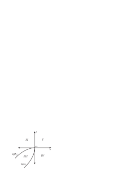
Figure 2.1. A partition of the $rs-$plane into four sections: $I$, $II$, $III$ and $IV$.

Consider $\mathcal{T}_{1}(\overline{U}_{L})$. For each $\overline{U}_{M}\in\mathcal{T}_{1}(\overline{U}_{L})$ the 3-wave rarefaction curves based at $\overline{U}_{M}$ extend vertically upwards, parallel to the $s-$axis. Therefore, for all states $\overline{U}_{R}$ in region $I$ or $II$, there is a unique state $\overline{U}_{M}\in\mathcal{T}_{1}(\overline{U}_{L})$ that connects $\overline{U}_{L}$ to $\overline{U}_{R}$ by a $1-$shock or a $1-$rarefaction wave followed by a $3-$rarefaction wave.

We now turn our attention to the portion below $\mathcal{T}_{1}(\overline{U}_{L})$ in the $rs-$plane. For region $IV$, we notice for any state $\overline{U}_{1}\in\mathcal{R}^{+}_{1}(\overline{U}_{L})$ the shock curve $\mathcal{S}^{-}_{3}(\overline{U}_{1})$ is a horizontal translation of $\mathcal{S}^{-}_{3}(\overline{U}_{L})$. Thus, all the $3-$shock curves extending from $\mathcal{R}^{+}_{1}(\overline{U}_{L})$ cover region $IV$. For region $III$ it is clear that the $3-$shock curves extending downward from $\mathcal{S}^{-}_{1}(\overline{U}_{L})$ must cover all states in the region. But, we must show that if we take two states $\overline{U}_{1}$ and $\overline{U}_{2}$ on the shock curve of $\overline{U}_{L}$ they will never intersect. Suppose two shock curves intersect at a third state $\overline{U}_{3}$. See Figure 2.2. We know by Lemma 2.7 that

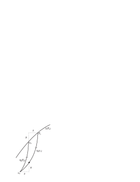
Figure 2.2. Possible Intersection of two $3-$Shock Curves.

$$\frac{z}{y}\leq\frac{\sqrt{2K}-1}{-\sqrt{2K}-1}<1.$$

However, if $\overline{U}_{1}$ and $\overline{U}_{2}$ are on the same shock curve,

$$\frac{y}{z}\leq\frac{\sqrt{2K}-1}{-\sqrt{2K}-1}<1.$$

It must be that the curves never intersect. Thus, we can solve the Riemann problem $<\overline{U}_{L},\overline{U}_{2}>$ in the $rs-$plane.

Now, we use this result to find a solution to the Riemann problem with $U_{L}=(\rho_{L},v_{L},S_{L})$ and $U_{R}=(\rho_{R},v_{R},S_{R})$. By the previous argument, find a middle state $(\rho_{M},v_{M})$ that solves the Riemann problem, $<(\rho_{L},v_{L}),(\rho_{L},v_{L})>$, in the $rs$-plane. We only need to find the two values of $S$ on either side of the contact discontinuity. This can be accomplished by determining the change in entropy, across the $1$ and $3-$waves then adapting these changes to the left and right values of S. For example, the left middle state $U_{M}$ would have entropy value $S_{L}$ if we had a $1-$rarefaction wave, and would have entropy value $S_{M}$, where $S_{M}-S_{L}$ equals the corresponding increase in $S$ across the shock wave. We can find the change in entropy by looking at the equation $\rho/n^{\gamma}=A(S)$ and solving for $S$. This is possible since $A$ is strictly monotone increasing away from zero. Similar methods determine the value of $S_{M}^{\prime}$ and the value of entropy in the right middle state. Since the entropy values of the middle states satisfy, $S_{L}\leq S_{M}$ and $S_{R}\leq S_{M}^{\prime}$, we have $S_{M},S_{M}^{\prime}>0$. The position of the entropy jump is determined by the particle path emanating from the initial discontinuity with speed $v_{M}$.

This construction determines the two unique states $U_{M}=(\rho_{M},v_{M},S_{M})$ and $U_{M}^{\prime}=(\rho_{M},v_{M},S_{M}^{\prime})$ that solves the Riemann problem in the region $\rho>0$, $-1<v<1$ and $S>0$. Figure 2.3. ∎

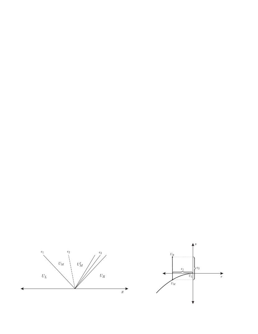
Figure 2.3. Solution to the Riemann Problem $<U_{L},U_{R}>$. The states $U_{M}$ and $U_{M}^{\prime}$ differ only in $S$.

We parameterize the $1-($resp. $3)$shock/rarefaction curve by the change in $r($resp. $s)$ and define the strength of a shock or rarefaction wave as the difference in the values of either $r$ for a $1-$shock-rarefaction wave, or $s$ for a $2-$shock-rarefaction wave. We choose the orientation on our parametrization so that we have a positive parameter along the rarefaction curve and negative parameter along the shock curve. Therefore, the solution of the Riemann problem can be given as a sequence of three coordinates, $(\epsilon_{1},\epsilon_{2},\epsilon_{3})$ where, $\epsilon_{1}$ denotes the change in the Riemann invariant $r$ from $U_{L}$ to $U_{M}$, $\epsilon_{2}$ the change in $S$ from $U_{M}$ to $U_{M}^{\prime}$ and $\epsilon_{3}$ the change in the Riemann invariant $s$ from $U_{M}^{\prime}$ to $U_{R}$. In summary, for $i=1,3$ we have a shock wave of strength $\epsilon_{i}$ when $\epsilon_{i}<0$ and a rarefaction wave of strength $\epsilon_{i}$ when $\epsilon_{i}>0$.

We adopt the following notation:

$$\alpha \textrm{Strength of }1-\textrm{Shock Wave}$$

$$\beta \textrm{Strength of }3-\textrm{Shock Wave}$$

$$\mu \textrm{Strength of }1-\textrm{Rarefaction Wave}$$

$$\eta \textrm{Strength of }3-\textrm{Rarefaction Wave}$$

$$\delta \textrm{Strength of Entropy}\phantom{3}\Sigma\textrm{-Wave}$$

If $(\epsilon_{1},\epsilon_{2},\epsilon_{3})$ is the solution to the Riemann problem with states $U_{L}$, $U_{R}$, we would have:

$$\alpha=\left\{\begin{array}[]{ll}-\epsilon_{1}\phantom{44444}&\epsilon_{1}\leq 0\\ 0&\textrm{Otherwise}\\ \end{array}\right.\phantom{44444}\beta=\left\{\begin{array}[]{ll}-\epsilon_{3}\phantom{44444}&\epsilon_{3}\leq 0\\ 0&\textrm{Otherwise}\\ \end{array}\right.$$

$$\mu=\left\{\begin{array}[]{ll}\epsilon_{1}\phantom{44444}&\epsilon_{1}\geq 0\\ 0&\textrm{Otherwise}\\ \end{array}\right.\phantom{44444}\eta=\left\{\begin{array}[]{ll}\epsilon_{3}\phantom{44444}&\epsilon_{3}\geq 0\\ 0&\textrm{Otherwise}\\ \end{array}\right.$$

We define $\delta=\Sigma_{R}-\Sigma_{L}$ where $\Sigma=\ln(A(S))$. The value of $S$ may be recovered by recalling this definition and since $\Sigma$ is a strictly increasing function of $S$ by (A3). Also, we will denote $\delta_{\omega}$ as the absolute change of $\Sigma$ across a shock wave of strength $\omega$. More specifically, if two states were separated by a shock of strength $\omega$ the absolute change in $\Sigma$ across the shock would be $\delta_{\omega}$ for either a $1$ or $3-$shock. Since we have shown that the change in $\Sigma$ is independent on the base state and dependent only on the strength of the wave, $\delta_{\omega}$ is well defined.

2.6. Interaction Estimates

In this section we prove estimates for elementary wave interactions with a method that follows the work by Nishida and Smoller, and Temple in [8] and [12]. This method is employed in order to simplify the estimates on the variation in the entropy. The alternative approach, useing the wave interaction potential $Var\left\{ln(\rho)\right\}$ introduced by Liu and used in [10], simplifies the estimates dealing with the first and third, nonlinear, characteristic classes, but complicates the estimates dealing with the entropy.

Consider the following three states, $U_{L}=(\rho_{L},v_{L},\Sigma_{L})$, $U_{M}=(\rho_{M},v_{M},\Sigma_{M})$, and $U_{R}=(\rho_{R},v_{R},\Sigma_{R})$. We wish to estimate the difference in the solutions of the three Riemann problems $<U_{L},U_{M}>$, $<U_{M},U_{R}>$, and $<U_{L},U_{R}>$ with solutions denoted by a $1$ subscript, $2$ subscript and ^′ respectively.

2.10 Proposition.

Let $\Omega$ be a simply connected compact set in $rs-$space. Then there exists a constant $C_{0}$, $1/2<C_{0}<1,$ such that for any interaction $<U_{L},U_{M}>+<U_{M},U_{R}>\rightarrow<U_{L},U_{R}>$ in $\Omega$ at any value of $\Sigma$, one of the following holds:

$$i.)\phantom{4} A=-\xi\leq 0,\phantom{333}0\leq B\leq C_{0}\xi,\phantom{33}$$

or

$$B=-\xi\leq 0,\phantom{333}0\leq A\leq C_{0}\xi,\phantom{33}$$

$$ii.)\phantom{4} A\leq 0,\textrm{ and }B\leq 0.\phantom{4444444444444}$$

Where $A=\alpha^{\prime}-\alpha_{1}-\alpha_{2}$ and $B=\beta^{\prime}-\beta_{1}-\beta_{2}$ are change in the strengths of the $1$ and $3$ shock waves in the solutions.

Here we note that after an interaction, the shock wave strength in one family may increase, but this increase is uniformly bounded by a corresponding decrease in shock strength for the opposite family.

Proof.

These estimates are proven in Chapter 5 by a systematic look at all possible wave interactions. Because the interactions are independent of entropy level, we only consider interactions within the first and third characteristic classes. There are sixteen unique incoming wave configurations and between one and four possible outgoing wave configurations. The main idea is that after an interaction, there cannot be an overall increase in the strengths of the shock waves. This fact follows since as the solution progresses forward in time, cancelations and merging of shock and rarefaction waves of the same class lead to a decrease in shock strength. For example, when a shock wave is weakened by a rarefaction wave, a reflected shock wave is created in the opposite family. This interaction may increase the total strength of the shock waves in the opposite family, but the total gain in shock strength is uniformly bounded by the loss in the weakened or annihilated shock.

We choose the constant $C_{0}$ to be the maximum slope of the largest shock wave curve that lies within the compact set $\Omega$ or $1/2$ in order to bound the constant below. More specifically, let $\overline{\omega}$ be the strongest largest shock wave possible in $\Omega$. Then we take $C_{0}$ to be

(2.27) $$C_{0}=\max\left\{\frac{1}{2},\left.\frac{dr}{ds}\right|_{\overline{\omega}},\left.\frac{ds}{dr}\right|_{\overline{\omega}}\right\}.$$

Finally, by Lemma 2.7, the slopes of the shock wave curves in a compact set in the $rs-$plane are strictly bounded away by $1$. Therefore, we conclude $C_{0}<1$. ∎

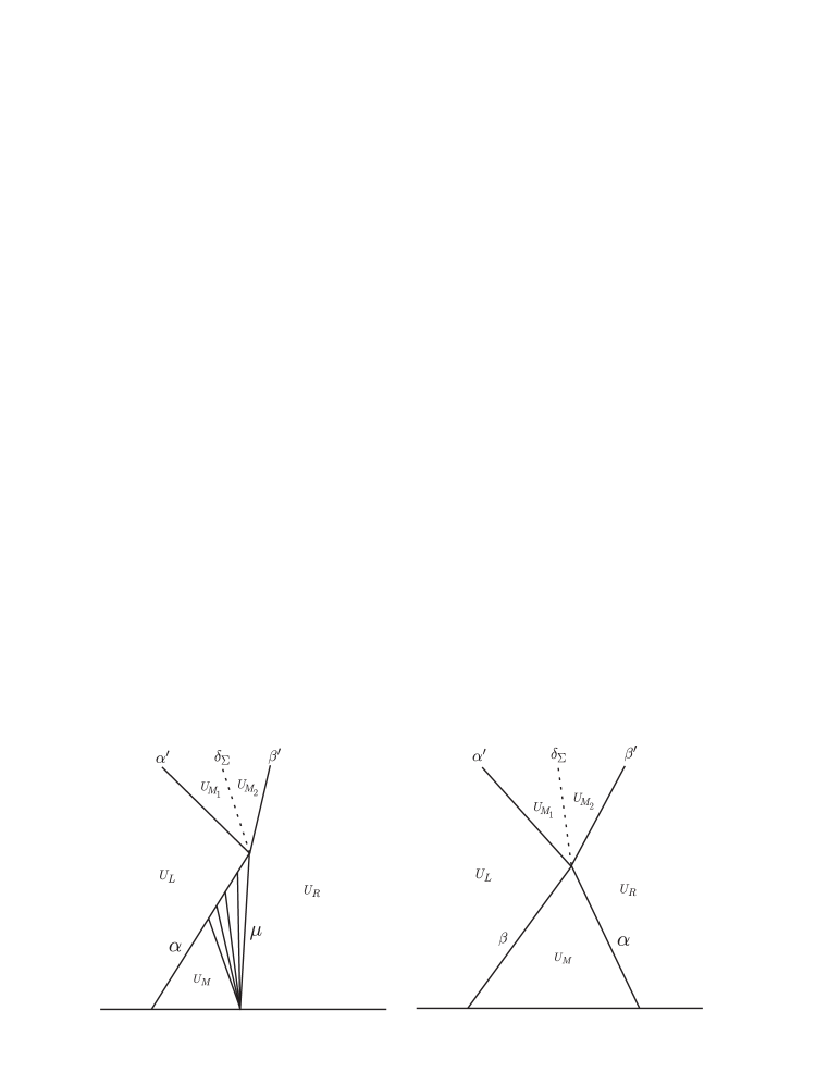
Figure 2.4. The creation of an entropy wave after elementary waves interact.

For interactions in a compact set, the variation in $\Sigma$ across a shock wave is uniformly bounded by a constant times the strength of the shock. But, the variation in $\Sigma$ may increase after an interaction because of the likely creation of an entropy wave. Typically, across these waves the pressure is invariant and there is a jump in density; however, under the assumption (1.10), there must be no jump in energy density. Thus, we cannot use $\ln\left(\rho/\rho_{L}\right)$ or the change in the Riemann invariants $r$ or $s$ as a measure of wave strength. It should be noted that under certain interactions, such as an $i-$shock being weakened by an incoming $i-$rarefaction wave, an entropy wave is created with strength such that $S_{M_{2}}-S_{M_{1}}$ is equal to the loss in entropy change across the shock, plus the change in the entropy across the new shock wave in the opposite family. We need a way to bound the variation in the entropy waves, and it turns out that this increase is bounded by a corresponding decrease in the shock strengths.

2.11 Proposition.

For every simply connected compact set $\Omega$ in $rs-$space, there exists a constant $M>0$ such that after every interaction in $\Omega$, at any value $\Sigma$ for the system (1.6) with (1.11) in the ultra-relativistic limit, the following holds:

$$|\delta^{\prime}|-|\delta_{1}|-|\delta_{2}|+(\delta_{\alpha_{1}}+\delta_{\alpha_{2}}-\delta_{\alpha^{\prime}})+(\delta_{\beta_{1}}+\delta_{\beta_{2}}-\delta_{\beta^{\prime}})\leq-M(A+B).$$

Proof.

Choose $C_{0}$ so that Proposition 2.10 holds. Since $\Omega$ is a compact set, let

$$\overline{\omega}=\sup\left\{\|(r_{1},s_{1})-(r_{2},s_{2})\|:(r_{1},s_{1}),(r_{2},s_{2})\in\Omega\right\}.$$

Then the strength of the largest shock wave in $\Omega$ is bounded by $\overline{\omega}$. Furthermore, let $M=\left(1-C_{0}\right)^{-1}\overline{M}$, where

(2.28) $$\overline{M}=2\frac{d[\Sigma-\Sigma_{L}]}{d\omega}(\overline{\omega}),$$

which is twice the largest rate of change of $\Sigma$ for all shocks contained in $\Omega$. Also, since $[\Sigma-\Sigma_{L}](\omega)$ is positive and convex up, we have for strengths, $\omega^{\prime}\geq\omega_{1}+\omega_{2}$, $\delta_{\omega^{\prime}}\geq\delta_{\omega_{1}}+\delta_{\omega_{2}}$.

The proof will be split into two cases, one for each of the two cases from Proposition 2.10. First let us assume that $A\leq 0$ and $B\leq 0$. i.e.

$$\alpha^{\prime}-\alpha_{1}-\alpha_{2}=-\xi_{\alpha}\leq 0\phantom{33}\textrm{and}\phantom{33}\beta^{\prime}-\beta_{1}-\beta_{2}=-\xi_{\beta}\leq 0.$$

We have, $\alpha_{1}+\alpha_{2}-\xi_{\alpha}=\alpha^{\prime}$ and hence, $\delta_{(\alpha_{1}+\alpha_{2}-\xi_{\alpha})}=\delta_{\alpha^{\prime}}$. It follows that

$$\delta_{\alpha_{1}}+\delta_{\alpha_{2}}-\frac{1}{2}\overline{M}\xi_{\alpha}\leq\delta_{\alpha_{1}+\alpha_{2}}-\frac{1}{2}\overline{M}\xi_{\alpha}\leq\delta_{\alpha^{\prime}}.$$

Rearranging,

(2.29) $$\delta_{\alpha_{1}}+\delta_{\alpha_{2}}-\delta_{\alpha^{\prime}}\leq\frac{1}{2}\overline{M}\xi_{\alpha}\leq-\frac{1}{2}MA,$$

and similarly,

(2.30) $$\delta_{\beta_{1}}+\delta_{\beta_{2}}-\delta_{\beta^{\prime}}\leq\frac{1}{2}\overline{M}\xi_{\beta}\leq-\frac{1}{2}MB.$$

The right hand inequalities follow from the fact that $\overline{M}<M$. Also, the change in entropy across the two Riemann problems before and the resulting one are equal:

(2.31) $$\delta_{\alpha^{\prime}}+\delta^{\prime}-\delta_{\beta^{\prime}}=\delta_{\alpha_{1}}+\delta_{1}-\delta_{\beta_{1}}+\delta_{\alpha_{2}}+\delta_{2}-\delta_{\beta_{2}}.$$

Rearranging (2.31) and using the previous estimates (2.29) and (2.30), we find

(2.32) $$\left(\delta^{\prime}-\delta_{1}-\delta_{2}\right)+\left(\delta_{\beta_{1}}+\delta_{\beta_{2}}-\delta_{\beta^{\prime}}\right)=\left(\delta_{\alpha_{1}}+\delta_{\alpha_{2}}-\delta_{\alpha^{\prime}}\right)\leq-\frac{1}{2}MA$$

and

(2.33) $$\left(\delta^{\prime}-\delta_{1}-\delta_{2}\right)+\left(\delta_{\alpha^{\prime}}-\delta_{\alpha_{1}}-\delta_{\alpha_{2}}\right)=\left(\delta_{\beta^{\prime}}-\delta_{\beta_{1}}-\delta_{\beta_{2}}\right)\geq\frac{1}{2}MB.$$

Adding the inequality (2.29) to (2.32),

$$\left(\delta^{\prime}-\delta_{1}-\delta_{2}\right)+\left(\delta_{\alpha_{1}}+\delta_{\alpha_{2}}-\delta_{\alpha^{\prime}}\right)+\left(\delta_{\beta_{1}}+\delta_{\beta_{2}}-\delta_{\beta^{\prime}}\right)\leq-\frac{1}{2}MA-\frac{1}{2}MA=-MA,$$

and adding $-1$ times the inequality (2.30) to (2.33),

$$\left(\delta^{\prime}-\delta_{1}-\delta_{2}\right)+\left(\delta_{\alpha^{\prime}}-\delta_{\alpha_{1}}+\delta_{\alpha_{2}}\right)+\left(\delta_{\beta^{\prime}}-\delta_{\beta_{1}}-\delta_{\beta_{2}}\right)\geq\frac{1}{2}MB+\frac{1}{2}MB=MB.$$

Therefore, after multiplying the entire inequality by $-1$ we have

$$-\left(\delta^{\prime}-\delta_{1}-\delta_{2}\right)+\left(\delta_{\alpha_{1}}+\delta_{\alpha_{2}}-\delta_{\alpha^{\prime}}\right)+\left(\delta_{\beta_{1}}+\delta_{\beta_{2}}-\delta_{\beta^{\prime}}\right)\leq-MB.$$

Since $0\leq-MA$ and $0\leq-MB$ by assumption, it follows that

$$|\delta^{\prime}-\delta_{1}-\delta_{2}|+\left(\delta_{\alpha_{1}}+\delta_{\alpha_{2}}-\delta_{\alpha^{\prime}}\right)+\left(\delta_{\beta_{1}}+\delta_{\beta_{2}}-\delta_{\beta^{\prime}}\right)\leq-M(A+B).$$

Furthermore, since $|\delta^{\prime}-\delta_{1}-\delta_{2}|\geq|\delta^{\prime}|-|\delta_{1}|-|\delta_{2}|$, we deduce,

$$|\delta^{\prime}|-|\delta_{1}|-|\delta_{2}|+\left(\delta_{\alpha_{1}}+\delta_{\alpha_{2}}-\delta_{\alpha^{\prime}}\right)+\left(\delta_{\beta_{1}}+\delta_{\beta_{2}}-\delta_{\beta^{\prime}}\right)\leq-M(A+B).$$

This concludes the proof of the first case.

Now, without loss of generality assume $A=-\xi\leq 0$ and $0\leq B\leq C_{0}\xi$. The mirror case when $0\leq A$ is similar. As before, we can obtain the estimates,

$$\delta_{\alpha_{1}}+\delta_{\alpha_{2}}-\delta_{\alpha^{\prime}}\leq\frac{1}{2}\overline{M}\xi$$

and

(2.34) $$\left(\delta^{\prime}-\delta_{1}-\delta_{2}\right)+\left(\delta_{\alpha_{1}}+\delta_{\alpha_{2}}-\delta_{\alpha^{\prime}}\right)+\left(\delta_{\beta_{1}}+\delta_{\beta_{2}}-\delta_{\beta^{\prime}}\right)\leq\overline{M}\xi.$$

From (2.31) we have,

$$-\left(\delta^{\prime}-\delta_{1}-\delta_{2}\right)+\left(\delta_{\alpha_{1}}+\delta_{\alpha_{2}}-\delta_{\alpha^{\prime}}\right)+\left(\delta_{\beta^{\prime}}-\delta_{\beta_{1}}+\delta_{\beta_{2}}\right)=0,$$

and since $\beta^{\prime}\geq\beta_{1}+\beta_{2}$, we have $\delta_{\beta_{1}}+\delta_{\beta_{2}}-\delta_{\beta^{\prime}}\leq 0$, and so by adding this inequality twice,

(2.35) $$-\left(\delta^{\prime}-\delta_{1}-\delta_{2}\right)+\left(\delta_{\alpha_{1}}+\delta_{\alpha_{2}}-\delta_{\alpha^{\prime}}\right)+\left(\delta_{\beta_{1}}+\delta_{\beta_{2}}-\delta_{\beta^{\prime}}\right)\leq 0.$$

Therefore, from (2.34) and (2.35),

$$|\delta^{\prime}-\delta_{1}-\delta_{2}|+\left(\delta_{\alpha_{1}}+\delta_{\alpha_{2}}-\delta_{\alpha^{\prime}}\right)+\left(\delta_{\beta_{1}}+\delta_{\beta_{2}}-\delta_{\beta^{\prime}}\right)\leq\overline{M}\xi,$$

which as before, reduces to,

$$|\delta^{\prime}|-|\delta_{1}|-|\delta_{2}|+\left(\delta_{\alpha_{1}}+\delta_{\alpha_{2}}-\delta_{\alpha^{\prime}}\right)+\left(\delta_{\beta_{1}}+\delta_{\beta_{2}}-\delta_{\beta^{\prime}}\right)\leq\overline{M}\xi.$$

But,

$$\overline{M}\xi=M(1-C_{0})\xi=M(\xi-C_{0}\xi)\leq M(-A-B)=-M(A+B),$$

where we used the fact $-C_{0}\xi\leq-B$ following from the assumption that $0\leq B\leq C_{0}\xi$ and $A=-\xi$. ∎

Chapter 3 The Glimm Difference Scheme

3.1. Introduction

In $1965$, Glimm proved existence of solutions to general systems of strictly hyperbolic conservation laws with genuinely non-linear or linearly degenerate characteristic fields, [4]. To obtain existence, Glimm needed to restrict to initial data with sufficiently small total variation to avoid having to rule out the possibility that the complicated, global nonlinear structure of the conservation law might create finite time blow up of the solution or approximation scheme. His method takes a piecewise constant approximate solution at one time step and uses numerous solutions to Riemann problems, defined at each point of discontinuity, to evolve the solution to a later time. After the approximate solution is brought forward in time, the solution is randomly sampled and a new piecewise constant approximate solution is obtained. A fascinating consequence is that one cannot choose any sequence of sample points to choose the states used for the new piecewise constant function at each time step, but rather must sample outside a set of measure zero in the space of all possible choices.

One way this scheme may break down for general systems of hyperbolic conservation laws is that Riemann problems may not have solutions if the initial left and right states are sufficiently far apart. A canonical example of this phenomenon occurs in the $p-$system which models a classical isentropic gas in Lagrangian coordinates. For this system, if the difference in velocity of the two initial states is sufficiently large, all the gas will be pulled from the region in between the two states forming a vacuum, [9]. This possible complication and issues with large scale non-linearities, led Glimm to prove existence for initial data with small variation. He showed that in this case, the total possible increase in variation in the approximate solution is bounded by a corresponding decrease in a quadratic functional. Thus, having a bound on the total variation in the solution showed that the Riemann problems used in evolving the approximate solution can be defined for all time.

In our case we prove a large data existence theorem; there is no restriction on the “smallness” of the initial conditions. In our existence proof, we will not need to use a quadratic functional to bound the total variation, because the geometric structure of the shock and rarefaction curves in $rs-$space do not allow the approximate solution to behave badly in the large. In this section, we will introduce the Glimm scheme and use it to construct solutions to (1.6).

3.2. Glimm Difference Scheme

We say $U(x,t)$ is a weak solution of (1.6) with initial data $U_{0}(x)$, if for all $\varphi\in\mathcal{C}_{0}^{1}\left[\mathbb{R}^{+},\mathbb{R}\right]$ the following holds:

$$\int_{0}^{\infty}\!\!\int_{-\infty}^{\infty}U\varphi_{t}+F(U)\varphi_{x}dxdt+\int_{-\infty}^{\infty}U(x,0)\varphi(x,0)dx=0.$$

We begin by partitioning space into intervals of length $\Delta x$ and time into intervals of length $\Delta t$. In order to keep neighboring Riemann problems from colliding, we impose the following CFL condition:

$$\frac{\Delta x}{\Delta t}>1>|\lambda_{i}|,\phantom{333}i=1,2,3.$$

Note for $1<\gamma<2$ this condition is satisfied since the characteristic speeds (2.5) are bounded above and below by $1$ and $-1$.

We inductively define our approximate solution. To begin suppose that we have an approximate solution at time $t=n\Delta t$, $U(x,n\Delta t)$, which is constant on the intervals, $\left(k\Delta x,(k+2)\Delta x\right)$, where $k+n$ is odd. At each point $x=k\Delta x$ a Riemann problem is defined. Solve each Riemann problem for time $t=\Delta t$. This evolves our approximate solution from $t=n\Delta t$ to $t=(n+1)\Delta t$. To finish, we must construct a new piecewise constant function at time $t=(n+1)\Delta t$. Choose $a\in\left[-1,1\right]$ and define, $U(x,(n+1)\Delta t)=U((k+1+a)\Delta x,(n+1)\Delta t-)$ for $x\in(k\Delta x,(k+2)\Delta x)$ and $k+n+1$ odd. The term $\Delta t-$ denotes the lower limit.

Figure 3.1. Construction of Piecewise Constant Function

To begin this process at $t=0$, obtain a piecewise constant function from the initial data $U_{0}(x)$ by again choosing $a\in\left[-1,1\right]$ and defining, $U(x,0)=U_{0}((k+a)\Delta x)$ for $k$ odd.

Consider, $\theta\in\prod_{i=0}^{\infty}\left[-1,1\right]$. In other words, $\theta=\left(\theta_{0},\theta_{1},\ldots,\theta_{n},\ldots\right)$ with $\theta_{i}\in\left[-1,1\right]$. Then, for initial data, we say $U_{\theta,\Delta x}(x,t)$ is the approximate solution given by a mesh size of $\Delta x$ with sampling points at the $n^{\textrm{th}}$ time step given by $\theta_{n}$.

Figure 3.2. I-Curve $J$.

In order to estimate the change in the variation of our approximate solutions, we will define piecewise linear, space-like curves, called I-curves, which connect sample points at different time levels. If an I-curve $J$ passes through the sampling point $((k+\theta_{n})\Delta x,n\Delta t)$, then on the right $J$ is only allowed to connect to $((k+1+\theta_{n\pm 1})\Delta x,(n\pm 1)\Delta t)$ and on the left to $((k-1+\theta_{n\pm 1})\Delta x,(n\pm 1)\Delta t)$.

We consider two functionals defined on $I-$curves and will analyze how the functionals change as we change from one $I-$curve to another. This will allow us to estimate the change in variation of the approximate solution as it is evolved using the Glimm scheme. We define for an $I-$curve $J$:

(3.1) $$F(J)=\sum_{J}\alpha_{i}+\sum_{J}\beta_{i}+V$$

and

(3.2) $$L(J)=\sum_{J}\left(\alpha_{i}-M_{0}\delta_{\alpha_{i}}\right)+\sum_{J}\left(\beta_{i}-M_{0}\delta_{\beta_{i}}\right)-M_{0}\sum_{j}|\delta|+V,$$

where the sums are taken over all waves, or fractions of them in the case of rarefaction waves, that cross $J$. The constant $M_{0}$ will be chosen later and $V=Var\left\{U_{0}(\cdot)\right\}$ is the variation of the initial data.

The main problem in our analysis is to show that the variation in the entropy waves stays bounded for all time. To do this we need to bound the possible change in $\Sigma$ across shock waves. This is accomplished by first showing that the variation in $r$ and $s$ stays finite for all time. This implies that all the interactions, as projected onto the $rs-$plane, occur in a compact set. Thus, there is a largest possible shock strength in this compact set, and using the fact that the derivative of the entropy change as a function of wave strength is monotone increasing, there is a constant such that the entropy change is bounded by a constant times the wave strength. Moreover, we can then use Proposition 2.11 to estimate the increase in the variation in entropy in our approximate solutions.

3.3. Estimates on Approximate Solutions

For initial data $U_{0}(x)$ and corresponding approximate solution $U_{\theta,\Delta x}(x,t)$, define $\overline{U}_{0}(x)$ and $\overline{U}_{\theta,\Delta x}(x,t)$ as the initial data and approximate solutions viewed as functions of $r$ and $s$ only. The first estimate will show that the variation in the Riemann invariants across an I-curve $J$ is bounded above by the functional $F(\cdot)$ on $J$.

3.1 Proposition.

Let $\overline{U}_{0}(\cdot)$ be of finite variation. If the approximate solution $\overline{U}_{\theta,\Delta x}(x,t)$ is defined on an I-curve $J$, then,

(3.3) $$Var_{rs}(J)\leq 4F(J).$$

Proof.

Let $Var^{-}_{r}(J)$ denote the variation across $J$ given by a decrease in $r$. The only waves that contribute to the decrease in $r$ are $1$ and $3-$shocks. Furthermore, we have

(3.4) $$Var_{r}^{-}(J)\leq\sum_{J}\alpha_{i}+\sum_{J}\beta_{i},$$

where the sum is over all waves of the particular type crossing $J$. We can similarly define $Var^{+}_{r}(J)$ as the variation given by increases of $r$ across elementary waves. The only increase is given by $1-$rarefaction waves,

(3.5) $$Var_{r}^{+}(J)=\sum_{J}\mu_{i}.$$

Following this line of reasoning for $s$, we also have

(3.6) $$Var_{s}^{-}(J)\leq\sum_{J}\alpha_{i}+\sum_{J}\beta_{i}$$

and

(3.7) $$Var_{s}^{+}(J)=\sum_{J}\eta_{i}.$$

The initial data $\overline{U}_{0}$ may be written as a function of the Riemann invariants $r$ and $s$, $\overline{U}_{0}(x)=(r_{0}(x),s_{0}(x))$. Since $\overline{U}_{0}(\cdot)$ is of finite variation, the following limits must exist:

$$\lim_{x\rightarrow\pm\infty}r_{0}(x)=r^{\pm},\phantom{444}\lim_{x\rightarrow\pm\infty}s_{0}(x)=s^{\pm}.$$

Indeed, let $\{x_{n}\}_{n=0}^{\infty}$ be an increasing sequence of real numbers such that $x_{n}\rightarrow\infty$ as $n\rightarrow\infty$. Then,

$$\sum_{n=1}^{\infty}|r_{0}(x_{n})-r_{0}(x_{n-1})|\leq Var\{\overline{U}_{0}(\cdot)\}<\infty.$$

Hence the sequence $r_{0}(x_{n})$ is Cauchy, which converges to a finite limit $r^{+}$. The other cases are entirely similar.

For any I-curve $J$, the end states at $\pm\infty$ are given by $(r^{\pm},s^{\pm})$. From this we obtain

$$|Var^{+}_{r}(J)-Var^{-}_{r}(J)|=|r^{+}-r^{-}|\leq V,$$

and hence,

$$Var^{+}_{r}(J)\leq Var^{-}_{r}(J)+V.$$

Using $(\ref{eqn-VarrMinus-al-be})$ and $(\ref{eqn-VarrPlus-mu})$,

$$\sum_{J}\mu_{i}\leq\sum_{J}\alpha_{i}+\sum_{J}\beta_{i}+V.$$

Similarly from $(\ref{eqn-VarsMinus-al-be})$ and $(\ref{eqn-VarsPlus-eta})$,

$$\sum_{J}\eta_{i}\leq\sum_{J}\alpha_{i}+\sum_{J}\beta_{i}+V.$$

Combining these together we have,

$$\sum_{J}\mu_{i}+\sum_{J}\eta_{i}\leq 2\left(\sum_{J}\alpha_{i}+\sum_{J}\beta_{i}+V\right).$$

Thus,

$$Var_{rs}(J) \leq 2\left(\sum_{J}\alpha_{i}+\sum_{J}\beta_{i}\right)+\sum_{J}\mu_{i}+\sum_{J}\eta_{i},$$

$$\leq 4\left(\sum_{J}\alpha_{i}+\sum_{J}\beta_{i}\right)+2V,$$

$$\leq 4\left(\sum_{J}\alpha_{i}+\sum_{J}\beta_{i}+V\right),$$

$$\leq 4F(J).\phantom{\left(\sum_{J}\alpha_{i}\right)}$$

∎

We will now show that the functional $F(\cdot)$ on the I-curves is non-increasing. We define a partial ordering on the I-curves by saying that $J\prec J^{\prime}$ if the curve $J^{\prime}$ never lies below the curve $J$. Furthermore, we say that $J^{\prime}$ is an immediate successor to $J$ if $J\prec J^{\prime}$ and $J$ and $J^{\prime}$ share all the same sample points except for one. It is clear that for any pair of I-curves such that $J\prec J^{\prime}$, there is a sequence of immediate successors that begins at $J$ and ends at $J^{\prime}$. The next proposition shows that if our approximate solution is defined on an I-curve, it can be defined for all following I-curves.

3.2 Proposition.

Let $J$ and $J^{\prime}$ be $I-$curves, $J\prec J^{\prime}$, and suppose that $J$ is in the domain of definition of $\overline{U}_{\theta,\Delta x}$. If $F(J)<\infty$, then $J^{\prime}$ is in the domain of definition of $\overline{U}_{\Delta x,\theta}$, and $F(J^{\prime})\leq F(J)$. Moreover, if $Var_{rs}\left\{U_{0}(\cdot)\right\}<\infty$ then $\overline{U}_{\theta,\Delta x}$ can be defined for $t\geq 0$.

Figure 3.3. Immediate Successor I-Curves $J^{\prime}$ and $J$.

Proof.

We proceed by induction. Suppose first that $J^{\prime}$ is an immediate successor to $J$. Then the difference $F(J^{\prime})-F(J)$, is given by the change in shock wave strengths across the diamond enclosed by $J^{\prime}$ and $J$. See Figure 3.3. This is a consequence of the fact that the waves the head into the diamond from the left and right solve the same Riemann problem as the outgoing waves in the new single Riemann problem. If we denote $J^{\prime}_{0}$ and $J_{0}$ as the diamond portion of $J^{\prime}$ and $J$, we have,

$$F(J^{\prime})-F(J) = \sum_{J^{\prime}}\alpha_{i}+\sum_{J^{\prime}}\beta_{i}+V-\left(\sum_{J}\alpha_{i}+\sum_{J}\beta_{i}+V\right),$$

$$= \sum_{J_{0}^{\prime}}\alpha_{i}+\sum_{J_{0}^{\prime}}\beta_{i}-\sum_{J_{0}}\alpha_{i}-\sum_{J_{0}}\beta_{i},$$

$$= \left(\alpha^{\prime}-\alpha_{1}-\alpha_{2}\right)+\left(\beta^{\prime}-\beta_{1}-\beta_{2}\right),$$

$$= A+B\leq 0.$$

The last line follows from Proposition 2.10. Thus, $F(J^{\prime})\leq F(J)$ for immediate successors. For any a general $J$ and $J^{\prime}$ such that $J\prec J^{\prime}$, we produce a sequence of immediate successors that take $J$ to $J^{\prime}$. At each step the functional $F$ is non-increasing, thus $F(J^{\prime})\leq F(J)$ continues to hold.

By Proposition 3.1, $Var_{rs}(J^{\prime})\leq 4F(J^{\prime})\leq 4F(J)$, so, $J^{\prime}$ is in the domain of definition of $\overline{U}_{\theta,\Delta x}$. Moreover, if $Var_{rs}\left\{\overline{U}_{0}(\cdot)\right\}<\infty$, then $Var_{rs}(\mathbf{0})<\infty$ for the unique $I-$curve $\mathbf{0}$ that lies along the line $t=0$. In order to show that $\overline{U}_{\Delta x,\theta}$ can be defined for $t\geq 0$, we must show that $Var_{rs}\left\{\overline{U}_{\theta,\Delta x}(\cdot,t)\right\}<\infty$ for all time. But, this condition is equivalent to showing the variation across any $I-$curve $J$ is always finite. Since for any $I-$curve $J$,

$$Var_{rs}(J)\leq 4F(J)\leq 4F(\mathbf{0})\leq 8Var_{rs}\left\{U_{0}(\cdot)\right\},$$

the result follows. ∎

Again, Proposition 3.2 shows that the variation of our approximate solution in the variables $r$ and $s$ is finite. Thus, there exists a compact set in the $rs-$plane that contains all the interactions in our approximate solution.

3.3 Corollary.

Suppose that $Var_{rs}\left\{U_{0}(\cdot)\right\}<\infty$. Then there exists a simply connected compact set $\Omega$ in the $rs-$plane such that all possible interactions are contained in $\Omega$.

Proof.

From Proposition 3.1 and Proposition 3.2 we know that for any I-curve $J$,

$$Var_{rs}(J)<4F(J)<4F(\mathbf{0})<8Var_{rs}\left\{U_{0}(\cdot)\right\}=N<\infty.$$

Thus, the distance between any to states occurring anywhere in our approximate solution is bounded by $N$. Consider the left limit state of $\overline{U}_{0}(\cdot)$, $(r^{-},s^{-})$. Therefore, all states must be contained within, $B_{2N}(r^{-},s^{-})$, the ball of radius $2N$ centered around $(r^{-},s^{-})$. ∎

Now, we show that the variation of our approximate solution, including the variation in $\Sigma$, is bounded above by the functional $L(\cdot)$.

3.4 Proposition.

Suppose $Var\left\{U_{0}(\cdot)\right\}<\infty$ and $J$ is an $I-$curve that is in the domain of definition of $U_{\theta,\Delta x}$. Then there exists constants $M_{0}>0$ and $K>0$, independent of $\Delta x$ and $\theta$, such that,

(3.8) $$Var(J)\leq K\cdot L(J).$$

Proof.

The variation across the $I-$curve $J$ is bounded by

$$Var(J) \leq Var(\textrm{Shock Waves})+Var(\textrm{Rarefaction Waves})$$

$$+Var(\Sigma\textrm{-Waves})+Var(\Sigma\textrm{ across Shocks}).$$

Since $Var_{rs}\left\{\overline{U}_{0}(\cdot)\right\}\leq Var\left\{U_{0}(\cdot)\right\}<\infty$, we have from Corollary 3.3 that all the interactions projected into the $rs-$plane occur in a compact set $\Omega$. Therefore there exists a constant $\overline{M}>0$ such that for a shock wave of strength $\omega$, $\delta_{\omega}\leq\overline{M}\omega$. Let $M=(1-C_{0})^{-1}\overline{M}$ as in Proposition 2.11. Since, $\overline{M}<M$ we have for a shock wave of strength $\omega$, $\delta_{\omega}<M\omega$.

From the proof of Proposition 3.1, we can bound the variation from the shock waves and rarefaction waves by the shock waves crossing $J$ and the initial variation $V$. Thus,

$$Var(J) \leq 2\left(\sum_{J}\alpha_{i}+\sum_{J}\beta_{i}\right)+\sum_{J}\mu_{i}+\sum_{J}\eta_{i}\phantom{\left(\sum\right)}$$

$$\phantom{44444444}+\sum_{J}|\delta|+\sum_{J}\delta_{\alpha_{i}}+\sum_{J}\delta_{\beta_{i}},\phantom{\sum_{J}|\delta|}$$

$$\leq 4\left(\sum_{J}\alpha_{i}+\sum_{J}\beta_{i}+V\right)+\sum_{J}|\delta|+M\left(\sum_{J}\alpha_{i}+\sum_{J}\beta_{i}\right),$$

$$\leq (4+M)\left(\sum_{J}\alpha_{i}+\sum_{J}\beta_{i}+V\right)+\sum_{J}|\delta|.$$

Let $M_{0}\leq 1/2M$. Then,

$$M_{0}\delta_{\omega}\leq\frac{1}{2M}\delta_{\omega}\leq\frac{1}{2M}\left(M\omega\right)\leq\frac{1}{2}\omega.$$

Thus, for a shock wave of strength $\omega$,

$$\omega\leq 2(\omega-M_{0}\delta_{\omega}).$$

Using this, we find,

$$Var(J)\leq 2(4+M)\left(\sum_{J}\left(\alpha_{i}-M_{0}\delta_{\beta_{i}}\right)+\sum_{J}\left(\beta_{i}-M_{0}\delta_{\beta_{i}}\right)+V\right)+\sum_{J}|\delta|.$$

Finally, we put the sum of the strengths of the entropy waves inside,

$$Var(J)\leq 2(4+M)\left(\sum_{J}\left(\alpha_{i}-M_{0}\delta_{\beta_{i}}\right)+\sum_{J}\left(\beta_{i}-M_{0}\delta_{\beta_{i}}\right)+M_{0}\sum_{J}|\delta|+V\right).$$

We can do this because,

$$M_{0}\cdot 2(4+M)\geq 2MM_{0}\geq 1.$$

Therefore,

$$Var(J)\leq K\cdot L(J),$$

with $K=2(4+M)$. ∎

3.5 Proposition.

Suppose that $Var\left\{U_{0}(\cdot)\right\}<\infty$ and $J$, $J^{\prime}$ are I-curves such that $J\prec J^{\prime}$ and $L(J)<\infty$. Then $J^{\prime}$ is in the domain of definition of $U_{\theta,\Delta x}(x,t)$, $L(J^{\prime})\leq L(J)$ and $U_{\Delta x,\theta}(x,t)$ is defined for $t\geq 0$.

Proof.

Since $Var_{rs}\left\{\overline{U}_{0}(\cdot)\right\}<Var\left\{U_{0}(\cdot)\right\}<\infty$ there exists a compact set $\Omega$ that contains all possible interactions. Define $M$ as in Proposition 2.11 and take $M_{0}\leq 1/2M$. As with Proposition 3.2, we prove the result by induction on the $I$ curves. First let $J^{\prime}$ be an immediate successor to $J$. Let $J^{\prime}_{0}$ and $J_{0}$ be the parts of $J^{\prime}$ and $J$ that bound the diamond formed by $J$ and $J^{\prime}$. Using this and the definition of $L(J)$,

$$L(J^{\prime})-L(J) \leq \left[\sum_{J^{\prime}_{0}}\left(\alpha_{i}-M_{0}\delta_{\alpha_{i}}\right)+\sum_{J^{\prime}_{0}}\left(\beta_{i}-M_{0}\delta_{\beta_{i}}\right)+M_{0}\sum_{J^{\prime}_{0}}|\delta|\right]$$

$$\phantom{44}-\left[\sum_{J_{0}}\left(\alpha_{i}-M_{0}\delta_{\alpha_{i}}\right)+\sum_{J_{0}}\left(\beta_{i}-M_{0}\delta_{\beta_{i}}\right)+M_{0}\sum_{J_{0}}|\delta|\right],$$

$$= \left(\alpha^{\prime}-\alpha_{1}-\alpha_{2}\right)+\left(\beta^{\prime}-\beta_{1}-\beta_{2}\right)+M_{0}\left(\delta_{\alpha_{1}}+\delta_{\alpha_{2}}-\delta_{\alpha^{\prime}}\right)$$

$$+M_{0}\left(\delta_{\beta_{1}}+\delta_{\beta_{2}}-\delta_{\beta^{\prime}}\right)+M_{0}\left(|\delta^{\prime}|-|\delta_{1}|-|\delta_{2}|\right).$$

Now we refer to Proposition 2.10 and 2.11. We see that the first two terms are equal to $(A+B)$ and the others are bounded above by $-M(A+B)$. Putting this together,

$$L(J^{\prime})-L(J)\leq(A+B)-MM_{0}(A+B)\leq\frac{1}{2}(A+B)\leq 0.$$

For immediate successors, we have $L(J^{\prime})\leq L(J)$. Moreover, by Proposition 3.4 we have that the variation along $J^{\prime}$ is bounded by $L(J^{\prime})$ and hence $L(J)$. Thus, $J^{\prime}$ is in the domain of definition of $U_{\Delta x,\theta}$.

For general $J$ and $J^{\prime}$ such that $J\prec J^{\prime}$, the same conclusion holds by constructing a sequence of immediate successors to move from $J$ to $J^{\prime}$. Along each step, the results above continue to hold.

Finally, if $Var\left\{U_{0}(\cdot)\right\}<\infty$, we have $L(0)<\infty$ and for any $I-$curve $J$, $L(J)\leq L(0)$. Which we can conclude that

$$Var(J)\leq 2(4+M)L(J)\leq 2(4+M)L(0)<\infty,$$

so our approximate solution can be defined for $t\geq 0$. ∎

Chapter 4 Existence Theorem for Two Gasses

In this chapter, we use Glimm’s Theorem [4] to prove existence of solutions to (1.6) in the ultra-relativistic limit with an equation of state of the form (1.11). It should be noted that for $\theta$ fixed and $x_{n}=1/2^{n}$, the set of approximate solutions $\left\{U_{\theta,\Delta x_{n}}(x,t)\right\}^{\infty}_{n=1}$ has uniformly bounded variation by Proposition 3.4. Furthermore, since the variation is bounded and each approximate solution has the same limits at infinity, the sup norm is also uniformly bounded. The approximate solutions are $\mathbf{L}^{1}$ Lipschitz in time too since

$$\|U_{\theta,\Delta x}(\cdot,t)-U_{\theta,\Delta x}(\cdot,s)\|_{\mathbf{L}^{1}} \leq C\left\{\textrm{Sum of all wave strengths}\right\}\cdot$$

$$\phantom{4444}\left\{\textrm{Maximum Speed of Wavefronts}\right\}<C^{\prime}|t-s|.$$

At this point Helly’s Theorem [2] provides a convergent subsequence, $U_{\theta,\Delta x_{n_{i}}}(x,t)$, that converges to a function $U(x,t)$ with finite variation for each fixed time. However at this time, there is no justification that this limit function is actually a weak solution. Glimm’s Theorem guarantees that there exists a subsequence that converges to a weak solution.

4.1. Existence of Weak Solutions

3 Theorem (Glimm, $1965$).

Assume that the approximate solution $U_{\theta,\Delta x_{i}}$ satisfies,

(4.1) $$Var\left\{U_{\theta,\Delta x_{i}}(\cdot,t)\right\}<N<\infty$$

for $x_{i}=1/2^{i}$, $\theta\in A=\prod_{i=0}^{\infty}$, and all $t\geq 0$. Then there exits a subsequence of mesh lengths $\Delta x_{i_{k}}$ such that $U_{\theta,\Delta x_{i_{k}}}\rightarrow U$ in $\mathbf{L}^{1}_{Loc}$ where $U(x,t)$ satisfies,

$$Var\left\{U(\cdot,t)\right\}<N.$$

Furthermore, there exits a set of measure zero $\overline{A}\subset A$ such that if $\theta\in A-\overline{A}$ then $U(x,t)$ is a weak solution to (1.6).

We now prove Theorem 1 by showing that our approximate solutions meet the assumptions of Glimm’s Theorem.

Proof.

Assume the initial data satisfies, (1.14), (1.15), and (1.16) We will show that for all $\Delta x_{i}$ and sample points $\theta$,

(4.2) $$Var\left\{U_{\Delta x,\theta}(\cdot,t)\right\}<N<\infty,$$

where $U_{\theta,\Delta x}(\rho(x,t),v(x,t),S(x,t))=(U_{1},U_{2},U_{3})_{\theta,\Delta x}$. First we show that the variation in $\rho$, $v$, and $S$ is bounded for all time in the approximate solutions.

From Proposition 3.1 and Proposition 3.2 we have that the variation of our approximate solution in $r$ and $s$ is uniformly bounded for all time. More specifically,

$$Var_{rs}\left(\overline{U}_{\theta,\Delta x}(\cdot,t)\right) < 4F(\mathbf{0}),$$

$$< 4\left[\sum_{\mathbf{0}}\alpha_{i}+\sum_{\mathbf{0}}\beta_{i}+Var_{rs}(U_{0})\right],$$

$$< 8\cdot Var_{rs}(U_{0}(\cdot)).$$

From this estimate, we show that the variation of

$$\ln\left(\rho\right)\phantom{4444}\textrm{and}\phantom{4444}\ln\left(\frac{1+v}{1-v}\right)$$

are also bounded for all time. Indeed by the definition of $r$ and $s$,

$$\ln\left(\frac{1+v}{1-v}\right)=\frac{1}{2}(r+s),$$

we have

$$Var\left\{\ln\left(\frac{1+v(\cdot,t)}{1-v(\cdot,t)}\right)\right\} = \frac{1}{2}\sup_{N}\sum_{i=1}^{N}|(r(x_{i+1},t)+s(x_{i+1},t))-(r(x_{i},t)+s(x_{i},t))|,$$

$$\leq \frac{1}{2}\sup_{N}\sum_{i=1}^{N}|r(x_{i+1},t)-r(x_{i},t)|$$

$$\phantom{4444444}+\frac{1}{2}\sup_{N}\sum_{i=1}^{N}|s(x_{i+1},t)-s(x_{i},t)|,$$

$$\leq \frac{1}{2}Var_{rs}\left\{\overline{U}_{\Delta x,\theta}(\cdot,t)\right\}+\frac{1}{2}Var_{rs}\left\{\overline{U}_{\Delta x,\theta}(\cdot,t)\right\},$$

$$\leq 8\cdot Var\left\{U_{0}(\cdot)\right\}.$$

Similarly, using

$$\ln(\rho)=\frac{1+a^{2}}{a}(s-r),$$

we find,

$$Var\left\{\ln(\rho(\cdot,t))\right\}\leq 16\left(\frac{1+a^{2}}{a}\right)Var\left\{U_{0}(\cdot)\right\}.$$

Now, we show the variation in $\Sigma$ is bounded for all time in approximate solutions. This is clear from Proposition 3.4 and Proposition 3.5 because there exists a constant $M$ so that

$$Var\left\{\Sigma_{\theta,\Delta x}(\cdot,t)\right\}\leq 2(4+M)L(\mathbf{0}).$$

We can now show that the variation in $\rho$, $v$ and $S$ is bounded for all time. Since $Var\left\{\ln(\rho(\cdot,t))\right\}<\infty$ for all $t>0$ there exists a constant $b>0$ such that $\rho(x,t)<b$. Let $c=max\left\{1,b\right\}$, then

$$Var\left\{\rho(\cdot,t)\right\} = \sup_{N}\sum_{i=1}^{N}|\rho(x_{i+1},t)-\rho(x_{i},t)|,$$

$$\leq c\cdot\sup_{N}\sum_{i=1}^{N}|\ln(\rho(x_{i+1},t))-\ln(\rho(x_{i},t))|,$$

$$\leq c\cdot Var\left\{\ln(\rho(\cdot,t))\right\}.$$

For $v$ we have,

$$Var\left\{v(\cdot,t)\right\} = \sup_{N}\sum_{i=1}^{N}\left|v(x_{i+1},t)-v(x_{i},t)\right|,$$

$$\leq \frac{1}{2}\sup_{N}\sum_{i=1}^{N}\left|\ln\left(\frac{1+v(x_{i+1},t)}{1-v(x_{i+1},t)}\right)-\ln\left(\frac{1+v(x_{i},t)}{1-v(x_{i},t)}\right)\right|,$$

$$\leq \frac{1}{2}Var\left\{\ln\left(\frac{1+v(\cdot,t)}{1-v(\cdot,t)}\right)\right\}.$$

The factor $1/2$ comes from the fact that the slope of the chord connecting the points,

$$\left(v(x_{i+1},t),\ln\left(\frac{1+v(x_{i+1},t)}{1-v(x_{i+1},t)}\right)\right)\phantom{333}\textrm{and}\phantom{333}\left(v(x_{i},t),\ln\left(\frac{1+v(x_{i},t)}{1-v(x_{i},t)}\right)\right)$$

is bounded below by $2$.

For $S$ we need to find a constant $C$ such that

$$\left|S(x,t)-S(y,t)\right|\leq C\left|\Sigma(x,t)-\Sigma(y,t)\right|.$$

Since $\Sigma$ is of finite variation for all time, there exists a largest and smallest value of $S$, say $S_{max}$ and $S_{min}$ with $0<S_{min}\leq S_{max}$. Define $C$ by

$$C=max_{S\in\left[S_{min},S_{max}\right]}\left(\frac{d\Sigma}{dS}\right)^{-1}=max_{S\in\left[S_{min},S_{max}\right]}\frac{A(S)}{A^{\prime}(S)}.$$

It follows that,

$$Var\left\{S(\cdot,t)\right\}\leq C\cdot Var\left\{\Sigma(\cdot,t)\right\}.$$

Finally, from Proposition 2.5 the determinant of the Jacobian is bounded away from zero for all approximate solutions. Therefore, the variation in conserved variables, $(U_{1},U_{2},U_{3})$, are bounded for all $t\geq 0$, $\theta$ and $\Delta x_{i}$.

Therefore, Theorem 3 provides existence of a set measure zero $\overline{A}\subset A$ such that if we choose $\theta\in A-\overline{A}$ there exists a subsequence of mesh refinements, $\Delta x_{i_{k}}\to 0$ such that $U_{\theta,\Delta_{x_{i_{k}}}}$ converges pointwise almost everywhere in $L^{1}_{loc}$ to a weak solution, $U(x,t)$ of (1.6). Moreover, this solution satisfies

$$Var\left\{\ln(\rho(\cdot,t))\right\}<N,$$

$$Var\left\{\ln\left(\frac{1+v(\cdot,t)}{1-v(\cdot,t)}\right)\right\}<N,$$

and

$$Var\left\{S(\cdot,t)\right\}<N,$$

for some $N>0$, all $t>0$ and is $L^{1}$ Lipschitz in time.

∎

Chapter 5 Interaction Estimates

We give a systematic approach to the wave interaction estimates needed to prove Proposition 2.10. From the special geometry of the shock-rarefaction curves in the space of Riemann invariants we can analyze the interactions as done for the classical Euler equations in [8] and [12]. There are sixteen possible incoming wave profiles, and among these one to four different outgoing wave profiles, each of which will be covered on a case by case basis. We assume that all the interactions occur in a simply connected compact set $\Omega\subset\mathbb{R}^{2}$. Recall that for a compact set $\Omega$ we have defined the constant $C_{0}$, (2.27), as the max of $1/2$ or the largest slope possible of a shock curve contained in $\Omega$. Since the shock wave slopes are strictly bounded above by $1$, we have, $0<1/2\leq C_{0}<1$.

During these estimates we repeatedly use the fact that the shock curves in the space of Riemann invariants are translationally invariant, convex and whose derivatives are bounded above by a constant. We reference Lemma 2.7 for these results. Since our definition of wave strength is determined by the change in $r$ for $1-$waves and $s$ for $3-$waves, we use the following two facts:

1. The change in $s$ along a $1-$shock is uniformly bounded by the change in $r$ and vice versa for $3-$shocks. Indeed, since we have

   $$\frac{ds}{dr}\leq\frac{\sqrt{2K}-1}{-\sqrt{2K}-1}$$

   for $1-$shocks and

   $$\frac{dr}{ds}\leq\frac{\sqrt{2K}-1}{-\sqrt{2K}-1}$$

   for $3-$shocks, we have for our constant $C_{0}$,

   $$\frac{y_{1}}{z_{1}}<C_{0}\phantom{333}\textrm{and}\phantom{333}\frac{y_{3}}{z_{3}}<C_{0}.$$

   See Figure 5.1.

   

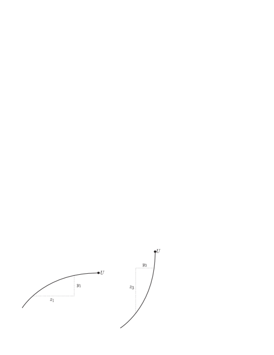
   Figure 5.1. Shock Curve Slopes are bounded by $C_{0}$.

2. Suppose two shock curves of the same family that begin at two distinct states $U_{1}$ and $U_{2}$ and meet at a common third state $U_{3}$. Then the ratio of the distances along the $r$ and $s$ axes from $U_{1}$ and $U_{2}$ are bounded by $C_{0}$. Again, we have,

   $$\frac{y_{1}}{z_{1}}<C_{0}\phantom{333}\textrm{and}\phantom{333}\frac{y_{3}}{z_{3}}<C_{0}.$$

   See Figure 5.2.

   

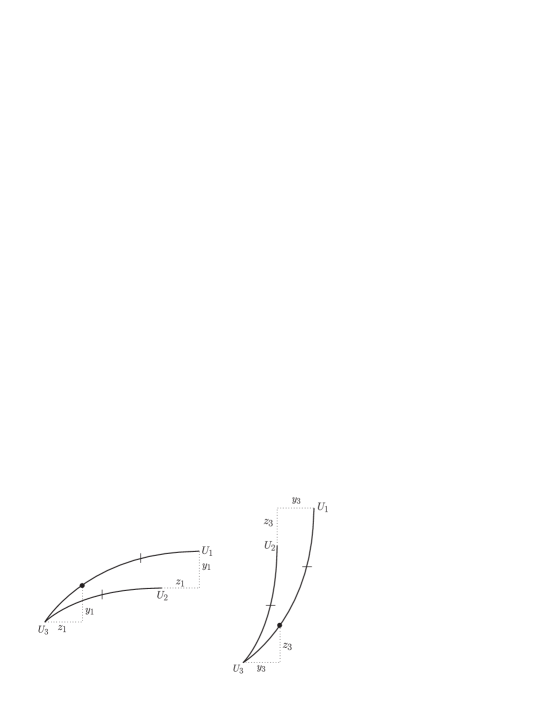
   Figure 5.2. Shock curves intersecting at $U_{3}$ satisfy, $y/z<C_{0}$.

We now begin our interaction analysis.

1. $(\alpha_{1},\beta_{1})+(\alpha_{2},\beta_{2})$

   • If $A\leq 0$ and $B\leq 0$ we are done.

     

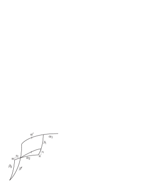
     Figure 5.3. $(\alpha_{1},\beta_{1})+(\alpha_{2},\beta_{2})\rightarrow(\alpha^{\prime},\beta^{\prime})$, $A\leq 0$, $B\geq 0$

   • $(\alpha_{1},\beta_{1})+(\alpha_{2},\beta_{2})\rightarrow(\alpha^{\prime},\beta^{\prime})$: Figure 5.3
              Suppose that $A=-\xi\leq 0$ and $B\geq 0$. We have $A=y_{1}-z_{2}$ and $B=y_{2}-z_{1}$. From $A\leq 0$, $y_{2}>z_{1}$, and hence,

     $$y_{1}<z_{1}<y_{2}<z_{2}.$$

     Therefore,

     $$A+B = (y_{1}-z_{2})+(y_{2}-z_{1}),$$

     $$= (y_{1}+y_{2})-(z_{1}+z_{2}),$$

     $$\leq (C_{0}-1)(z_{1}+z_{2}),$$

     $$\leq (C_{0}-1)(z_{2}-y_{1}),$$

     $$\leq C_{0}\xi+A.$$

     Hence, $B\leq C_{0}\xi$. Note, the inequalities hold since $(C_{0}-1)<0$.

     

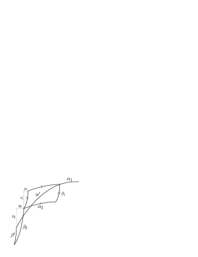
     Figure 5.4. $(\alpha_{1},\beta_{1})+(\alpha_{2},\beta_{2})\rightarrow(\alpha^{\prime},\beta^{\prime})$, $A\geq 0$, $B\leq 0$

   • $(\alpha_{1},\beta_{1})+(\alpha_{2},\beta_{2})\rightarrow(\alpha^{\prime},\beta^{\prime})$: Figure 5.4
              Suppose that $A\geq 0$ and $B=-\xi\leq 0$. We have $\alpha^{\prime}=\alpha_{1}+y_{1}+\alpha_{2}+y_{2}$ and hence, $A=\alpha^{\prime}-\alpha_{1}-\alpha_{2}=y_{1}+y_{2}$. Furthermore, $\beta^{\prime}+z_{2}+z_{1}=\beta_{1}+\beta_{2}$, which gives, $B=\beta^{\prime}-\beta_{1}-\beta_{2}=-z_{1}-z_{2}=-\xi$. Thus, $A\leq C_{0}\xi$.

     

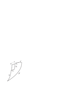
     Figure 5.5. $(\alpha_{1},\beta_{1})+(\alpha_{2},\beta_{2})\rightarrow(\mu^{\prime},\beta^{\prime})$

   • $(\alpha_{1},\beta_{1})+(\alpha_{2},\beta_{2})\rightarrow(\mu^{\prime},\beta^{\prime})$: Figure 5.5
     $A=-z$, $B=y\leq C_{0}z$.

     

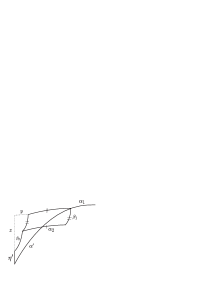
     Figure 5.6. $(\alpha_{1},\beta_{1})+(\alpha_{2},\beta_{2})\rightarrow(\alpha^{\prime},\eta^{\prime})$

   • $(\alpha_{1},\beta_{1})+(\alpha_{2},\beta_{2})\rightarrow(\alpha^{\prime},\eta^{\prime})$: Figure 5.6
     $B=-\beta_{1}-\beta_{2})=-z$, and $A=\alpha^{\prime}-\alpha_{1}-\alpha_{2}=y\leq C_{0}z$.

2. $(\alpha_{1},\beta_{1})+(\alpha_{2},\eta_{2})$

   

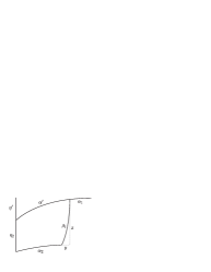
   Figure 5.7. $(\alpha_{1},\beta_{1})+(\alpha_{2},\eta_{2})\rightarrow(\alpha^{\prime},\eta^{\prime})$

   • $(\alpha_{1},\beta_{1})+(\alpha_{2},\eta_{2})\rightarrow(\alpha^{\prime},\eta^{\prime})$: Figure 5.7
               $B=-z$, $A=\alpha^{\prime}-\alpha_{1}-\alpha_{2}=y\leq C_{0}z$.

     

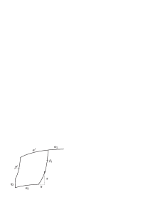
     Figure 5.8. $(\alpha_{1},\beta_{1})+(\alpha_{2},\eta_{2})\rightarrow(\alpha^{\prime},\beta^{\prime})$

   • $(\alpha_{1},\beta_{1})+(\alpha_{2},\eta_{2})\rightarrow(\alpha^{\prime},\beta^{\prime})$: Figure 5.8
               $B=\beta^{\prime}-\beta_{1}-\beta_{2}=-z$. Since, $\alpha_{1}+\alpha^{\prime}=\alpha_{2}+y+\alpha_{1}\Rightarrow\alpha^{\prime}-\alpha_{2}=y$ then, $A=\alpha^{\prime}-\alpha_{1}-\alpha_{2}\leq y\leq C_{0}z$.

   

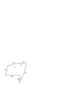
   Figure 5.9. $(\alpha_{1},\beta_{1})+(\mu_{2},\beta_{2})\rightarrow(\mu^{\prime},\beta^{\prime})$

3. $(\alpha_{1},\beta_{1})+(\mu_{2},\beta_{2})$

   • $(\alpha_{1},\beta_{1})+(\mu_{2},\beta_{2})\rightarrow(\mu^{\prime},\beta^{\prime})$: Figure 5.9
               $A=-\alpha_{1}=-z$, $B=\beta^{\prime}-\beta_{1}-\beta_{2}=y\leq C_{0}z$.

     

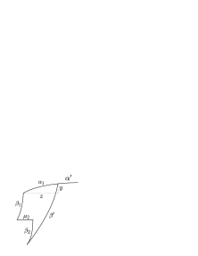
     Figure 5.10. $(\alpha_{1},\beta_{1})+(\mu_{2},\beta_{2})\rightarrow(\alpha^{\prime},\beta^{\prime})$

   • $(\alpha_{1},\beta_{1})+(\mu_{2},\beta_{2})\rightarrow(\alpha^{\prime},\beta^{\prime})$: Figure 5.10
               $A=\alpha^{\prime}-\alpha_{1}=-z$, $B=\beta^{\prime}-\beta_{1}-\beta_{2}=y\leq C_{0}z$.

4. $(\alpha_{1},\beta_{1})+(\mu_{2},\eta_{2})$

   • $(\alpha_{1},\beta_{1})+(\mu_{2},\eta_{2})\rightarrow(\mu^{\prime},\eta^{\prime})$
               $A\leq 0$, $B\leq 0$.

     

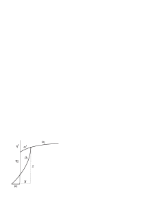
     Figure 5.11. $(\alpha_{1},\beta_{1})+(\mu_{2},\eta_{2})\rightarrow(\alpha^{\prime},\eta^{\prime})$

   • $(\alpha_{1},\beta_{1})+(\mu_{2},\eta_{2})\rightarrow(\alpha^{\prime},\eta^{\prime})$: Figure 5.11
               $A,B\leq 0$ or, $B=-\beta_{1}=-z$ and $A=\alpha^{\prime}-\alpha_{1}\leq y\leq C_{0}z$.

     

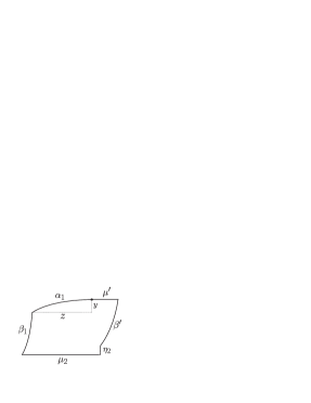
     Figure 5.12. $(\alpha_{1},\beta_{1})+(\mu_{2},\eta_{2})\rightarrow(\mu^{\prime},\beta^{\prime})$

   • $(\alpha_{1},\beta_{1})+(\mu_{2},\eta_{2})\rightarrow(\mu^{\prime},\beta^{\prime})$: Figure 5.12
               $A,B\leq 0$ or; $A=-z$ and $y+\beta_{1}=\beta^{\prime}+\eta_{2}$ $\Rightarrow$ $\beta^{\prime}-\beta_{1}=y-\eta_{2}$ $\Rightarrow$ $B=\beta^{\prime}-\beta_{1}\leq y\leq C_{0}z$.

     

     

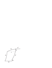
     Figure 5.13. $(\alpha_{1},\beta_{1})+(\mu_{2},\eta_{2})\rightarrow(\alpha^{\prime},\beta^{\prime})$, $0\leq A$ and $0\leq B$.

   • $(\alpha_{1},\beta_{1})+(\mu_{2},\eta_{2})\rightarrow(\alpha^{\prime},\beta^{\prime})$: Figure 5.13
               $B=\beta^{\prime}-\beta_{1}=-z$ and $\alpha_{1}+y=\mu_{2}+\alpha^{\prime}$ $\Rightarrow$ $\alpha^{\prime}-\alpha_{1}=y-\mu_{2}$ $\Rightarrow$ $A=\alpha^{\prime}-\alpha_{1}\leq y\leq C_{0}z$.

   • $(\alpha_{1},\beta_{1})+(\mu_{2},\eta_{2})\rightarrow(\alpha^{\prime},\beta^{\prime})$: Figure 5.13
               $A=\alpha^{\prime}-\alpha_{1}=-z$ and $y+\beta_{1}=\beta^{\prime}+\eta_{2}$ $\Rightarrow$ $\beta^{\prime}-\beta_{1}=y-\eta_{2}$ $\Rightarrow$ $B=\beta^{\prime}-\beta_{1}\leq y\leq C_{0}z$.

5. $(\alpha_{1},\eta_{1})+(\alpha_{2},\beta_{2})$

   

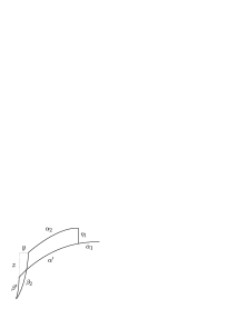
   Figure 5.14. $(\alpha_{1},\eta_{1})+(\alpha_{2},\beta_{2})\rightarrow(\alpha^{\prime},\beta^{\prime})$

   • $(\alpha_{1},\eta_{1})+(\alpha_{2},\beta_{2})\rightarrow(\alpha^{\prime},\beta^{\prime})$: Figure 5.14
               $A=\alpha^{\prime}-\alpha_{1}-\alpha_{2}=y$ and $B=\beta^{\prime}-\beta_{2}=-z$ $\Rightarrow$ $A\leq C_{0}z$.

     

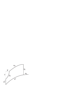
     Figure 5.15. $(\alpha_{1},\eta_{1})+(\alpha_{2},\beta_{2})\rightarrow(\alpha^{\prime},\eta^{\prime})$

   • $(\alpha_{1},\eta_{1})+(\alpha_{2},\beta_{2})\rightarrow(\alpha^{\prime},\eta^{\prime})$: Figure 5.15
               $A=\alpha^{\prime}-\alpha_{1}-\alpha_{2}=y$ and $B=-\beta_{2}=-z$ $\Rightarrow$ $A\leq C_{0}z$.

   

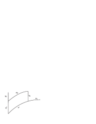
   Figure 5.16. $(\alpha_{1},\eta_{1})+(\alpha_{2},\eta_{2})\rightarrow(\alpha^{\prime},\eta^{\prime})$

6. $(\alpha_{1},\eta_{1})+(\alpha_{2},\eta_{2})\rightarrow(\alpha^{\prime},\eta^{\prime})$: Figure 5.16
             $A=\alpha^{\prime}-\alpha_{1}-\alpha_{2}=0\leq 0$ and $B=0\leq 0$

7. $(\alpha_{1},\eta_{1})+(\mu_{2},\beta_{2})$

   

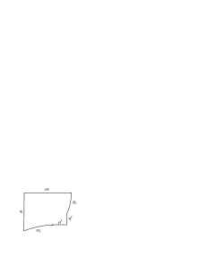
   Figure 5.17. $(\alpha_{1},\eta_{1})+(\mu_{2},\beta_{2})\rightarrow(\mu^{\prime},\eta^{\prime})$

   • $(\alpha_{1},\eta_{1})+(\mu_{2},\beta_{2})\rightarrow(\mu^{\prime},\eta^{\prime})$: Figure 5.17
               $A=-\alpha_{1}\leq 0$ and $B=-\beta_{2}\leq 0.$

     

     

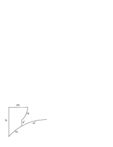
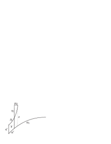
     Figure 5.18. $(\alpha_{1},\eta_{1})+(\mu_{2},\beta_{2})\rightarrow(\alpha^{\prime},\eta^{\prime})$, $A,B\leq 0$ and $0\leq A$.

   • $(\alpha_{1},\eta_{1})+(\mu_{2},\beta_{2})\rightarrow(\alpha^{\prime},\eta^{\prime})$: Figure 5.18
               Either $A\leq 0$ and $B\leq 0$ or $A\leq y$ and $B=-\beta_{2}=z$, therefore, $A\leq-C_{0}B$.

     

     

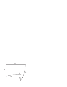
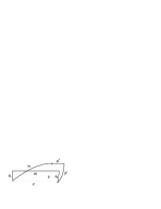
     Figure 5.19. $(\alpha_{1},\eta_{1})+(\mu_{2},\beta_{2})\rightarrow(\mu^{\prime},\beta^{\prime})$, $A,B\leq 0$, and $0\leq B$

   • $(\alpha_{1},\eta_{1})+(\mu_{2},\beta_{2})\rightarrow(\mu^{\prime},\beta^{\prime})$: Figure 5.19
               Either $A\leq 0$ and $B\leq 0$ or $B=\beta^{\prime}-\beta_{2}\leq y$ and $A=-\alpha_{1}=-z$, therefore, $B\leq C_{0}z$.

     

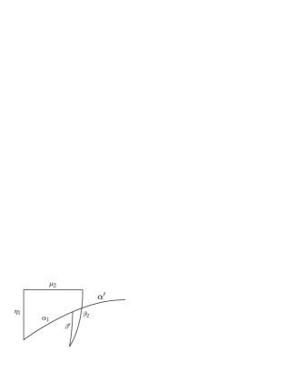
     Figure 5.20. $(\alpha_{1},\eta_{1})+(\mu_{2},\beta_{2})\rightarrow(\alpha^{\prime},\beta^{\prime})$, Case $1$.

     

     

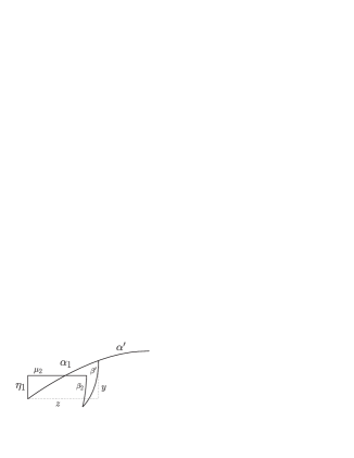
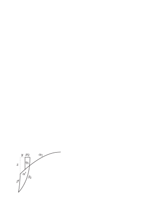
     Figure 5.21. $(\alpha_{1},\eta_{1})+(\mu_{2},\beta_{2})\rightarrow(\alpha^{\prime},\beta^{\prime})$, Case $2$ and $3$.

   • $(\alpha_{1},\eta_{1})+(\mu_{2},\beta_{2})\rightarrow(\alpha^{\prime},\beta^{\prime})$: Figure 5.21 and 5.20
              
     Case $1.)$ $A\leq 0$ and $B\leq 0$.
     Case $2.)$ $A=\alpha^{\prime}-\alpha_{1}=-z$ and $B=\beta^{\prime}-\beta_{1}\leq y\leq C_{0}z$.
     Case $3.)$ $B=\beta^{\prime}-\beta_{2}=-z$ and $A=\alpha^{\prime}-\alpha_{1}=y\leq C_{0}z$.

8. $(\alpha_{1},\eta_{1})+(\mu_{2},\eta_{2})$

   • $(\alpha_{1},\eta_{1})+(\mu_{2},\eta_{2})\rightarrow(\mu^{\prime},\eta^{\prime})$
               $A=-\alpha_{1}\leq 0$ and $B=0\leq 0.$

   • $(\alpha_{1},\eta_{1})+(\mu_{2},\eta_{2})\rightarrow(\alpha^{\prime},\eta^{\prime})$
               $A=-\mu_{2}\leq 0$ and $B=0\leq 0.$

     

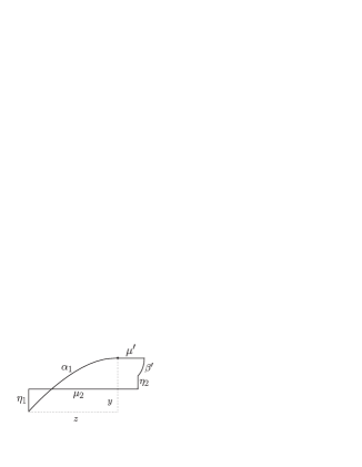
     Figure 5.22. $(\alpha_{1},\eta_{1})+(\mu_{2},\eta_{2})\rightarrow(\mu^{\prime},\beta^{\prime})$

   • $(\alpha_{1},\eta_{1})+(\mu_{2},\eta_{2})\rightarrow(\mu^{\prime},\beta^{\prime})$: Figure 5.22
               $A=-\alpha_{1}=-z$ and $B=\beta^{\prime}\leq y\leq C_{0}z$.

     

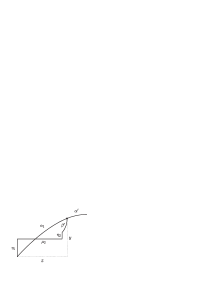
     Figure 5.23. $(\alpha_{1},\eta_{1})+(\mu_{2},\eta_{2})\rightarrow(\alpha^{\prime},\beta^{\prime})$

   • $(\alpha_{1},\eta_{1})+(\mu_{2},\eta_{2})\rightarrow(\alpha^{\prime},\beta^{\prime})$: Figure 5.23
               $A=\alpha^{\prime}-\alpha_{1}=-z$ and $B=\beta^{\prime}\leq y\leq C_{0}z$.

9. $(\mu_{1},\beta_{1})+(\alpha_{2},\beta_{2})$

   

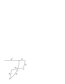
   Figure 5.24. $(\mu_{1},\beta_{1})+(\alpha_{2},\beta_{2})\rightarrow(\mu^{\prime},\beta^{\prime})$

   • $(\mu_{1},\beta_{1})+(\alpha_{2},\beta_{2})\rightarrow(\mu^{\prime},\beta^{\prime})$: Figure 5.24
               $A=-\alpha_{2}=-z$ and $B=y\leq C_{0}z$.

     

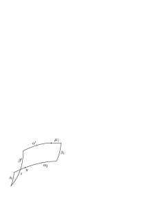
     Figure 5.25. $(\mu_{1},\beta_{1})+(\alpha_{2},\beta_{2})\rightarrow(\alpha^{\prime},\beta^{\prime})$

   • $(\mu_{1},\beta_{1})+(\alpha_{2},\beta_{2})\rightarrow(\alpha^{\prime},\beta^{\prime})$: Figure 5.25
               $A=\alpha^{\prime}-\alpha_{2}=-z$ and $B=\beta^{\prime}-\beta_{1}-\beta_{2}=y\leq C_{0}z$.

   

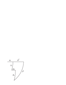
   Figure 5.26. $(\mu_{1},\beta_{1})+(\mu_{2},\beta_{2})\rightarrow(\mu^{\prime},\beta^{\prime})$

10. $(\mu_{1},\beta_{1})+(\mu_{2},\beta_{2})\rightarrow(\mu^{\prime},\beta^{\prime})$: Figure 5.26
              $A=0\leq 0$ and $B=\beta^{\prime}-\beta_{1}-\beta_{2}=0\leq 0$.

11. $(\mu_{1},\beta_{1})+(\alpha_{2},\eta_{2})$

    • $(\mu_{1},\beta_{1})+(\alpha_{2},\eta_{2})\rightarrow(\mu^{\prime},\eta^{\prime})$
                $A=-\alpha_{2}\leq 0$ and $B=-\beta_{1}\leq 0$.

      

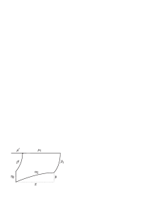
      Figure 5.27. $(\mu_{1},\beta_{1})+(\alpha_{2},\eta_{2})\rightarrow(\mu^{\prime},\beta^{\prime})$

    • $(\mu_{1},\beta_{1})+(\alpha_{2},\eta_{2})\rightarrow(\mu^{\prime},\beta^{\prime})$: Figure 5.27
                $A,B\leq 0$ or, $A=-\alpha_{2}=-z$ and $B=\beta^{\prime}-\beta_{1}\leq y\leq C_{0}z$.

      

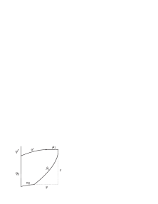
      Figure 5.28. $(\mu_{1},\beta_{1})+(\alpha_{2},\eta_{2})\rightarrow(\alpha^{\prime},\eta^{\prime})$

    • $(\mu_{1},\beta_{1})+(\alpha_{2},\eta_{2})\rightarrow(\alpha^{\prime},\eta^{\prime})$: Figure 5.28
                $A,B\leq 0$ or, we have $y+\alpha_{2}=\mu_{1}+\alpha^{\prime}$. Therefore, with $B=-\beta_{1}=-z$, $A=\alpha^{\prime}-\alpha_{2}=y-\mu_{1}\leq y\leq C_{0}z$.

      

      

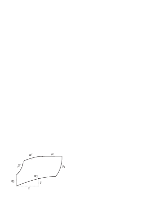
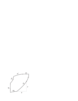
      Figure 5.29. $(\mu_{1},\beta_{1})+(\alpha_{2},\eta_{2})\rightarrow(\alpha^{\prime},\beta^{\prime})$ Case $2$ and $3$.

    • $(\mu_{1},\beta_{1})+(\alpha_{2},\eta_{2})\rightarrow(\alpha^{\prime},\beta^{\prime})$: Figure 5.29
                Case $1.)$ $A\leq 0$ and $B\leq 0$.

                Case $2.)$ $A=\alpha^{\prime}-\alpha_{2}=-z$. Then we know $\beta^{\prime}+\eta_{2}=\beta^{\prime}+y$ and therefore, $B=\beta^{\prime}-\beta_{1}\leq y\leq C_{0}z$.

                Case $3.)$ $B=\beta^{\prime}-\beta_{1}=-z$. Then we know $\alpha^{\prime}+\mu_{1}=\alpha_{2}^{\prime}+y$ and therefore, $A=\alpha^{\prime}-\alpha_{2}\leq y\leq C_{0}z$.

12. $(\mu_{1},\beta_{1})+(\mu_{2},\eta_{2})$

    • $(\mu_{1},\beta_{1})+(\mu_{2},\eta_{2})\rightarrow(\mu^{\prime},\eta^{\prime})$
                $A=0\leq 0$ and $B=-\beta_{1}\leq 0$.

      

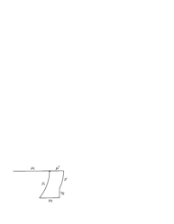
      Figure 5.30. $(\mu_{1},\beta_{1})+(\mu_{2},\eta_{2})\rightarrow(\mu^{\prime},\beta^{\prime})$

    • $(\mu_{1},\beta_{1})+(\mu_{2},\eta_{2})\rightarrow(\mu^{\prime},\beta^{\prime})$: Figure 5.30
                $A=0$ and $B=\beta^{\prime}-\beta_{2}\leq 0$.

      

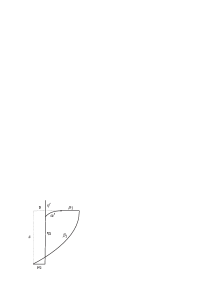
      Figure 5.31. $(\mu_{1},\beta_{1})+(\mu_{2},\eta_{2})\rightarrow(\alpha^{\prime},\eta^{\prime})$

    • $(\mu_{1},\beta_{1})+(\mu_{2},\eta_{2})\rightarrow(\alpha^{\prime},\eta^{\prime})$: Figure 5.31
                $B=-\beta_{1}=-z$ and $A=\alpha^{\prime}\leq y\leq C_{0}z$.

      

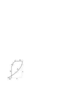
      Figure 5.32. $(\mu_{1},\beta_{1})+(\mu_{2},\eta_{2})\rightarrow(\alpha^{\prime},\beta^{\prime})$

    • $(\mu_{1},\beta_{1})+(\mu_{2},\eta_{2})\rightarrow(\alpha^{\prime},\beta^{\prime})$: Figure 5.32
                We have $B=\beta^{\prime}-\beta_{1}=-z$ and $y=\alpha^{\prime}+\mu_{1}+\mu_{2}$. Thus, $A=\alpha^{\prime}\leq y\leq C_{0}z$.

13. $(\mu_{1},\eta_{1})+(\alpha_{2},\beta_{2})$

    

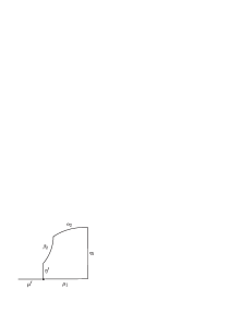
    Figure 5.33. $(\mu_{1},\eta_{1})+(\alpha_{2},\beta_{2})\rightarrow(\mu^{\prime},\eta^{\prime})$

    • $(\mu_{1},\eta_{1})+(\alpha_{2},\beta_{2})\rightarrow(\mu^{\prime},\eta^{\prime})$: Figure 5.33
                We have $A=-\alpha_{2}\leq 0$ and $B=-\beta_{2}\leq 0$.

      

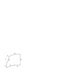
      Figure 5.34. $(\mu_{1},\eta_{1})+(\alpha_{2},\beta_{2})\rightarrow(\alpha^{\prime},\eta^{\prime})$

    • $(\mu_{1},\eta_{1})+(\alpha_{2},\beta_{2})\rightarrow(\alpha^{\prime},\eta^{\prime})$: Figure 5.34
                $B=-\beta_{2}=-z\leq 0$ and $A=\alpha^{\prime}-\alpha_{2}=y-\mu_{1}\leq y\leq C_{0}z$.

      

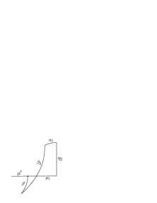
      Figure 5.35. $(\mu_{1},\eta_{1})+(\alpha_{2},\beta_{2})\rightarrow(\mu^{\prime},\beta^{\prime})$

    • $(\mu_{1},\eta_{1})+(\alpha_{2},\beta_{2})\rightarrow(\mu^{\prime},\beta^{\prime})$: Figure 5.35
                $A=-\alpha_{2}\leq 0$, $B=\beta^{\prime}-\beta_{2}\leq-\eta_{2}\leq 0$.

      

      

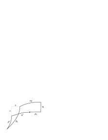
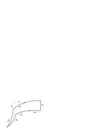
      Figure 5.36. $(\mu_{1},\eta_{1})+(\alpha_{2},\beta_{2})\rightarrow(\alpha^{\prime},\beta^{\prime})$ Case $1$ and $2$.

    • $(\mu_{1},\eta_{1})+(\alpha_{2},\beta_{2})\rightarrow(\alpha^{\prime},\beta^{\prime})$: Figure 5.36
                Case $1.)$ $B=\beta^{\prime}-\beta_{2}=-z$. Since $\alpha_{2}+y=\mu_{1}+\alpha^{\prime}$, we have $A=\alpha^{\prime}-\alpha_{2}=y-\mu_{1}$. Therefore, $A=\alpha^{\prime}-\alpha_{2}\leq y\leq C_{0}z$.
      

                Case $2.)$ $A=\alpha^{\prime}-\alpha_{2}=-z$. Since $\beta_{2}+y=\beta^{\prime}+\eta_{1}$, we have $B=\beta^{\prime}-\beta_{2}\leq y\leq C_{0}z$.

14. $(\mu_{1},\eta_{1})+(\mu_{2},\beta_{2})$

    

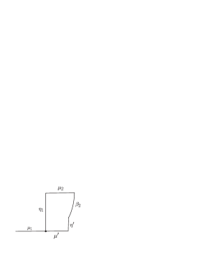
    Figure 5.37. $(\mu_{1},\eta_{1})+(\mu_{2},\beta_{2})\rightarrow(\mu^{\prime},\eta^{\prime})$

    • $(\mu_{1},\eta_{1})+(\mu_{2},\beta_{2})\rightarrow(\mu^{\prime},\eta^{\prime})$: Figure 5.37
                We have $A=0\leq 0$ and $B=-\beta_{2}\leq 0$.

      

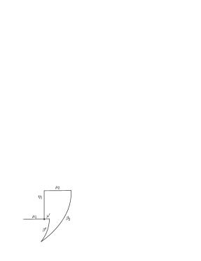
      Figure 5.38. $(\mu_{1},\eta_{1})+(\mu_{2},\beta_{2})\rightarrow(\mu^{\prime},\beta^{\prime})$

    • $(\mu_{1},\eta_{1})+(\mu_{2},\beta_{2})\rightarrow(\mu^{\prime},\beta^{\prime})$: Figure 5.38
                $A=0\leq 0$ and $B=\beta^{\prime}-\beta_{2}=-\eta_{1}\leq 0$.

      

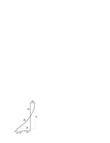
      Figure 5.39. $(\mu_{1},\eta_{1})+(\mu_{2},\beta_{2})\rightarrow(\alpha^{\prime},\eta^{\prime})$

    • $(\mu_{1},\eta_{1})+(\mu_{2},\beta_{2})\rightarrow(\alpha^{\prime},\eta^{\prime})$: Figure 5.39
                $B=-\beta_{2}=-z$ and $A=\alpha^{\prime}\leq y\leq C_{0}z$.

      

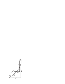
      Figure 5.40. $(\mu_{1},\eta_{1})+(\mu_{2},\beta_{2})\rightarrow(\alpha^{\prime},\beta^{\prime})$

    • $(\mu_{1},\eta_{1})+(\mu_{2},\beta_{2})\rightarrow(\alpha^{\prime},\beta^{\prime})$: Figure 5.40
                $B=\beta^{\prime}-\beta_{2}=-z$ and $A=\alpha^{\prime}\leq y\leq C_{0}z$.

15. $(\mu_{1},\eta_{1})+(\mu_{2},\eta_{2})$

    

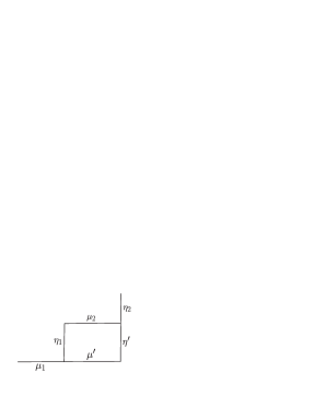
    Figure 5.41. $(\mu_{1},\eta_{1})+(\mu_{2},\eta_{2})\rightarrow(\mu^{\prime},\eta^{\prime})$

    • $(\mu_{1},\eta_{1})+(\mu_{2},\eta_{2})\rightarrow(\mu^{\prime},\eta^{\prime})$: Figure 5.41
                We have $A=0\leq 0$ and $B=0\leq 0$.

16. $(\mu_{1},\eta_{1})+(\alpha_{2},\eta_{2})$

    

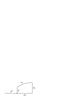
    Figure 5.42. $(\mu_{1},\eta_{1})+(\alpha_{2},\eta_{2})\rightarrow(\mu^{\prime},\eta^{\prime})$

    • $(\mu_{1},\eta_{1})+(\alpha_{2},\eta_{2})\rightarrow(\mu^{\prime},\eta^{\prime})$: Figure 5.42
                We have $A=-\alpha_{1}\leq 0$ and $B=0\leq 0$.

      

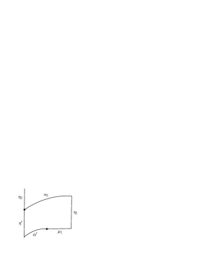
      Figure 5.43. $(\mu_{1},\eta_{1})+(\alpha_{2},\eta_{2})\rightarrow(\alpha^{\prime},\eta^{\prime})$

    • $(\mu_{1},\eta_{1})+(\alpha_{2},\eta_{2})\rightarrow(\alpha^{\prime},\eta^{\prime})$: Figure 5.43
                We have $A=\alpha^{\prime}-\alpha_{2}=-\mu_{1}\leq 0$ and $B=0\leq 0$.

      

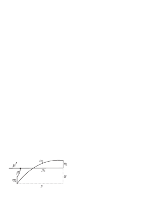
      Figure 5.44. $(\mu_{1},\eta_{1})+(\alpha_{2},\eta_{2})\rightarrow(\mu^{\prime},\beta^{\prime})$

    • $(\mu_{1},\eta_{1})+(\alpha_{2},\eta_{2})\rightarrow(\mu^{\prime},\beta^{\prime})$: Figure 5.44
                We have $A=-\alpha_{2}=-z$ and $B\leq y\leq C_{0}z$.

      

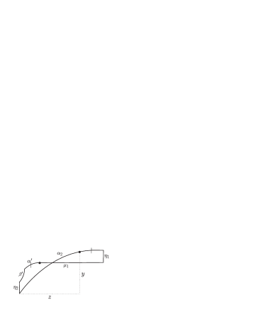
      Figure 5.45. $(\mu_{1},\eta_{1})+(\alpha_{2},\eta_{2})\rightarrow(\alpha^{\prime},\beta^{\prime})$

    • $(\mu_{1},\eta_{1})+(\alpha_{2},\eta_{2})\rightarrow(\alpha^{\prime},\beta^{\prime})$: Figure 5.45
                We have $A=\alpha^{\prime}-\alpha_{2}=-z$ and $B=\beta^{\prime}\leq y\leq C_{0}z$.

Bibliography

- [1] Anile, A.M., Relativistic Fluids and Magneto-Fluids, Cambridge University Press, .
- [2] Bressan, A., Hyperbolic Systems of Conservation Laws: The One-Dimensional Cauchy Problem, Oxford University Press, .
- [3] Courant, R., Friedrichs, K.O., Supersonic Flow and Shock Waves, Springer-Verlag, New York, .
- [4] Glimm, J., Solutions in the large for nonlinear hyperbolic systems of equations, Comm. Pure. Appl. Math , , p
- [5] Lax, P.D., Hyperbolic systems of conservation laws, II, Comm. Pure Appl. Math., , p.
- [6] Liu, T. P., Solutions in the Large for the Equations of Nonisentropic Gas Dynamics, Ind. Univ. Math. J., Vol. , No.1 .
- [7] Misner, C.W., Thorne, K.S. and Wheeler, J.A., Gravitation, W.H. Freeman and Company, New York, .
- [8] Nishida, T., Smoller, J., Solutions in the Large for Some Nonlinear Hyperbolic Conservation Laws. Comm. Pure Appl. Math. , , p.
- [9] Smoller, J., Shock Waves and Reaction Diffusion Equations, Springer N.Y., .
- [10] Smoller, J. and Temple, B., Global Solutions of the Relativistic Euler Equations, Commun. Math. Phys. , , p.
- [11] Taub, A. H., Relativistic Rankine-Hugonoit Equations, Phys. Rev., Vol 74, No. , , p.
- [12] Temple, B., Solutions in the large for the nonlinear hyperbolic conservation laws of gas dynamics, J. Differential Equations, , no. , .
- [13] Wald, R.M., General Relativity, The University of Chicago Press, Chicago and London, .
- [14] Weinberg, S., Gravitation and Cosmology: Principles and Applications of the General Theory of Relativity, New York, Wiley, .