Galaxy clustering constraints on deviations from Newtonian gravity at cosmological scales II: Perturbative and numerical analyses of power spectrum and bispectrum
Abstract
We explore observational constraints on possible deviations from Newtonian gravity by means of large-scale clustering of galaxies. We measure the power spectrum and the bispectrum of Sloan Digital Sky Survey galaxies and compare the result with predictions in an empirical model of modified gravity. Our model assumes an additional Yukawa-like term with two parameters that characterize the amplitude and the length scale of the modified gravity. The model predictions are calculated using two methods; the second-order perturbation theory and direct -body simulations. These methods allow us to study non-linear evolution of large-scale structure. Using the simulation results, we find that perturbation theory provides reliable estimates for the power spectrum and the bispectrum in the modified Newtonian model. We also construct mock galaxy catalogues from the simulations, and derive constraints on the amplitude and the length scale of deviations from Newtonian gravity. The resulting constraints from power spectrum are consistent with those obtained in our earlier work, indicating the validity of the previous empirical modeling of gravitational nonlinearity in the modified Newtonian model. If linear biasing is adopted, the bispectrum of the SDSS galaxies yields constraints very similar to those from the power spectrum. If we allow for the nonlinear biasing instead, we find that the ratio of the quadratic to linear biasing coefficients, , should satisfy in the modified Newtonian model.
pacs:
04.50.+h 98.65.-r 98.80.EsI Introduction
Recent measurements of cosmic microwave background radiation angular power spectrum Spergel:2006hy ; Bennett:2003bz ; Spergel:2003cb strongly support the “standard” cosmological model in which the energy content of the universe is dominated by dark energy (very close to Einstein’s cosmological constant, ) and cold dark matter (CDM). Such CDM universes are also in good agreement with independent datasets of galaxy clustering Tegmark:2004uf ; Cole:2005sx and distant Type Ia supernovae Knop:2003iy ; Astier:2006pq ; Riess:2007rs . Thus the basic framework for the theory of structure formation in the universe is firmly established. Nevertheless the nature and the physical origin of dark energy remain to be understood.
The apparent accelerating expansion of the universe is conventionally interpreted in terms of a source of repulsive force (dark energy), but can be explained by modifying Newton’s law of gravity on cosmological scales as well. The latter resolution has been seriously considered recently. For example, Dvali, Gabadadze and Porrati (DGP) Dvali:2000hr ; Deffayet:2000uy propose that gravity leaking into extra dimensions drives the observed accelerating expansion. Other such models include modified Newtonian dynamics (MOND) Sanders:2002pf ; Scarpa:2006cm ; Bekenstein:2004ne and ghost condensation Arkani-Hamed:2003uy ; Arkani-Hamed:2003uz . Intriguingly, all of these alternative models predict some deviation from conventional Newtonian gravity at cosmological scales.
Indeed, while the validity of Newtonian gravity is tested to high precision up to the scale of the solar system ( m), there have been no rigorous tests at sub-millimeter and over scales beyond the solar system Fischbach:1999bc ; Adelberger:2003zx ; Hoyle:2004cw . It has been suggested that large-scale galaxy clustering can be used to constrain non-Newtonian models of gravity Frieman:1991 in principle, but it became feasible only recently with accurate measurements of galaxy clustering in large redshift surveys Tegmark:2004uf ; Cole:2005sx .
In our earlier work Shirata:2005yr (Paper I), we put quantitative constraints on deviations from Newtonian gravity at cosmological scales under the assumption that the deviation can be described in a simple parametric form; we adopted an empirical Yukawa-like term for the modified gravity, and calculated the galaxy-galaxy power spectrum semi-analytically. (See also Ref. Sealfon:2004gz for similar argument.) By comparing the predicted power spectrum with that of SDSS galaxies Tegmark:2004uf , we derived quantitative, although still conditional, constraints on deviations from Newton’s law of gravity.
In this paper, we improve our previous work by performing non-linear cosmological simulations and by exploiting a higher-order statistic, bispectrum. Since bispectrum is sensitive to clustering in the non-linear regime, it is expected to provide complementary constraints at mega-parsec scales to that obtained from power spectrum analysis. We use direct -body simulations to test the accuracy of our semi-analytic calculations and to reinforce our conclusions.
The rest of the paper is organized as follows. Our model assumptions are described in Sec. II. We derive power spectrum and bispectrum from perturbation theory in modified Newtonian model in Sec. III and IV. We perform -body simulations and construct mock samples of volume-limited SDSS galaxies for direct comparison with the observational data. Details of the simulations are described in Sec. V. The results of perturbation theory and the simulations are discussed in Sec. VI and VII. Finally Sec. VIII concludes the present analysis.
II Model Assumptions
In this section, we briefly summarize our model and a set of assumptions. Further details may be found in Paper I.
We consider a modified Newtonian model for which gravitational potential is given by
| (1) |
where denotes (conventional) Newton’s constant of gravity. The above model corresponds to Model II in Paper I, on which we focus throughout the following analysis. The deviation from the Newtonian gravity in this model is characterized by two parameters, and ; is the dimensionless amplitude of the deviation and is the characteristic length scale. Note that is defined in the proper length, rather than in the comoving length.
It is important to note that, although we consider deviations from Newtonian gravity at mega-parsec scales, we still assume that the global cosmic expansion is unaffected by the deviations. Namely, we assume that general relativity is valid on horizon scales and thus the cosmic expansion is described by the standard Friedmann equation. Strictly speaking, these two assumptions may be in conflict with modified gravity models in general Deffayet:2001pu ; Lue:2004rj ; Alcaniz:2004kq ; Lue:2004za ; Yamamoto:2006yv . To account for the existing data such as SNeIa and CMB, however, the cosmic expansion law can hardly change in practice. This is why we adopt the conventional Friedmann equation even in this analysis. For the same reason, we use conventional matter transfer function as initial condition of dark matter adopting the background cosmology defined by the standard set of cosmological parameters, =0.3, =0.04, , and the Hubble constant at present in units of 100km Mpc-1. See Paper I for further discussion on this point.
In order to make a direct comparison between the clustering of SDSS galaxies and our model predictions, we need to assume a biasing relation for the distribution of galaxies and that of matter. For this purpose, we adopt a commonly adopted deterministic relation:
| (2) |
where and are fractional fluctuation of galaxy number and mass density, and are linear and quadratic biasing parameters. We consider only linear bias (i.e., ) when we use power spectrum, whereas we consider both and for analyses using bispectrum. To derive constraints on and , is treated as a free parameter to adjust the overall clustering amplitude.
III Power spectrum analysis
In Fourier space, the modified gravitational potential in Eq. (1) can be written as
| (3) |
where is in the comoving coordinate, is the comoving wave-number, and is the scale factor normalized unity at the present epoch.
For the potential of Eq. (3), the evolution equation for density perturbations is written as
| (4) |
with
| (5) | |||
| (6) |
where is the Hubble parameter, and denotes the linear term in density fluctuations [see Eq. (16) below]. Note that even the linear perturbation equation becomes dependent on in the modified gravity model.
Next, the linear power spectrum at present is given by
| (7) |
where is the matter transfer function, and is the spectral index of the primordial power spectrum which we set to be unity. We use the fitting formula of Eisenstein and Hu Eisenstein:1997ik for . It should be emphasized here that we fix the amplitude so that the rms value of the top-hat mass fluctuations at 8Mpc, , equals 0.9 when and . The actual value of in our modified gravity model may be slightly different because of the factor in Eq. (7). However, the difference in the overall amplitude is unimportant because we have an additional freedom to adjust the predicted amplitude via the biasing relation [Eq. (2)].
In Paper I we used the Peacock-Dodds prescription Peacock:1996ci to convert the linear power spectrum to nonlinear one. It turned out that in doing so we used incorrectly the growth factor and the tilt of linear power spectrum given in the case of Newtonian models. We made sure later that the above mistake did not change the final power spectra very much as long as the Peacock-Dodds prescription is valid. In the present paper, we also confirm the validity of the Peacock-Dodds approach in non-Newtonian models using -body simulations directly (see Sec. VI).
IV Perturbation theory and bispectrum
In this section, we describe the second order perturbation theory and its application to bispectrum. The earlier formulation of cosmological perturbation in the Newtonian model may be found in Juszkiewicz:1981 ; Vishniac:1983 ; Suto:1990wf ; Makino:1991rp . Bernardeau Bernardeau:2004ar developed a formulation of second order perturbation theory in non-Newtonian models. We apply the method to the modified potential in Eq. (1).
The basic equations are given by
| (8) | |||
| (9) |
where the over-dot denotes the derivative with respect to time, is the peculiar velocity, and is the gravitational potential. We define velocity divergence:
| (10) |
These equations can be solved recursively. Let us first decompose and perturbatively,
| (16) | |||
| (17) |
Differentiating Eq. (11) and substituting to Eq. (14) to eliminate , we obtain
| (18) |
where and are the source terms of the th-order:
| (19) | |||
| (20) |
Consider first the lowest order, . Since , Eq. (18) reduces to
| (21) |
which is equivalent to Eq. (4). We denote the growing mode of the solution of Eq. (21) by . Note that, in non-Newtonian models, the solution is generally dependent on scale , in contrast to the conventional Newtonian case. The linear solution is given by
| (22) |
where is the initial fractional density.
The corresponding linear solution for is obtained from Eq. (11) as
| (23) |
Solutions at the next order, , are more complicated. Eq. (18) for is written explicitly as
| (24) | |||
| (25) | |||
| (26) | |||
| (27) |
where is the Delta function and are the Legendre polynomials:
| (28) | |||
| (29) |
Equation (24) has an implicit solution of the form:
| (30) |
where the functions satisfy
| (31) |
We note that expressions for the second-order solutions given in Bernardeau:2004ar contain some typographical errors which are corrected in our above expressions.
These results enable us to compute the bispectrum in the leading order. The bispectrum is defined as
| (32) |
The leading-order terms of the left-hand-side of the above equation are given by
| (33) |
Therefore the bispectrum reduces to
| (34) |
where . In what follows, we write the bispectrum simply as adopting the condition of [Eq. (32)].
V Simulation and observational data
V.1 N-body Simulations
We use the cosmological -body solver TPM-1.1 Bode:2003ct in its PM-only mode. We run six realizations each for simulation box-sizes of Mpc, and Mpc with the following parameters: and , and Mpc. We use the fitting formula for the matter transfer function, equation (28) (31) of the ref. Eisenstein:1997ik , that ignores the baryon acoustic oscillation effect. We start the simulations at . All the simulations employ particles.
To simulate structure formation in the non-Newtonian model, we need to modify the Green function of the Laplacian, . For a density field defined on a three-dimensional wave-number grid , the gravitational potential in real space is evaluated to be
| (38) |
where are position integers in real space with being the number of grids per dimension (we follow the notation in Efstathiou et al. Efstathiou:1985re ).
The Green function in the original TPM code that assumes the conventional Newtonian gravity is given by
| (39) |
which is derived from the seven-point finite-difference approximation.
Taking account of the scale-dependence in Eq. (3), we correct the Green function for the modified Newtonian model:
| (40) |
Note that in Eq. (40) needs to be given in the form, consistently with the Green function itself, as
| (41) |
We use the above Green function, evolve the system from to , and make mock galaxy samples in the manner described in the next subsection.
|
|
|
|
|
|
V.2 Observational data and mock samples
For definiteness, we choose a volume-limited sample of SDSS galaxies whose -band magnitude is in the range of (-21.0, -20.0) from those described in Hikage et al. Hikage:2005ia . The redshift range is , the survey volume, , is , and the total number of galaxies is 44,636. We made sure that using the other volume-limited samples with different magnitude ranges Hikage:2005ia does not significantly affect the results of our analysis below.
We generate 24 mock catalogues from our -body simulation data. The mock catalogues take into account various observational effects such as survey geometry, the number density, and redshift distortion (peculiar velocities of simulations particles are assigned to the mock galaxies ) Hikage:2005ia . In order to account for the effect of survey geometry, we distribute random particles within the survey volume and correct for the boundary effect following the prescription of Feldman, Kaiser and Peacock FKP . We subtract fluctuations of the random particles which are within the survey volume, :
| (42) |
While this prescription is fairly empirical and may not completely account for the effect of the survey geometry, it yields a robust estimate at scales of our main interest here, . When we calculate the power spectrum and bispectrum for SDSS galaxies and the mock catalogues, we use the above “corrected” density, .
VI Constraints from power spectrum
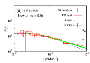
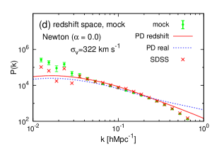
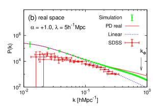
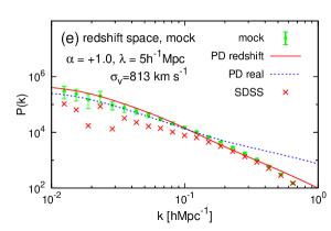
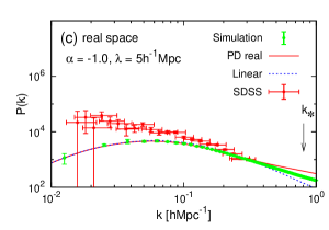
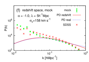
We first compare the power spectra used the Peacock-Dodds prescription and those from numerical simulations. In Fig. 1, we plot the mass power spectra in real space (left panels) and in redshift space (right panels). The predictions from perturbation theory agree well with the results of -body simulations.. Note that in the Newtonian case, the predicted power spectra with are already in reasonable agreement with the observed power spectrum of SDSS galaxies. Our simulation results are also consistent with those of Stabenau and Jain Stabenau:2006td .
The panels on the right side in Fig. 1 show the power spectra of our mock “galaxies”. In each panel, the dotted line indicates the non-linear power spectrum in real space, which is the same in the corresponding left panel and shown for comparison. The redshift-space power spectrum of the SDSS volume-limited sample is shown by cross symbols. To include effects of redshift space distortion in our model, we use the formula derived of Magira, Jing and Suto Magira:1999bn [equation (12) in their paper]. On linear scales (Mpc-1), the Kaiser effect is clearly seen as an enhanced power with respect to the real space power spectrum. It is worth mentioning that the plotted power spectra show substantial variations on the largest scales (), which are presumably due to the somewhat complex survey geometry.
|
|
|
To derive constraints on using the calculated power spectra, we apply the statistic. We treat the linear bias parameter as a free parameter in order to adjust the overall amplitudes of the power spectra between the predictions/simulations and the SDSS data. This normalization allows us to use the shape of the power spectra to detect possible deviations from the Newtonian case.
We calculate as
| (43) |
where is the SDSS galaxy power spectrum. We use the predicted power spectra and the variance of the SDSS data, , to calculate in real space, while for the same analysis in redshift space, we use those power spectra with the variance of mock galaxy samples to represent the cosmic variance in redshift space.
We compute the relative confidence level of and with respect to their best-fit values assuming that
| (44) |
follows the distribution for 2 degrees of freedom. In Eq. (44), , and denote their best-fit values which globally minimize the value of , while is the value that minimizes the for a given set of values of and .
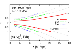
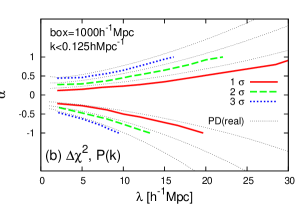
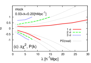
Figure 2 shows the contours of . The results from -body simulations in real space are shown in panel (a) and (b). These differ only in the simulation box size, 500 Mpc for (a) and 1000 Mpc for (b). Hence the range of used to derive constraints is slightly different, We also show the result from the real-space Peacock-Dodds prediction by thin dotted lines using the the same range of consistently with the simulations. Clearly, the results of the perturbation theory and that of our numerical simulations are consistent with each other, putting quite similar constraints on and .
The bottom panel (c) in Figure 2 shows the constraints from our mock galaxy samples in redshift space. The range of used in the analysis is Mpc-1. The constraint is slightly less tight than those from perturbation theory and -body simulations. This is mainly because we discard the data points at large scales Mpc-1 where the deviations from the Newtonian case are most significant. Nevertheless models with are still excluded at a 2-3 confidence level for . For reference, we also plot the contours based on the real-space Peacock-Dodds prediction by thin dotted lines.
VII Constraints from bispectrum
We further derive constraints on the modified Newtonian model extending the analysis to the three-point statistics. Specifically we use (conventional) bispectrum, , defined in Eq. (32), and reduced bispectra and defined as
| (45) |
and
| (46) |
where , , and is the sampling volume. The latter quantity is the probability density function of phase sum for a density field, [], studied in Matsubara Matsubara:2003te and Hikage et al. Hikage:2003kr ; Hikage:2005ia . In this paper, we consider only isosceles triangles in -space that satisfy the relation with angle defined as
| (47) |
In the following analysis, we use to give constraints on the deviation from Newtonian gravity. This is because consists only of Fourier-phase informations and thus their constraints have good complementarity with those from , which is defined as the square of the Fourier amplitudes.
|
|
|
|
|
|
|
|
|
|
|
|
|
|
|
VII.1 Linear bias model with
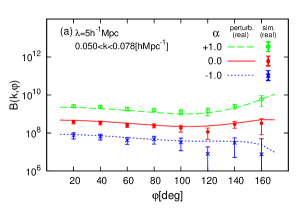
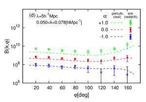
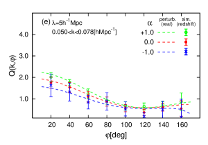
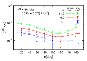
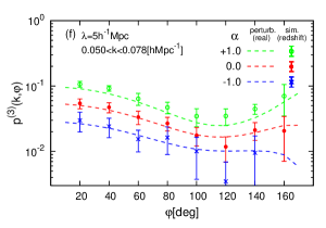
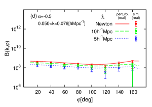
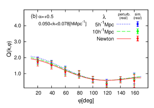
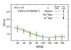
Let us consider first linear bias model [ in Eq. (2)]. Figure 3 plots the bispectra in real space (left panels) and in redshift space (right panels) for 500 Mpc simulations. The survey volume is set to be in Eq. (46). The bispectra at small are dominated by various nonlinear effects, whereas there are substantial uncertainties at large because of the small number of Fourier modes sampled. Given those, the agreement between predictions from perturbation theory (dashed lines) and -body simulation data (solid circles with error-bar) is very satisfactory.
The right panels of Fig. 3 shows the bispectra in redshift space. There, the results from our mock samples are shown by symbols with error bars. For comparison, we also show the results from perturbation theory in real space. In Fig. 3(d), Kaiser effect is clearly seen as a enhance at small .
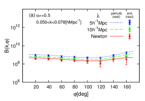
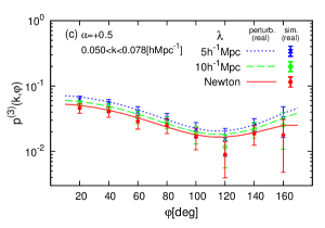
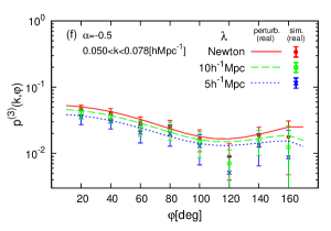
We further examine the dependence of the bispectra on . Figure 4 compares the bispectra for different values of . We have set = 0.5 (left panels) and (right panels).
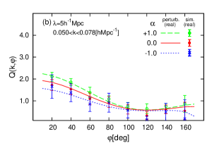
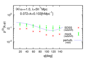
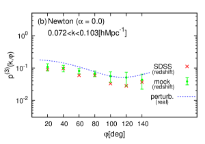
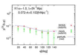
Figure 5 shows for the volume-limited SDSS catalogue and for our mock samples at in the range of . They have a very similar shape, but their amplitude depends systematically on the value of , the degree of deviations from the Newtonian case.
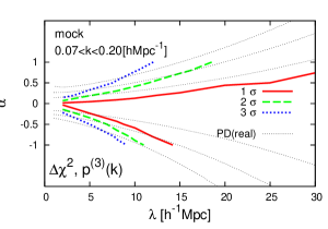
Figure 6 plots constraints on the plane derived from the fit to the SDSS bispectrum using and assuming a linear bias (). The constraints from the bispectrum are fairly consistent with, but slightly more stringent than, those from the power spectrum, which indicates the complementary role of the higher-order clustering statistics.
|
|
|
VII.2 The effect of non-linear biasing
In reality, however, it may be more appropriate to analyze the higher-order clustering statistics adopting a nonlinear bias model. In the case of the bispectrum, it implies to introduce the quadratic biasing parameter [see Eq. (2)]. In this bias model, the relation of for galaxies and for mass reduces to
| (48) | |||
| (49) |
where for Hikage:2005ia .
Previous papers Hikage:2005ia ; Nishimichi:2006 suggest that a simple linear bias model in the Newtonian gravity model describes well the clustering of the volume-limited sample of SDSS galaxies, i.e., and . We now repeat the similar analysis in the modified Newtonian model.
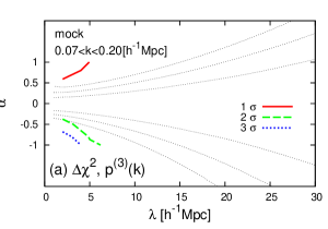
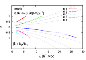
Figure 7(a) indicates constraints on the plane by treating as a free parameter, which should be compared with Figure 6 for . The regions below the contours are excluded with the corresponding confidence level. Naturally the bispectrum alone does not constrain significantly in this generalized model. While the models are excluded with a 1 confidence level, the conclusion is not statistically significant. In turn, however, we can derive constraints on the value of for the modified gravity model by combining the constraints from power spectrum (independent of the value of ). Figure 7(b) shows the contours of the best-fit value of that gives the minimum for on the plane. Figure 7(b) suggests that should satisfy , which is the first constraint on the quadratic biasing parameter in the modified Newtonian model.
VIII Summary
We have derived constraints on possible deviations from Newtonian gravity using the power spectrum and the bispectrum of Sloan Digital Sky Survey galaxies. Our model assumes an additional Yukawa-like term with two parameters that characterize the amplitude, , and the length scale, , of the modified gravity. We have predicted the power spectrum and the bispectrum using two different methods, the perturbation theory and direct -body simulations, and found the good agreement in real space as long as the biasing between galaxies and mass is neglected. In order to take the biasing effect into consideration, we adopt a quadratic biasing model. By comparing with the mock catalogues constructed from our simulations, we have derived constraints on and . This method allows us to compute the clustering statistics in redshift space and taking account of various observational effects such as survey geometry as well. The resulting constraints from power spectrum are consistent with those obtained in our earlier work, indicating the validity of the previous empirical modeling of gravitational nonlinearity in the modified Newtonian model. If linear biasing is adopted, the bispectrum of the SDSS galaxies yields constraints very similar to those from the power spectrum. If we allow for the nonlinear biasing instead, we find that the ratio of the quadratic to linear biasing coefficients, , should satisfy . in the modified Newtonian model.
Future observations will exploit large ground-based telescopes to probe the matter density distribution by weak gravitational lensing. Combined with data from galaxy redshift surveys, lensing observations will provide invaluable informations on galaxy bias. Then it will be possible to put more stringent constraints on deviations from Newton’s law of gravity at cosmological scales, using the methodology presented in the this paper.
Acknowledgements
We would like to thank Atsushi Taruya, Kazuhiro Yahata, Takahiro Nishimichi, Shun Saito, and Issya Kayo for useful discussions and comments. A. S. acknowledge the support from Grants-in-Aid for Japan Society for the Promotion of Science Fellows. The simulations were performed at the Data-Reservoir at the University of Tokyo. We thank Mary Inaba and Kei Hiraki at the University of Tokyo for providing the computational resources. This work is supported in part by Grants-in-Aid for Scientific research of the Ministry of Education, Culture, Sports, Science and Technology (No. 17684008, and 18072002), and by JSPS (Japan Society for Promotion of Science) Core-to-Core Program “International Research Network for Dark Energy”.
References
- (1) D. N. Spergel et al., astro-ph/0603449.
- (2) C. L. Bennett et al., Astrophys. J. Suppl. 148, 1 (2003)
- (3) D. N. Spergel et al. Astrophys. J. Suppl. 148, 175 (2003)
- (4) M. Tegmark et al. Astrophys. J. 606, 702 (2004)
- (5) S. Cole et al. Mon. Not. Roy. Astron. Soc. 362, 505 (2005)
- (6) R. A. Knop et al., Astrophys. J. 598, 102 (2003)
- (7) P. Astier et al., A& A, 447, 31 (2006)
- (8) A. G. Riess et al., astro-ph/0611572
- (9) G. R. Dvali, G. Gabadadze and M. Porrati, Phys. Lett. B 485, 208 (2000)
- (10) C. Deffayet, Phys. Lett. B 502, 199 (2001)
- (11) R. H. Sanders and S. S. McGaugh, Ann. Rev. Astron. Astrophys. 40, 263 (2002)
- (12) R. Scarpa, in AIP Conference Proceedings, Vol 822, 2006, edited by E.J Lerner and J.B. Almeida, p. 253.
- (13) J. D. Bekenstein, Phys. Rev. D 70, 083509 (2004); D 71, 069901(E) (2005)
- (14) N. Arkani-Hamed, H. C. Cheng, M. A. Luty and S. Mukohyama, JHEP 0405, 074 (2004)
- (15) N. Arkani-Hamed, P. Creminelli, S. Mukohyama and M. Zaldarriaga, JCAP 0404, 001 (2004)
- (16) E. Fischbach and C. L. Talmadge, The search for non-Newtonian gravity (Springer, New York, 1999)
- (17) E. G. Adelberger, B. R. Heckel and A. E. Nelson, Ann. Rev. Nucl. Part. Sci. 53, 77 (2003)
- (18) C. D. Hoyle, D. J. Kapner, B. R. Heckel, E. G. Adelberger, J. H. Gundlach, U. Schmidt and H. E. Swanson, Phys. Rev. D 70, 042004 (2004)
- (19) J. A. Frieman and B. Gradwohl, Phys. Rev. Lett. 67, 2926 (1991).
- (20) A. Shirata, T. Shiromizu, N. Yoshida and Y. Suto, Phys. Rev. D 71, 064030 (2005)
- (21) C. Sealfon, L. Verde and R. Jimenez, Phys. Rev. D 71, 083004 (2005)
- (22) C. Deffayet, G. R. Dvali and G. Gabadadze, Phys. Rev. D 65, 044023 (2002)
- (23) A. Lue, R. Scoccimarro and G. D. Starkman, Phys. Rev. D 69, 124015 (2004)
- (24) J. S. Alcaniz and N. Pires, Phys. Rev. D 70, 047303 (2004)
- (25) A. Lue and G. D. Starkman, Phys. Rev. D 70, 101501 (2004)
- (26) K. Yamamoto, B. A. Bassett, R. C. Nichol, Y. Suto and K. Yahata, Phys. Rev. D 74,063525 (2006)
- (27) D. J. Eisenstein and W. Hu, Astrophys. J. 496, 605 (1998)
- (28) J. A. Peacock and S. J. Dodds, Mon. Not. Roy. Astron. Soc. 280, L19 (1996)
- (29) R. Juszkiewicz, Mon. Not. Roy. Astron. Soc. 197, 931 (1981)
- (30) E. T. Vishniac Mon. Not. Roy. Astron. Soc. 203, 345 (1983)
- (31) Y. Suto and M. Sasaki, Phys. Rev. Lett. 66, 264 (1991).
- (32) N. Makino, M. Sasaki and Y. Suto, Phys. Rev. D 46, 585 (1992).
- (33) F. Bernardeau, arXiv:astro-ph/0409224.
- (34) P. Bode and J. P. Ostriker, Astrophys. J. Suppl. 145, 1 (2003)
- (35) G. Efstathiou, M. Davis, C. S. Frenk and S. D. M. White, Astrophys. J. Suppl. 57, 241 (1985).
- (36) C. Hikage, T. Matsubara, Y. Suto, C. Park, A. S. Szalay and J. Brinkmann, Publ. Astron. Soc. Jap. 57, 709 (2005)
- (37) H.A. Feldman, N. Kaiser, and J.A. Peacock, Astrophys.J. 426 23 (1994)
- (38) H. F. Stabenau and B. Jain, arXiv:astro-ph/0604038.
- (39) H. Magira, Y. P. Jing and Y. Suto, Astrophys. J. 528, 30 (2000)
- (40) T. Matsubara, Astrophys. J. 591, L79 (2003)
- (41) C. Hikage, T. Matsubara and Y. Suto, Astrophys. J. 600, 553 (2004)
- (42) T. Nishimichi et al., Publ. Astron. Soc. Jap. 59, 93 (2007)