Observational Constraints on Interstellar Grain Alignment

Abstract

We present new multicolor photo-polarimetry of stars behind the Southern Coalsack. Analyzed together with multiband polarization data from the literature, probing the Chamaeleon I, Musca, $\rho$ Opiuchus, R CrA and Taurus clouds, we show that the wavelength of maximum polarization ($\lambda_{max}$) is linearly correlated with the radiation environment of the grains. Using Far-Infrared emission data, we show that the large scatter seen in previous studies of $\lambda_{max}$ as a function of A_V is primarily due to line of sight effects causing some A_V measurements to not be a good tracer of the extinction (radiation field strength) seen by the grains being probed.

The derived slopes in $\lambda_{max}$ vs. A_V, for the individual clouds, are consistent with a common value, while the zero intercepts scale with the average values of the ratios of total-to-selective extinction (R_V) for the individual clouds. Within each cloud we do not find direct correlations between $\lambda_{max}$ and R_V.

The positive slope in consistent with recent developments in theory and indicating alignment driven by the radiation field. The present data cannot conclusively differentiate between direct radiative torques and alignment driven by H₂ formation. However, the small values of $\lambda_{max}$(A_V=0), seen in several clouds, suggest a role for the latter, at least at the cloud surfaces.

The scatter in the $\lambda_{max}$ vs. A_V relation is found to be associated with the characteristics of the embedded Young Stellar Objects (YSO) in the clouds. We propose that this is partially due to locally increased plasma damping of the grain rotation caused by X-rays from the YSOs.

1 Introduction

Starlight seen through the interstellar medium usually ends up being slightly polarized (at the level of up to a few percent), even when the background source is not. This interstellar polarization was first detected independently by J. Hall and W.A. Hiltner (Hall, 1949; Hiltner, 1949b). Already Hiltner (1949a) suggested that the polarization was due to interstellar dust interacting with the magnetic field. Theoretical models attempting to explain interstellar polarization soon followed with the first quantitative one by Davis & Greenstein (1951) who identified grain alignment by the magnetic field through paramagnetic dissipation, as the origin of the polarization. This identification of dichroic extinction as the origin of the polarization has remained as the prime candidate up until this time, although the details of the mechanism has been modified by many authors over the intervening half century (see Lazarian (2003) for a recent review). For instance, while Davis & Greenstein (1951) assumed paramagnetic grains, spun up by gas-grain collisions, it is now recognized that this combination will not suffice to keep the grains spun up against the damping influence of those same gas-grain collisions. The grains have to have either a stronger magnetic moment (super-paramagnetic grains (Mathis, 1986)) or be spun up to rotational velocities well above the thermal energy of the gas (suprathermal rotation (Purcell, 1979)).

The magnetic relaxation causing the rapidly spinning grain to align its axis of angular momentum with the local direction of the magnetic field is well understood and based on solid state and nuclear physics (Purcell, 1979; Lazarian & Draine, 1999). The remaining poorly understood link in the explanatory chain to understand the origin of interstellar polarization is the mechanism of grain spin-up. Several mechanisms have been proposed on theoretical grounds, including the energy released from molecular hydrogen formation on the surface of the dust grain (Purcell, 1979) and direct torques from an anisotropic radiation field (Dolginov & Mitrofanov, 1976; Weingartner & Draine, 2003; Cho & Lazarian, 2005).

It is generally agreed that, for the large grains involved in the polarization, the damping of the grain spin, in neural gas, is due to gas-grain collisions (Draine & Lazarian, 1998). For smaller grains or in regions with more extreme conditions, radiation from the grains or other collisional partners can dominate (Draine & Lazarian, 1998). Even so, the grain neutral damping is often used as a benchmark. A damping time can be defined such that it corresponds to the time it takes for a grain to collide with its own mass in gas particles. If we define the effective radius, a, as that which a grain of a given volume would have if it were spherical we find that (Whittet, 1992):

$$t_{damping}\propto\frac{a}{n\sqrt{T}}$$ (1)

where n and T are the gas number density and temperature, respectively. Hence, smaller grains have their rotation damped out more rapidly, and are therefore the hardest to keep spinning. A hotter and/or denser gas also dampens the grain rotation faster. Therefore, the size distribution of aligned grains can be used as a probe of the alignment mechanism.

The first attempts at determining the wavelength dependence of interstellar polarization (e.g. Hiltner (1949a)) were inconclusive. Davis & Greenstein (1951) made a qualitative prediction of the wavelength dependence of interstellar polarization, later expanded on by Davis (1959). Isolated single wavelength observations hinting at such variations were indirectly reported by Strömgren in the 1954-1955 annual report of the Yerkes and McDonald Observatories where he notes that Hiltner had made observations at 1 and 2 $\mu$m, showing a steep drop in polarization compared to ”the blue” (Strömgren, 1956). The first systematic attempt at measuring the ”polarization curve” to be published was undertaken by A. Behr at Göttingen in 1958, at the prodding of L. Davis, Jr. (Behr, 1959). While wavelength dependence was indeed detected for a few stars, these observations only covered the wavelength range 0.37 - 0.51 $\mu$m. The first observations to span and locate the peak of the polarization curve were made by Gehrels (1960).

When observed over the range of the optical and near-infrared spectrum, interstellar polarization takes on a characteristic wavelength dependence, which can be parameterized through the relation:

$$p(\lambda)/p_{max}\ =\ exp[-K\ ln^{2}(\lambda_{max}/\lambda)]$$ (2)

usually referred to as the Serkowski relation (Serkowski, 1973), if K is set to the fixed value 1.15, or the Wilking relation (Wilking et al., 1980) if K is used as a fitting parameter. Codina-Landaberry & Magalhaes (1976) first suggested that K should be related to the size of the dust grains and results from Wilking et al. (1982) and Whittet (1992) indicate that K and $\lambda_{max}$ are likely correlated and thus not independent parameters. (See Whittet (1992) for an excellent review of the development of this parameterization)

As has been shown by Kim & Martin (1994, 1995) the shape and variability of the polarization curve can be understood in terms of the size distribution of aligned grains and thus $\lambda_{max}$ provides a measure of the average size of the aligned grains. As noted by Kim & Martin (1995) only a very small fraction of the grains are likely to be aligned and hence a degeneracy exists when using $\lambda_{max}$ as a probe of grain alignment between the total grain size distribution and the fractional alignment in each size bin. This degeneracy is evident from the observational correlation of $\lambda_{max}$ with R_V, the ratio of total-to-selective extinction, first noted by Serkowski (1968) (cf Serkowski et al. (1975); Whittet & van Breda (1978)), and is to be expected since, as shown by Kim et al. (1994), R_V traces the size distribution of the total grain population. As has been shown by e.g. Vrba & Rydgren (1984); Vrba et al. (1993); Whittet et al. (2001), R_V is in turn, in general, correlated with the visual extinction, A_V. This is usually interpreted as being due to grain coagulation causing the average grain size to increase at larger depths into the cloud (Bernard et al., 1993; Whittet et al., 2001; Wurm & Schnaiter, 2002).

To break these degeneracies it is important to measure each parameter to high precision and to seek out regions where the grain size distribution and alignment conditions vary over relatively small scales. The latter should, particularly if radiative processes drive the alignment, most likely be found in the outer parts of the clouds where the radiation field seen by the grains varies relatively rapidly. For the former, we need regions where sightlines at similar observed visual extinctions show significant differences in the grain size distributions.

A further complication in studying the variation of polarization is introduced by possible changes in strength or orientation of the magnetic field. To mitigate this concern it is important to use line of sight samples reliably constrained to probe single cloud.

While the visual extinction is a convenient and straightforward probe of the amount of material along the line of sight, it is important to remember that the line-of-sight extinction may not be a good probe of the relative radiation field seen by the material being probed, particularly at modest values of A_V. The three dimensional geometry of the interstellar cloud, its relation to surrounding clouds and stars, and possible clumpiness of the material can cause the line-of-sight extinction to either over- or under-estimate the ”effective extinction”, here defined as the minimum opacity, vis-á-vis the diffuse interstellar radiation field, experienced by the material on the line of sight. As we will see below, this is an important consideration in interpreting optical polarimetry.

The Southern Coalsack is a good target for studying the wavelength dependence of interstellar polarization and other absorption-based probes. The cloud is isolated and is well located in three dimensions. Its location, straddling the Galactic mid-plane also guarantees a large number of background sources, whether hot stars are required or not. As shown by Andersson et al. (2004) the outer parts of the cloud show a wide range of values of R_V. We have argued that this likely reflects clumpy dust destruction in the cloud envelope caused by the hot gas in the Upper Centaurus-Lupus Super bubble which envelopes the cloud. However, as we will discuss below, for emission tracers, and in particular continuum emission, the location of the Coalsack in the Galactic plane can be a major disadvantage, since foreground and background emission may be difficult, or impossible, to tell apart.

For the purpose of the current study the important diffuse emission is the far-infrared light attributable to dust grains heated by the interstellar radiation field. Several authors have used color temperatures based on the IRAS 60$\mu$m-to-100$\mu$m ratio to show that observationally this ratio provides a tracer of the radiation field impinging on the dust clouds (e.g. Langer et al. (1989)(B5), Snell et al. (1989) (B18 and Heiles’ Cloud 2) and Jarrett et al. (1989) (Ophiuchus)). While it is likely that the analyses in these studies are only qualitatively valid due to the admixture of ”large” and very small grains, and might not provide accurate absolute temperatures, the usage of the 60$\mu$m-to-100$\mu$m ratio to trace the damping of the ISRF at different depths of a cloud is not in serious doubt (see e.g. Draine & Li (2007)). In appendix A we use data from the clouds under study here to further support this usage.

For those areas and line of sight where the interstellar extinction is dominated by a single cloud, or cloud complex (such as on high Galactic latitude sightlines) we can be relatively sure that the visual extinction and FIR emission are both caused by the same material. However, for low Galactic latitude clouds, where background emission is significant, and clouds with significant (high mass) star formation, where the internally generated radiation field is comparable to the ISRF, the correlation of the visual extinction and FIR emission can be expected to break down.

In this study we have therefore complemented new multi-band polarimetry of the Coalsack with archival polarimetry and other supporting data for five additional near-by interstellar clouds: Chamaeleon I (henceforth: Chamaeleon), Musca, $\rho$ Ophiuchus (henceforth: Ophiuchus), R Corona Australis (henceforth: R CrA) and Taurus to address the alignment mechanism of interstellar grains.

The remainder of this paper is organized as follows: First we present our new observations of the Southern Coalsack. In section 3.1 we present and discuss the analysis of the polarimetry for both the new Coalsack data and the reanalysis of the polarization data for the other five clouds, and supporting data consisting of optical, near and far-infrared (FIR) photometry. We show that the wavelength of maximum polarization is correlated with the visual extinction, albeit with many outliers. Section 3.2 proposes that the outliers in both the FIR and polarimetry data are due to cloud geometry and/or the presence of embedded - or nearby - stars making the observed visual extinction a poor tracer of the radiation field seen by the dust. Section 3.3 shows that the FIR emission is anti-correlated with the visual extinction and that most of the outliers in the polarization plots can indeed be identified as outliers also in the FIR plots. This is expanded on in Appendix A. We then use the I(60$\mu$m)/I(100$\mu$m) vs. A_V relations to identify those sightlines where this is the case. Section 4.2 reanalyzes the $\lambda_{max}$ vs. A_V relations for the different clouds after the screening performed in section 3.3 and we find that there are now tight correlations for four of the six clouds. No such correlations are seen for $\lambda_{max}$ vs. R_V. However, the y-axis intercept for $\lambda_{max}$ at A_V=0 is correlated with $<R_{V}>$. Section 4.3 discusses the dispersion seen in the $\lambda_{max}$ vs. A_V relation in terms of the characteristics of the embedded young stellar objects in the clouds.

2 Observations and Data Reduction

We used the University of Cape Town Polarimeter (UCTP; Cropper (1985)) on the 1.9m telescopes of the South African Astronomical Observatory (SAAO), during 2005 April 6-8 & 13 to perform multi-band observations of interstellar polarization of stars background to the Southern Coalsack. The UCTP was configured in the simultaneous linear and circular polarimetry mode, with a RCA31034A GaAs photomultiplier as the detector Measurements were performed using UBVRI filters in the Kron-Cousin system. We used HD 94851 and HD 98161 (Turnshek et al., 1990) as unpolarized standard stars and HD 155197, HD 154445 (Schmidt et al., 1992), HD 93632 (Marraco et al., 1993) as polarized standard stars. At least one star from each class was observed each night. Measurements of the sky polarizations were acquired for each star immediately prior to and following the main observation. The data were reduced using a custom software package (Cropper, 1985). None of the stars showed a statistically significant circular polarization in any band. Target star information is given in Table 1. Calibrated polarization for the Coalsack targets are summarized in Table 2

3 Analysis

3.1 Polarization and Spectro-Photometric Data

For each target in our sample we fitted the polarization data with both the Serkowski and Wilking relations. We then performed a F-test (Lupton, 1993) to determine whether the additional parameter associated with the ”Wilking” equation was justified. Only for those data sets where the additional parameter was justified at the 90% level did we accept it. For those stars where it was not statistically justified we have left the column for ”K” blank in the result tables. The parameter uncertainties were calculated by the fitting routines and verified using Monte Carlo simulations of the fits (Press et al. (1986), p529ff). Importantly for the present study, the wavelength of maximum polarization was rarely affected beyond the one-sigma level by the assumed or fitted value of K. This was also the case if we instead of a fixed K-value of 1.15 used the relation K=1.66$\lambda_{max}$+0.01 (Whittet, 1992).

For all stars, the extinction parameters were recalculated and verified. Visual photometry was, where available, extracted from the Tycho database (Høg et al., 2000) while Near Infrared (NIR) photometry was extracted from the 2MASS survey, except where explicitly noted. Spectral classification was checked and updated. Intrinsic colors were estimated from Cox (2000) with uncertainties based on the reported uncertainties in the sources of the spectral classification and, where required, linear interpolation between the table entries.

3.1.1 Coalsack Data

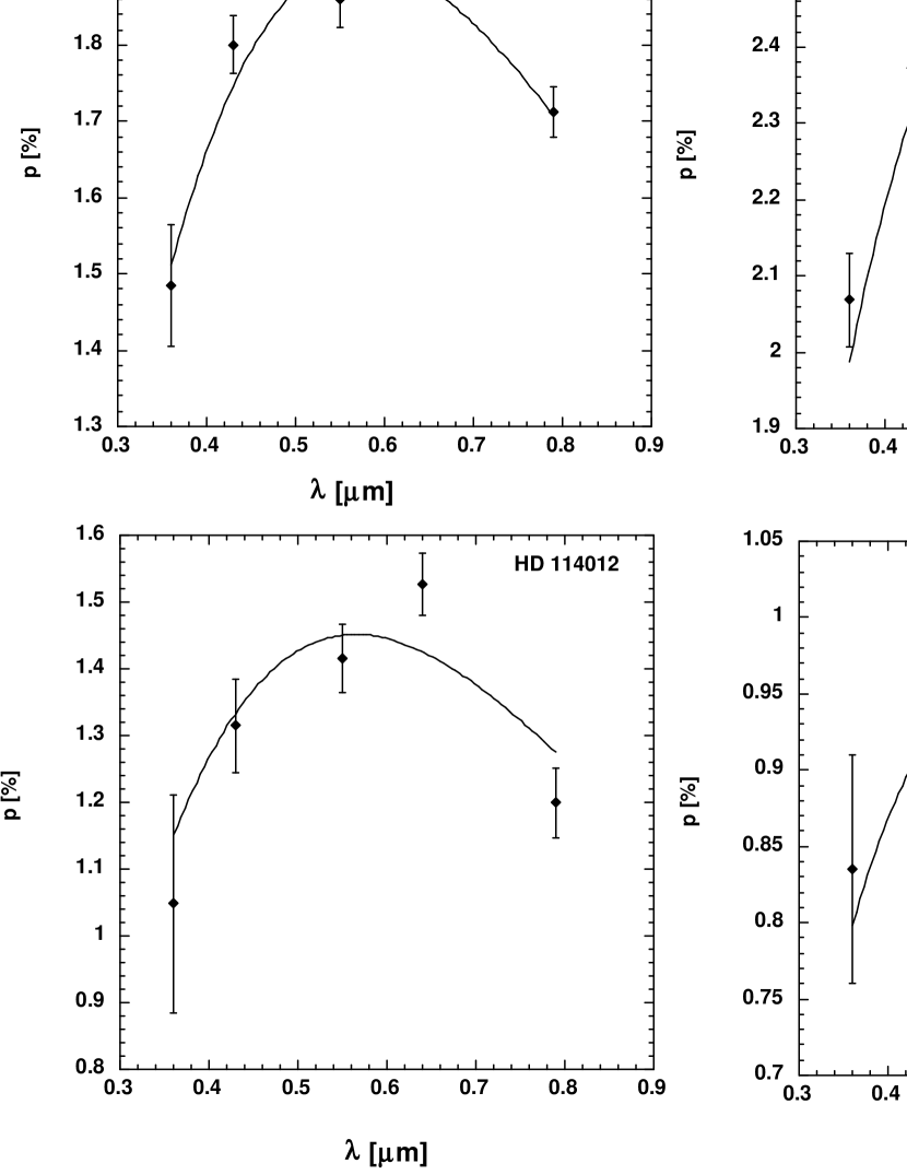
Table 3 list the best-fit parameters for the polarization curve fits for the Coalsack stars. Since we do not have any Near Infrared polarimetry for the Coalsack stars, special care is needed to potentially justify the use of Wilking fits. For these stars we show the reduced $\chi^{2}$ for the fits. We note that while the F-test justifies the additional free parameter of the Wilking fit for several stars, in most cases the reduced $\chi^{2}$ for these fits are then less than unity. The data and best-fit polarization curves are shown in Figure 1.

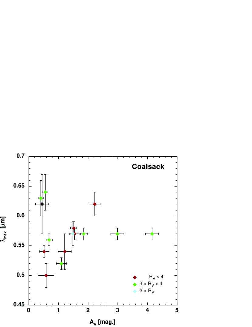
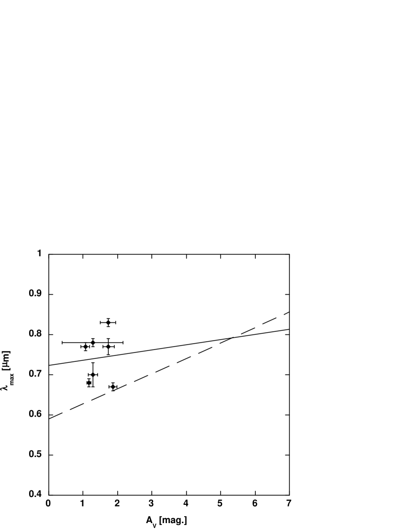
For HD 110432, the 2MASS data is flagged as being of poor quality, we therefore used an average of the results from Whittet & van Breda (1980), Dachs & Wamsteker (1982) and Dachs et al. (1988) for this star. In Figure 2 we plot the location of the derived wavelength of maximum polarization ($\lambda_{max}$) as a function of visual extinction. As noted above, earlier studies of the dependence of $\lambda_{max}$ on extinction parameters have found a relationship with the value of total-to-selective extinction (R_V; e.g. Whittet & van Breda (1978)). We do not find such a correlation for the Coalsack data. In Figure 2, we have color-coded the sightlines according to their R_V values. While the two sightlines above A_V=2.5 show R_V consistent of the value found at large visual extinction in this cloud (R${}_{V}\approx$3.25), no systematic trends in R_V are evident at smaller A_V.

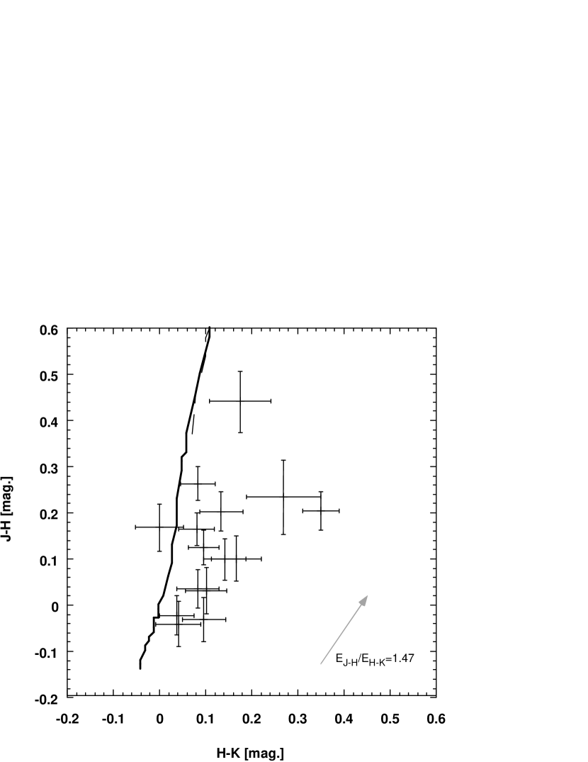
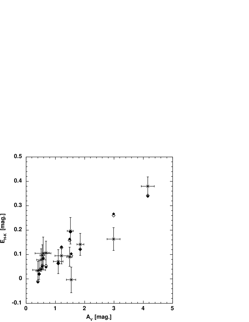
One possible caveat to the accuracy of the calculated R_V values comes from the fact that several of the target stars are in some spectral classifications listed as either emission line stars or possible binaries. To evaluate the possible influence of these complications for the Coalsack sample we used the J-H vs. H-K diagram, plotted in Figure 3. Since the direction of the reddening vector in this color-color diagram varies between regions (e.g. Racca et al. (2002)) we calculated the H-K color excess that, for each target gave the smallest offsets between measured colors and best-fit reddened colors, given the spectral classifications of the stars and direction of the reddening vector. We used E_J-H/E${}_{H-K}\approx$1.57 (Kenyon et al., 1998) and E_J-H/E${}_{H-K}\approx$1.91 (Naoi et al., 2006) as test cases. In Figure 4 we plot the H-K color excess versus the derived visual extinction. The measured difference (H-K)-(H-K)₀ is plotted a x:es with error bars. Open symbols represent the color excesses calculated assuming E_J-H/E${}_{H-K}\approx$1.57, while filled diamonds represent the color excesses calculated assuming E_J-H/E${}_{H-K}\approx$1.91. Only for HD 112661 and HD 112045 are offsets of more than 2$\sigma$ seen between the measured and best-fit H-K color excesses (2.1 and 2.2$\sigma$, respectively for E_J-H/E${}_{H-K}\approx$1.91). While both of these stars are listed in SIMBAD as multiple, neither shows an exceptional R_V value. Even if these sightlines are suppressed, no correlation between $\lambda_{max}$ and R_V is seen.

3.1.2 Chamaeleon, Musca, Ophiuchus, R CrA and Taurus Cloud Data

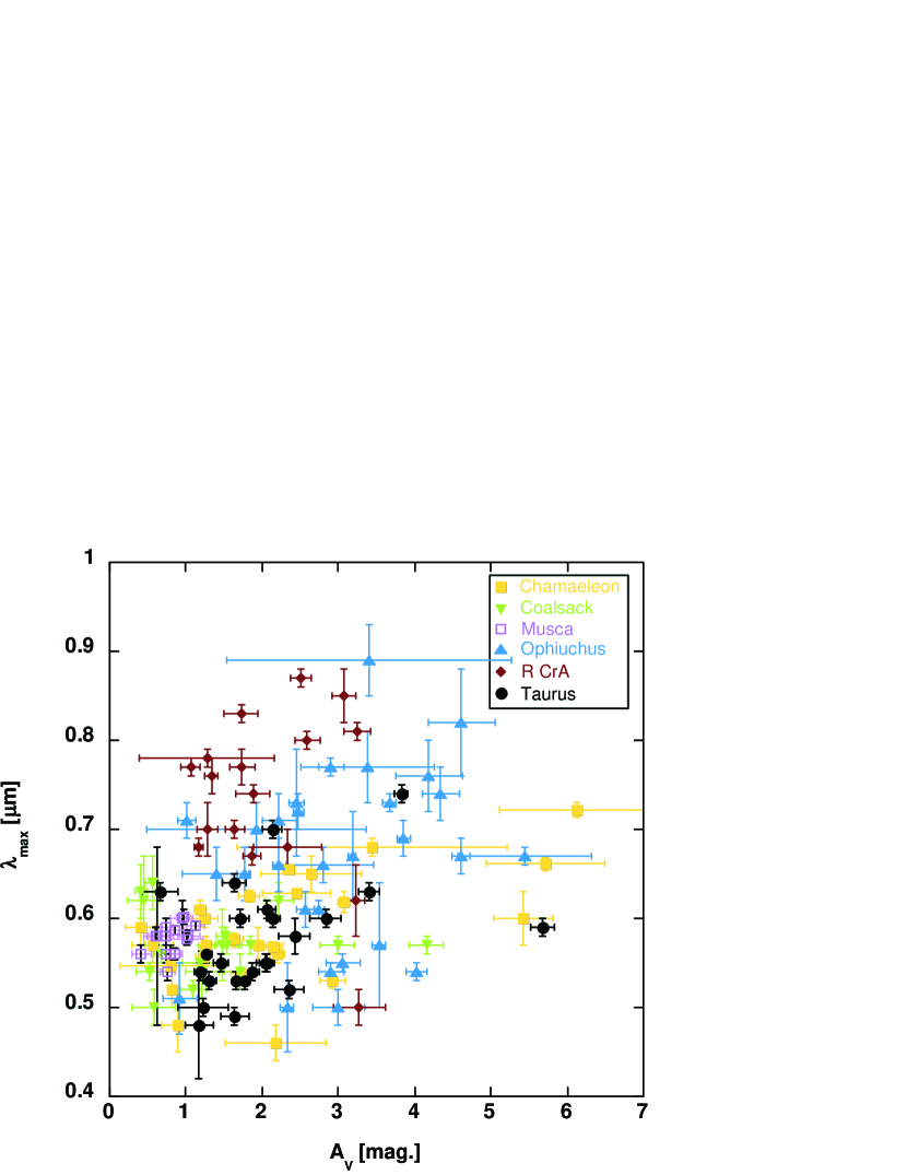
Figure 2 shows a tight correlation of $\lambda_{max}$ with A_V over the limited range of A${}_{V}\sim$1.0-2.5 but with outliers both at smaller and larger values of A_V. A similar weak correlation was noted by Whittet et al. (2001) in their Taurus data, but with a more pronounced scatter. To investigate whether the outlier points in the Coalsack plot are truly outliers in a real correlation, or whether the perceived correlation is instead a statistical fluke, we searched the literature for high quality, multi-wavelength polarimetry in sightlines penetrating well defined interstellar clouds.

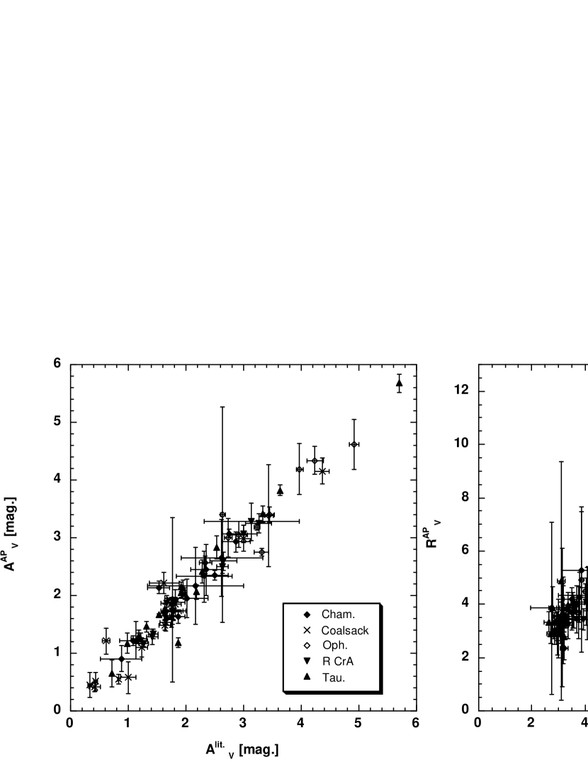
We selected five additional well-studied clouds with high quality published multi-wavelength polarimetry. Polarimetry data were extracted from the studies by: Chamaeleon; Whittet (1992) & Covino et al. (1997), Musca; Arnal et al. (1993), Ophiuchus; Whittet (1992) & Vrba et al. (1993), R CrA; Whittet (1992) and Taurus; Whittet (1992), Whittet et al. (2001). To ensure as uniform a dataset as possible in term of photometry and stellar characteristics, we extracted visual (B,V) and near-infrared data from the Tycho and 2MASS archives. We verified, and where possible updated the spectral classification, and then assigned intrinsic colors as for the Coalsack stars. The resultant stellar characteristics are listed in Table 4. In a couple of cases unphysical values of - in particular - R_V are encountered, likely indicating problems with the spectral classification. These sightlines were therefore excluded from the subsequent analysis. In Figure 5 we compare the values of R_V and A_V derived here with those extracted from the literature. For both parameters, good agreement is seen. We note that the R_V values quoted in Arnal et al. (1993) are based on polarimetry and not on photometry and we have therefore not included them in these plots.

As for the Coalsack sightlines, we fitted Serkowski or Wilking functions to the polarization data, but selected only those stars with polarization measurements in at least 4 filters (for this reason we also chose not to include the Chamaeleon data from Whittet et al. (1994)). The polarization fit parameters are given in Table 5. In most cases the $\lambda_{max}$ derived here agree with those in the original papers within 1$\sigma$ of the mutual uncertainties and in all but one cases within 2$\sigma$. The one exception is the sight line towards HD 107875 in Musca (star number 7 in the nomenclature of Arnal et al. (1993)), where the original paper reports $\lambda_{max}$=0.641$\pm$0.009 $\mu$m while we find $\lambda_{max}$=0.49$\pm$0.01 $\mu$m using their stated polarization curve parametrization. Given this discrepancy we have excluded this sightline form the analysis.

Plotting $\lambda_{max}$ vs. A_V for all six clouds (Figure 6), we see that, particularly for Chamaeleon, Musca and Taurus, a very similar structure is evident as for the Coalsack with a main grouping of point lying along what seems like a linear correlation from A${}_{V}\sim$1 to $\sim$2.5 mag. but with outliers both at small and large A_V. A critical issue, then, is whether the points we have here designated ”outliers” are indeed that in a statistical sense, or whether, the suggested correlation of $\lambda_{max}$ with A_V over approximately 1 to 3 magnitudes of extinction is illusory.

As noted above, two independent ways exist for estimating the extinction for a given parcel of gas and dust. However, neither the directly measured visual extinction, nor the color-temperature of the FIR emission from the heated grains are immune to biases. We will next discuss how the combination of the two tracers of extinction can be used to mitigate biasing in the determination of the effective opacity.

3.2 Effective extinction vs. line-of-sight extinction

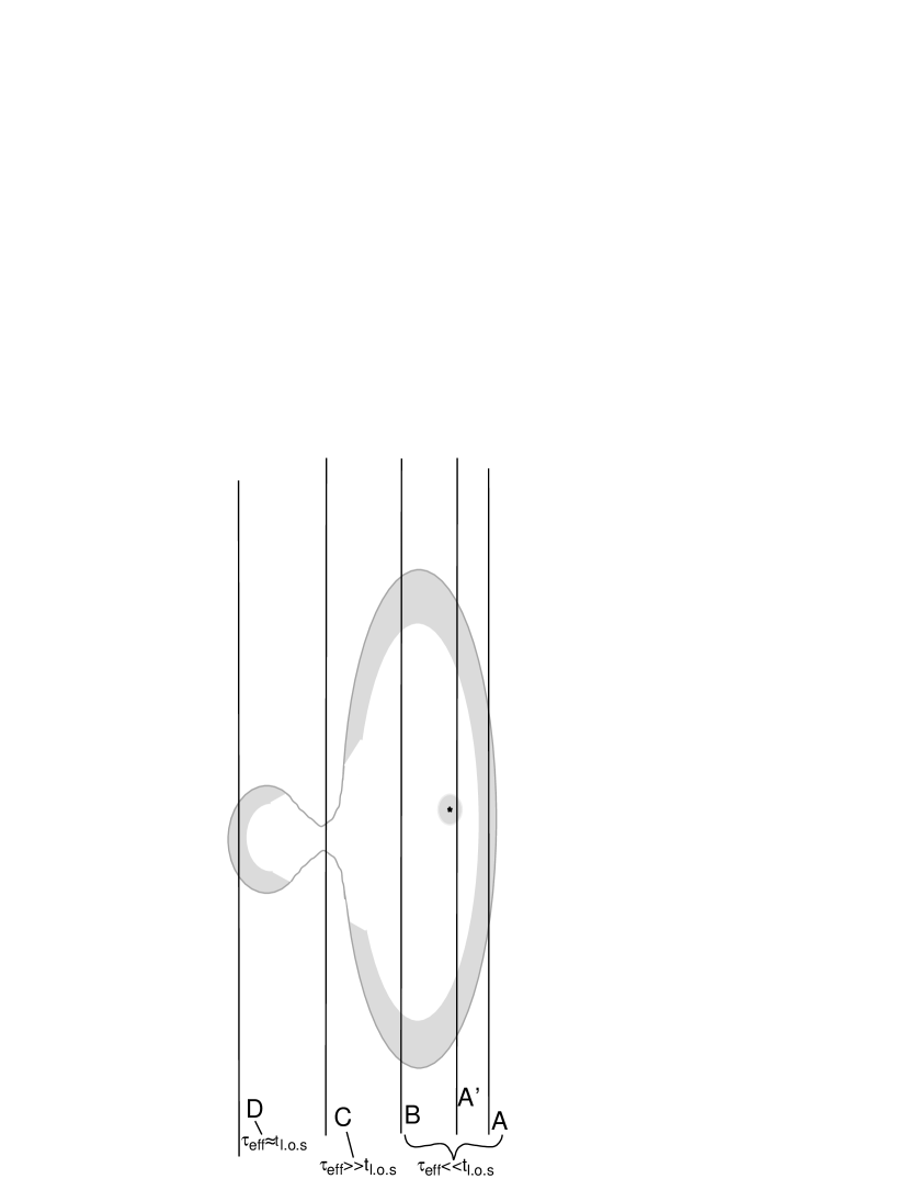
The line-of-sight extinction might not be a good indicator of the extinction - or equivalently, radiation field - seen by the material sampled by an absorption (line or continuum) experiment - the ”effective extinction”. Figure 7 illustrates some of the ways in which such discrepancies might occur. In this cartoon, we show a prolate cloud pointing towards the observer next to a roughly spherical cloud, with a ”bridge” of material linking the two. The gray zone is meant to illustrate the part of the cloud into which the interstellar radiation field penetrates.

For sightline ’A’, which passes through the outskirts of the prolate cloud, the line of sight extinction is much larger than the effective extinction seen by the material probed. The average radiation field seen by different parcels along the chord is similar and hence we’d expect this kind of sightline to show a large A_V while retaining a relatively large 60/100 ratio. A similar effect might arise if the sightline passes within the sphere of influence of an embedded, or nearby, stellar source contributing to the radiation field (A’).

For sightline ’B’ the line of sight extinction, again, is larger than that seen by the material, but here, the different parcels along the chord see very different radiation fields. For this kind of sightline we would again expect a large A_V but here - since the FIR radiation traces booth radiatively heated dust and dust in the dark part of the cloud - expect a low 60/100 ratio.

For sightline ’C’, which passes through a region between clouds (or in an inter-clump region of a clumpy medium) the line of sight extinction instead underestimates the effective extinction experienced by the material due to shadowing effects by the surrounding clouds.

Finally, in sightline ’D’ the observed and effective extinctions are similar and the different parcels of material along the chord experience similar radiation fields.

Similar effects and observational discrepancies might also arise in a clumpy medium with the sightlines passing through predominantly clump or inter-clump material.

3.3 Far Infrared Data

Empirically an anti-correlation is seen between column density and dust temperature based on the 60-to-100 $\mu$m ratio in interstellar clouds (see, for instance figure 8 of Snell et al. (1989)). Since this ratio therefore indirectly traces the radiation field seen by the dust, we can use it as a probe of the ”effective extinction” seen by the grain. While this emission is also likely prone to biases, such as variations in the fraction of small grains, we show in Appendix A that we can use the combination of visual extinction and Far Infrared (FIR) emission to screen the data sets for anomalous sightlines. We note that in this study we only do this in a relative sense for each cloud. We are not attempting to find absolute dust temperatures. While we will limit our analysis to the 60-to-100 $\mu$m ratio, we will use the 25-to-100 $\mu$m and 12-to-100 $\mu$m ratios to argue in Appendix A that the local changes seen in the relation between the 60-to-100 $\mu$m ratio and A_V are indeed likely due to irradiation differences.

We extracted FIR data from the IRIS re-reduction (Miville-Deschênes & Lagache, 2005) of the IRAS all-sky photometry. The spatial resolution of the IRIS maps are 3.8, 3.8, 4.0 & 4.2 arc-minutes respectively for the 12, 25, 60 and 100$\mu$m bands, but the maps are pixelized on a 1.5’ scale and hence over-sampled by about a factor of 2.5-2.8. For the current study we used a 3x3 pixel average that allows us to both lessen the impact of any emission from the background star and to identify it, if significant. Comparing to the IRAS point (faint) source catalog, we find that, in most cases, the stars - when at all detectable - make only a minor contribution to the total FIR light on our lines of sight. This is especially true of the longer wavelength bands.

Since the nominal, single pixel, photometric uncertainty in the IRIS maps is much smaller than the typical pixel-to-pixel variations (cf. Miville-Deschênes & Lagache (2005)), we found that the standard deviation in the 3x3 pixel averages can be used as a sensitive indicator of stellar contamination of the FIR flux densities, complementing the IRAS point source and faint source catalogs. For those sightlines where the background star - or a nearby star - contributes to the average, the standard deviation increases dramatically compared to the norm.

3.3.1 Nominal A_V vs. I(60$\mu$m)/I(100$\mu$m) relations

We can probe the difference between line of sight and effective extinction by comparing the observed visual extinction to the amount of emission due to heated grain, as probed by the ratio of 60$\mu$m to 100$\mu$m flux densities. To find a nominal relationship for each cloud, we used sightlines with reliably determined visual extinctions and compared these to the FIR data. We used two partially overlapping data sets for this analysis: Field stars were first selected from the Hipparcos catalog, providing trigonometric parallaxes and thus allowing a clean separation of the stars into groups foreground and background to the cloud, but with a fairly limited total number of sightlines. We also used the catalog of Tycho stars with known spectral classifications (Wright et al., 2003) to maximize the number of sightlines used. In this case, we usually do not have explicit distance information and we therefore imposed somewhat more stringent selection criteria for which stars to include in the analysis.

For the first field-star samples we selected all stars in the Hipparcos catalog within a three degree radius of l,b=(297,-15.5), (354, 15), (0,-19.5), (174,-14) and for the Chamaeleon, Ophiuchus, R CrA and Taurus clouds respectively. For the Musca cloud we used a two degree radius centered on l,b=(301, -8). For the Coalsack, we used the target list of Seidensticker (1989) as input in our Hipparcos search. From these original lists we then selected stars at distances (based on the Hipparcos trigonometric parallaxes) greater than those estimated for the clouds. Complementing the Tycho photometry with 2MASS NIR photometry we calculated visual extinctions. We rejected stars with negligible extinction and were left with samples of 39, 30, 23, 34 and 27 field stars for Chamaeleon, Musca, Taurus, R CrA and Ophiuchus clouds respectively.

For the second sample we selected stars as above from the catalog of Wright et al. (2003) for Chamaeleon, Coalsack, Musca, Ophiuchus and R CrA. For Taurus - because of the elongated shape of the cloud - we selected stars within a three degree radius of two centers at RA,Dec=(04:40:00,25:30:00) and (04:15:00,28 00 00). As with the Hipparcos sample, we extracted Tycho and 2MASS photometry, and calculated visual extinctions and ratios of total-to-selective extinctions. Based on A_V vs. distance diagrams from the Hipparcos samples, we then selected only those stars with A${}_{V}>${0.3, 0.4, 0.4, 0.4, 0.3 and 0.5} for Chamaeleon, Coalsack, Musca, Ophiuchus, R CrA and Taurus respectively. We used the IRAS point- and faint-source catalogs to screen out stars detected as point sources and finally screened for unreasonable values of R_V, which likely reflect unreliable spectral classifications. Finally, we eliminated small regions (usually 0.5 or 1 degree radii) around stars where the I₆₀/I₁₀₀ ratio showed localized influence from those stars (see Appendix A). We were then left with 90, 231, 60, 58, 96 and 154 stars respectively for the six clouds.

Because of the relatively bright limiting magnitude of the Hipparcos database, the size of the area used to select the field stars involves a trade-off between the largest acceptable distance from the cloud center and number statistics. While the polarization samples do cover smaller areas on the sky, the three-degree radius (two degrees for Musca) was chosen based on emission-line and extinction maps (e.g. Cambrésy (1999)). Although we do not have kinematic data tracing the material giving rise to the extinction in the field star samples, we can use the measured A_V values to see that this sample likely does probe the outer layers of the molecular clouds under study. Our Hipparcos field star samples have visual extinctions of A_V{min, max,mean}={0.3,2.4,1.0} mag. for Chamaeleon, {0.1,2.4,0.9} mag., for the Coalsack, {0.4,1.7,0.77} mag. for Musca, {0.4,4.5,1.6} mag. for Ophiuchus, {0.1,1.7,0.6} mag. for R CrA and {0.4,3.3,1.3} mag. for Taurus. As shown by Savage et al. (1977) and Rachford et al. (2002) the transition to molecular hydrogen occurs already at E${}_{B-V}\sim$0.1 (A${}_{V}\sim$0.3) and hence most of our field star sightlines probe molecular material. In addition, as shown by e.g. Wannier et al. (1983), van der Werf et al. (1989) and Andersson & Wannier (1993), molecular clouds are surrounded by extensive atomic envelopes. Figure 3 of Boulanger et al. (1998) also illustrates this for the Chamaeleon complex. Particularly for the high-latitude clouds in our study, it is thus unlikely that the field stars probe material unrelated to the clouds probes by the polarimetry.

As we are explicitly searching out, and expecting to find, points where the systematic errors dominate the random ones, we used a robust fitting algorithm (Press et al. (1986), p 539ff) to find the nominal I(60$\mu$m)/I(100$\mu$m) vs. A_V relations for each cloud. This algorithm uses an iterative procedure based on Tukey’s Biweight weighting with a limit of 6 outlier-resistant standard deviations (Press et al., 1986), as implemented in the IDL routine ”robust_linefit”, available in the ”astron” library. For the larger Tycho sample we also used weighted linear fits. The two algorithms yield very similar fitting parameters in this case.

For the Hipparcos samples, the robust fits for Chamaeleon, Musca, Ophiuchus, R CrA and Taurus yield:

$$I_{60}/I_{100}=\begin{array}[]{c}(0.241\pm 0.005)\\ (0.29\pm 0.01)\\ (0.27\pm 0.02)\\ (0.21\pm 0.01)\\ (0.196\pm 0.008)\end{array}-A_{V}\times\begin{array}[]{l}(0.022\pm 0.005)\ [Cham]\\ (0.026\pm 0.010)\ [Musc]\\ (0.01\pm 0.02)\ [Oph]\\ (0.035\pm 0.01)\ [R~{}CrA]\\ (0.013\pm 0.006)\ [Tau]\end{array}$$ (3)

For the Tycho samples, the robust fits yield:

$$I_{60}/I_{100}=\begin{array}[]{c}(0.240\pm 0.004)\\ (0.29\pm 0.1)\\ (0.27\pm 0.1)\\ (0.244\pm 0.006)\\ (0.179\pm 0.003)\end{array}-A_{V}\times\begin{array}[]{l}(0.018\pm 0.004)\ [Cham]\\ (0.030\pm 0.007)\ [Musc]\\ (0.024\pm 0.010)\ [Oph]\\ (0.023\pm 0.007)\ [R~{}CrA]\\ (0.012\pm 0.002)\ [Tau]\end{array}$$ (4)

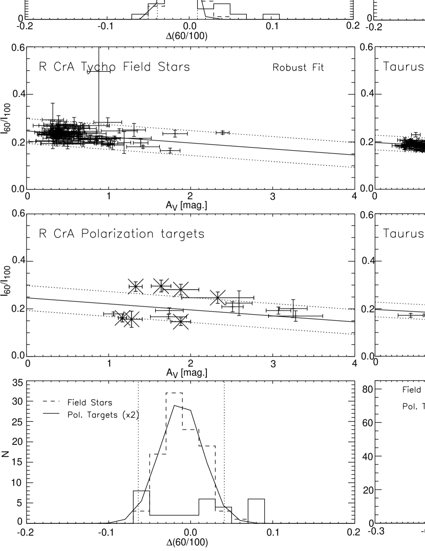
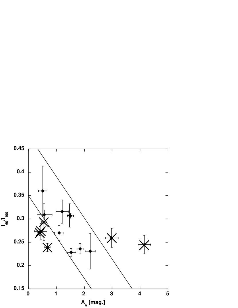
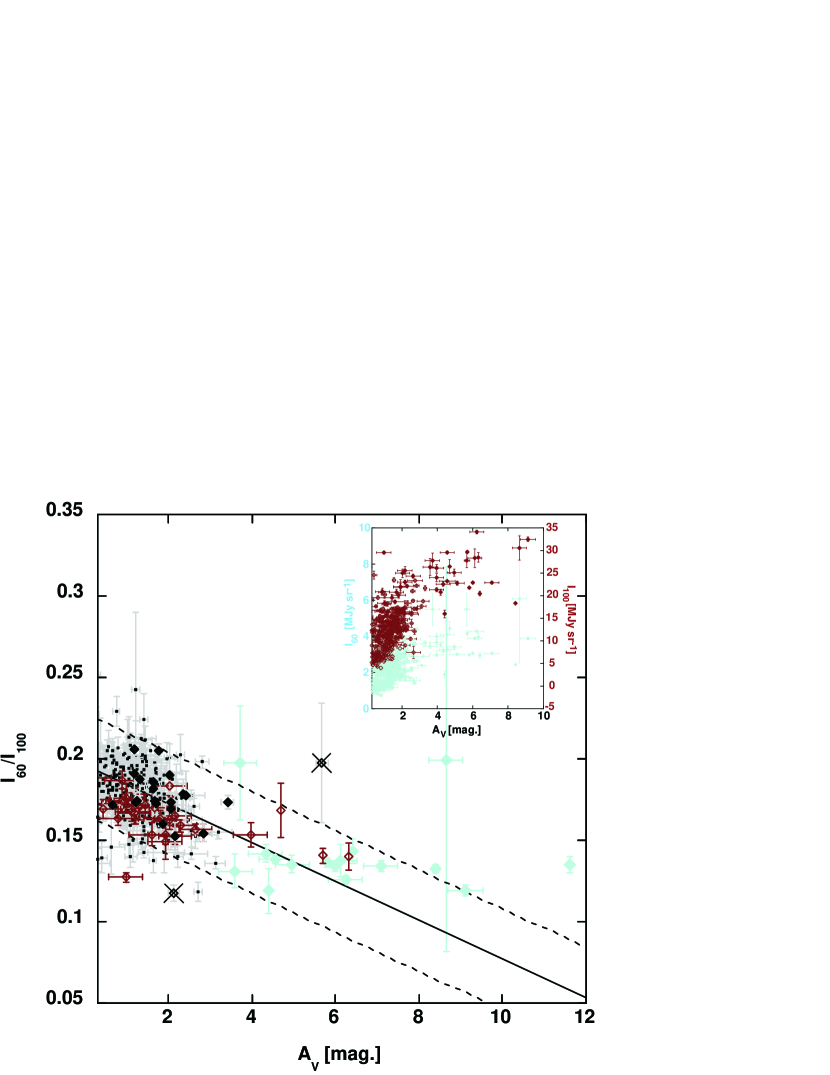
In Figure 8 we show the best linear fits (solid lines, top panel) using the robust fitting algorithm to the Tycho field star samples only (i.e. the polarization targets were not included in the fits).

For Chamaeleon, Musca, Ophiuchus, R CrA and Taurus well-defined linear correlations are found (for Ophiuchus, the uncertainties on the fit coefficients for the Hipparcos sample, are too large for the fit to be significant). For the Coalsack, which straddles the Galactic plane, this technique fails to provide a reasonable correlation, presumably because of the strong influence of diffuse background sources in the FIR data.

The middle panels of Figure 8 shows the locations of the polarization targets in the FIR vs. A_V diagrams.

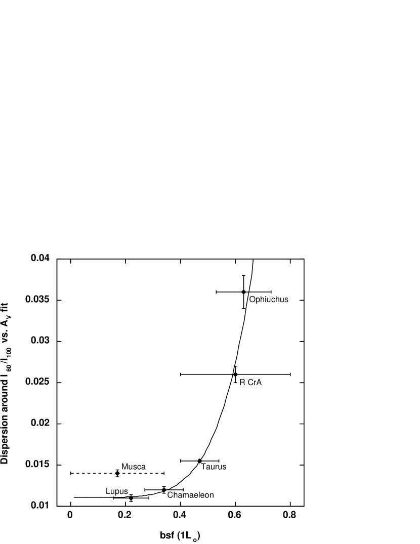
In the lower panels of Figure 8, we show the distributions of offsets in I₆₀/I₁₀₀ from each data point to the best fit line at the same value of A_V (dashed histograms for the field stars and solid histograms for the polarization targets), and the best fit Gaussians to these distributions. The widths of the distributions are similar for all clouds ($\sigma$=0.012, 0.014, 0.036, 0.026 and 0.016, respectively). Based on similar geometrical arguments as for Figure 7, it is likely that these widths trace the porosity of the outer parts of the clouds where the radiative grain heating occurs. In Appendix A we show that the widths of these dispersions are correlated with the SFR in the clouds.

The dashed lines in Figure 8 show the 2$\sigma$ distance from the best-fit solution. Points below and to the left of the left-hand dashed lines are likely to have characteristics of sightlines ’B’ in Figure 7, for high values of A_V, or ’C’, for low values of A_V, while points above and to the right of the right-hand dashed lines are likely to have characteristics of sightlines ’A’.

We note that with the exception of the identified outliers, the polarization sample targets and the field stars overlap in the well-defined Gaussian distributions in offset from the fits, providing additional support for the assumption that the two observational samples are drawn from a common parent population.

While the above screening method fails for the Coalsack, inspecting the $\lambda_{max}$ vs. A_V plot for the Coalsack and comparing it to those of Chamaeleon and Taurus, we can see that the points at relatively high extinction and relatively low $\lambda_{max}$ in the Coalsack have corresponding sightlines in both Chamaeleon and Taurus and that these sightlines in the Coalsack fall in the equivalent ”A” region in the I₆₀/I₁₀₀ vs. A_V plot as their counterparts for Chamaeleon and Taurus. Similarly, the points at high $\lambda_{max}$ and low A_V are similar to points in region ”C” for Chamaeleon both in the $\lambda_{max}$ vs. A_V and I₆₀/I₁₀₀ vs. A_V plots. While based on a more indirect and less satisfactory procedure, we therefore screen these points also in the Coalsack sample. In Figure 9 we show the resulting I₆₀/I₁₀₀ vs. A_V plot with the sources thus deselected marked. The width of the $\Delta$I₆₀/I₁₀₀ distribution for the remaining sightlines for the Coalsack is $\sigma$=0.04 also similar to the values found for the other clouds.

4 Results and Discussion

4.1 Origin of the Outliers

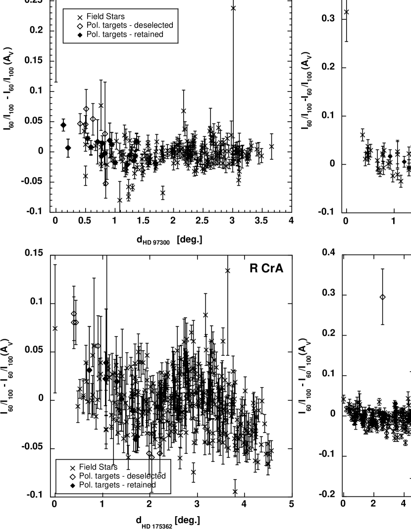
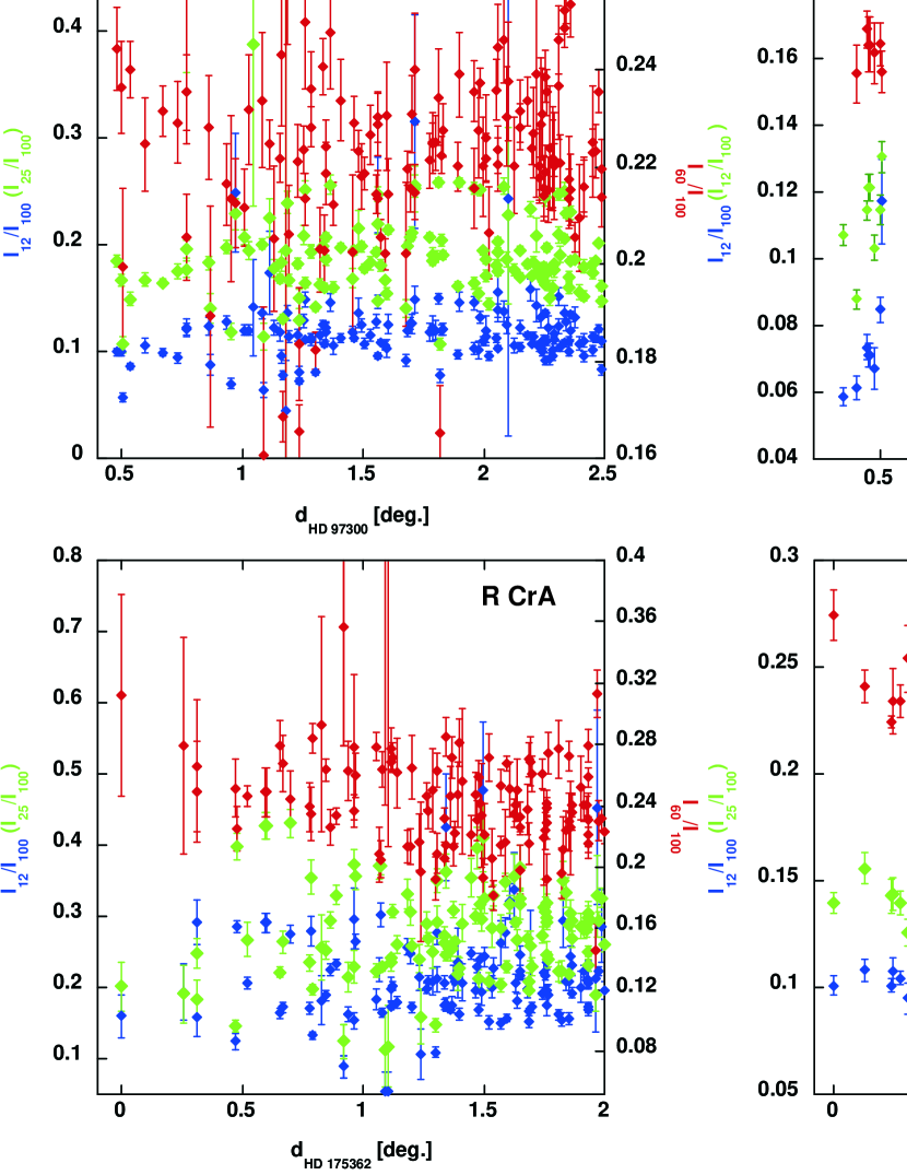
We argue that the outliers in figure 8 are likely primarily due to localized differences in the irradiation of the dust. Appendix A provides several direct lines of evidence in favor of this interpretation. For Chamaeleon and R CrA all the sightlines identified as type ”A” can be seen to be due to proximity to HD 97300 or HD175362, respectively. Similarly, for Ophiuchus almost all type ”A” sightlines can be seen to be close to either $\sigma$ Sco or $\rho$ Oph D (Figure 10). Additionally, as also shown in appendix A, the ratio I₆₀/I₁₀₀ shows a stronger response to the vicinity of a hot star than I₂₅/I₁₀₀ while the I₁₂/I₁₀₀ ratio shown little or no response to the proximity of hot stars. These results provide strong support for an origin in irradiation differences. As shown in Appendix A the dispersion around the best-fit lines in the I₆₀/I₁₀₀ vs. A_V plots are correlated with the characteristics of the star formation in the cloud (see below). We interpret this as due to increasing porosity (clumpiness) in the clouds produced by increasing star formation activity, which changes the radiative transfer of the light heating the dust grains. A quantitative analysis of this clumpy transfer is beyond the scope of the present paper.

It should be noted that the screening procedure used in figure 8 does not rely on this interpretation. The screening as such is a straightforward numerical procedure and uses a explicit numerical limit for which sightlines to label ”anomalous”. The use of the I(60$\mu$m)/I(100$\mu$) vs. A_V ratio to screen the polarimetry data should also not introduce any biases in the latter. This is as only a very small fraction of the grains contribute to the polarization (Kim & Martin, 1995) while all grains contribute to the FIR emission. Also, even if the outliers in figure 8 were due to significant enhancements in the population of very small grains, the size distributions of the VSGs and the grains responsible for the visual polarization have, at most, a minute overlap (Kim & Martin, 1995; Desert et al., 1990).

4.2 Debiased $\lambda_{max}$ vs. A_V plots

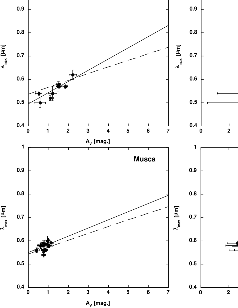
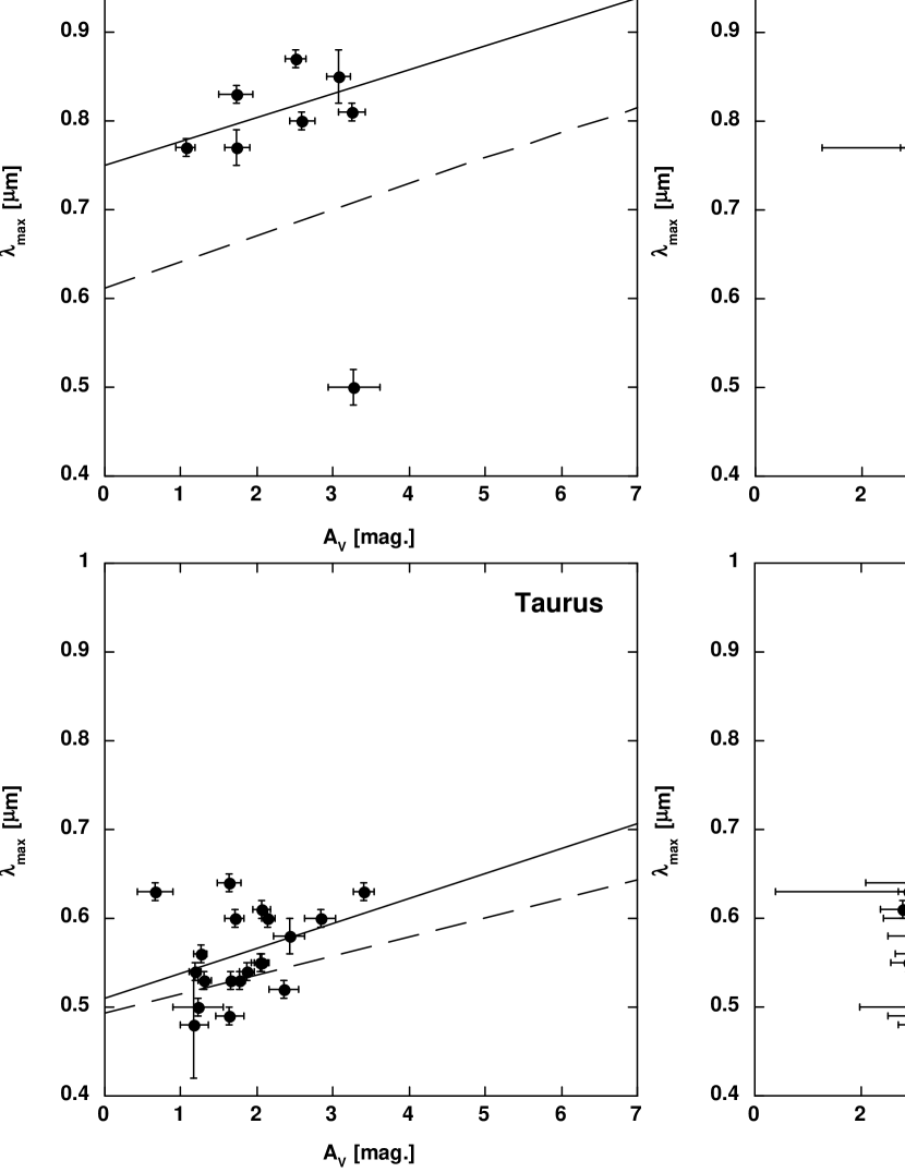
In Figure 11 we show the plots of $\lambda_{max}$ vs. A_V which result if we reject the points in Figure 8 which falls more than 2$\sigma$ from the robust fits for the Tycho sample. Overlaid are the best linear fits for each cloud (full drawn lines). The dashed lines represent the relations based on the average slope from all the clouds and a zero intercept based on the mean value of R_V of the cloud (see below). Very similar plots result for the Hipparcos based screening, with the main difference that the R CrA sample shows a broader scatter. We show the $\lambda_{max}$ vs. A_V plot for R CrA using the Hipparcos screening in Figure 13. In what follows, we will, except were explicitly noted, discuss these ”de-biased” data sets.

Three conclusions can immediately be drawn from these new plots:

1) While the plot of $\lambda_{max}$ vs. A_V including all the data shows only a very weak correlation, the ”screened” plot shows a distinct correlation of $\lambda_{max}$ with A_V for Chamaeleon, Coalsack, Musca and Taurus and consistent results for Ophiuchus and R CrA. We can quantify this latter statement by performing Spearman rank order tests on the two groups of data sets. For Chamaeleon and Taurus both the unscreened and Hipparcos screened data sets show small ($<$6%) probabilities for being uncorrelated (the Tycho screened sets yield 2% and 14% probabilities). For the Coalsack the probability for an accidental correlation drops from 44% to 6% after screening. For Musca (where no sightlines are screened) we find a 18% probability of being uncorrelated.

2) Within each individual cloud sample, no obvious correlations are seen between $\lambda_{max}$ and R_V.

3) It now is clear to the eye that the slopes of $\lambda_{max}$ vs. A_V in the individual clouds are very similar, but the three groups are offset from each other in $\lambda_{max}$. We used robust fits to quantify this and find that for the Hipparcos screened sample:

$$\lambda_{max}=\begin{array}[]{c}(0.54\pm 0.02)\\ (0.50\pm 0.02)\\ (0.55\pm 0.02)\\ (0.60\pm 0.05)\\ (0.72\pm 0.10)\\ (0.48\pm 0.02)\end{array}+A_{V}\times\begin{array}[]{l}(0.04\pm 0.01)\ [Cham]\\ (0.05\pm 0.01)\ [CS]\\ (0.04\pm 0.02)\ [Musc]\\ (0.01\pm 0.03)\ [Oph]\\ (0.01\pm 0.08)\ [R~{}CrA]\\ (0.05\pm 0.01)\ [Tau]\end{array}$$ (5)

While for the Tycho screened sample:

$$\lambda_{max}=\begin{array}[]{c}(0.54\pm 0.01)\\ (0.50\pm 0.02)\\ (0.55\pm 0.02)\\ (0.64\pm 0.05)\\ (0.75\pm 0.03)\\ (0.51\pm 0.02)\end{array}+A_{V}\times\begin{array}[]{l}(0.024\pm 0.006)\ [Cham]\\ (0.05\pm 0.01)\ [CS]\\ (0.04\pm 0.02)\ [Musc]\\ (0.01\pm 0.03)\ [Oph]\\ (0.03\pm 0.02)\ [R~{}CrA]\\ (0.03\pm 0.02)\ [Tau]\end{array}$$ (6)

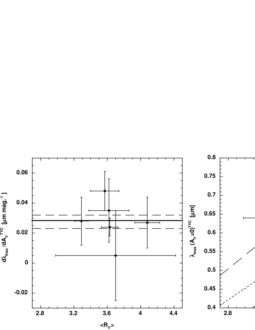
The slopes in $\lambda_{max}$ vs. A_V are all very close and, in particular, those for Chamaeleon, Coalsack, Musca and Taurus are all both very close and have small error bars, indicating that the slope is universal (Figure 14, left panel). A weighted average of the slopes yields d$\lambda_{max}$/dA_V=0.028$\pm$0.005 (0.038$\pm$0.007) for the Tycho (Hipparcos) screened samples.

As has been shown by Whittet & van Breda (1978) $\lambda_{max}$ is generally found to be correlated with R_V. This is not surprising as, as has been shown by Kim & Martin (1995) and Kim & Martin (1994), changes in both $\lambda_{max}$ and R_V are most sensitive to changes in the population (total and aligned part) of the smaller grains. In the right-hand panels of Figure 11 we plot $\lambda_{max}$ vs. R_V for the screened samples. No correlations are seen even for the clouds where correlation in the $\lambda_{max}$ vs. A_V plots are evident.

We calculated weighted averages of R_V for the full polarization targets samples and find R_V=3.6$\pm$0.1, 3.6$\pm$0.2, 3.6$\pm$0.2, 3.7$\pm$0.7, 4.1$\pm$0.2 and 3.3$\pm$0.1 for Chamaeleon, the Coalsack, Musca, R CrA and Taurus, respectively. In Figure 14 (right panel) we plot the result with the best linear fit of the zero-intercept of $\lambda_{max}$ ($\lambda_{max}$(A_V=0)) for the Tycho screened samples with the average R_V. The best, weighted, fit yields:

$$\lambda_{max}(A_{V}=0)=(-0.47\pm 0.16)+(0.28\pm 0.04)<R_{V}>$$ (7)

or, if we impose a zero intercept:

$$\lambda_{max}(A_{V}=0)=(0.151\pm 0.002)<R_{V}>$$ (8)

for the Hipparcos screened sample the equivalent fits yield:

$$\lambda_{max}(A_{V}=0)=(-0.26\pm 0.24)+(0.22\pm 0.07)<R_{V}>$$ (9)

or, if we impose a zero intercept:

$$\lambda_{max}(A_{V}=0)=(0.146\pm 0.002)<R_{V}>$$ (10)

In both cases the zero intercept fit is close to the $\lambda_{max}$=(0.18$\pm$0.01)R_V found by Whittet & van Breda (1978).

We interpret the correlation of $\lambda_{max}(A_{V}=0)$ with $<R_{V}>$ as being due to the underlying differences in the total grain size distribution between the clouds, and the (universal) slope in $\lambda_{max}$ vs. A_V as due to varying degrees of grain alignment at different depths into the clouds caused by a common mechanism.

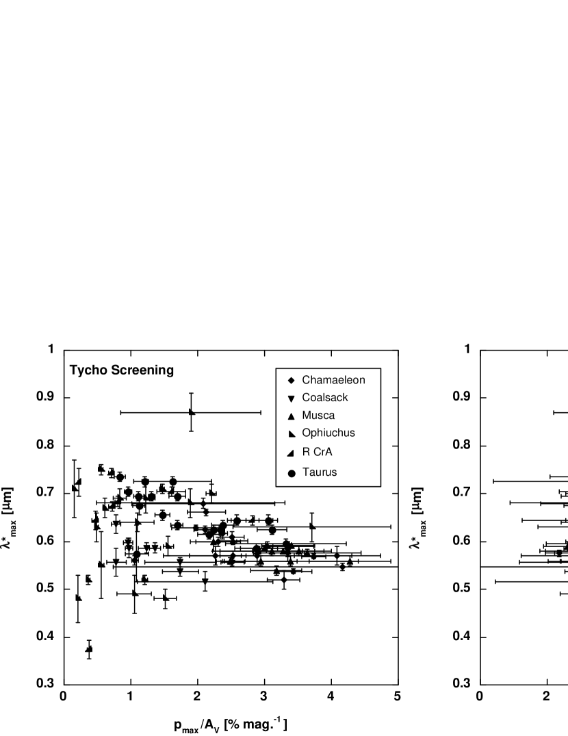
The data indicate that the lack of aligned small grains at larger visual extinctions, indicated by large values of $\lambda_{max}$, is due to loss of alignment rather than grain destructions. This can be seen by comparing $\lambda_{max}$ as a function of p_max/A_V and of R_V. In Figure 15 we show $\lambda_{max}$ for the Tycho screened lines of sight, adjusted to Chamaeleon, as functions of either the alignment efficiency (p_max/A_V) or R_V. The adjustment performed here consists of subtracting the difference in derived $\lambda_{max}(A_{V}=0)$ between the cloud and that for Chamaeleon for the sightlines in each cloud (i.e.: $\lambda_{max}^{*}$=$\lambda_{max}$-($\lambda_{max}$(A_V=0)^cloud-$\lambda_{max}$(A_V=0)^Cham.)).

A distinct anti-correlation (albeit, again, with outliers) is seen in the $\lambda_{max}$ vs. p_max/A_V (Figure 15, left panel), indicating that as the relative number of aligned grains increase the average size of the aligned grains decrease. No correlation is seen in the $\lambda_{max}$ vs. R_V plot (Figure 15, right panel) Very similar plots, again, result if we instead use the Hipparcos screened sample.

As equation 1 shows, when all other parameters remain fixed, the smallest grains will have their rotation damped out by gas collisions the fastest. Hence, when we find that smaller and smaller grains remain aligned either the damping is lessened or the driving mechanism for the spin-up in being enhanced. The correlations of $\lambda_{max}$ with A_V shows that as we get increasingly close to the cloud surface, smaller grains remain aligned. As has been shown on large scales for low radiation intensity cloud envelopes by Andersson & Wannier (1993); Wannier et al. (1999) and recently on small scales in the higher radiation field case of the Horse Head nebula by Habart et al. (2005), cloud envelopes show isobaric structures in the gas pressure and hence equation 1 becomes

$$t_{damping}\propto\frac{a\sqrt{T}}{P_{gas}}$$ (11)

with P_gas a constant for a given cloud.

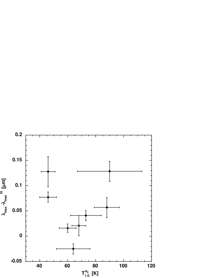
Hence an increase in temperature (assuming an isobaric equation of state) should lead to a decrease in $\lambda_{max}$. We searched the literature for Copernicus and FUSE measurements of the J=1/J=0 excitation temperature for the six clouds in our study. Unfortunately, only for Ophiuchus and Chamaeleon are there presently multiple interstellar sightlines published and not all of those sightlines have been studied in polarimetry. For Ophiuchus, five sightlines were studied by Snow & Jenkins (1980) with an additional two by Cartledge et al. (2004). These yield a range in 1-0 temperatures of 46 to 90 K. For Chamaeleon, Gry et al. (2002) report 1-0 excitation temperatures for three stars between 60 and 66 K. Rachford et al. (2001) report T=63 K for the line of sight towards HD110432 behind the Coalsack. For the five Ophiuchus sightlines with H₂ data, measured $\lambda_{max}$ can be extracted from Serkowski et al. (1975) while one of the Chamaeleon stars (HD 96675 $\equiv$ F24) and HD 110432 are included in the present data samples. In Figure 16 we plot both the measured values of $\lambda_{max}$ and the offset from the best-fit relations in $\lambda_{max}$ vs. A_V for each cloud. No clear correlation is apparent. We therefore conclude that variations in gas temperature are unlikely to explain the variations in the grain alignment.

Based on these observational results we conclude that the data support grain alignment driven by the radiation field. This conclusion is consistent with recent developments in the theory of interstellar grain alignment. Several authors (Draine & Weingartner, 1996; Weingartner & Draine, 2003; Cho & Lazarian, 2005) have shown that direct radiative torques are the theoretically most likely mechanism for explaining the spin-up of interstellar grains required to allow the magnetic alignment to take place.

We note, however, that our results cannot exclude alignment driven by molecular hydrogen formation (in steady state any formation of H₂ must be preceded by the radiative destruction of the molecule, and hence this mechanism is also more strongly active at smaller A_Vs). Indeed, if we use the models of Kim & Martin (1995) to estimate the smallest aligned grains at the surface of the clouds, using $\lambda_{max}$(A_V=0)$\approx 0.5~{}\mu$m, we find that grains as small as 0.01-0.04 $\mu$m need to be at least partially aligned. For silicate grains in a diffuse cloud environment, Table 5 of Draine & Weingartner (1996) shows that for such small grains, H₂ formation driving is dominant over direct radiative torques. We note though that according to Lazarian & Draine (1999) very small grains should flip frequently due to Barnett and nuclear relaxation. Thus under H₂ formation torques (fixed in the grain coordinate system) they are expected to become thermally trapped and not be able to achieve suprathermal spins. Further observational and theoretical studies are clearly needed to clarify the origin of the very small $\lambda_{max}$(A_V=0) we observe.

4.3 Influence of star formation

Figure 11 indicates that the scatter in $\lambda_{max}$ is related to the star formation activity of the cloud. We will here explore possible mechanism for this dependence, but start by noting that turbulence, and its associated line of sight variations in the magnetic field direction, is not a likely cause. This is because $\lambda_{max}$ is not, to first order, dependent on the absolute amount of polarization and since turbulence should affect the polarization in all bands similarly, leaving $\lambda_{max}$ unaffected.

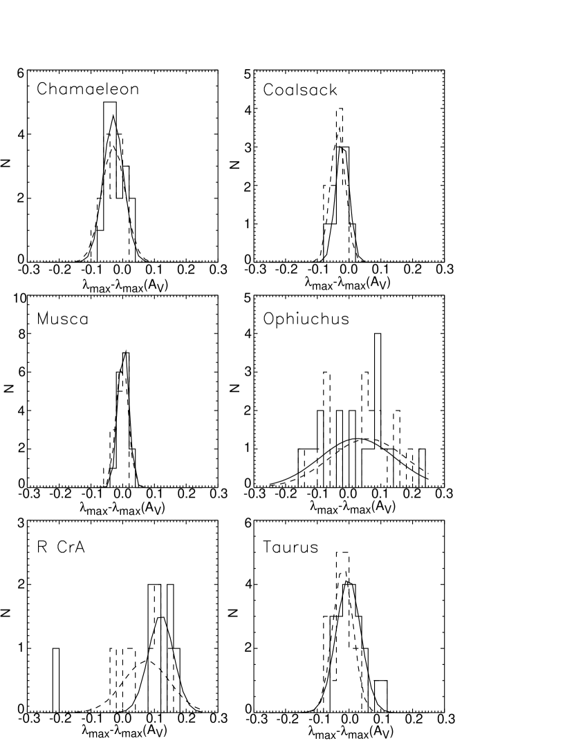
In Figure 17 we show histograms of the distance from the best fits in $\lambda_{max}$ with A_V for the six clouds using the ”universal slope” relations. As is clear by a visual inspection, the scatter increases from the Coalsack, Chamaeleon and Musca through Taurus to Ophiuchus and R CrA.

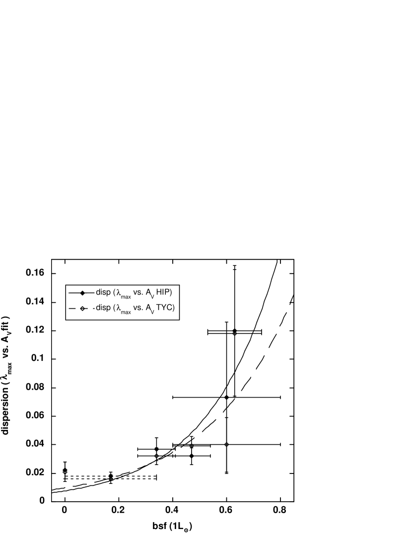
In Figure 18 we plot the scatter around the best fit in $\lambda_{max}$ with A_V as a function of the ”bright star fraction” (bsf(L${}_{bol}^{i}$)) of embedded Young Stellar Objects (YSO). The bright star fraction is defined as the number fraction of objects brighter than a given bolometric luminosity (L${}_{bol}^{i}$) to the total number of objects (cf Chen et al. (1997)). The error-bars on the bsf:s reflect counting statistics. The data for Chamaeleon, Ophiuchus, R CrA and Taurus are taken from Chen et al. (1997). For the Coalsack, which does not show any star formation, we here use bsf$\equiv$0. Musca has not been specifically studied for star formation activity although some T Tauri stars are detected in the general Chamaeleon-Musca complex (Mizuno et al., 1998). To separate the Coalsack and Musca points we have for plotting purposes assigned a bsf of 0.17 mid-way between Chamaeleon and the Coalsack. Neither point was used the fitting.

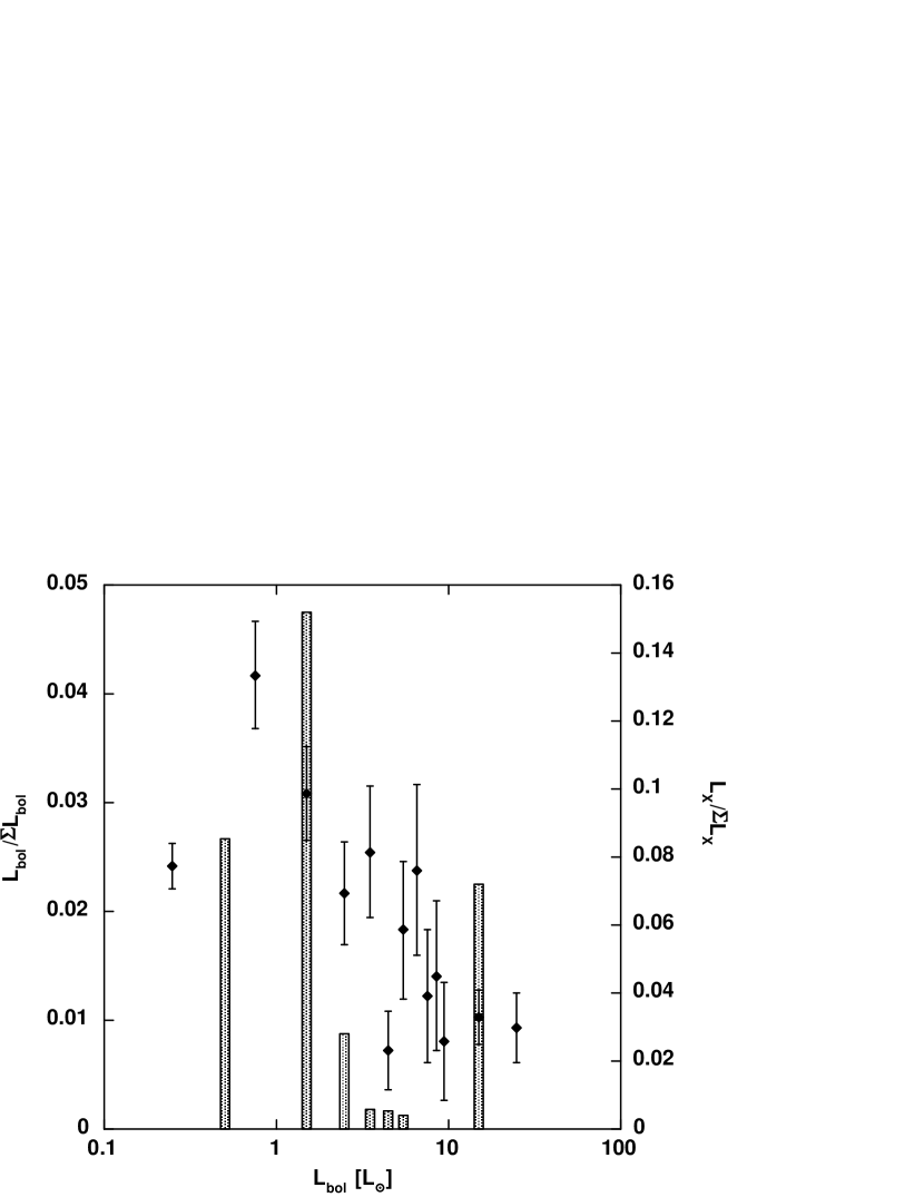
We used power law and exponential fits for several choices of the break-point (L${}_{bol}^{i}$; see above) in the bsf and find a best fit using an exponential for L_bol=1L_⊙, yielding a correlation coefficient of R=0.88 (for the Hipparcos screened sample and 0.79 for the Tycho screened sample) the resulting fit is over-plotted in Figure 18. At both smaller and larger L${}_{bol}^{i}$ the fit is worse. While not conclusive, this is consistent with an origin of the correlation due to the influence of the YSOs since the contribution, per unit luminosity range, to the total luminosity of the YSOs peaks around 1-2 L_⊙. This is illustrated in Figure 19 where we show the relative contribution to the bolometric and X-ray luminosity per unit L_bol for different sub-samples. The data for the bolometric luminosity are a combination of the data for Chamaeleon, Ophiuchus and Taurus, taken from Chen et al. (1995). The individual cloud data give similar results but with bigger scatter. The data for the X-ray luminosity are from Grosso et al. (2000). We chose a variable binning aimed at providing good resolution while collecting enough targets per bin to achieve reasonable statistic per bin. The relative binned bolometric luminosity peaks at $\sim$1 L_⊙ depending marginally on the exact binning, while the X-ray luminosity peaks at $\sim$1-2 L_⊙ with significant contributions from individual high luminosity stars. (The 10-20 L_⊙ bin however only contains two stars. We have also excluded target A21 from Grosso et al. (2000) with L_bol=1100_⊙ and log(L_X)=30.8 in the plot.)

In Taurus (and R CrA if using the Hipparcos screening) the outliers in Figure 17 are primarily located on the positive side of the plots. Depending on whether we use the Tycho or Hipparcos based screenings, the data for R CrA either shows a fairly wide dispersion or a significant offset in the center of the distribution. For Chamaeleon, the Coalsack, Musca and Ophiuchus, the average of the distances of points from fits are much less than their associated standard deviation. Also for Taurus the average offset is smaller that the standard deviation, but here the distribution has a statistically significant positive skew (Press et al. (1986), p. 457) of 0.66$\pm$0.53 (for the Hipparcos screening; 0.57$\pm$0.53 for the Tycho screening).

The scatter is likely due to porosity in the clouds, introduced by the effects of star formation, as seen in the dispersions between I₆₀/I₁₀₀ vs. A_V plots (Appendix A). However, for variations in the radiation field intensity caused by clouds porosity alone we would expect that the scatter be symmetrical. Particularly for Taurus and R CrA we are thus led to consider possible mechanisms which will drive $\lambda_{max}$ selectively to larger values, and hence also possible sources of additional, localized, grain rotation damping.

Given the ubiquity of X-ray emission from YSOs, it is worth considering what effects X-rays from the embedded YSOs would have on the grain rotation. One important X-ray induced effect is the ejection of photoelectrons from the grains and both the subsequent heating of the gas and charging of the grains. As shown by Draine & Lazarian (1998) the dominant rotation-damping mechanism in molecular cloud environments for very small grain (smaller than those discussed herein) is plasma drag due to the interaction between the ions in the gas and the electric dipole moment of the grain. Since the dipole moment of the grain is proportional to the grain charge (Draine & Lazarian, 1998), enhanced localized grain charging would also mean enhanced localized rotation damping, in addition to the enhancement from gas heating. If we extrapolate the molecular cloud (MC) panel of Figure 4 of Draine & Lazarian (1998) to the 0.05 $\mu$m range, we find that in the nominal model, neutral-gas drag is the dominant damping mechanism. However, plasma drag is only less important by a factor of a few. Hence, an increase in the grain charge by an order of magnitude would invert this relative importance. The typical X-ray (h$\nu$$\sim$0.5-5 keV) luminosity of embedded YSOs is 10³⁰-10³¹ ergs s^-1 with flares reaching significantly higher (Ozawa et al., 2005; Grosso et al., 2000).

To derive a first order estimate of whether X-rays from YSOs can significantly effect the grain rotation, we use the Ophiuchus cloud observations. In the observations of Grosso et al. (2000) for the inner part of cloud, 66 targets were found within an approximate radius of 15’, or at a distance of 140 pc, 0.6 pc, yielding a characteristic projected source-to-source distance of 0.075 pc. At this radius the X-rays from a single source contributes an energy density of about u=5$\times 10^{-16}$ ergs cm^-3. Draine & Lazarian (1998) assumed a energy density in the radiation field of the 1% of the nominal ISRF for their molecular cloud medium, or u$\sim$9$\times 10^{-15}$ ergs cm^-3 (Weingartner & Draine, 2001). Taking into account also the contributions of FUV emission from the YSOs, the high photoelectric yield at soft X-rays (Dwek & Smith, 1996) and the contributions from the diffuse X-ray emission, likely caused by stellar winds (Ezoe et al., 2006), we feel that the influence of embedded X-ray sources is a viable cause of the localized rotation damping and warrants further study. However, observational studies and modeling, beyond the scope of the present paper, are required to quantify the importance of X-ray induced grain rotation damping.

5 Conclusions

We have used new multi-band polarimetry of the Southern Coalsack to study the alignment of interstellar grains. For this study the Coalsack has the advantage of not showing a systematic increase in the total-to-selective extinction, R_V with increasing visual extinction and to show no star formation. The former allows us to break the degeneracy between increasing values of the wavelength of maximum polarization ($\lambda_{max}$) due to the potentially lessened driving of the grain spin and due to grain growth. We find a tight correlation of $\lambda_{max}$ with A_V over the limited range of A_V=1-2.5, but with a significant amount of outliers. Using polarization data from the literature, together with archival FIR emission data, for an additional five near-by clouds, we show that the outliers in the $\lambda_{max}$ vs. A_V plot are primarily due to geometrical effects, causing the measured visual extinction to become a poor tracer of the extinction ”seen” by the dust grains under study.

Screening the observations based on the I₆₀/I₁₀₀ vs. A_V relationship we find that for clouds without, or with only low star formation activity, $\lambda_{max}$ is tightly correlated with A_V. We performed the screening based on two somewhat overlapping data sets, namely field stars background to the clouds from, either the Hipparcos catalog, or from the catalog of Tycho targets with known spectral classifications (Wright et al., 2003). Screening with the two field-star samples yield consistent results but slightly different numerical parameters. In both cases, the correlation between $\lambda_{max}$ and A_V shows a universal slope and zero-A_V intercepts proportional to the averages of R_V in the clouds, such that

$$\lambda_{max}=(0.15\pm 0.01)<R_{V}>+(0.038\pm 0.007)A_{V}$$ (12)

for the Hipparcos based screening and

$$\lambda_{max}=(0.15\pm 0.01)<R_{V}>+(0.028\pm 0.005)A_{V}$$ (13)

for the Tycho based screening, where we have imposed a zero intercept in the $\lambda_{max}^{A_{V}=0}$($<R_{V}>$) relation.

Within each cloud, we do not find correlations between $\lambda_{max}$ and R_V

We interpret the positive slope in $\lambda_{max}$ vs. A_V as evidence for radiation induced grain spin-up. Our data cannot conclusively differentiate between direct radiative torques and H₂ formation torques. A possible role for the latter is however indicated by the small value of $\lambda_{max}$ at A_V=0, using the models by Kim & Martin (1995).

Compensating for the different $\lambda_{max}$(A_V=0) between clouds, we find that $\lambda_{max}$ is anti-correlation between with the alignment efficiency, p_max/A_V, further supporting the conclusion that the systematic variation in $\lambda_{max}$ as a function of A_V is indeed due to grain alignment rather than changes in the grain size distribution.

The scatter around the $\lambda_{max}$ vs. A_V correlation - as well as the I₆₀/I₁₀₀ vs. A_V relationship - increases with the star formation rate in the cloud and is correlated with the number fraction of YSOs brighter than 1 L_bol. In particular for the R CrA and Taurus clouds the scatter shows asymmetries toward positive values, indicating possible evidence for localized enhancements in the grain rotation damping. The implied patchiness of the excess damping together with the correlation of scatter in $\lambda_{max}$ with bright YSOs and the high X-ray output of such embedded sources lead us to propose a connection to photoelectric grain charging and associated plasma damping of the grain rotation.

Thus, to quantitatively understand interstellar polarization we must know the strength of the radiation field at the location of the grain, as well as the star formation environment of the region, likely including the X-ray flux seen by the grain. Further surveys of the polarization curve for clouds with known star formation rates (SFR) as well as significant numbers of well-characterized line of sight at large (A${}_{V}>3$ mag.) visual extinctions, both in the present sample of clouds and in new ones would allow the results presented in this paper to be tested and extended. We are currently pursuing several such studies.

Appendix A Does the 60-to-100$\mu$m ratio really trace the local radiation field intensity?

As noted in the introduction, several authors (e.g. Langer et al. (1989); Snell et al. (1989); Jarrett et al. (1989)) have shown that the I₆₀/I₁₀₀ ratio is anti-correlated with column density of CO and interpreted this as a temperature effect. However, as shown by e.g. Bernard et al. (1993) the relative abundance of the very small grains (VSG) decreases towards the center of clouds and we therefore need to ascertain what part of the variations seen in the FIR ratios is dominated by grain heating rather than by abundance effects. First, we note that modern theories of the FIR emission (Draine & Li, 2007) supports the use of the I₆₀/I₁₀₀ ratio as a irradiation tracer. Figure 12 of that paper shows a very small effect from the variation of the PAH fraction, while figure 13 shows that the ratio is very sensitive to the strength of the radiation field.

Arguing in somewhat more detail, the models by Desert et al. (1990) indicate that the 100  $\mu$m band emission is dominated by large grains with a minor contribution from the very small grains (VSG), the 60 $\mu$m band contains a significant contribution from both large grains and the VSG. The 25 $\mu$m band emission predominantly samples the very small grains (with some emission from poly-aromatic hydrocarbons; PAH) and the 12 $\mu$m band predominantly samples the PAH:es with a contribution from the VSGs. Hence, if the variability in the FIR ratios is primarily driven by VSG abundance effects, the I₂₅/I₁₀₀ ratio should show bigger deviations whereas if the variability is primarily due to temperature variations, the I₆₀/I₁₀₀ should be more affected. Also, if irradiation (and hence heating) dominates the FIR emission, we should be able to detect effects due to physically near-by hot stars on the dust in each cloud.

In Figure 20 we plot the ratios of I₆₀/I₁₀₀, I₂₅/I₁₀₀ and I₁₂/I₁₀₀ as functions of the on-the-sky distance between the locations of the Tycho selected field stars and early B stars located close to the clouds (Table 6). This figure shows both that the I₆₀/I₁₀₀ responds to the enhanced radiation field caused by localized sources and that the I₂₅/I₁₀₀ and I₁₂/I₁₀₀ ratios show successively less effect from the enhanced radiation field.

Figure 22 shows the dispersions around the best fit in I₆₀/I₁₀₀ vs. A_V for the Tycho selected field stars for the clouds in our study as a function of the bright star fraction for each cloud (we have here also added the result from an equivalent analysis or the Lupus I field). A clear correlation is seen, tightly fit by a power law function. This can be qualitatively understood in terms of variations in the local radiative heating of the dust in a porous medium where the porosity is due to the influence of newly formed stars.

Finally, we must ask whether the field star samples provide accurate representations of the behavior of the dust sampled by the polarization targets. The field star samples are generally somewhat shallower than the polarization samples. However, as the lower panels of Figure 8 shows - once anomalous sightlines are excluded - the distributions of the field stars and polarization targets around the best fit lines are very similar. Unfortunately, background stars with well established spectral classifications and large visual extinctions are very rare. However, in Figure 21 we show the I₆₀/I₁₀₀ vs. A_V plot for Taurus, with the field stars from the water ice surveys of Murakawa et al. (2000) and Teixeira & Emerson (1999) added. Here, the Tycho field stars are plotted as black dots with gray error-bars, the polarization targets used by us as black diamonds (those found to be ”anomalous sightlines” have been over-plotted with X:es), sightlines with $\tau$(H₂0)$<$0.05 as red open diamonds and those with $\tau$(H₂0)$>$0.1 as filled blue diamonds. No qualitative change in I₆₀/I₁₀₀ vs. A_V is seen at the onset of water ice mantles. However, at the optical depth where the 60 and 100 $\mu$m intensities flatten out as a function of A_V (insert) the linear I₆₀/I₁₀₀ vs. A_V relation seems to break down, as would be expected if the I₆₀/I₁₀₀ ratio was primarily driven by irradiation.

Together, these results lead us to conclude that we can indeed use the I₆₀/I₁₀₀ ratio as a tracer of the strength of the radiation field seen by the dust grains. We note that we are not attempting to derive physical dust temperatures here, which, due to the complexity of the dust population, would not be reliable from a single ratio. We are simply using the FIR ratio as a tracer of the relative strength of the short wavelength radiation in different parts of each cloud. In order to minimize any residual effects of variations in the grain size distribution, we additionally only use the FIR data to screen the visual extinction data for anomalous sightlines, as described in the main text.

Table 1: Coalsack Target Stars.

Star	Sp. Class	V	B-V	(B-V)0	V-K	(V-K)0	RV	AV	ref.	screen?c
		[mag.]	[mag.]	[mag.]	[mag.]	[mag.]		[mag.]
HD 108417	A1 V (1)	9.97$\pm$0.02	0.17$\pm$0.02	0.02$\pm$0.04	0.58$\pm$0.03	0.07$\pm$0.07	3.7$\pm$1.2	0.6$\pm$0.1	MSS	s
HD 108639	B1 III (2)	7.83$\pm$0.01	0.04$\pm$0.01	-0.27$\pm$0.06		-0.74$\pm$0.15	3.5$\pm$0.9	1.1$\pm$0.2	S89
CPD -64 1950	A8 (2)	9.64$\pm$0.03	0.61$\pm$0.03	0.52$\pm$0.08	1.72$\pm$0.04	1.35$\pm$0.06	4.5$\pm$4.3	0.4$\pm$0.1	S89	s
HD 108939	B8 III (2)	8.06$\pm$0.01	0.00$\pm$0.01	-0.11$\pm$0.09	0.17$\pm$0.02	-0.24$\pm$0.2	4.0$\pm$3.7	0.5$\pm$0.2	MSS	s
HD 109065	A1 V (2)	8.15$\pm$0.01	0.15$\pm$0.01	0.02$\pm$0.08	0.54$\pm$0.03	0.07$\pm$0.14	4.1$\pm$2.9	0.5$\pm$0.2	MSS
HD 110245	F8/G0 III (3)	8.39$\pm$0.01	0.68$\pm$0.01	0.55$\pm$0.10	2.28$\pm$0.03	1.75$\pm$0.25	4.3$\pm$3.9	0.6$\pm$0.3	MSS
HD 110432	B2 (2)	5.317$\pm$0.003	0.19$\pm$0.01	-0.24$\pm$0.06	1.36$\pm$0.05	-0.66$\pm$0.16	5.2$\pm$0.9	2.2$\pm$0.2	HGS69
HD 112045	A1 IV/V (2)	9.84$\pm$0.03	0.37$\pm$0.04	0.02$\pm$0.08	1.47$\pm$0.04	0.07$\pm$0.14	4.3$\pm$1.2	1.5$\pm$0.2	MSS
HD 112661	B0/1 III/IV (3)	9.26$\pm$0.02	0.55$\pm$0.02	-0.24$\pm$0.1	1.94$\pm$0.03	-0.78$\pm$0.2	3.8$\pm$0.6	3.0$\pm$0.2	MSS	s
HD 112954	B9 IV (1)	8.42$\pm$0.01	0.46$\pm$0.02	-0.06$\pm$0.06	1.56$\pm$0.03	-0.13$\pm$0.1	3.6$\pm$0.6	1.8$\pm$0.1	MSS
HD 112999	B6 III (1)	7.38$\pm$0.01	0.04$\pm$0.01	-0.15$\pm$0.02	0.26$\pm$0.02	-0.36$\pm$0.09	3.7$\pm$0.7	0.7$\pm$0.1	MSS	s
HD 113034	B0/1 III (3)	9.32$\pm$0.02	0.90$\pm$0.03	-0.24$\pm$0.1	3.16$\pm$0.03	-0.62$\pm$0.2	3.6$\pm$0.4	4.2$\pm$0.2	MSS	s
HD 114012	A0 V (1)	9.10$\pm$0.02	0.48$\pm$0.02	-0.02$\pm$0.04	1.35$\pm$0.03	0.00$\pm$0.07	2.9$\pm$0.3	1.5$\pm$0.1	MSS
HD 114720	B8 V (2)	9.65$\pm$0.03	0.07$\pm$0.03	-0.11$\pm$0.04	0.86$\pm$0.04	-0.24$\pm$0.2	6.6$\pm$2.2	1.2$\pm$0.2	MSS
HD 117111	B2V (1)	7.72$\pm$0.01	0.04$\pm$0.01	-0.24$\pm$0.02	0.71$\pm$0.04	-0.66$\pm$0.09	5.4$\pm$0.6	1.5$\pm$0.1	MSS

Table 2: Coalsack Polarimetry Results.

Star	pU	$\theta_{U}$	pB	$\theta_{B}$	pV	$\theta_{V}$	pR	$\theta_{R}$	pI	$\theta_{I}$
	[%]	[∘;  E of N]	[%]	[∘;  E of N]	[%]	[∘;  E of N]	[%]	[∘;  E of N]	[%]	[∘;  E of N]
HD 108417	0.49$\pm$0.05	78.7$\pm$1.4	0.59$\pm$0.03	78.1$\pm$0.9	0.64$\pm$0.03	78.1$\pm$0.7	0.64$\pm$0.03	72.7$\pm$0.7	0.69$\pm$0.03	76.1$\pm$0.8
HD 108639	1.69$\pm$0.04	88.5$\pm$1.3	1.85$\pm$0.03	90.5$\pm$0.9	1.91$\pm$0.03	90.1$\pm$0.8	1.84$\pm$0.03	88.6$\pm$0.8	1.65$\pm$0.03	88.7$\pm$1.0
CPD -64 1950	0.63$\pm$0.09	76.7$\pm$2.6	0.89$\pm$0.05	76.6$\pm$1.3	0.92$\pm$0.04	72.8$\pm$1.2	1.00$\pm$0.04	70.8$\pm$1.1	0.94$\pm$0.04	71.9$\pm$1.2
HD 108939	0.90$\pm$0.05	70.1$\pm$1.4	0.99$\pm$0.03	71.8$\pm$0.9	1.02$\pm$0.03	71.1$\pm$0.9	1.03$\pm$0.03	70.2$\pm$0.9	1.01$\pm$0.04	72.5$\pm$1.0
HD 109065	0.82$\pm$0.03	68.1$\pm$0.9	0.88$\pm$0.02	72.7$\pm$0.5	0.87$\pm$0.01	71.5$\pm$0.5	0.94$\pm$0.02	67.9$\pm$0.5	0.80$\pm$0.02	72.1$\pm$0.6
HD 110245	0.91$\pm$0.08	112.8$\pm$2.2	1.23$\pm$0.04	121.8$\pm$1.1	1.26$\pm$0.04	120.2$\pm$1.0	1.07$\pm$0.04	119.6$\pm$1.1	0.95$\pm$0.04	119.5$\pm$1.2
HD 110432	1.40$\pm$0.03	81.0$\pm$0.8	1.59$\pm$0.03	92.1$\pm$0.9	1.70$\pm$0.03	82.6$\pm$0.9	1.73$\pm$0.03	77.3$\pm$1.0	1.66$\pm$0.03	77.2$\pm$0.9
HD 112045	1.46$\pm$0.11	66.9$\pm$3.1	1.86$\pm$0.05	69.1$\pm$1.5	1.82$\pm$0.04	68.0$\pm$1.2	1.87$\pm$0.04	66.8$\pm$1.2	1.73$\pm$0.04	68.3$\pm$1.1
HD 112661	1.49$\pm$0.08	72.4$\pm$2.2	1.80$\pm$0.04	73.7$\pm$1.1	1.86$\pm$0.04	73.0$\pm$1.0	1.90$\pm$0.03	70.3$\pm$0.9	1.71$\pm$0.03	71.4$\pm$0.9
HD 112954	2.07$\pm$0.06	41.7$\pm$1.7	2.37$\pm$0.04	42.2$\pm$1.0	2.42$\pm$0.03	40.8$\pm$0.9	2.51$\pm$0.03	40.2$\pm$0.8	2.29$\pm$0.03	40.2$\pm$0.9
HD 112999	1.66$\pm$0.04	68.8$\pm$1.2	1.90$\pm$0.03	69.8$\pm$0.7	1.99$\pm$0.02	71.1$\pm$0.7	1.95$\pm$0.02	70.1$\pm$0.6	1.80$\pm$0.03	70.6$\pm$0.8
HD 113034	4.03$\pm$0.11	80.0$\pm$3.0	4.64$\pm$0.05	80.8$\pm$1.3	5.05$\pm$0.04	81.7$\pm$1.0	4.97$\pm$0.03	81.8$\pm$0.8	4.49$\pm$0.03	82.7$\pm$0.7
HD 114012	1.05$\pm$0.16	53.8$\pm$4.7	1.32$\pm$0.07	56.4$\pm$2.0	1.41$\pm$0.05	53.0$\pm$1.5	1.53$\pm$0.05	49.1$\pm$1.3	1.20$\pm$0.05	54.0$\pm$1.5
HD 114720	0.83$\pm$0.08	77.7$\pm$2.1	0.88$\pm$0.04	83.3$\pm$1.2	0.97$\pm$0.04	85.5$\pm$1.2	0.92$\pm$0.04	79.2$\pm$1.2	0.80$\pm$0.05	86.3$\pm$1.3
HD 117111	1.28$\pm$0.03	76.2$\pm$0.9	1.18$\pm$0.03	77.8$\pm$0.9	1.40$\pm$0.03	77.1$\pm$0.8	1.40$\pm$0.03	71.5$\pm$0.8	1.38$\pm$0.03	75.5$\pm$0.8

Table 3: Coalsack Polarization Curve Fits.

Star	pmax	$\lambda_{max}$	K
	[%]	[$\mu$m]		$\chi^{2}/\nu_{S}$	$\chi^{2}/\nu_{W}$
HD 108417	0.68$\pm$0.02	0.64$\pm$0.03	$\cdots$	1.3	$\cdots$
HD 108639	1.91$\pm$0.02	0.52$\pm$0.01	0.87$\pm$0.13	0.7	0.1
CPD -64 1950	0.99$\pm$0.02	0.63$\pm$0.03	$\cdots$	0.8	$\cdots$
HD 108939	1.03$\pm$0.02	0.62$\pm$0.05	0.42$\pm$0.27	2.6	0.2
HD 109065	0.90$\pm$0.01	0.54$\pm$0.01	$\cdots$	10.4	$\cdots$
HD 110245	1.22$\pm$0.02	0.50$\pm$0.02	$\cdots$	3.2	$\cdots$
HD 110432	1.73$\pm$0.02	0.62$\pm$0.02	0.69$\pm$0.12	4.2	0.1
HD 112045	1.92$\pm$0.02	0.57$\pm$0.01	$\cdots$	3.1	$\cdots$
HD 112661	1.92$\pm$0.02	0.57$\pm$0.01	$\cdots$	0.9	$\cdots$
HD 112954	2.52$\pm$0.02	0.57$\pm$0.01	$\cdots$	5.9	$\cdots$
HD 112999	1.99$\pm$0.02	0.56$\pm$0.01	0.88$\pm$0.10	2.1	0.5
HD 113034	5.05$\pm$0.02	0.574$\pm$0.005	$\cdots$	0.35	$\cdots$
HD 114012	1.44$\pm$0.03	0.57$\pm$0.02	$\cdots$	2.6	$\cdots$
HD 114720	0.95$\pm$0.02	0.54$\pm$0.02	$\cdots$	0.3	$\cdots$
HD 117111	1.45$\pm$0.01	0.58$\pm$0.01	$\cdots$	21.6	$\cdots$

Table 4: Stars with data from archives and the literature.

Star	Sp. Class	V	B-V	(B-V)0	V-K	(V-K)0	RV	AV	ref.	Screen?
		[mag.]	[mag.]	[mag.]	[mag.]	[mag.]		[mag.]
Chamaeleon
F1	K4 III (2)	10.31$\pm$0.03	1.56$\pm$0.02	1.39$\pm$0.22	3.99$\pm$0.04	3.26$\pm$0.60	4.7$\pm$7.3	0.8$\pm$0.7	VR84
F2	B8 V (2)	9.90$\pm$0.03	0.51$\pm$0.03	-0.11$\pm$0.04	1.42$\pm$0.04	-0.24$\pm$0.12	3.0$\pm$0.3	1.8$\pm$0.1	VR84
F3	B4 V (1)	8.03$\pm$0.01	0.42$\pm$0.01	-0.19$\pm$0.02	1.65$\pm$0.02	-0.49$\pm$0.07	3.9$\pm$0.2	2.4$\pm$0.1	MSS
F6	A2 V (1)	10.85$\pm$0.08	0.74$\pm$0.11	0.05$\pm$0.03	1.63$\pm$0.08	0.14$\pm$0.07	2.4$\pm$0.4	1.6$\pm$0.1	VR84	s
F7	B5 V (2)	10.25$\pm$0.04	0.41$\pm$0.06	-0.17$\pm$0.04	1.15$\pm$0.05	-0.42$\pm$0.12	3.0$\pm$0.4	1.7$\pm$0.1	VR84
F9	K0 III (2)	9.56$\pm$0.03	1.46$\pm$0.07	1.00$\pm$0.16	4.54$\pm$0.04	2.31$\pm$0.40	5.3$\pm$2.2	2.5$\pm$0.4	VR84
F11	B9 V (2)	10.53$\pm$0.06	0.72$\pm$0.08	-0.06$\pm$0.09	2.53$\pm$0.07	-0.13$\pm$0.14	3.7$\pm$0.6	2.9$\pm$0.2	VR84	s
F16	G2 IV (2)	11.46$\pm$0.03	1.45$\pm$0.02	0.63$\pm$0.05	4.25$\pm$0.04	1.46$\pm$0.06	3.7$\pm$0.3	3.1$\pm$0.1	VR84
F21	K3 III (2)	11.39$\pm$0.03	1.94$\pm$0.02	1.27$\pm$0.22	4.97$\pm$0.04	3.00$\pm$0.60	3.2$\pm$1.5	2.2$\pm$0.7	VR84	s
F23	M5 III (3)	12.93$\pm$0.06	2.55$\pm$0.06	1.63$\pm$0.03	9.09$\pm$0.08	5.96$\pm$1.60	3.7$\pm$1.9	3.4$\pm$1.8	W87	s
F24	B6 IV/V (1)	7.69$\pm$0.01	0.14$\pm$0.01	-0.15$\pm$0.02	0.75$\pm$0.03	-0.36$\pm$0.07	4.2$\pm$0.4	1.2$\pm$0.1	MSS
F25	G8 (3)	13.23$\pm$0.06	2.22$\pm$0.06	0.94$\pm$0.06	7.09$\pm$0.08	2.16$\pm$0.35	4.2$\pm$0.4	5.4$\pm$0.4	W87	s
F27	M1.5 (2)	14.80$\pm$0.10	1.26$\pm$0.10	1.47$\pm$0.03	7.52$\pm$0.10	3.99$\pm$0.12		$\cdots$	VR84	s
F28	K4(3)	15.14$\pm$0.10	2.50$\pm$0.12	1.39$\pm$0.33	8.82$\pm$0.10	3.26$\pm$0.90	5.5$\pm$2.0	6.1$\pm$1.0	W87	s
F29	K4 III (2)	13.33$\pm$0.03	1.74$\pm$0.02	1.39$\pm$0.22	5.67$\pm$0.04	3.26$\pm$0.60	7.6$\pm$5.1	2.7$\pm$0.7	VR84	s
F30	K3 III (1)	11.47$\pm$0.03	1.72$\pm$0.02	1.27$\pm$0.11	4.77$\pm$0.04	3.00$\pm$0.30	4.3$\pm$1.3	1.9$\pm$0.3	VR84
F32	F0 V (1)	10.53$\pm$0.06	0.66$\pm$0.07	0.30$\pm$0.03	2.71$\pm$0.07	0.70$\pm$0.06	6.1$\pm$1.3	2.2$\pm$0.1	VR84	s
F36	K0 (3)	13.76$\pm$0.06	2.22$\pm$0.06	1.00$\pm$0.24	7.51$\pm$0.08	2.31$\pm$0.70	4.7$\pm$1.1	5.7$\pm$0.8	W87	s
F37	G9 III (1)	9.58$\pm$0.02	1.27$\pm$0.05	0.97$\pm$0.03	3.38$\pm$0.03	2.24$\pm$0.08	4.3$\pm$0.9	1.3$\pm$0.1	VR84
F39	K3 III (1)	10.12$\pm$0.04	1.50$\pm$0.15	1.27$\pm$0.11	3.82$\pm$0.05	3.00$\pm$0.20	3.8$\pm$3.2	0.9$\pm$0.2	VR84	s
F40	B8 III (1)	7.61$\pm$0.01	0.52$\pm$0.01	-0.11$\pm$0.02	1.71$\pm$0.02	-0.24$\pm$0.09	3.4$\pm$0.2	2.1$\pm$0.1	MSS
F41	B8 V (2)	8.53$\pm$0.01	0.16$\pm$0.02	-0.11$\pm$0.04	0.61$\pm$0.03	0.24$\pm$0.18	1.5$\pm$0.8	0.4$\pm$0.2	MSS	s
F42	A3/4 IV (2)	8.37$\pm$0.01	0.42$\pm$0.02	0.05$\pm$0.07	1.35$\pm$0.02	0.22$\pm$0.16	3.4$\pm$0.8	1.2$\pm$0.2	MSS
F48	B9.5 V (1)	8.88$\pm$0.02	0.12$\pm$0.02	0.00$\pm$0.02	0.44$\pm$0.04	-0.07$\pm$0.07	4.6$\pm$1.2	0.6$\pm$0.1	MSS
F50	A8 IV (2)	9.38$\pm$0.20	0.41$\pm$0.03	0.24$\pm$0.06	1.08$\pm$0.20	0.57$\pm$0.14	3.2$\pm$2.0	0.6$\pm$0.3	MSS
F52	B9.5 V (1)	8.51$\pm$0.01	0.23$\pm$0.02	0.00$\pm$0.02	1.01$\pm$0.03	-0.07$\pm$0.07	5.2$\pm$0.7	1.2$\pm$0.1	MSS
F54	G6 III/IV (1)	8.40$\pm$0.01	1.09$\pm$0.02	0.89$\pm$0.03	2.89$\pm$0.02	2.15$\pm$0.05	4.0$\pm$0.7	0.8$\pm$0.1	MSS
Musca
HD 109753	B9 III/IV (1)	8.58$\pm$0.01	0.16$\pm$0.02	-0.07$\pm$0.05	0.73$\pm$0.03	-0.13$\pm$0.13	4.15$\pm$1.16	0.95$\pm$0.15	MSS
HD109885	B2 III (1)	9.02$\pm$ 0.02	0.07$\pm$0.02	-0.24$\pm$0.06	0.36$\pm$0.03	-0.66$\pm$0.10	3.68$\pm$0.85	1.12$\pm$0.11	MSS
HD 110022	B8 III/IV (1)	7.84$\pm$0.01	0.10$\pm$0.02	-0.11$\pm$0.05	0.54$\pm$0.03	-0.24$\pm$0.09	4.12$\pm$1.15	0.86$\pm$0.10	MSS
HD107875	B8 V (1)	9.69$\pm$0.02	0.17$\pm$0.03	-0.11$\pm$0.05	0.68$\pm$0.03	-0.24$\pm$0.09	3.56$\pm$ 0.80	1.01$\pm$0.10	MSS
HD 109082	B9 IV (1)	8.12$\pm$0.01	0.19$\pm$0.02	-0.07$\pm$0.07	0.81$\pm$0.03	-0.13$\pm$0.13	3.95$\pm$1.22	1.04$\pm$0.15	MSS
HD109234	B9.5/A0 V (1)	9.67$\pm$0.02	0.14$\pm$ 0.03	-0.07$\pm$0.10	0.79$\pm$0.03	-0.13$\pm$0.20	4.81$\pm$2.60	1.01$\pm$0.22	MSS
HD 109565	B8 II (1)	9.94$\pm$0.03	0.16$\pm$0.03	-0.11$\pm$0.05	0.43$\pm$0.03	-0.24$\pm$0.09	2.75$\pm$0.72	0.74$\pm$0.11	MSS
HD 106328	B4 IV (1)	8.44$\pm$0.01	0.05$\pm$0.02	-0.19$\pm$0.02	0.39$\pm$0.03	-0.49$\pm$0.07	4.00$\pm$0.56	0.96$\pm$0.08	MSS
HD109399	B0.5 III (1)	7.63$\pm$0.01	-0.03$\pm$0.02	-0.28$\pm$0.04	-0.01$\pm$0.03	-0.79$\pm$0.06	3.43$\pm$0.66	0.86$\pm$0.07	MSS
HD 107983	B9/9.5 V (1)	8.09$\pm$0.01	0.13$\pm$0.02	-0.07$\pm$0.07	0.60$\pm$0.03	-0.13$\pm$0.13	4.01$\pm$1.61	0.80$\pm$0.15	MSS
HD 106147	B9 IV (1)	8.65$\pm$0.02	0.09$\pm$0.02	-0.07$\pm$0.07	0.44$\pm$0.03	-0.13$\pm$0.13	4.00$\pm$2.07	0.63$\pm$0.15	MSS
CD-70 925	K5 V (1)	9.16$\pm$0.02	1.10$\pm$0.04	1.15$\pm$0.08	3.07$\pm$ 0.03	2.85$\pm$0.20		$\cdots$	Y
CPD-69 1677	A0 (1)	10.06$\pm$0.03	0.27$\pm$0.04	-0.02$\pm$0.06	0.67$\pm$0.04	0.00$\pm$0.07	2.60$\pm$0.70	0.74$\pm$0.09	Y
HD 110118	B9 IV (1)	8.44$\pm$0.01	0.10$\pm$0.02	-0.07$\pm$0.07	0.41$\pm$0.04	-0.13$\pm$0.13	3.44$\pm$1.66	0.60$\pm$0.15	MSS
CD-69 1024	F0 (1)	9.75$\pm$0.02	0.44$\pm$0.03	0.30$\pm$0.03	1.38$\pm$0.04	0.70$\pm$0.07	5.30$\pm$1.71	0.74$\pm$0.09	Y
HD 107252	A3 V (1)	9.02$\pm$0.02	0.23$\pm$0.02	0.08$\pm$0.03	0.91$\pm$0.02	0.22$\pm$0.08	5.10$\pm$1.37	0.76$\pm$0.09	MSS
HD 109233	A0 III (1)	9.37$\pm$0.02	0.13$\pm$0.02	-0.02$\pm$0.03	0.54$\pm$0.03	0.00$\pm$0.07	4.01$\pm$1.13	0.60$\pm$0.08	MSS
HD 110080	A5 V (1)	7.42$\pm$0.01	0.24$\pm$0.02	0.15$\pm$0.03	0.76$\pm$0.03	0.38$\pm$0.11	4.58$\pm$2.17	0.42$\pm$0.13	MSS
Ophiuchus
001	G2 V (1)	8.72$\pm$0.02	0.69$\pm$0.03	0.63$\pm$0.03	$\cdots$	1.46$\pm$0.03	$\cdots$	$\cdots$	VR93
005	A2 (1)	9.32$\pm$0.02	0.63$\pm$0.03	0.05$\pm$0.03	2.26$\pm$0.03	0.14$\pm$0.07	4.0$\pm$0.3	2.3$\pm$0.1	VR93
006	B9 (1)	8.60$\pm$0.02	0.39$\pm$0.03	-0.06$\pm$0.05	1.47$\pm$0.03	-0.13$\pm$0.07	3.9$\pm$0.5	1.8$\pm$0.1	VR93
010	M4 III (2)	13.42$\pm$0.02	2.53$\pm$0.03	1.62$\pm$0.02	11.18$\pm$0.04	5.10$\pm$1.70	7.3$\pm$2.1	6.7$\pm$1.9	VR93	s
014	F7 III (1)	12.03$\pm$0.02	1.32$\pm$0.03	0.49$\pm$0.03	4.41$\pm$0.04	1.32$\pm$0.11	4.1$\pm$0.3	3.4$\pm$0.1	VR93	s
015	M4e III (2)	13.59$\pm$0.02	2.31$\pm$0.03	1.62$\pm$0.02	8.19$\pm$0.04	5.10$\pm$1.70	4.9$\pm$2.7	3.4$\pm$1.9	VR93
021	G8 III (1)	11.96$\pm$0.02	1.28$\pm$0.03	0.94$\pm$0.03	4.18$\pm$0.03	2.16$\pm$0.08	6.5$\pm$0.9	2.2$\pm$0.1	VR93	s
024	F5 III (2)	12.44$\pm$0.02	1.30$\pm$0.03	0.44$\pm$0.06	5.04$\pm$0.03	1.10$\pm$0.22	5.0$\pm$0.5	4.3$\pm$0.2	VR93	s
028	G2 III (2)	11.26$\pm$0.02	1.31$\pm$0.03	0.63$\pm$0.10	4.61$\pm$0.03	1.91$\pm$0.16	4.4$\pm$0.7	3.0$\pm$0.2	VR93	s
035	$\cdots$	13.66$\pm$0.02	1.49$\pm$0.03	$\cdots$	5.74$\pm$0.03	$\cdots$	$\cdots$	$\cdots$	VR93	s
036	M2 III (2)	12.21$\pm$0.02	2.52$\pm$0.03	1.60$\pm$0.04	7.38$\pm$0.03	4.30$\pm$0.80	3.7$\pm$1.0	3.4$\pm$0.9	VR93	s
041	$\cdots$	13.77$\pm$0.02	1.90$\pm$0.03	$\cdots$	5.16$\pm$0.03	$\cdots$	$\cdots$	$\cdots$	VR93	s
042	M3 III (2)	12.16$\pm$0.02	2.16$\pm$0.03	1.61$\pm$0.02	6.39$\pm$0.03	4.64$\pm$1.30	3.5$\pm$2.6	1.9$\pm$1.4	VR93	s
043	K0 III (1)	11.80$\pm$0.02	1.55$\pm$0.03	1.00$\pm$0.08	4.33$\pm$0.03	2.31$\pm$0.20	4.0$\pm$0.7	2.2$\pm$0.2	VR93
049	G3 + K2 (1)	10.57$\pm$0.02	1.61$\pm$0.03	$\cdots$	4.09$\pm$0.04	$\cdots$	$\cdots$	$\cdots$	VR93
050	B9 (1)	10.12$\pm$0.02	0.94$\pm$0.03	-0.06$\pm$0.05	3.37$\pm$0.03	-0.13$\pm$0.07	3.8$\pm$0.2	3.8$\pm$0.1	VR93
052	$\cdots$	13.40$\pm$0.02	1.32$\pm$0.03	$\cdots$	4.19$\pm$0.03	$\cdots$	$\cdots$	$\cdots$	VR93
053	F8 III (1)	12.58$\pm$0.02	1.23$\pm$0.03	0.52$\pm$0.03	4.24$\pm$0.03	1.35$\pm$0.03	4.5$\pm$0.3	3.2$\pm$0.1	VR93
055	$\cdots$	13.94$\pm$0.02	2.26$\pm$0.03	$\cdots$	6.78$\pm$0.03	$\cdots$	$\cdots$	$\cdots$	VR93
056	$\cdots$	12.94$\pm$0.02	1.00$\pm$0.03	$\cdots$	2.71$\pm$0.03	$\cdots$	$\cdots$	$\cdots$	VR93
066	$\cdots$	13.34$\pm$0.02	1.95$\pm$0.03	$\cdots$	6.07$\pm$0.03	$\cdots$	$\cdots$	$\cdots$	VR93
069	A0 (1)	12.74$\pm$0.02	0.45$\pm$0.03	-0.02$\pm$0.03	3.21$\pm$0.03	0.00$\pm$0.07	7.5$\pm$0.7	3.5$\pm$0.1	VR93
074	$\cdots$	14.08$\pm$0.02	1.57$\pm$0.03	$\cdots$	5.51$\pm$0.03	$\cdots$	$\cdots$	$\cdots$	VR93
075	K0 III (1)	8.22$\pm$0.02	1.18$\pm$0.03	1.00$\pm$0.08	3.15$\pm$0.04	2.31$\pm$0.20	5.1$\pm$2.7	0.9$\pm$0.2	VR93
080	G5 III (2)	12.10$\pm$0.02	1.45$\pm$0.03	0.86$\pm$0.06	4.44$\pm$0.03	2.10$\pm$0.10	4.4$\pm$0.5	2.6$\pm$0.1	VR93
081	K2 III (1)	11.82$\pm$0.02	1.90$\pm$0.03	1.16$\pm$0.08	5.43$\pm$0.03	2.70$\pm$0.30	4.1$\pm$0.7	3.0$\pm$0.3	VR93
082	M2 III (2)	11.15$\pm$0.02	1.85$\pm$0.03	1.60$\pm$0.04	9.25$\pm$0.04	4.30$\pm$0.80		$\cdots$	VR93	s
084	F2 (1)	12.86$\pm$0.02	1.27$\pm$0.03	0.35$\pm$0.03	3.07$\pm$0.03	0.82$\pm$0.06	2.7$\pm$0.2	2.5$\pm$0.1	VR93
085	K0 III (2)	12.48$\pm$0.02	2.14$\pm$0.03	1.00$\pm$0.16	6.12$\pm$0.03	2.31$\pm$0.40	3.7$\pm$0.7	4.2$\pm$0.4	VR93
086	$\cdots$	13.51$\pm$0.02	1.83$\pm$0.03	$\cdots$	5.48$\pm$0.04	$\cdots$	$\cdots$	$\cdots$	VR93
087	K0 III (1)	9.89$\pm$0.02	1.91$\pm$0.03	1.00$\pm$0.08	5.09$\pm$0.04	2.31$\pm$0.20	3.4$\pm$0.4	3.1$\pm$0.2	VR93
094	G5 III (2)	12.68$\pm$0.02	2.21$\pm$0.03	0.86$\pm$0.06	6.29$\pm$0.04	2.10$\pm$0.10	3.4$\pm$0.2	4.6$\pm$0.1	VR93	s
096	K0 III (2)	12.93$\pm$0.02	2.17$\pm$0.03	1.00$\pm$0.16	6.51$\pm$0.03	2.31$\pm$0.40	3.9$\pm$0.7	4.6$\pm$0.4	VR93	s
097	K3 III (2)	10.99$\pm$0.02	2.04$\pm$0.03	1.24$\pm$0.16	5.55$\pm$0.03	3.00$\pm$0.60	3.5$\pm$1.1	2.8$\pm$0.7	VR93
098	$\cdots$	14.01$\pm$0.02	2.85$\pm$0.03	$\cdots$	8.46$\pm$0.03	$\cdots$	$\cdots$	$\cdots$	VR93
102	$\cdots$	14.44$\pm$0.02	1.88$\pm$0.03	$\cdots$	5.34$\pm$0.03	$\cdots$	$\cdots$	$\cdots$	VR93
104	K0 III (2)	13.49$\pm$0.02	1.37$\pm$0.03	1.00$\pm$0.16	3.58$\pm$0.03	2.31$\pm$0.40	3.8$\pm$2.0	1.4$\pm$0.4	VR93
105	K-M	12.63$\pm$0.02	1.62$\pm$0.03	$\cdots$	4.86$\pm$0.03	$\cdots$		$\cdots$	VR93
106	G5 III (1)	13.22$\pm$0.02	1.53$\pm$0.03	0.86$\pm$0.03	4.60$\pm$0.03	2.10$\pm$0.05	4.1$\pm$0.3	2.7$\pm$0.1	VR93
110	$\cdots$	14.14$\pm$0.02	1.16$\pm$0.03	$\cdots$	4.16$\pm$0.03	$\cdots$	$\cdots$	$\cdots$	VR93
111	$\cdots$	14.10$\pm$0.02	2.70$\pm$0.03	$\cdots$	7.27$\pm$0.03	$\cdots$	$\cdots$	$\cdots$	VR93
115	$\cdots$	14.04$\pm$0.02	1.14$\pm$0.03	$\cdots$	3.41$\pm$0.03	$\cdots$	$\cdots$	$\cdots$	VR93
117	$\cdots$	14.33$\pm$0.02	1.71$\pm$0.03	$\cdots$	4.80$\pm$0.03	$\cdots$	$\cdots$	$\cdots$	VR93
134	A1 (1)	12.16$\pm$0.02	1.04$\pm$0.03	0.02$\pm$0.03	$\cdots$	0.07$\pm$0.07	$\cdots$	$\cdots$	VR93
136	B8 (1)	7.07$\pm$0.02	0.15$\pm$0.03	-0.11$\pm$0.04	0.68$\pm$0.03	-0.24$\pm$0.10	3.9$\pm$0.9	1.0$\pm$0.1	VR93
143	F-G	14.10$\pm$0.02	0.95$\pm$0.03	$\cdots$	$\cdots$	$\cdots$	$\cdots$	$\cdots$	VR93
144	K5 III (2)	10.88$\pm$0.02	1.91$\pm$0.03	1.50$\pm$0.16	$\cdots$	3.60$\pm$0.60	$\cdots$	VR93
146	B5 (2)	11.00$\pm$0.02	0.87$\pm$0.03	-0.17$\pm$0.04	3.25$\pm$0.03	-0.42$\pm$0.12	3.9$\pm$0.2	4.0$\pm$0.1	VR93
147	$\cdots$	13.77$\pm$0.02	1.88$\pm$0.03	$\cdots$	$\cdots$	$\cdots$	$\cdots$	$\cdots$	VR93
148	$\cdots$	13.87$\pm$0.02	1.71$\pm$0.03	$\cdots$	$\cdots$	$\cdots$	$\cdots$	$\cdots$	VR93
150	K0 III (1)	11.33$\pm$0.02	1.61$\pm$0.03	1.00$\pm$0.08	$\cdots$	2.31$\pm$0.20	$\cdots$	$\cdots$	VR93
151	K-M	13.08$\pm$0.02	2.09$\pm$0.03	$\cdots$	$\cdots$	$\cdots$	$\cdots$	$\cdots$	VR93
152	M5 III (2)	12.40$\pm$0.02	2.59$\pm$0.03	1.63$\pm$0.02	8.24$\pm$0.04	5.96$\pm$1.80	2.6$\pm$2.1	2.5$\pm$2.0	VR93
153	G	11.52$\pm$0.02	1.48$\pm$0.03	$\cdots$	4.83$\pm$0.03	$\cdots$			VR93
R CrA
02	F7 III (1)	12.84$\pm$0.03	0.99$\pm$0.02	0.49$\pm$0.03	3.60$\pm$0.04	1.32$\pm$0.11	5.0$\pm$0.4	2.5$\pm$0.1	VR84	s
10	B8V (2)	10.13$\pm$0.06	0.56$\pm$0.07	-0.11$\pm$0.09	2.55$\pm$0.07	-0.24$\pm$0.12	4.6$\pm$0.8	3.1$\pm$0.2	VR84	s
12	G8 III (2)	11.87$\pm$0.03	1.48$\pm$0.02	0.94$\pm$0.06	3.74$\pm$0.04	2.16$\pm$0.15	3.2$\pm$0.5	1.7$\pm$0.2	VR84
13	K1 III (1)	12.70$\pm$0.03	1.43$\pm$0.02	1.08$\pm$0.08	4.07$\pm$0.04	2.50$\pm$0.20	4.9$\pm$1.3	1.7$\pm$0.2	VR84
15	G1 (5)	13.27$\pm$0.03	0.72$\pm$0.02	0.60$\pm$0.10	2.40$\pm$0.04	1.43$\pm$0.10	8.8$\pm$7.6	1.1$\pm$0.1	$\cdots$
22	K5 III (2)	11.50$\pm$0.03	2.17$\pm$0.02	1.50$\pm$0.22	6.58$\pm$0.04	3.60$\pm$0.30	4.9$\pm$1.7	3.3$\pm$0.3	VR84	s
28	M5 III (1)	10.54$\pm$0.03	1.95$\pm$0.02	1.63$\pm$0.05	7.12$\pm$0.05	5.96$\pm$0.80	4.0$\pm$2.8	1.3$\pm$0.9	VR84
30	A0 V (2)	10.92$\pm$0.03	0.56$\pm$0.02	-0.02$\pm$0.09	2.36$\pm$0.04	0.00$\pm$0.14	4.5$\pm$0.8	2.6$\pm$0.2	VR84	s
43	K0 III (1)	9.55$\pm$0.03	1.46$\pm$0.02	1.00$\pm$0.08	4.02$\pm$0.04	2.31$\pm$0.20	4.1$\pm$0.9	1.9$\pm$0.2	VR84	s
46	G8 III (2)	11.96$\pm$0.03	1.49$\pm$0.02	0.94$\pm$0.06	5.11$\pm$0.04	2.16$\pm$0.15	5.9$\pm$0.8	3.3$\pm$0.2	VR84	s
50	A6 V (1)	10.69$\pm$0.03	0.510$\pm$0.02	0.18$\pm$0.03	1.65$\pm$0.04	0.44$\pm$0.06	4.0$\pm$0.5	1.3$\pm$0.1	VR84	s
52	G5 III (2)	12.56$\pm$0.03	1.34$\pm$0.02	0.86$\pm$0.06	3.59$\pm$0.04	2.10$\pm$0.10	3.4$\pm$0.5	1.6$\pm$0.1	VR84	s
56	G5 IV (2)	10.82$\pm$0.03	1.21$\pm$0.02	0.68$\pm$0.05	3.29$\pm$0.04	1.58$\pm$0.10	3.5$\pm$0.4	1.9$\pm$0.1	VR84
58	K1 III (2)	11.47$\pm$0.03	1.66$\pm$0.02	1.08$\pm$0.16	4.62$\pm$0.04	2.50$\pm$0.40	4.0$\pm$1.4	2.3$\pm$0.4	VR84	s
71	F6 V (1)	12.13$\pm$0.03	0.81$\pm$0.02	0.47$\pm$0.03	2.38$\pm$0.04	1.21$\pm$0.11	3.8$\pm$0.6	1.3$\pm$0.1	VR84
73	G0 V (1)	12.380$\pm$0.03	0.92$\pm$0.02	0.58$\pm$0.03	2.47$\pm$0.04	1.41$\pm$0.03	3.4$\pm$0.4	1.2$\pm$0.1	VR84	s
88	G8	$\cdots$	1.24$\pm$0.10	0.94$\pm$0.20	$\cdots$	2.16$\pm$0.80	$\cdots$	$\cdots$	$\cdots$
TY CrA	B9 IV (1)	9.43$\pm$0.04	0.50$\pm$0.04	-0.07$\pm$0.04	2.80$\pm$0.05	-0.13$\pm$0.11	5.7$\pm$0.6	3.2$\pm$0.1	MSS	s
Taurus
HD 28170	A3 V (1)	8.99$\pm$0.02	0.51$\pm$0.03	0.08$\pm$0.03	1.55$\pm$0.03	0.22$\pm$0.08	3.4$\pm$0.4	1.5$\pm$0.1	KDH94
HD 28225	A3 III (1)	7.81$\pm$0.01	0.51$\pm$0.02	0.08$\pm$0.03	1.36$\pm$0.02	0.22$\pm$0.08	2.9$\pm$0.3	1.3$\pm$0.1	KDH94
HD 28975	A4 III (1)	9.08$\pm$0.02	0.66$\pm$0.03	0.11$\pm$0.03	2.00$\pm$0.03	0.30$\pm$0.08	3.4$\pm$0.3	1.9$\pm$0.1	KDH94
HD 29333	A2 V (1)	8.79$\pm$0.05	0.65$\pm$0.02	0.05$\pm$0.03	1.99$\pm$0.06	0.14$\pm$0.08	3.4$\pm$0.3	2.0$\pm$0.1	W01
HD 29647	B6-7 IV (1)	8.47$\pm$0.01	0.82$\pm$0.02	-0.14$\pm$0.04	3.15$\pm$0.023	-0.33$\pm$0.08	4.0$\pm$0.2	3.8$\pm$0.1	W01	s
HD 29835	K2 III (1)	8.68$\pm$0.02	1.56$\pm$0.05	1.16$\pm$0.08	3.81$\pm$0.03	2.70$\pm$0.30	3.1$\pm$1.1	1.2$\pm$0.3	SM80
HD 30168	B8 V (1)	7.71$\pm$0.01	0.28$\pm$0.02	-0.11$\pm$0.03	0.95$\pm$0.02	-0.24$\pm$0.08	3.3$\pm$0.4	1.3$\pm$0.1	KDH94
HD 30675	B3 V (1)	7.55$\pm$0.02	0.32$\pm$0.02	-0.22$\pm$0.03	0.95$\pm$0.03	-0.56$\pm$0.01	3.1$\pm$0.2	1.7$\pm$0.1	KDH94
HD 279652	A2 V (2)	9.92$\pm$0.04	0.35$\pm$0.05	0.05$\pm$0.06	1.21$\pm$0.04	0.14$\pm$0.16	3.9$\pm$1.2	1.2$\pm$0.2	U85
HD 279658	A7 V (1)	9.95$\pm$0.04	0.52$\pm$0.05	0.21$\pm$0.03	1.58$\pm$0.05	0.50$\pm$0.06	3.8$\pm$0.8	1.2$\pm$0.1	U85
HD 283367	B9 V (1)	10.45$\pm$0.07	0.58$\pm$0.08	-0.06$\pm$0.05	1.81$\pm$0.07	-0.13$\pm$0.09	3.3$\pm$0.5	2.1$\pm$0.1	VR85	s
HD 283637	B9/A0 V (2)	11.23$\pm$0.02	0.74$\pm$0.02	-0.06$\pm$0.12	2.07$\pm$0.03	-0.13$\pm$0.18	3.0$\pm$0.5	2.4$\pm$0.2	VR85
HD 283642	A3V (1)	10.42$\pm$0.07	0.82$\pm$0.10	0.08$\pm$0.03	2.09$\pm$0.08	0.22$\pm$0.08	2.8$\pm$0.4	2.1$\pm$0.1	SM80
HD 283643	2A V (1)	10.88$\pm$0.12	0.61$\pm$0.15	0.05$\pm$0.03	1.63$\pm$0.12	0.14$\pm$0.08	2.9$\pm$0.8	1.6$\pm$0.2	SM80
HD 283701	B8 III (2)	9.74$\pm$0.04	0.74$\pm$0.06	-0.11$\pm$0.03	2.34$\pm$0.05	-0.24$\pm$0.18	3.3$\pm$0.4	2.8$\pm$0.2	M68/KDH94
HD 283725	F5 III (1)	10.01$\pm$0.04	0.98$\pm$0.07	0.44$\pm$0.03	2.59$\pm$0.05	1.10$\pm$0.16	3.0$\pm$0.5	1.6$\pm$0.2	KDH94
HD 283757	A5 V (1)	10.85$\pm$0.10	0.66$\pm$0.13	0.15$\pm$0.03	1.93$\pm$0.10	0.38$\pm$0.06	3.3$\pm$0.9	1.7$\pm$0.1	SM80
HD 283800	B5 V (1)	9.84$\pm$0.04	0.32$\pm$0.06	-0.17$\pm$0.03	1.181$\pm$0.05	-0.42$\pm$0.06	3.6$\pm$0.5	1.8$\pm$0.1	SM80	s
HD 283809	B3 V (1)	10.73$\pm$0.10	1.29$\pm$0.26	-0.22$\pm$0.03	4.60$\pm$0.10	-0.56$\pm$0.10	3.8$\pm$0.7	5.7$\pm$0.2	SCH85	s
HD 283812	A1 V (1)	9.56$\pm$0.04	0.72$\pm$0.07	0.01$\pm$0.03	1.94$\pm$0.05	0.07$\pm$0.07	2.9$\pm$0.4	2.1$\pm$0.1	KDH94
HD 283815	A5 V (1)	9.90$\pm$0.04	0.69$\pm$0.05	0.15$\pm$0.03	2.33$\pm$0.05	0.38$\pm$0.06	4.0$\pm$0.5	2.1$\pm$0.1	SM80
HD 283855	A2/0 (2)	11.40$\pm$0.10	0.10$\pm$0.10	0.05$\pm$0.06	2.21$\pm$0.10	0.07$\pm$0.14	$\cdots$	2.4$\pm$0.2	W01/N95
HD 283877	F5/8 V (3)	9.95$\pm$0.06	0.57$\pm$0.07	0.44$\pm$0.09	1.79$\pm$0.07	1.20$\pm$0.20	4.9$\pm$4.5	0.6$\pm$0.2	SSS80/N95
HD 283879	B5 V (2)	11.08$\pm$0.02	1.01$\pm$0.02	-0.17$\pm$0.06	2.68$\pm$0.03	-0.42$\pm$0.12	2.9$\pm$0.2	3.4$\pm$0.1	W01

Table 5: Polarization Curve Fits for stars from the literature.

Star	pmax	$\lambda_{max}$	K
	[%]	[$\mu$m]
Chamaeleon
F1	3.35$\pm$0.04	0.547$\pm$0.007	0.82$\pm$0.05
F2	3.85$\pm$0.03	0.625$\pm$0.007	1.03$\pm$0.05
F3	5.45$\pm$0.04	0.655$\pm$0.005	$\cdots$
F6	5.48$\pm$0.03	0.576$\pm$0.007	1.00$\pm$0.03
F7	5.92$\pm$0.02	0.538$\pm$0.005	0.82$\pm$0.01
F9	4.82$\pm$0.05	0.628$\pm$0.006	0.94$\pm$0.03
F11	4.81$\pm$0.04	0.530$\pm$0.009	0.92$\pm$0.04
F16	7.30$\pm$0.06	0.618$\pm$0.012	1.03$\pm$0.05
F21	5.41$\pm$0.11	0.460$\pm$0.020	0.71$\pm$0.05
F23	7.18$\pm$0.06	0.680$\pm$0.010	$\cdots$
F24	3.07$\pm$0.04	0.557$\pm$0.008	$\cdots$
F25	8.01$\pm$0.13	0.600$\pm$0.030	1.01$\pm$0.13
F27	6.09$\pm$0.06	0.613$\pm$0.005	$\cdots$
F28	7.02$\pm$0.09	0.722$\pm$0.008	$\cdots$
F29	5.05$\pm$0.04	0.650$\pm$0.020	0.94$\pm$0.07
F30	4.41$\pm$0.06	0.570$\pm$0.020	0.80$\pm$0.05
F32	2.34$\pm$0.02	0.560$\pm$0.010	0.81$\pm$0.06
F36	12.19$\pm$0.07	0.661$\pm$0.007	1.05$\pm$0.03
F37	3.18$\pm$0.04	0.570$\pm$0.010	$\cdots$
F39	3.22$\pm$0.07	0.480$\pm$0.030	0.77$\pm$0.12
F40	8.01$\pm$0.02	0.569$\pm$0.005	0.96$\pm$0.02
F41	2.60$\pm$0.03	0.590$\pm$0.020	0.87$\pm$0.11
F42	2.87$\pm$0.03	0.600$\pm$0.010	0.87$\pm$0.10
F48	2.29$\pm$0.04	0.570$\pm$0.020	0.99$\pm$0.15
F50	1.61$\pm$0.05	0.570$\pm$0.020	$\cdots$
F52	2.99$\pm$0.04	0.610$\pm$0.010	0.99$\pm$0.11
F54	2.68$\pm$0.03	0.520$\pm$0.020	0.77$\pm$0.11
Musca
HD 109753	2.12$\pm$0.02	0.60$\pm$0.02	0.65$\pm$0.15
HD109885	3.82$\pm$0.02	0.592$\pm$0.005	$\cdots$
HD 110022	2.59$\pm$0.01	0.587$\pm$0.005	$\cdots$
HD107875	2.65$\pm$0.03	0.505$\pm$0.009	$\cdots$
HD 109082	3.41$\pm$0.02	0.580$\pm$0.006	$\cdots$
HD109234	3.67$\pm$0.04	0.577$\pm$0.007	1.51$\pm$0.18
HD 109565	3.17$\pm$0.04	0.56$\pm$0.01	0.93$\pm$0.21
HD 106328	2.43$\pm$0.02	0.602$\pm$0.008	$\cdots$
HD109399	2.14$\pm$0.02	0.560$\pm$0.007	$\cdots$
HD 107983	2.36$\pm$0.02	0.56$\pm$0.01	$\cdots$
HD 106147	1.83$\pm$0.03	0.58$\pm$0.01	0.73$\pm$0.18
CD-70 925	2.06$\pm$0.02	0.54$\pm$0.01	$\cdots$
CPD-69 1677	2.48$\pm$0.02	0.59$\pm$0.01	$\cdots$
HD 110118	1.86$\pm$0.02	0.58$\pm$0.01	0.55$\pm$0.16
CD-69 1024	2.49$\pm$0.03	0.58$\pm$0.02	0.54$\pm$0.20
HD 107252	2.42$\pm$0.03	0.54$\pm$0.01	$\cdots$
HD 109233	2.10$\pm$0.02	0.58$\pm$0.01	$\cdots$
HD 110080	1.42$\pm$0.02	0.56$\pm$0.01	$\cdots$
Ophiuchus
005	0.50$\pm$0.04	0.50$\pm$0.05	$\cdots$
006	0.86$\pm$0.02	0.65$\pm$0.03	$\cdots$
010	3.83$\pm$0.14	0.64$\pm$0.04	$\cdots$
014	1.42$\pm$0.21	0.93$\pm$0.20	$\cdots$
015	6.45$\pm$0.15	0.89$\pm$0.04	$\cdots$
021	2.59$\pm$0.07	0.66$\pm$0.03	$\cdots$
024	4.31$\pm$0.10	0.74$\pm$0.03	$\cdots$
036	4.11$\pm$0.07	0.77$\pm$0.04	$\cdots$
041	4.87$\pm$0.13	0.66$\pm$0.04	$\cdots$
042	3.65$\pm$0.06	0.70$\pm$0.03	$\cdots$
043	2.73$\pm$0.07	0.71$\pm$0.03	$\cdots$
049	2.49$\pm$0.07	0.73$\pm$0.02	$\cdots$
050	2.34$\pm$0.04	0.69$\pm$0.02	$\cdots$
052	4.56$\pm$0.14	0.71$\pm$0.05	$\cdots$
053	2.63$\pm$0.09	0.67$\pm$0.05	$\cdots$
055	5.53$\pm$0.13	0.72$\pm$0.05	$\cdots$
056	1.37$\pm$0.41	1.05$\pm$0.22	$\cdots$
066	2.95$\pm$0.09	0.74$\pm$0.06	$\cdots$
069	1.96$\pm$0.13	0.57$\pm$0.07	$\cdots$
074	7.94$\pm$0.17	0.72$\pm$0.04	$\cdots$
075	0.97$\pm$0.03	0.51$\pm$0.04	$\cdots$
080	3.99$\pm$0.05	0.60$\pm$0.02	$\cdots$
081	4.55$\pm$0.10	0.50$\pm$0.02	$\cdots$
082	3.05$\pm$0.02	0.67$\pm$0.01	$\cdots$
084	5.47$\pm$0.09	0.72$\pm$0.02	$\cdots$
085	2.72$\pm$0.06	0.76$\pm$0.04	$\cdots$
086	6.54$\pm$0.19	0.79$\pm$0.04	$\cdots$
087	4.26$\pm$0.06	0.55$\pm$0.01	$\cdots$
094	5.33$\pm$0.09	0.69$\pm$0.02	$\cdots$
096	3.42$\pm$0.08	0.82$\pm$0.06	$\cdots$
097	3.07$\pm$0.04	0.66$\pm$0.02	$\cdots$
098	5.97$\pm$0.09	0.78$\pm$0.04	$\cdots$
102	8.24$\pm$0.34	0.66$\pm$0.06	$\cdots$
104	5.17$\pm$0.14	0.65$\pm$0.03	$\cdots$
105	4.86$\pm$0.21	0.65$\pm$0.05	$\cdots$
106	8.36$\pm$0.12	0.61$\pm$0.01	$\cdots$
110	9.31$\pm$0.38	0.75$\pm$0.06	$\cdots$
111	9.07$\pm$0.20	0.62$\pm$0.02	$\cdots$
115	3.60$\pm$0.25	0.55$\pm$0.07	$\cdots$
134	1.55$\pm$0.05	0.72$\pm$0.05	$\cdots$
136	0.84$\pm$0.02	0.71$\pm$0.02	$\cdots$
144	1.69$\pm$0.07	0.61$\pm$0.03	$\cdots$
146	4.88$\pm$0.08	0.54$\pm$0.01	$\cdots$
147	7.53$\pm$0.30	0.65$\pm$0.04	$\cdots$
150	3.40$\pm$0.07	0.69$\pm$0.03	$\cdots$
153	7.69$\pm$0.05	0.67$\pm$0.01	$\cdots$
R CrA
02	1.79$\pm$0.04	0.87$\pm$0.01	$\cdots$
10	0.67$\pm$0.02	0.85$\pm$0.03	$\cdots$
12	0.82$\pm$0.02	0.77$\pm$0.02	$\cdots$
13	2.77$\pm$0.04	0.83$\pm$0.01	$\cdots$
15	2.99$\pm$0.04	0.77$\pm$0.01	$\cdots$
22	1.25$\pm$0.00	0.50$\pm$0.02	$\cdots$
28	2.10$\pm$0.02	0.78$\pm$0.01	$\cdots$
30	1.86$\pm$0.02	0.80$\pm$0.01	$\cdots$
43	1.81$\pm$0.02	0.74$\pm$0.01	$\cdots$
46	2.61$\pm$0.03	0.81$\pm$0.01	$\cdots$
50	1.12$\pm$0.02	0.76$\pm$0.02	$\cdots$
52	2.01$\pm$0.04	0.70$\pm$0.01	$\cdots$
56	2.09$\pm$0.02	0.67$\pm$0.01	$\cdots$
58	0.84$\pm$0.03	0.68$\pm$0.02	$\cdots$
71	1.04$\pm$0.04	0.70$\pm$0.03	$\cdots$
73	1.83$\pm$0.03	0.68$\pm$0.01	$\cdots$
88	4.73$\pm$0.05	0.84$\pm$0.01	$\cdots$
TY CrA	0.86$\pm$0.02	0.62$\pm$0.04	$\cdots$
Taurus
HD 28170	1.92$\pm$0.02	0.55$\pm$0.01	0.96$\pm$0.04
HD 28225	1.85$\pm$0.02	0.56$\pm$0.01	0.98$\pm$0.05
HD 28975	3.16$\pm$0.02	0.54$\pm$0.01	0.85$\pm$0.04
HD 29333	5.26$\pm$0.04	0.55$\pm$0.01	0.88$\pm$0.04
HD 29647	2.33$\pm$0.03	0.74$\pm$0.01	$\cdots$
HD 29835	4.07$\pm$0.03	0.50$\pm$0.01	0.87$\pm$0.04
HD 30168	4.07$\pm$0.03	0.53$\pm$0.01	0.83$\pm$0.03
HD 30675	3.90$\pm$0.04	0.53$\pm$0.01	0.95$\pm$0.06
HD 279652	1.28$\pm$0.05	0.48$\pm$0.06	0.77$\pm$0.15
HD 279658	2.82$\pm$0.03	0.54$\pm$0.01	0.97$\pm$0.05
HD 283367	1.41$\pm$0.02	0.70$\pm$0.01	$\cdots$
HD 283637	2.72$\pm$0.03	0.58$\pm$0.02	0.87$\pm$0.09
HD 283642	1.97$\pm$0.01	0.61$\pm$0.01	1.01$\pm$0.04
HD 283643	1.37$\pm$0.02	0.64$\pm$0.01	$\cdots$
HD 283701	3.17$\pm$0.04	0.60$\pm$0.01	0.84$\pm$0.06
HD 283725	4.71$\pm$0.03	0.49$\pm$0.01	0.71$\pm$0.03
HD 283757	2.89$\pm$0.01	0.60$\pm$0.01	$\cdots$
HD 283800	3.95$\pm$0.03	0.53$\pm$0.01	0.85$\pm$0.04
HD 283809	6.69$\pm$0.04	0.59$\pm$0.01	0.91$\pm$0.03
HD 283812	6.29$\pm$0.03	0.55$\pm$0.01	0.93$\pm$0.02
HD 283815	2.82$\pm$0.01	0.60$\pm$0.01	$\cdots$
HD 283855	5.12$\pm$0.04	0.52$\pm$0.01	0.87$\pm$0.03
HD 283877	1.06$\pm$0.02	0.63$\pm$0.01	0.96$\pm$0.06
HD 283879	4.14$\pm$0.02	0.63$\pm$0.01	$\cdots$

Table 6: B stars affecting the dust

Cloud	Star	Sp. Class	V	d
			[pc]
Chamaeleon	HD 97300	B9 V	9.0	188$\pm$36
Musca	HD 109668	B2 IV	2.7	94$\pm$4
Ophiuchus	$\sigma$ Sco	B1 III	2.9	225$\pm$41
Ophiuchus	$\rho$ Oph D	B3/4 V	6.8	136$\pm$25
R CrA	HD 175362	B3 V	5.4	130$\pm$16
Taurus	HD 30122	B5 III	6.3	216$\pm$34

Figure 1: Measured multi-band polarization for the Coalsack targets with best-fit polarization curve overlaid. Polarization fit parameters are listed in Table 3

Figure 2: The wavelength of maximum polarization as a function of visual extinction for the newly observed stars behind the Southern Coalsack. The data points have been color coded according to the measured values of the total-to-selective extinction along each line of sight.

Figure 3: The J-H vs. H-K color-color diagram for the Coalsack stars shows a consistent reddening for all stars (except HD 113034) with a reddening slope around 1.5 (see text). The full drawn line shows the intrinsic colors of Main Sequence stars while the dashed line is for Giants.

Figure 4: The measured H-K color excess is plotted (x:es) together with the best fit color excesses assuming two reddening laws from the literature. The largest offsets from the color excess for reddened intrinsic stellar colors are just above 2$\sigma$ and indicates at most minor contamination from circumstellar emission or binary companions.

Figure 5: The values of A_V and R_V derived here are compared with those extracted from the literature. Data for Chamaeleon are from Vrba & Rydgren (1984), for Ophiuchus from Vrba et al. (1993), for R CrA from Vrba & Rydgren (1984) and for Taurus from Whittet et al. (2001). Arnal et al. (1993) did not publish visual extinctions and their quoted R_V values were calculated from $\lambda_{max}$ fits, hence Musca is not included here. Good agreement is seen for both parameters.

Figure 6: The wavelength of maximum polarization as a function of visual extinction for the sightlines through the Chamaeleon, Musca, Ophiuchus, R CrA and Taurus clouds. For Chamaeleon Musca and Taurus a similar structure is seen in the distribution of points as that noted for the Coalsack.

Figure 7: Possible origins of differences between line-of-sight extinction and ”effective” extinction. For a asymmetrical cloud with its long axis close to the line of sight, the measured visual extinction, A_V can both over and under estimate the extinction experienced by the gas and dust on the line of sight. See text for details.

Figure 8: Anomalous sightlines are found comparing the I₆₀/I₁₀₀ ratios to the measured visual extinction. The top panel for each cloud shows the relationship found between I₆₀/I₁₀₀ ratios and A_V for the field star samples selected from the Wright et al. (2003) catalog. The middle panels over-plot this best fit on the data for the polarization target samples. The bottom panels show the distribution of fit residuals for the field star samples (dashed histograms) and polarization target samples (solid histograms). Also plotted are the best-fit Gaussians for the field star samples (solid line) and the $\pm$2$\sigma$ limits used for screening targets as anomalous (dotted lines). The shaded regions in the top plot for Chamaeleon illustrate the approximate areas corresponding to the ”sightline types” discussed in the text and illustrated in Figure 7. This ”debiasing” technique fails for the Coalsack sightlines, presumably due to the strong FIR background in the Galactic plane. See text for details.

Figure 9: For the Coalsack, establishing a nominal A_V vs. I₆₀/I₁₀₀ slope fails, presumably due to the influence of background emission in the IRAS data. We therefore screened the Coalsack data based on similarities with the Chamaeleon and Taurus plots. The screened-out sources are marked with X-es.

Figure 10: The offset from the best-fit I₆₀/I₁₀₀ vs. A_V relations (Tycho selected field stars) are plotted as functions of the 2-dimensional distance from nearby hot stars. For lines of sight through Chamaeleon the dominant star is HD 97300 (top left); for Musca HD 109668; for Ophiuchus, $\sigma$ Sco and $\rho$ Oph D both yield noticeable effects. For lines of sight through R CrA and Taurus the dominant stars are HD 175362 and HD 30122, respectively. Stars from the Tycho field star samples are plotted with x:es while diamonds indicate stars in our polarization samples. Open diamonds indicate sightlines classified as ”anomalous”. The polarization sample stars with the largest offsets tend to be located close to the hot stars, indicating that many of the ”anomalous” I₆₀/I₁₀₀ ratios are due to the additional irradiation from these stars.

Figure 11: Plots of $\lambda_{max}$ vs. A_V for the debiased sample for Chamaeleon, Coalsack and Musca. For each cloud, the best fit (using a robust linear fit) is over plotted as a full drawn line. The dashed lines represent the ”universal slope” of 0.028 and zero intercepts determined from the average R_V for the cloud. The Hipparcos screened sample yield similar plots

Figure 12: Same as Figure 11 for Ophiuchus, R CrA and Taurus. For Ophiuchus and Taurus the Hipparcos screened samples yield similar plots. For R CrA a significantly different selection is encountered which is illustrated in Figure 13

Figure 13: Plot of $\lambda_{max}$ vs. A_V for the debiased R CrA sample screened based on the Hipparcos field stars. As in Figure 11, the best fit (using a robust linear fit) is over plotted as a full drawn line. The dashed line represents the ”universal slope” of 0.038 and zero intercept determined from the average R_V for the cloud.

Figure 14: The slope (left) and zero intercepts of the $\lambda_{max}$ vs. A_V (right) for the six clouds under study are compared to the average of the total-to-selective extinction, using the Tycho screened samples. The full drawn and dashed lines in the left-hand panel illustrate the weighted average of the slope and its uncertainty. The full drawn line (right-hand panel) shows the best fit for $\lambda_{max}$ vs. A_V, allowing a non-zero intercept. The short-dashed line shows the best fit assuming a zero intercept. The long-dashed line corresponds to the R_V vs. $\lambda_{max}$ correlation found by Whittet & van Breda (1978).

Figure 15: The adjusted location of the peak of the polarization curve is shown as functions of alignment efficiency (p_max/A_V; left panel) and R_V (right panel) for the Tycho screened sample. In both cases the measured $\lambda_{max}$ has been adjusted to the Chamaeleon value by subtracting the difference in derived $\lambda_{max}(A_{V}=0)$ between the cloud and that for Chamaeleon for the sightlines in each cloud. I.e. $\lambda_{max}^{*}$=$\lambda_{max}$-($\lambda_{max}$(A_V=0)^cloud-$\lambda_{max}$(A_V=0)^Cham).

Figure 16: The offsets from the $\lambda_{max}$ vs. A_V fits are plotted as a function of the 1/0 H₂ temperatures for six stars in Ophiuchus (filled diamonds) and one each in Chamaeleon (open gray diamond) and the Coalsack (open black diamond). No correlation is evident.

Figure 17: The offsets from the fits in $\lambda_{max}$ vs. A_V are shown in histogram form (full drawn histograms and lines for the Tycho screening, dashed histograms and lines for the Hipparcos screening). The offsets are from the ”universal slope” relations.

Figure 18: The scatter in the fit of $\lambda_{max}$ vs. A_V is plotted against the bright source fraction of the embedded young stellar objects (Open symbols for the Hipparcos screened sample and filled diamonds for the Tycho screened sample). The curves are the best fit exponentials.

Figure 19: The combined binned fractional bolometric luminosity function of YSOs in Chamaeleon Ophiuchus and Taurus is shown as diamonds (Chen et al., 1997). This shows the fraction of the total YSO luminosity, per unit luminosity, originating from a given sub sample of YSOs. The binned fractional X-ray luminosity function of Ophiuchus YSOs is plotted as histograms. The binned fractional luminosity functions peak at $\sim$1-2 L_⊙

Figure 20: The ratios of I₁₂/I₁₀₀ (blue), I₂₅/I₁₀₀ (green) and I₆₀/I₁₀₀ (red) are plotted for Chamaeleon, Musca, Ophiuchus, R CrA and Taurus, against the on-the-sky distance to the dominant nearby hot star. As discussed in the main part of the text, the 60 $\mu$m to 100$\mu$m ratio responds noticeably to the presence of the hot, high luminosity star. The 25 to 100 $\mu$m ratio shows a smaller response, while the 12 to 100 $\mu$m ratio shows very little response to the presence of the hot stars. This is consistent with an origin in dust heating through irradiation of the grains, but would be difficult to explain in terms of changes in the relative abundances of the different grain populations.

Figure 21: The ratio I₆₀/I₁₀₀ vs. A_V is plotted for Taurus, with the sightlines from Murakawa et al. (2000) and Teixeira & Emerson (1999) added. Black dots with grey error-bars represent the Tycho field stars, black diamonds the polarization targets use in this paper (sightlines screened out as being anomalous are indicated with an X), red open diamonds represent sightlines with measured $\tau$(H₂O)$<$0.05 and filed blue diamonds $\tau$(H₂O)$>$0.1. The insert shows the 60 and 100$\mu$m intensities for each sightline.

Figure 22: The dispersions around the best I₆₀/I₁₀₀ fits (Figure 8) using the Tycho based screening are plotted as a function of the bright star fraction for each cloud (we have also added the results for a similar analysis of the Lupus I cloud). A very well defined sequence is found, well fit by a power law function.

References

- Andersson et al. (2004) Andersson, B-G, Knauth, D. C., Snowden, S. L., Shelton, R. L., & Wannier, P. G. 2004, ApJ, 606, 341
- Andersson & Wannier (1993) Andersson, B-G & Wannier, P. G. 1993, ApJ, 402, 585
- Arnal et al. (1993) Arnal, E. M., Morras, R., & Rizzo, J. R. 1993, MNRAS, 265, 1
- Behr (1959) Behr, A. 1959, Zeitschrift fur Astrophysics, 47, 54
- Bernard et al. (1993) Bernard, J. P., Boulanger, F., & Puget, J. L. 1993, A&A, 277, 609
- Bonnarel et al. (2000) Bonnarel, F., Fernique, P., Bienaymé, O., Egret, D., Genova, F., Louys, M., Ochsenbein, F., Wenger, M., & Bartlett, J. G. 2000, A&AS, 143, 33
- Boulanger et al. (1998) Boulanger, F., Bronfman, L., Dame, T. M., & Thaddeus, P. 1998, A&A, 332, 273
- Cambrésy (1999) Cambrésy, L. 1999, A&A, 345, 965
- Cartledge et al. (2004) Cartledge, S. I. B., Lauroesch, J. T., Meyer, D. M., & Sofia, U. J. 2004, ApJ, 613, 1037
- Chen et al. (1997) Chen, H., Grenfell, T. G., Myers, P. C., & Hughes, J. D. 1997, ApJ, 478, 295
- Chen et al. (1995) Chen, H., Myers, P. C., Ladd, E. F., & Wood, D. O. S. 1995, ApJ, 445, 377
- Cho & Lazarian (2005) Cho, J. & Lazarian, A. 2005, ApJ, 631, 361
- Codina-Landaberry & Magalhaes (1976) Codina-Landaberry, S. & Magalhaes, A. M. 1976, A&A, 49, 407
- Covino et al. (1997) Covino, E., Palazzi, E., Penprase, B. E., Schwarz, H. E., & Terranegra, L. 1997, A&AS, 122, 95
- Cox (2000) Cox, A. N. 2000, Allen’s astrophysical quantities (Allen’s astrophysical quantities, 4th ed. Publisher: New York: AIP Press; Springer, 2000. Edited by Arthur N. Cox. ISBN: 0387987460)
- Cropper (1985) Cropper, M. 1985, MNRAS, 212, 709
- Dachs et al. (1988) Dachs, J., Kiehling, R., & Engels, D. 1988, A&A, 194, 167
- Dachs & Wamsteker (1982) Dachs, J. & Wamsteker, W. 1982, A&A, 107, 240
- Davis (1959) Davis, L. 1959, Zeitschrift fur Astrophysics, 47, 59
- Davis & Greenstein (1951) Davis, L. J. & Greenstein, J. L. 1951, ApJ, 114, 206
- Desert et al. (1990) Desert, F.-X., Boulanger, F., & Puget, J. L. 1990, A&A, 237, 215
- Dolginov & Mitrofanov (1976) Dolginov, A. Z. & Mitrofanov, I. G. 1976, Ap&SS, 43, 291
- Draine & Lazarian (1998) Draine, B. T. & Lazarian, A. 1998, ApJ, 508, 157
- Draine & Li (2007) Draine, B. T. & Li, A. 2007, ApJ, 657, 810
- Draine & Weingartner (1996) Draine, B. T. & Weingartner, J. C. 1996, ApJ, 470, 551
- Dwek & Smith (1996) Dwek, E. & Smith, R. K. 1996, ApJ, 459, 686
- Ezoe et al. (2006) Ezoe, Y., Kokubun, M., Makishima, K., Sekimoto, Y., & Matsuzaki, K. 2006, ApJ, 638, 860
- Gehrels (1960) Gehrels, T. 1960, AJ, 65, 470
- Grosso et al. (2000) Grosso, N., Montmerle, T., Bontemps, S., André, P., & Feigelson, E. D. 2000, A&A, 359, 113
- Gry et al. (2002) Gry, C., Boulanger, F., Nehmé, C., Pineau des Forêts, G., Habart, E., & Falgarone, E. 2002, A&A, 391, 675
- Habart et al. (2005) Habart, E., Abergel, A., Walmsley, C. M., Teyssier, D., & Pety, J. 2005, A&A, 437, 177
- Hall (1949) Hall, J. S. 1949, Science, 109, 166
- Hiltner (1949a) Hiltner, W. A. 1949a, ApJ, 109, 471
- Hiltner (1949b) —. 1949b, Science, 109, 165
- Hiltner et al. (1969) Hiltner, W. A., Garrison, R. F., & Schild, R. E. 1969, ApJ, 157, 313
- Høg et al. (2000) Høg, E., Fabricius, C., Makarov, V. V., Urban, S., Corbin, T., Wycoff, G., Bastian, U., Schwekendiek, P., & Wicenec, A. 2000, A&A, 355, L27
- Houk & Cowley (1975) Houk, N. & Cowley, A. P. 1975, Michigan Catalogue of two-dimensional spectral types for the HD star (Ann Arbor: University of Michigan, Departement of Astronomy, 1975)
- Jarrett et al. (1989) Jarrett, T. H., Dickman, R. L., & Herbst, W. 1989, ApJ, 345, 881
- Kenyon et al. (1994) Kenyon, S. J., Gomez, M., Marzke, R. O., & Hartmann, L. 1994, AJ, 108, 251
- Kenyon et al. (1998) Kenyon, S. J., Lada, E. A., & Barsony, M. 1998, AJ, 115, 252
- Kim & Martin (1994) Kim, S.-H. & Martin, P. G. 1994, ApJ, 431, 783
- Kim & Martin (1995) —. 1995, ApJ, 444, 293
- Kim et al. (1994) Kim, S.-H., Martin, P. G., & Hendry, P. D. 1994, ApJ, 422, 164
- Langer et al. (1989) Langer, W. D., Wilson, R. W., Goldsmith, P. F., & Beichman, C. A. 1989, ApJ, 337, 355
- Lazarian (2003) Lazarian, A. 2003, Journal of Quantitative Spectroscopy and Radiative Transfer, 79, 881
- Lazarian & Draine (1999) Lazarian, A. & Draine, B. T. 1999, ApJ, 520, L67
- Lupton (1993) Lupton, R. 1993, Statistics in theory and practice (Princeton, N.J.: Princeton University Press)
- Marraco et al. (1993) Marraco, H. G., Vega, E. I., & Vrba, F. J. 1993, AJ, 105, 258
- Mathis (1986) Mathis, J. S. 1986, ApJ, 308, 281
- Metreveli (1968) Metreveli, M. D. 1968, Abastumanskaia Astrofizicheskaia Observatoriia Biulleten, 38, 93
- Miville-Deschênes & Lagache (2005) Miville-Deschênes, M.-A. & Lagache, G. 2005, ApJS, 157, 302
- Mizuno et al. (1998) Mizuno, A., Hayakawa, T., Yamaguchi, N., Kato, S., Hara, A., Mizuno, N., Yonekura, Y., Onishi, T., Kawamura, A., Tachihara, K., Obayashi, A., Xiao, K.-C., Ogawa, H., & Fukui, Y. 1998, ApJ, 507, L83
- Murakawa et al. (2000) Murakawa, K., Tamura, M., & Nagata, T. 2000, ApJS, 128, 603
- Naoi et al. (2006) Naoi, T., Tamura, M., Nakajima, Y., Nagata, T., Suto, H., Murakawa, K., Kandori, R., Sasaki, S., Baba, D., Kato, D., Kurita, M., Nagashima, C., Nagayama, T., Nakaya, H., Nishiyama, S., Oasa, Y., Sato, S., & Sugitani, K. 2006, ApJ, 640, 373
- Nesterov et al. (1995) Nesterov, V. V., Kuzmin, A. V., Ashimbaeva, N. T., Volchkov, A. A., Röser, S., & Bastian, U. 1995, A&AS, 110, 367
- Ozawa et al. (2005) Ozawa, H., Grosso, N., & Montmerle, T. 2005, A&A, 429, 963
- Press et al. (1986) Press, W. H., Flannery, B. P., & Teukolsky, S. A. 1986, Numerical recipes. The art of scientific computing (Cambridge: University Press, 1986)
- Purcell (1979) Purcell, E. M. 1979, ApJ, 231, 404
- Racca et al. (2002) Racca, G., Gómez, M., & Kenyon, S. J. 2002, AJ, 124, 2178
- Rachford et al. (2002) Rachford, B. L., Snow, T. P., Tumlinson, J., Shull, J. M., Blair, W. P., Ferlet, R., Friedman, S. D., Gry, C., Jenkins, E. B., Morton, D. C., Savage, B. D., Sonnentrucker, P., Vidal-Madjar, A., Welty, D. E., & York, D. G. 2002, ApJ, 577, 221
- Rachford et al. (2001) Rachford, B. L., Snow, T. P., Tumlinson, J., Shull, J. M., Roueff, E., Andre, M., Desert, J.-M., Ferlet, R., Vidal-Madjar, A., & York, D. G. 2001, ApJ, 555, 839
- Savage et al. (1977) Savage, B. D., Drake, J. F., Budich, W., & Bohlin, R. C. 1977, ApJ, 216, 291
- Schmidt et al. (1992) Schmidt, G. D., Elston, R., & Lupie, O. L. 1992, AJ, 104, 1563
- Seidensticker (1989) Seidensticker, K. J. 1989, A&AS, 79, 61
- Seidensticker & Schmidt-Kaler (1989) Seidensticker, K. J. & Schmidt-Kaler, T. 1989, A&A, 225, 192
- Serkowski (1968) Serkowski, K. 1968, ApJ, 154, 115
- Serkowski (1973) Serkowski, K. 1973, in IAU Symp. 52: Interstellar Dust and Related Topics, Vol. 52, 145
- Serkowski et al. (1975) Serkowski, K., Mathewson, D. L., & Ford, V. L. 1975, ApJ, 196, 261
- Slutskij et al. (1980) Slutskij, V. E., Stalbovskij, O. I., & Shevchenko, V. S. 1980, Soviet Astronomy Letters, 6, 397
- Snell et al. (1989) Snell, R. L., Schloerb, F. P., & Heyer, M. H. 1989, ApJ, 337, 739
- Snow & Jenkins (1980) Snow, T. P. & Jenkins, E. B. 1980, ApJ, 241, 161
- Straizys et al. (1985) Straizys, V., Cernis, K., & Hayes, D. S. 1985, Ap&SS, 112, 251
- Straizys & Meistas (1980) Straizys, V. & Meistas, E. 1980, Acta Astronomica, 30, 541
- Strömgren (1956) Strömgren, B. 1956, AJ, 61, 40
- Teixeira & Emerson (1999) Teixeira, T. C. & Emerson, J. P. 1999, A&A, 351, 292
- Turnshek et al. (1990) Turnshek, D. A., Bohlin, R. C., Williamson, R. L., Lupie, O. L., Koornneef, J., & Morgan, D. H. 1990, AJ, 99, 1243
- Ungerer et al. (1985) Ungerer, V., Nguyen-Quang-Rieu, Mauron, N., & Brillet, J. 1985, A&A, 146, 123
- van der Werf et al. (1989) van der Werf, P. P., Dewdney, P. E., Goss, W. M., & vanden Bout, P. A. 1989, A&A, 216, 215
- Vrba et al. (1993) Vrba, F. J., Coyne, G. V., & Tapia, S. 1993, AJ, 105, 1010
- Vrba & Rydgren (1984) Vrba, F. J. & Rydgren, A. E. 1984, ApJ, 283, 123
- Vrba & Rydgren (1985) —. 1985, AJ, 90, 1490
- Wannier et al. (1999) Wannier, P., Andersson, B-G, Penprase, B. E., & Federman, S. R. 1999, ApJ, 510, 291
- Wannier et al. (1983) Wannier, P. G., Lichten, S. M., & Morris, M. 1983, ApJ, 268, 727
- Weingartner & Draine (2001) Weingartner, J. C. & Draine, B. T. 2001, ApJS, 134, 263
- Weingartner & Draine (2003) —. 2003, ApJ, 589, 289
- Whittet (1992) Whittet, D. C. B. 1992, Dust in the galactic environment (Dust in the galactic environment Institute of Physics Publishing, 306 p.)
- Whittet et al. (1994) Whittet, D. C. B., Gerakines, P. A., Carkner, A. L., Hough, J. H., Martin, P. G., Prusti, T., & Kilkenny, D. 1994, MNRAS, 268, 1
- Whittet et al. (2001) Whittet, D. C. B., Gerakines, P. A., Hough, J. H., & Shenoy, S. S. 2001, ApJ, 547, 872
- Whittet et al. (1987) Whittet, D. C. B., Kirrane, T. M., Kilkenny, D., Oates, A. P., Watson, F. G., & King, D. J. 1987, MNRAS, 224, 497
- Whittet & van Breda (1978) Whittet, D. C. B. & van Breda, I. G. 1978, A&A, 66, 57
- Whittet & van Breda (1980) —. 1980, MNRAS, 192, 467
- Wilking et al. (1980) Wilking, B. A., Lebofsky, M. J., Kemp, J. C., Martin, P. G., & Rieke, G. H. 1980, ApJ, 235, 905
- Wilking et al. (1982) Wilking, B. A., Lebofsky, M. J., & Rieke, G. H. 1982, AJ, 87, 695
- Wright et al. (2003) Wright, C. O., Egan, M. P., Kraemer, K. E., & Price, S. D. 2003, AJ, 125, 359
- Wurm & Schnaiter (2002) Wurm, G. & Schnaiter, M. 2002, ApJ, 567, 370
- Yale (1997) Yale, U. 1997, VizieR Online Data Catalog, 1141, 0