Controllable Adiabatic Manipulation of the Qubit State

Abstract

We propose a scheme which implements a controllable change of the state of the target spin qubit in such a way that both the control and the target spin qubits remain in their ground states. The interaction between the two spins is mediated by an auxiliary spin, which can transfer to its excited state. Our scheme suggests a possible relationship between the gate and adiabatic quantum computation.

Quantum annealing and adiabatic quantum computation have attracted much attention recently.(See, for example, uno -tre .) Unlike the traditional (gate) quantum computer, the adiabatic quantum computer is based on a slow change of the Hamiltonian describing the quantum system. The basic idea behind adiabatic quantum computation is the following: in order to find a complicated ground state of an Ising system in a longitudinal external magnetic field, one starts from the simple ground state of the non-interacting spins in an external transverse magnetic field. Then, one adiabatically changes the initial Hamiltonian to the Ising one, so that, finally, the system exhibits the complicated ground state of the Ising Hamiltonian. In the process of evolution, the adiabatic quantum computer remains in its ground state. This approach promises to solve important combinatorial and graph theory NP-hard problems. One example is the MAX CLIQUE problem. In graph theory, a clique is a subset of vertices, such that every pair of vertices is connected by an edge. In some cases, the MAX CLIQUE problem is equivalent to finding the ground state of the Ising system due . Adiabatic quantum computation has been implemented recently by D-wave Systems Inc. using superconducting flux qubits, whose evolution can be described by effective Ising Hamiltonian with the controllable interaction constants cinque .

A “traditional” quantum computer is based on quantum logic gates, which change the state of a quantum system. (See, for example, quattro .) Before and after the action of the gates the quantum system is described by the same Hamiltonian. At first sight, an adiabatic quantum computer is completely different from a gate quantum computer. Indeed, while a gate quantum computer utilizes quantum superposition, entanglement and interference in order to “sample” all possible “numbers”, an adiabatic quantum computer utilizes quantum tunneling in order to approach the true ground state.

In this paper we investigate a possible bridge between the adiabatic and gate approaches to quantum computation. Namely, we set the simplest problem: how can one change the state of a target spin qubit conditional on the state of a control spin qubit if both the control and the target qubits remain in their ground states? One way to achieve this objective is to use an auxiliary spin, which mediates the interaction between the control and target spin qubits. As an example, the first control qubit (an electron spin $\vec{S}_{1}$) experiences a large local magnetic field $\vec{B}_{1}$ and always points opposite to this field (as the electron gyromagnetic ratio is negative). An auxiliary spin $\vec{S}_{3}$ experiences a local magnetic field $\vec{B}_{3}$ and a rf rotating field $\vec{B}_{rf}$. It also interacts with both the control spin $\vec{S}_{1}$ and the target spin $\vec{S}_{2}$ (e. g. a ferromagnetic exchange interaction with constants $J_{13}$ and $J_{23})$. The effective exchange field $J_{13}\ \vec{S}_{3}$ (in frequency units) acting on the spin $\vec{S}_{1}$ must be much smaller than $\vec{B}_{1}$ (in the same units). The effective exchange fields $J_{13}\ \vec{S}_{1}$ and $J_{23}\ \vec{S}_{2}$ must be much smaller than $\vec{B}_{3}$. In this case one can use the resonant rf field $\vec{B}_{rf}$ on the auxiliary spin in order to manipulate its direction, conditional on the direction of the control spin. The target spin $\vec{S}_{2}$ experiences only the exchange field $J_{23}\vec{S}_{3}\$ produced by the auxiliary spin and should evolve adiabatically, changing its direction together with the direction of the auxiliary spin. Thus, the target spin will change its direction conditional on the direction of the control spin remaining in the ground state. The only spin which does not remain in the ground state is the auxiliary one.

The greatest challenge in this proposed scheme is associated with the adiabatic motion of the target spin. Indeed, the exchange field produced by the target spin on the auxiliary spin must be small compared to the exchange field produced by the control spin. However, in this case the exchange field $J_{23}\vec{S}_{3}$ produced by the auxiliary spin on the target one (which determines the Larmor frequency of precession of the target spin) is small compared to the field $\vec{B}_{3}$ acting on the auxiliary spin. The magnetic field $\vec{B}_{3}$ determines the frequency of the Larmor precession of the auxiliary spin and, correspondingly, the frequency of oscillations of the exchange field on the target spin. Thus, the adiabatic condition is violated for the target spin: the frequency of the oscillation of the exchange field on the target spin (which is determined by the field $\vec{B}_{3})$ will be greater than the Larmor frequency of the target spin (which is equal to $J_{23}\vec{S}_{3})$.

In order to avoid this problem we propose using an auxiliary spin $S\gg 1/2$ . In this case one can increase the Larmor frequency of the target spin without significantly changing other parameters except for the field $\vec{B}_{1}$, which must remain much greater than the exchange field $J_{13}\vec{S}_{3}$ on the control spin. Below we describe our computer simulation with our proposed model. A schematic of the spin system is shown in Fig. 1.

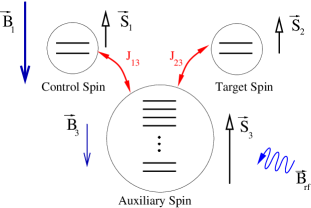
Figure 1: Three-spin system.

The Hamiltonian of the system is

$$\begin{array}[]{lll}H&=\vec{B}_{1}\vec{S}_{1}+\vec{B}_{3}\vec{S}_{3}-J_{13}\vec{S}_{1}\vec{S}_{3}-J_{23}\vec{S}_{2}\vec{S}_{3}&+\\ &&\\ &\frac{1}{2}B_{rf}{\{}e^{i\omega t}{S}_{3}^{+}+e^{-i\omega t}{S}_{3}^{-}{\}}.\\ \end{array}$$ (1)

Here we set $\gamma$ = 1 ($\gamma$ is the magnitude of the electron gyromagnetic ratio) and $\hbar=1$. The rf field rotates in the clockwise direction.

The parameters chosen for the computer simulations are:

$$\begin{array}[]{lll}J_{23}&=2,\quad J_{13}=20,\quad B_{3}=25,\quad B_{1}=2500,\quad B_{rf}=3,&\\ &&\\ S_{1}&=S_{2}=1/2,\quad S_{3}=51/2,\quad\omega=15.\end{array}$$ (2)

The duration $\tau$ of the action of the rf field corresponds to the $\pi$ pulse:

$$B_{rf}\tau=\pi.$$ (3)

The initial conditions describe an auxiliary spin $S_{3}$ and the target spin $S_{2}$ pointing “up” in the positive $z$-direction, while the control spin $S_{1}$ may point “up” (as shown in Fig. 1) or “down” (not shown in Fig. 1).

For our chosen parameters, the local magnetic field on the control spin $B_{1}=2500$ is much greater than the exchange field $J_{13}S_{3}$ = 510. So, one can expect that the direction of the control spin is determined by the local field. Next, for the auxiliary spin the local magnetic field $B_{3}$ = 25 is more than twice the exchange field $J_{13}S_{1}$ = 10 produced by the control spin and much greater than the exchange field $J_{23}S_{2}$ = 1 produced by the target spin. The rf field $B_{rf}$ =3 is greater than the exchange field produced by the target spin but smaller than the exchange field produced by the control spin. Thus, one can expect that the action of the rf pulse on the auxiliary spin depends on the direction of the control spin and does not depend on the direction of the target spin. If we ignore the influence of the target spin, the resonant frequency of the Larmor precession of the auxiliary spin is “35” for the control spin pointing “up” and “15” for the control spin pointing “down”. With $\omega$ = 15 the auxiliary spin changes its direction only if the control spin points “down”. Finally, the exchange field on the target spin $J_{23}S_{3}$ = 51 is much greater than the expected frequency of its oscillations: the transverse component of the exchange field is expected to oscillate with the frequency $\omega$ = 15, and the $z$-component with frequency $B_{rf}$ = 3. (The magnetic field has the same unit as the frequency, as we set $\gamma$ = 1.) Thus, our scheme is expected to implement a controlled change of the target spin state.

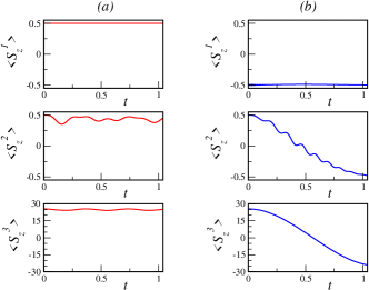
Figure 2: Average spin evolution: a) – for the control spin pointing “up”, and b) – for the control spin pointing “down”.

The Schrödinger equation for the wave function $|\psi(t)\rangle$ of three spins in the $S_{z}$ representation

$$|s_{1},s_{2},n\rangle,$$

with

$$s_{1}=\pm 1/2,\quad s_{2}=\pm 1/2,\quad n=1,\ldots,52,$$

can be written as a system of 104 coupled linear equations for the coefficients

$$C_{n}(t)=\langle s_{1},s_{2},n|\psi(t)\rangle,$$

$$\begin{array}[]{lll}\displaystyle i\frac{dC_{n}}{dt}&=B_{3}\left(\displaystyle\frac{53}{2}-n\right)C_{n}+&\\ &&\\ &\displaystyle\frac{1}{2}B_{rf}\ \sqrt{n(52-n)}\ e^{i\omega t}\ C_{n+1}+&\\ &&\\ &\sqrt{(n-1)(53-n)}\ e^{-i\omega t}\ C_{n-1}.\\ \end{array}$$ (4)

Here we have used the well known expressions for the matrix elements of the spin. In particular, for the auxiliary spin $S_{3}$ we have :

$$\begin{array}[]{lll}&\langle s_{1},s_{2},n|S_{3}^{z}|s_{1},s_{2},n\rangle=\displaystyle\frac{53}{2}-n,&\\ &&\\ &\langle s_{1},s_{2},n|S_{3}^{+}|s_{1},s_{2},n+1\rangle=\sqrt{n(52-n)},&\\ &&\\ &\langle s_{1},s_{2},n|S_{3}^{-}|s_{1},s_{2},n-1\rangle=\sqrt{n(52-n)}.&\\ &&\\ &&\end{array}$$ (5)

In Fig. 2 we show the results of our computer simulations, which confirm the expected dynamics of the spin system. Namely, if the control spin $S_{1}$ is initially “up”, the target spin $S_{2}$ does not change its state. (See Fig. 2a.) If the control spin $S_{1}$ is initially “down”, the target spin $S_{2}$ changes its state from “up” to “down”. (See Fig. 2b.) During this operation, both spins remain in their ground states.

In conclusion, we propose a scheme, which in effect relates adiabatic quantum computation with traditional gate quantum computation. Our scheme implements the change of state of the target spin controlled by the state of the control spin in such a way that that both spins remain in their ground states. This result is achieved using an auxiliary spin, which mediates the interaction between the control and target spins.

Note, that our operation can be considered as a two-bit digital logic gate $G$ which changes the state of the target bit if and only if it is different from the state of the control bit. We may implement this gate using a linear polarized rf field which is a superposition of two circularly polarized rf fields. Indeed, if we assign the value “0” to spin “up” and the value “1” to spin “down”, and request that all spins are initially in their ground states, we will get the transformation: $G(00)=(00)$, $G(10)=(11)$, $G(11)=(11)$, and $G(01)=(00)$. In future we plan to study the opportunities to implement quantum logic gates holding the qubits in their ground states.

The work by G. P. B. is supported by the NNSA of the U. S. DOE at LANL under Contract No. DE-AC52-06NA25396.

References

- (1) Arnab Das, Bikas Chakrabarti (Eds), Quantum Annealing and Other Optimization Methods, Lecture Notes in Physics, Springer, Heidelberg, 679, (2005).
- (2) W.M. Kaminsky and S. Lloyd, quant-ph/0211152 (2002).
- (3) E. Farhi, J. Goldstone, S. Gutmann, J. Lapan, A. Lundgren, and D. Preda, Science 292, 472 (2001).
- (4) R. Harris, A.J. Berkley, M.W. Johnson, P. Bunyk, S. Govorkov, M.C. Thom, S. Uchaikin, A.B. Wilson, J. Chung, E. Holtham, J.D. Biamonte, A.Yu. Smirnov, M.H.S. Amin, and Alec Maassen van den Brink, cond-mat/0608253, (2006).
- (5) G.P. Berman, G.D. Doolen, R. Mainieri, and V.I. Tsifrinovich, Introduction to Quantum Computers, World Scientific, Singapore-New Jersey-London-Hong Kong (1998).