Model-independent constraints on reionization from large-scale CMB polarization

Abstract

On large angular scales, the polarization of the CMB contains information about the evolution of the average ionization during the epoch of reionization. Interpretation of the polarization spectrum usually requires the assumption of a fixed functional form for the evolution, e.g. instantaneous reionization. We develop a model-independent method where a small set of principal components completely encapsulate the effects of reionization on the large-angle $E$-mode polarization for any reionization history within an adjustable range in redshift. Using Markov Chain Monte Carlo methods, we apply this approach to both the 3-year WMAP data and simulated future data. WMAP data constrain two principal components of the reionization history, approximately corresponding to the total optical depth and the difference between the contributions to the optical depth at high and low redshifts. The optical depth is consistent with the constraint found in previous analyses of WMAP data that assume instantaneous reionization, with only slightly larger uncertainty due to the expanded set of models. Using the principal component approach, WMAP data also place a 95% CL upper limit of 0.08 on the contribution to the optical depth from redshifts $z>20$. With improvements in polarization sensitivity and foreground modeling, approximately five of the principal components can ultimately be measured. Constraints on the principal components, which probe the entire reionization history, can test models of reionization, provide model-independent constraints on the optical depth, and detect signatures of high-redshift reionization.

1. Introduction

The amplitude of the $E$-mode component of the cosmic microwave background (CMB) polarization on large scales provides the current best constraint on the Thomson scattering optical depth to reionization, $\tau$. Using the first three years of data from the Wilkinson Microwave Anisotropy Probe (WMAP) and making the simple assumption that the universe was reionized instantaneously, Spergel et al. (2006) find $\tau=0.09\pm 0.03$. Theoretical studies suggest that the process of reionization was too complex to be well described as a sudden transition (e.g., Barkana & Loeb, 2001). Previous studies have examined how the constraint on $\tau$ depends on the evolution of the globally-averaged ionized fraction during reionization, $x_{e}(z)$, for a variety of specific theoretical scenarios. If the assumed form of $x_{e}(z)$ is incorrect, the estimated value of $\tau$ can be biased; this bias can be lessened by considering a wider variety of reionization histories at the expense of increasing the uncertainty in $\tau$ (Kaplinghat et al., 2003; Holder et al., 2003; Colombo et al., 2005).

The angular scales on which CMB polarization from reionization is correlated depend on the horizon size at the redshift of the free electrons: the higher the redshift, the higher the multipole, $\ell$ (e.g., Zaldarriaga, 1997; Hu & White, 1997). Varying $x_{e}(z)$ changes the relative contributions to the polarization coming from different redshifts, and therefore changes the shape of the large-scale $E$-mode angular power spectrum, $C_{\ell}^{EE}$. Because of this dependence, measurements of the low-$\ell$ $E$-mode spectrum should place at least weak constraints on the global reionization history in addition to the constraint on the total optical depth. Recent studies suggest that WMAP data provide little information about $x_{e}(z)$ beyond $\tau$ (e.g., Lewis et al., 2006), but it is worth asking what we can ultimately expect to learn about reionization from CMB polarization.

Hu & Holder (2003) proposed using a principal component decomposition of the ionization history to quantify the information contained in the large-scale $E$-mode polarization. The effect of any ionization history on the $E$-modes can be completely described by a small number of eigenmode parameters, unlike a direct discretization of $x_{e}(z)$ in redshift bins. Here we extend the methods of Hu & Holder (2003) using Markov Chain Monte Carlo techniques to find constraints on the principal components of $x_{e}(z)$ using both the 3-year WMAP observations and simulated future data.

Analytic studies and simulations indicate that reionization is an inhomogeneous process, and this inhomogeneity is expected to contribute to the small-scale CMB temperature and polarization anisotropies (e.g., Hu, 2000; Iliev et al., 2006; Mortonson & Hu, 2007; Doré et al., 2007). Here we focus on the large-scale $E$-modes only ($\ell\lesssim 100$) where such effects can be neglected, so we only consider the evolution of the globally-averaged ionized fraction as a function of redshift.

In the following section, we describe the principal component method for parameterizing the ionization history and show that the effects of $x_{e}(z)$ on large-scale $E$-mode polarization can be encapsulated in a small set of parameters. The method allows $x_{e}(z)$ to be a free function of redshift that is not bounded by physical considerations, so in § 3 we derive limits that can be placed on the model parameters to eliminate most of the unphysical models where $x_{e}>1$ or $x_{e}<0$. We outline several ways to apply the principal component approach to constrain the reionization history with large-scale $E$-mode data in § 4. Using Markov Chain Monte Carlo methods, we examine some of these applications in more detail in § 5 using both 3-year WMAP data and simulated future CMB polarization data. We summarize our findings and conclude in § 6.

2. Ionization History Eigenmodes

Models with similar total optical depth but different ionization histories can produce markedly different predictions for the $E$-mode power spectrum. In an instantaneous reionization scenario, the contribution to the optical depth from $x_{e}(z)$ is concentrated at the lowest redshifts possible for a given $\tau$, and the $E$-mode power spectrum for such a model is sharply peaked on large scales, at $\ell\lesssim 10$. The main effect of shifting some portion of the reionization history to higher redshifts while keeping $\tau$ fixed is to reduce the $E$-mode power on the largest scales and increase it on smaller scales.

This redistribution of power is illustrated in Figure 1 by the ionization histories and $C_{\ell}^{EE}$ for two models, one with nearly instantaneous reionization and the other with comparable optical depth but with $x_{e}(z)$ concentrated at higher $z$. In general, a flatter large-scale $E$-mode spectrum with power extending out to $\ell\sim 10$-20 is a sign of a large ionized fraction at high redshift. However, there is not a one-to-one correspondence between $\ell$ and $z$; the ionized fraction within any particular narrow redshift bin affects $C_{\ell}^{EE}$ over a wide range of angular scales. Ionized fractions in adjacent redshift bins have highly correlated effects on $C_{\ell}^{EE}$, which makes it difficult to extract from $E$-mode polarization data a constraint on $x_{e}$ at a specific redshift.

Figure 1.— $E$-mode polarization angular power spectra and ionization histories (inset) for a nearly-instantaneous reionization model with optical depth $\tau=0.105$ (thick curves) and an extended, “double” reionization history with $\tau=0.090$ (thin). Points with error bars represent the 3-year WMAP data from Page et al. (2006).

As suggested by Hu & Holder (2003), one can use principal components of the reionization history as the model parameters instead of $x_{e}$ in redshift bins. These components are defined to have uncorrelated contributions to the $E$-mode power; since each has a unique effect on $C_{\ell}^{EE}$, the amplitudes of the components can be inferred from measurements of the large-scale power spectrum. Principal component analysis of $x_{e}(z)$ also indicates which components can be determined best from the data. In this section, we describe the principal component method and introduce the notation that we will use throughout the paper.

Consider a binned ionization history $x_{e}(z_{i})$, $i\in\{1,2,\ldots,N_{z}\}$, with redshift bins of width $\Delta z$ spanning $z_{\rm min}\leq z\leq z_{\rm max}$, where $z_{1}=z_{\rm min}+\Delta z$ and $z_{N_{z}}=z_{\rm max}-\Delta z$ so that $N_{z}+1=(z_{\rm max}-z_{\rm min})/\Delta z$. Throughout this paper we assume that the ionized fraction is $x_{e}\approx 1$ for redshifts $z\leq z_{\rm min}$ and $x_{e}\approx 0$ at $z\geq z_{\rm max}$. We take $z_{\rm min}=6$, consistent with observations of quasar spectra (Fan et al., 2006).

The principal components of $x_{e}(z_{i})$ are eigenfunctions of the Fisher matrix, computed by taking derivatives of $C_{\ell}^{EE}$ with respect to $x_{e}(z_{i})$:

$$F_{ij}=\sum_{\ell=2}^{\ell_{\rm max}}\left(\ell+\frac{1}{2}\right)\frac{\partial\ln C_{\ell}^{EE}}{\partial x_{e}(z_{i})}\frac{\partial\ln C_{\ell}^{EE}}{\partial x_{e}(z_{j})}\,,$$ (1)

assuming full sky coverage and neglecting noise. Since $x_{e}(z_{i})$ only significantly contributes to the $E$-mode spectrum at small $\ell$, we typically truncate the sum in equation (1) at $\ell_{\rm max}=100$ where $C_{\ell}^{EE}$ is dominated by the first acoustic peak. The derivatives are evaluated at a fiducial reionization history, $x_{e}^{\rm fid}(z_{i})$. Following Hu & Holder (2003) we typically choose $x_{e}^{\rm fid}(z_{i})$ to be constant during reionization, although other functional forms may be used.

Since the effects on $C_{\ell}^{EE}$ of $x_{e}(z_{i})$ in adjacent redshift bins are highly correlated, the Fisher matrix contains large off-diagonal elements. The principal components $S_{\mu}(z_{i})$ are the eigenfunctions of $F_{ij}$,

$$F_{ij}=(N_{z}+1)^{-2}\sum_{\mu=1}^{N_{z}}S_{\mu}(z_{i})\sigma^{-2}_{\mu}S_{\mu}(z_{j}),$$ (2)

where the factor $(N_{z}+1)^{-2}$ is included so that the eigenfunctions and their amplitudes have certain convenient properties. The inverse eigenvalues, $\sigma^{2}_{\mu}$, give the estimated variance of each principal component eigenmode from the measurement of low-$\ell$ $E$-modes. We order the modes so that the best-constrained principal components (smallest $\sigma^{2}_{\mu}$) have the lowest values of $\mu$, starting at $\mu=1$. The noise level and other characteristics of an experiment can be included in the construction of the eigenfunctions, but since the effect on $S_{\mu}(z)$ is small we always use the noise-free eigenfunctions here.

The eigenfunctions satisfy the orthogonality and completeness relations

$$\int_{z_{\rm min}}^{z_{\rm max}}dz~{}S_{\mu}(z)S_{\nu}(z) = (z_{\rm max}-z_{\rm min})\delta_{\mu\nu}\,,$$ (3)

$$\sum_{\mu=1}^{N_{z}}S_{\mu}(z_{i})S_{\mu}(z_{j}) = (N_{z}+1)\delta_{ij}\,.$$ (4)

The normalization of $S_{\mu}(z)$ is chosen so that the eigenfunctions are independent of bin width as $\Delta z\rightarrow 0$. In equation (3) and elsewhere in this paper where there are sums over redshift, we assume the continuous limit, replacing $\sum_{i}\Delta z$ by $\int dz$. As long as the bin width is chosen to be sufficiently small, the final results we obtain are independent of the redshift binning. We adopt $\Delta z=0.25$ as the default bin width.

The three lowest-variance eigenfunctions for two different fiducial models are shown in Figure 2. The lowest eigenmode ($\mu=1$) is an average of the ionized fraction over the entire redshift range, weighted at high $z$. The $\mu=2$ mode can be thought of as a difference between the amount of ionization at high $z$ and at low $z$, and higher modes follow this pattern with weighted averages of $x_{e}(z)$ that oscillate with higher and higher frequency in redshift. Eigenfunctions of fiducial models with different values of $z_{\rm max}$ have similar shapes with the redshift axis rescaled according to the width of $(z_{\rm max}-z_{\rm min})$. The eigenfunctions are mostly insensitive to the choice of ionized fraction in the constant-$x_{e}$ fiducial histories.

Figure 2.— Eigenfunctions for fiducial models with $z_{\rm max}=30$ and constant $x_{e}=0.15$ (top), and $z_{\rm max}=20$ and $x_{e}=0.3$ (bottom). In each case, the first three modes are shown: $\mu=1$ (thick), 2 (medium) and 3 (thin). For both fiducial models, $z_{\rm min}=6$ and $\Delta z=0.25$.

An arbitrary reionization history can be represented in terms of the eigenfunctions as

$$x_{e}(z)=x_{e}^{\rm fid}(z)+\sum_{\mu}m_{\mu}S_{\mu}(z),$$ (5)

where the amplitude of eigenmode $\mu$ for a perturbation $\delta x_{e}(z)\equiv x_{e}(z)-x_{e}^{\rm fid}(z)$ is

$$m_{\mu}=\frac{1}{z_{\rm max}-z_{\rm min}}\int_{z_{\rm min}}^{z_{\rm max}}dz~{}S_{\mu}(z)\delta x_{e}(z).$$ (6)

[Note that our conventions for the normalization of $m_{\mu}$ and $S_{\mu}(z)$ differ from those of Hu & Holder (2003) by factors of $(N_{z}+1)^{1/2}$.] Any global ionization history $x_{e}(z)$ over the range $z_{\rm min}<z<z_{\rm max}$ is completely specified by a set of mode amplitudes $m_{\mu}$.

If perturbations to the fiducial history are small, $\delta x_{e}(z)\ll 1$, then the mode amplitudes are uncorrelated, with covariance matrix $\langle m_{\mu}m_{\nu}\rangle=\sigma_{\mu}^{2}\delta_{\mu\nu}$. For a fixed fiducial model, however, arbitrary reionization histories generally have $\delta x_{e}\sim 1$, in which case the amplitudes of different modes can become correlated as we discuss in § 5.3.

The main advantage of using the principal component eigenmodes of $x_{e}(z)$ instead of some other parameterization is that most of the information relevant for large-scale $E$-modes is contained in the first few modes. This means that if one constructs $x_{e}(z)$ from equation (5) keeping only the first few terms in the sum over $\mu$, then the $E$-mode spectrum of the resulting ionization history will closely match that of $x_{e}(z)$ with all modes included in the sum. The effect of each eigenmode on $C_{\ell}^{EE}$ becomes smaller as $\mu$ increases, as shown in Figure 3 for the first two modes. Hu & Holder (2003) demonstrated that for a specific fiducial ionization history $x_{e}^{\rm fid}(z)$ and assumed true history, only the first three modes of $x_{e}(z)$ are needed to produce $C_{\ell}^{EE}$ indistinguishable from the true $E$-mode spectrum.

Figure 3.— Change in $\ln C_{\ell}^{EE}$ per unit $m_{\mu}$ for fiducial $x_{e}(z)$ with $z_{\rm max}=30$ (solid) and 20 (dashed), showing the effect on $C_{\ell}^{EE}$ of the first two principal components, $\mu=1$ (thick) and $2$ (thin).

The ionization histories and corresponding $E$-mode spectra in Figure 4 demonstrate this completeness for a fairly extreme model in which the first ten eigenmodes all have significant amplitudes. Even in the simplest case where a single eigenmode is used in place of the original $x_{e}(z)$, the error in $C_{\ell}^{EE}$ is only $\sim 10\%$. With 3-5 modes, the error is a few percent or less at all multipoles and safely smaller than the cosmic variance of

$${\Delta C_{\ell}^{EE}\over C_{\ell}^{EE}}=\sqrt{2\over 2\ell+1}\,.$$ (7)

The top panel of Figure 4 shows that this completeness does not extend to the ionization history itself: $x_{e}(z)$ constructed from as many as five eigenmodes is a poor approximation to the full reionization history.

Figure 4.— Test of completeness in $C_{\ell}^{EE}$ for ionization histories with truncated sets of eigenfunctions. The base history (top panel, dashed) is the sum of the first 10 eigenfunctions with comparable values of $|m_{\mu}|$ for each mode. Solid curves show $x_{e}(z)$ (top) and the error in $C_{\ell}^{EE}$ (bottom) for histories that retain the first one (thin curves), three (medium), and five (thick) eigenmodes. The fiducial model used for the eigenmode decomposition has constant $x_{e}=0.15$ from $z_{\rm min}=6$ up to $z_{\rm max}=30$.

From this and other similar tests on the completeness in $C_{\ell}^{EE}$ of the lowest-variance eigenmodes we conclude that the first 3-5 modes contain essentially all of the information about the reionization history that is relevant for large-scale $E$-mode polarization. This fact is particularly useful for constraining the global reionization history with CMB polarization data using Markov Chain Monte Carlo techniques. Since the number of parameters that must be added to a Monte Carlo chain to describe an arbitrary $x_{e}(z)$ is relatively small, we can obtain constraints from the data that are independent of assumptions about the reionization history with minimal added computational expense (Hu & Holder, 2003). The exact number of modes required varies depending on the true ionization history and the fiducial history, so when analyzing data it is a good idea to check that the results do not change significantly when the next modes are included in the sum in equation (5).

The main caveat to this model independence is that in practice we must set some maximum redshift for histories in any particular chain of Monte Carlo samples, ignoring any contribution to the observed low-$\ell$ $C_{\ell}^{EE}$ from ionization at $z>z_{\rm max}$. Since the eigenfunctions of the ionization history are stretched in redshift as $z_{\rm max}$ increases (Fig. 2), at higher $z_{\rm max}$ more modes are needed to accurately represent any particular feature in $x_{e}(z)$. For example, take the true ionization history to be instantaneous reionization at $z=11.5$. Figure 5 shows the error in $C_{\ell}^{EE}$ if we truncate the eigenmode sum of equation (5) at $N$ modes using fiducial histories with $z_{\rm max}=30$ and $z_{\rm max}=20$. For each fiducial model, the error decreases as the number of modes in the sum increases, but the error at fixed $N$ is larger for $z_{\rm max}=30$ than $z_{\rm max}=20$. The requirement of retaining a larger set of parameters as $z_{\rm max}$ increases makes it less practical to study models with significant reionization at extremely high redshifts [$z_{\rm max}\gtrsim 100$; e.g., Naselsky & Chiang (2004); Kasuya et al. (2004)], but even for $z_{\rm max}$ as high as $\sim 40$ the number of eigenmodes needed is reasonably small ($N\lesssim 5$).

Figure 5.— Error in $C_{\ell}^{EE}$ from $x_{e}(z)$ constructed from the first $N$ eigenmodes of fiducial models with $z_{\rm max}=30$ (solid curves) and 20 (dashed), taking $N=3$ (thin) and $N=5$ (thick). The true $x_{e}(z)$ and $C_{\ell}^{EE}$ are assumed to be those of an instantaneous reionization model with $\tau=0.09$.

While theories of reionization provide useful priors on $z_{\rm max}$ in the context of specific models, it would be better to be able to constrain $z_{\rm max}$ empirically by measuring the $E$-mode power accurately up to $\ell\sim 100$. The current 3-year WMAP polarization data have high enough signal-to-noise to be useful for parameter constraints only at $\ell<24$ (Page et al., 2006), so their sensitivity to high-$z$ reionization is limited. Given that ionization at some redshift generates polarization out to a maximum $\ell$, WMAP data can still place weak bounds on the total optical depth contribution above a certain redshift, even if it cannot distinguish whether these contributions arise from redshifts above a chosen $z_{\rm max}$ as we discuss in § 5.1. The values we choose here for $z_{\rm max}$ are partly influenced by the fact that few theoretical reionization scenarios predict an ionized fraction at $z\gtrsim 30$ that would significantly affect large-scale $C_{\ell}^{EE}$. Future data should better constrain $C_{\ell}^{EE}$ at higher multipoles, allowing useful limits to be placed on $z_{\rm max}$ from the data alone.

The need to consider a limited range in redshift is shared by other methods, for example those that constrain binned $x_{e}(z_{i})$ instead of the eigenmode amplitudes (Lewis et al., 2006). As already mentioned, the principal component approach has the unique advantages that results can be made independent of bin width and that relatively few extra parameters are required. However, this approach also has a unique difficulty in that the physicality of the reionization history [$0\leq x_{e}(z)\leq 1$] is not built in to the method. Hence constraints derived from measurements of the eigenmodes can be weaker than those from a method that enforces physicality. We can, however, place some prior constraints on the set of eigenmode amplitudes that must be satisfied by any physical model, as we discuss in the next section.

3. Priors from Physicality

Although the actual ionized fraction must be between 0 and 1 (neglecting helium reionization and the small residual ionized fraction after recombination), there is nothing in the construction of $x_{e}(z)$ from the eigenmodes in equation (5) that ensures that the ionized fraction will obey these limits. Whether or not $x_{e}$ has a physical value at a particular redshift depends on the amplitudes of all of the principal components. Even for a physical ionization history, the truncated sum up to mode $N$,

$$x_{e}^{(N)}(z)\equiv x_{e}^{\rm fid}(z)+\sum_{\mu=1}^{N}m_{\mu}S_{\mu}(z),$$ (8)

is not necessarily bounded by 0 and 1 at all redshifts. While formally it is possible to evaluate $C_{\ell}^{EE}$ for reionization histories with unphysical values of $x_{e}$, we would like to eliminate as much as possible those models for which the full sum of the eigenmodes, $x_{e}(z)=\lim_{N\to\infty}x_{e}^{(N)}(z)$, is unphysical.

We find the largest and smallest values of $m_{\mu}$ that are consistent with $x_{e}(z)\in[0,1]$ for all $z$ using the definition of $m_{\mu}$ in equation (6). We are free to choose $x_{e}^{\rm fid}(z)\in[0,1]$ so that $-x_{e}^{\rm fid}(z)\leq\delta x_{e}(z)\leq 1-x_{e}^{\rm fid}(z)$, where the lower limit is strictly negative or zero and the upper limit is positive or zero. For a particular mode $\mu$, the choice of $\delta x_{e}(z)$ that maximizes $m_{\mu}$ is

$$\delta x_{e}^{\rm max}(z)=\left\{\begin{array}[]{rl}-x_{e}^{\rm fid}(z),&S_{\mu}(z)\leq 0\\ 1-x_{e}^{\rm fid}(z),&S_{\mu}(z)>0.\end{array}\right.$$ (9)

Using this in equation (6) gives an upper limit on $m_{\mu}$. Similarly, a lower limit can be obtained by reversing the signs of the inequalities in equation (9). The resulting physicality bounds are $m_{\mu}^{(-)}\leq m_{\mu}\leq m_{\mu}^{(+)}$, where

$$m_{\mu}^{(\pm)}=\int_{z_{\rm min}}^{z_{\rm max}}dz\frac{S_{\mu}(z)[1-2x_{e}^{\rm fid}(z)]\pm|S_{\mu}(z)|}{2(z_{\rm max}-z_{\rm min})}.$$ (10)

If $m_{\mu}$ violates these bounds for any $\mu$, the reionization history is guaranteed to be unphysical for some range in redshift. The opposite is not true, however: even if all $m_{\mu}$ satisfy equation (10), $x_{e}(z)$ may still be unphysical for some $z$.

The parameter space that physical models may occupy is restricted further by an inequality that must be satisfied by all eigenmodes simultaneously. Assume for simplicity that the fiducial model has a constant ionized fraction, $x_{e}^{\rm fid}\in[0,1]$, for $z_{\rm min}<z<z_{\rm max}$. Any physical reionization history $x_{e}(z)$ must satisfy

$$\int_{z_{\rm min}}^{z_{\rm max}}dz[x_{e}(z)-x_{e}^{\rm fid}]^{2}\leq(z_{\rm max}-z_{\rm min})f,$$ (11)

where $f\equiv\max[(x_{e}^{\rm fid})^{2},(1-x_{e}^{\rm fid})^{2}]$. Using equation (5), the left side of the inequality can also be written

$$\int_{z_{\rm min}}^{z_{\rm max}}dz[x_{e}(z)-x_{e}^{\rm fid}]^{2} = \int_{z_{\rm min}}^{z_{\rm max}}dz\left[\sum_{\mu}m_{\mu}S_{\mu}(z)\right]^{2}$$ (12)

$$= (z_{\rm max}-z_{\rm min})\sum_{\mu}m_{\mu}^{2}\,,$$

where the second line follows from the orthogonality of the eigenfunctions (eq. [3]). Comparing equations (11) and (12) we obtain a constraint on the sum of the squares of the mode amplitudes,

$$\sum_{\mu}m_{\mu}^{2}\leq f,$$ (13)

where $0.25\leq f\leq 1$, depending on the value of $x_{e}^{\rm fid}$. As with the physicality bounds of equation (10), this upper limit is a necessary but not sufficient condition for physicality.

Since in practice we can only constrain a limited set of eigenmodes, the uncertainty in modes higher than the first few prevents us from simply excluding all models where $x_{e}<0$ or $x_{e}>1$ at any redshift because the higher modes can have a significant effect on $x_{e}(z)$. However, as shown in § 2, the higher modes do not affect the polarization power spectrum since the high-frequency oscillations in redshift of higher modes are averaged out. Similarly, such eigenmodes have a small effect on the optical depth from a sufficiently large range in redshift. For example, the optical depth from $15<z<30$ due to modes $\mu>5$ subject to the physicality constraints of this section can be no larger than $\sim 0.01$, and is likely to be smaller for realistic reionization scenarios. Because of this, we assume that we can place priors on the optical depth that correspond to $0\leq x_{e}\leq 1$ over the relevant range in redshift. Reionization histories with an unphysical optical depth over a large range in redshift are considered to be unphysical models since the addition of higher modes can not perturb the optical depth enough to give it a physical value.

4. Applications of the Principal Component Method

Once constraints on the principal components of the reionization history have been obtained from CMB polarization data, there are several ways to use those constraints to place limits on observables such as $\tau$ or to test theories of reionization (Hu & Holder, 2003). We describe some possible applications in this section, and in § 5 we put these ideas into practice using the 3-year WMAP data and simulated future data.

As mentioned in § 1, the constraint on the total optical depth to reionization depends on the assumed model for $x_{e}(z)$. The principal component method allows us to explore all globally-averaged ionization histories within a chosen redshift range, $z_{\rm min}<z<z_{\rm max}$. For a given set of eigenmode amplitudes, $\{m_{\mu}\}$, equation (5) yields the corresponding ionization history which can then be integrated to find the optical depth between any two redshifts $z_{1}$ and $z_{2}$,

$$\tau(z_{1},z_{2})=0.0691(1-Y_{p})\Omega_{b}h\int_{z_{1}}^{z_{2}}dz\frac{(1+z)^{2}}{H(z)/H_{0}}x_{e}(z).$$ (14)

In particular, the total optical depth to reionization is

$$\tau=\tau(0,z_{\rm min})+\tau(z_{\rm min},z_{\rm max}),$$ (15)

where $\tau(0,z_{\rm min})\approx 0.04$ for $z_{\rm min}=6$. The principal component approach provides a model-independent way to constrain $\tau$, so we expect the results to be unbiased and the uncertainty in $\tau$ to accurately reflect the present uncertainty about $x_{e}(z)$. Moreover, the information about $\tau(z_{\rm min},z_{\rm max})$ is encapsulated in the first few eigenmodes, i.e. the truncated ionization history of equation (8), $x_{e}^{(N)}(z)$, with $N=3$-5 for typical fiducial models.

The total optical depth and the first principal component amplitude, $m_{1}$, are similar quantities in that they are both averages of $x_{e}(z)$ weighted at high $z$. As we show in the next section, CMB $E$-mode polarization data can constrain higher eigenmodes as well ($\mu\geq 2$). In particular, the second mode should be the next best constrained quantity since it is constructed to have the smallest variance after $m_{1}$. Since $m_{2}$ is related to the difference in $x_{e}$ between high redshift and low redshift (see Fig. 2), we might guess that besides total $\tau$ the data are mainly constraining the fraction of optical depth coming from high redshift versus low redshift. Given any set of mode amplitudes defining an ionization history, we can compute a low-$z$ optical depth, $\tau(z_{\rm min},z_{\rm mid})$, and a high-$z$ optical depth, $\tau(z_{\rm mid},z_{\rm max})$, for some choice of intermediate redshift, $z_{\rm mid}$.

Note that if either of the redshift ranges $[z_{\rm min},z_{\rm mid}]$ or $[z_{\rm mid},z_{\rm max}]$ is too narrow, constraints on the partial optical depths will be influenced by the physicality priors (since $0\leq x_{e}\leq 1$ sets limits on $\tau$ in redshift intervals as discussed in § 3) and by the uncertainty in modes higher than those included in the chain, which have greater effect on the optical depth in narrower redshift intervals. For these reasons, $z_{\rm mid}$ should be chosen to be not too close to either $z_{\rm min}$ or $z_{\rm max}$.

Given an appropriately chosen value of $z_{\rm mid}$, constraints on the principal components can be converted into constraints on the optical depths at high and low redshift. These partial optical depths are observables in the sense that high-$z$ and low-$z$ optical depth affect the large-scale $E$-modes over different ranges of multipoles. For example, compare the two reionization models in Figure 1. Both have similar total optical depth, but in one case $\tau$ only comes from $z<15$, resulting in more power at $\ell<8$ and less power at $\ell>8$ than the other model in which the optical depth primarily comes from $z>15$.

Besides learning about the relative amount of ionization at $z<z_{\rm mid}$ and $z>z_{\rm mid}$, the partial optical depth constraints also provide a way to empirically set the maximum redshift, $z_{\rm max}$. If some set of data are found to place a tight upper bound on $\tau(z_{\rm mid},z_{\rm max})$ for fairly conservative (i.e. large) values of $z_{\rm mid}$ and $z_{\rm max}$, then for analyses of future data this value of $z_{\rm mid}$ can be used as a new, lower value for $z_{\rm max}$ since optical depth from higher redshifts is small. This approach assumes that there is essentially no reionization earlier than the original $z_{\rm max}$, but as long as this initial maximum redshift is taken to be large the presence or absence of high-$z$ ionization can be tested in this way over a wide range of redshifts. We explore this idea further in § 5.

While we do not examine constraints on specific reionization models in this paper, the principal component approach is well suited to model testing. Consider a model of the global reionization history, $x_{e}(z;\bm{\theta})$, parameterized by $\bm{\theta}$. This could be a simple toy model (for example, instantaneous reionization where $\bm{\theta}$ is a single parameter, the redshift of reionization) or a more physical model where $\bm{\theta}$ might include parameters that govern properties of the ionizing sources. For a particular choice of $x_{e}^{\rm fid}(z)$, the principal component amplitudes of the reionization model follow from equation (6), giving a set of mode amplitudes that depend on the model parameters, $\{m_{\mu}(\bm{\theta})\}$. Then constraints on the mode amplitudes from CMB polarization data (defined using the same fiducial history) can be mapped to constraints on the parameters of the reionization model.

Applying this method to a model that has as one of its parameters a maximum redshift allows one to obtain constraints on $z_{\rm max}$ within a class of theoretical models. Although obtaining good constraints on model parameters does not necessarily imply validation of the model class, this procedure provides a straightforward method by which different model classes can tested and falsified within a single analysis.

Generating Monte Carlo chains to find constraints on $\{m_{\mu}\}$ as described in the next section can be a somewhat time-consuming process, but it only needs to be done once per redshift range, after which any model of the global reionization history within this range $z_{\rm min}<z<z_{\rm max}$ can be tested using the same parameter chains. In cases where constraints from the data turn out to be close to Gaussian, the covariance matrix of the principal components can be used in place of the full Monte Carlo chains, reducing the amount of information needed for model testing from $\sim 10^{5}$ numbers in chains of Monte Carlo samples to only $N(N+3)/2$ numbers when $N$ eigenmodes are included in the chains [$N$ mean values plus $N(N+1)/2$ entries in the covariance matrix, $\langle m_{\mu}m_{\nu}\rangle$]. However, near-Gaussian constraints on $\{m_{\mu}\}$ are likely to be possible only for certain realizations of future data, as discussed in the next section.

5. Markov Chain Monte Carlo Constraints on Eigenmodes

We find reionization constraints from CMB polarization data using Markov Chain Monte Carlo (MCMC) techniques to explore the principal component parameter space (see e.g. Christensen et al., 2001; Kosowsky et al., 2002; Dunkley et al., 2005). Chains of Monte Carlo samples are generated using the publicly available code CosmoMC (Lewis & Bridle, 2002), which includes the code CAMB (Lewis et al., 2000) for computing the theoretical angular power spectrum at each point in the $\{m_{1},\ldots,m_{N}\}$ parameter space. We have modified both codes to allow specification of an arbitrary reionization history calculated from a set of mode amplitudes using equation (5).

The principal component amplitudes are the only parameters allowed to vary in the chains. Since nearly all the information in $C_{\ell}^{EE}$ from reionization is contained within the first few eigenmodes of $x_{e}(z)$, we include the modes $\{m_{1},\ldots,m_{N}\}$ in each chain with $3\leq N\leq 5$. We use only the $E$-mode polarization data for parameter constraints, and assume that the values of the standard $\Lambda$CDM parameters (besides $\tau$) are fixed by measurements of the CMB temperature anisotropies. This leads to a slight underestimate of the error on $\tau$ as we discuss later, but to a good approximation the effect of $x_{e}(z)$ on the large-scale $E$-modes is independent of the other parameters.

Specifically, we take $\Omega_{b}h^{2}=0.0222$, $\Omega_{c}h^{2}=0.106$, $100\theta=1.04$ (corresponding to $h=0.73$), $A_{s}e^{-2\tau}=1.7\times 10^{-9}$, and $n_{s}=0.96$, consistent with results from the most recent version of the WMAP 3-year likelihood code. When computing the optical depth to reionization we take the primordial helium fraction to be $Y_{p}=0.24$. We also assume that $z_{\rm min}=6$, so that the optical depth contributed at lower redshifts is fixed at $\tau(z_{\rm min})\approx 0.04$. The remaining total optical depth from reionization, $\tau(z_{\rm min},z_{\rm max})$, is determined by the values of $\{m_{\mu}\}$ for each sample in the chains. The default bin width for our fiducial models $x_{e}^{\rm fid}(z)$ is $\Delta z=0.25$, which is small enough that numerical effects related to binning should be negligible.

To get accurate results from MCMC analysis, it is important to make sure that the parameter chains contain enough independent samples covering a sufficient volume of parameter space so that the density of the samples converges to the actual posterior probability distribution. For each scenario that we study, we run 4 separate chains until the Gelman and Rubin convergence statistic $R$, corresponding to the ratio of the variance of parameters between chains to the variance within each chain, satisfies $R-1<0.01$ (Gelman & Rubin, 1992; Brooks & Gelman, 1998). The convergence diagnostic of Raftery & Lewis (1992) is used to determine how much each chain must be thinned to obtain independent samples. Both of these statistics and other diagnostic measures are computed automatically by CosmoMC.

Since $x_{e}(z)$ during reionization must match onto $x_{e}\approx 1$ at $z=z_{\rm min}$ and $x_{e}\approx 0$ at $z=z_{\rm max}$, there are often sharp transitions at these redshifts since nothing in equation (5) forces $x_{e}(z)$ to satisfy these boundary conditions. To avoid problems with the time integration in CAMB, we smooth the reionization history by convolving $x_{e}(z)$ with a Gaussian of width $\sigma_{z}=0.5$.

As described in previous sections, we assume that $0\leq x_{e}\leq 1$ between $z_{\rm min}$ and $z_{\rm max}$. This assumption neglects helium reionization, which can make $x_{e}$ slightly larger than unity, and the small residual ionized fraction remaining after recombination that prevents $x_{e}$ from ever being exactly zero. These are relatively small effects, especially since we are not placing constraints on $x_{e}(z)$ directly but rather on weighted averages of $x_{e}$ over redshift. The residual ionized fraction at $z>z_{\rm max}$ is accounted for in the Monte Carlo exploration of reionization histories.

In § 5.1, we examine the current constraints from the 3-year WMAP data. We then provide forecasts for principal component constraints with idealized, cosmic variance-limited, simulated data in § 5.2. In each case the likelihood computation includes only the $E$-mode polarization data, up to $\ell=100$ for simulated data and $\ell=23$ for WMAP; the likelihood code for WMAP does not use $C_{\ell}^{EE}$ at smaller scales due to low signal-to-noise. At multipoles $\ell\gtrsim 100$ the global reionization history only affects the amplitude of the angular power spectra, which we fix by setting $A_{s}e^{-2\tau}$ constant in the Monte Carlo chains. A comparison of the MCMC results with the Fisher matrix approximation follows in § 5.3.

5.1. Constraints from WMAP

In our analysis of WMAP data we use the 3-year WMAP likelihood code, with settings chosen so that likelihoods include only contributions from the low-$\ell$ $E$-mode polarization. In this regime, the code computes model likelihoods with a pixel-based method instead of using the angular power spectrum (Page et al., 2006). Since the maximum redshift at which there is still a significant ionized fraction is uncertain, we generate Monte Carlo chains using different fiducial models with $10\leq z_{\rm max}\leq 40$. To avoid possible bias due to neglecting the possibility of high-redshift reionization, we focus here on the results obtained using the more conservative values of $z_{\rm max}=30$ and 40.

The MCMC constraints on the first three principal components from WMAP are shown in Figure 6 using fiducial models with $z_{\rm max}=30$ and $z_{\rm max}=40$. The marginalized constraints are plotted within the physicality bounds of equation (10), $m_{\mu}^{(-)}\leq m_{\mu}\leq m_{\mu}^{(+)}$, so the size of the contours inside each box gives an idea of the constraining power of the data within the space of potentially physical models. For both fiducial histories, the data place a strong upper limit on $m_{1}$ and weakly constrain $m_{2}$. It is important to note that although the parameters $\{m_{1},m_{2},m_{3}\}$ have the same names in both the $z_{\rm max}=30$ and $z_{\rm max}=40$ plots, they are defined with respect to different fiducial models and so we do not expect the contours in the left and right plots in Figure 6 to agree exactly. The qualitative similarity between the contours simply reflects the fact that the eigenfunctions for different $z_{\rm max}$ have similar shapes (Figure 2).

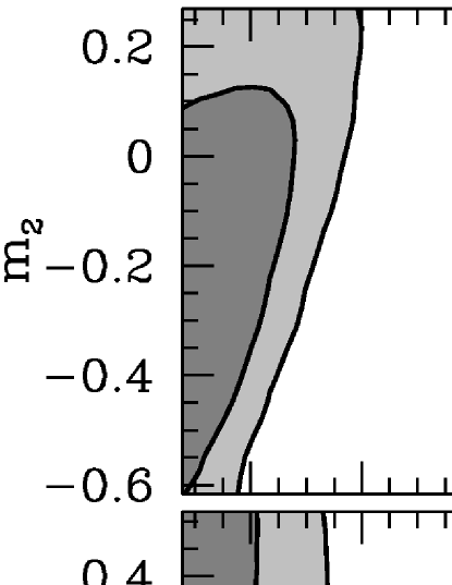
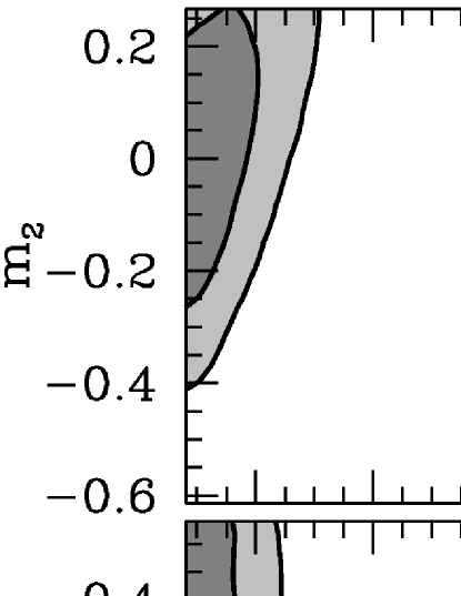
Figure 6.— Marginalized 2D contours (dark shading: 68% CL; light: 95%) for the first three principal components of $x_{e}(z)$ from MCMC analysis of 3-year WMAP $E$-mode polarization data, using fiducial reionization histories with $z_{\rm max}=30$ (left) and $z_{\rm max}=40$ (right). Note that the mode amplitudes $m_{\mu}$ are defined differently in the left and right panels since the fiducial models are different.

Since $m_{1}$ and $\tau$ are both averages of $x_{e}$ from $z_{\rm min}$ to $z_{\rm max}$ with more weight at high $z$ than low $z$, the strong constraint on $m_{1}$ mostly reflects the ability of the data to constrain the total optical depth to reionization. Indeed, $m_{1}$ and $\tau$ are strongly correlated in the Monte Carlo chains, while the correlations between $\tau$ and higher principal components of $x_{e}(z)$ are weaker.

Relative to the physicality bounds, the constraints in Figure 6 are stronger for the $z_{\rm max}=40$ chains than for $z_{\rm max}=30$; this is to be expected since the physicality bounds on $\{m_{\mu}\}$ permit a greater variety of ionization histories, and in particular a wider range in $\tau$, when $z_{\rm max}$ is larger. The range of eigenmode amplitudes allowed by the limits of equation (10) is nearly independent of $z_{\rm max}$, but the effect of a unit-amplitude principal component on $C_{\ell}^{EE}$ increases with $z_{\rm max}$ as illustrated in Figure 3.

As described in § 4, principal component constraints from MCMC yield model-independent constraints on the total optical depth. For each Monte Carlo sample of the principal components we compute $\tau$ using equation (15). The constraints on $\tau$ are listed in Table 1 for various values of $z_{\rm max}$ and $N$, the number of modes in the Monte Carlo chains. The uncertainty in $\tau$ from the Monte Carlo chains is slightly underestimated because we fix all cosmological parameters that are not directly related to reionization. To estimate the effect of this assumption, we compare constraints on $\tau$ in two cases where instantaneous reionization is assumed instead of using the model-independent principal component approach: one in which the non-reionization parameters are fixed as in the rest of our Monte Carlo chains, and the other, from the 3-year WMAP analysis of Spergel et al. (2006), in which these parameters are allowed to vary. These constraints, listed in rows 4 and 5 of Table 1, suggest that fixing $\Lambda$CDM parameters besides $\tau$ reduces $\sigma_{\tau}$ by $\sim 10\%$.

Table 1Constraints on total optical depth to reionization.

	Use PCs			Fix other
Data	of $x_{e}(z)$?	$z_{\rm max}$	$N$	parameters?	$\tau$
WMAP3	Yes	20	3	Yes	$0.098\pm 0.025$
WMAP3	Yes	30	5	Yes	$0.106\pm 0.027$
WMAP3	Yes	40	5	Yes	$0.107\pm 0.029$
WMAP3	No	–	–	Yes	$0.096\pm 0.027$
WMAP3	No	–	–	No	$0.089\pm 0.030$
CV	Yes	20	3	Yes	$0.103\pm 0.004$
CV	Yes	30	5	Yes	$0.108\pm 0.005$
CV	No	–	–	Yes	$0.108\pm 0.003$

Figure 7.— Left panel: Marginalized 2D contours (68 and 95%) from a $z_{\rm max}=30$ WMAP chain of Monte Carlo samples (thick curves), lines of constant $\tau=\{0.06,0.09,0.12\}$ (dashed lines), and the set of one-parameter instantaneous reionization models (thin curve) plotted in the $m_{1}-m_{2}$ plane. Higher eigenmodes ($\mu\geq 3$), which only weakly influence $\tau$, are fixed to $m_{\mu}=0$ for the purposes of plotting the constant-$\tau$ lines. Right panel: posterior probability of the optical depth from 3-year WMAP data, $P(\tau)$, for arbitrary $x_{e}(z)$ with $z_{\rm min}=6$, $z_{\rm max}=30$, and $N=5$ principal components (thick curve), and for the one-parameter instantaneous reionization model with a $z_{\rm min}=6$ prior (thin curve).

In all cases where we fix the other cosmological parameters, the uncertainty in $\tau$ is similar regardless of whether we use principal components to explore a variety of reionization histories or restrict the analysis to instantaneous $x_{e}(z)$. This is somewhat surprising, since in general one would expect that expanding the model space for $x_{e}(z)$ would increase the estimated error on $\tau$. The physicality priors may be responsible for reducing $\sigma_{\tau}$ slightly — top-hat priors on $\{m_{\mu}\}$ induce a prior on $\tau$ that is flat over a certain range but falls off approximately linearly at the edges — but even after accounting for priors, the optical depth constraint is robust to replacing the instantaneous reionization assumption with a model-independent analysis.

The insensitivity of the constraint on $\tau$ to the set of models considered is partly due to the fact that the degeneracy in the eigenmode constraints is aligned in the direction of constant $\tau$, as shown in Figure 7 in the $m_{1}-m_{2}$ plane. The set of instantaneous reionization models, plotted as a curve in Figure 7, cuts across the WMAP constraints on more general models in a region of high posterior probability where the distribution of samples varies slowly along lines of constant $\tau$. This large overlap between the general reionization histories favored by the data and the line of instantaneous models is the main reason why the probability distributions $P(\tau)$, plotted in the right panel of Figure 7, are similar for the two classes of models. [The sharp cutoff at low $\tau$ in the instantaneous reionization $P(\tau)$ comes from our $z_{\rm min}=6$ prior.] Note that the fact that the instantaneous reionization curve passes through the middle of the 68% confidence region also indicates that models with rapid reionization are not at all disfavored by the 3-year WMAP data. We use two methods to find the posterior distribution for $\tau$ in the instantaneous reionization case: one is the usual approach of varying the optical depth (or reionization redshift) in a Monte Carlo chain, and the other involves computing $P(\tau)$ for a subset of samples from chains in which principal components of $x_{e}(z)$ are varied, selecting only those samples with $\{m_{\mu}\}$ values close to the 1D instantaneous reionization curve. Both approaches produce consistent probability distributions; the former method is used for $P(\tau)$ plotted in Figure 7.

The weak $m_{2}$ constraint visible in Figure 6 suggests that in addition to determining the total optical depth, WMAP data may provide useful limits on high-$z$ and low-$z$ optical depth as defined in the previous section. The 68 and 95% posterior probability contours for the partial optical depths from WMAP are shown in Figure 8 for $z_{\rm mid}=20$ and $z_{\rm max}=\{30,40\}$. The $x_{e}=0$ physicality prior cuts off the contours at $\tau(z_{1},z_{2})=0$; in both panels, the upper limits set by $x_{e}=1$ are outside the plotted area, so the contours are not strongly influenced by those priors. The error “ellipses” are narrowest in the direction along which the total optical depth is constrained, as shown by dashed lines of constant total optical depth at $\tau=0.06$ and $\tau=0.12$ [approximately the upper and lower 1 $\sigma$ limits from the 3-year WMAP analysis of Spergel et al. (2006)].

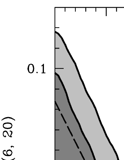
Figure 8.— Constraints on optical depth during reionization divided between two wide ranges in redshift, $\tau(6,20)$ and $\tau(20,z_{\rm max})$, for $z_{\rm max}=30$ (left) and 40 (right). The contours are drawn at 68% (dark gray) and 95% (light gray) 2D marginalized posterior probability. Dashed lines in each panel are lines of constant total optical depth: $\tau=0.12$ for the upper line, and $\tau=0.06$ for the lower line.

Comparison of the two panels in Figure 8 reveals that the choice of $z_{\rm max}$ does not have a large effect on constraints on the optical depth above and below $z=20$. This suggests that $\tau(20,z_{\rm max})$ should be interpreted as $\tau(z>20)$. We provide further justification for this interpretation in § 5.2.

The 95% upper limits on the high-redshift optical depth, $\tau(z>20)$, are $0.076$ and $0.078$ for $z_{\rm max}=30$ and 40, respectively, after marginalizing over all other parameters. This is not a particularly strong constraint, since this result is only marginally inconsistent with all of the optical depth from reionization coming from $z>20$, but with future data it should be possible to either reduce the upper limit on high-$z$ optical depth or to detect the presence of a substantial ionized fraction at high redshift (see § 5.2).

Models of reionization can be tested by computing the principal components of proposed ionization histories and comparing with constraints on $\{m_{\mu}\}$ from Monte Carlo chains. The WMAP constraints in Figure 6 are non-Gaussian, in part because the physicality priors on $\{m_{\mu}\}$ intersect the posterior probability contours where the likelihood is large. Because the constraints do not have a simple Gaussian form, it appears that the full parameter chains are necessary for accurate model testing, although the viability of various models can be estimated by comparing their eigenmode amplitudes with marginalized constraints such as those in Figure 6, keeping in mind that models favored by marginalized constraints could be disfavored in the full $N$-D parameter space.

5.2. Cosmic variance-limited data

To forecast how well principal components of the reionization history could be measured by future CMB polarization experiments, we repeat the analysis of § 5.1 using simulated realizations of the full-sky, noiseless $E$-mode angular power spectrum instead of WMAP data. Any real experiment will of course involve sky cuts, noise, foregrounds, and other complications, so the results presented here represent an optimistic limit on what we can learn about the global reionization history from low-$\ell$ $E$-mode polarization. At the end of this section, we estimate how much the constraints might be degraded from this idealized case for an experiment with characteristics similar to those proposed for the Planck satellite.

We generate simulated realizations of $C_{\ell}^{EE}$ drawn from $\chi^{2}$ distributions with cosmic variance determined by the theoretical angular power spectra that we compute using CAMB. For the $j$th sample in a chain, the likelihood including only $E$-mode polarization is

$$-\ln L_{(j)}=\sum_{\ell}\left(\ell+\frac{1}{2}\right)\left(\frac{\hat{C}_{\ell}^{EE}}{C_{\ell(j)}^{EE}}+\ln\frac{C_{\ell(j)}^{EE}}{\hat{C}_{\ell}^{EE}}-1\right),$$ (16)

where $\hat{C}_{\ell}^{EE}$ is the spectrum of the simulated data and $C_{\ell(j)}^{EE}$ is the theoretical spectrum calculated with the parameter values at step $j$ in the chain.

We have run Monte Carlo chains for multiple realizations of $C_{\ell}^{EE}$ drawn from spectra computed assuming a variety of “true” reionization histories, $x_{e}^{\rm true}(z)$. We start by taking the true history to be a model with nearly instantaneous reionization and $\tau=0.105$. As a contrasting model for comparison we also use an extended, double reionization model with $\tau=0.090$. Figure 1 shows $C_{\ell}^{EE}$ and $x_{e}(z)$ for each of these models.

Since parameter constraints derived using a single draw of $C_{\ell}^{EE}$ from the underlying power spectrum may contain features unique to that realization, we generated Monte Carlo chains for 10 random realizations of the instantaneous reionization power spectrum. Two of these realizations are plotted as points in Figure 9, along with the theoretical spectrum with cosmic variance bands. The thick curves in Figure 9 are spectra of the best-fit models from the Monte Carlo chains for each realization. The overall best-fit models are similar for the two realizations and both agree closely with the theoretical $C_{\ell}^{EE}$. The dashed curve in the right panel of Figure 9 shows an “alternative” best-fit model that we discuss later.

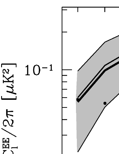
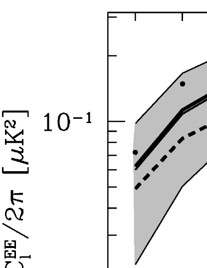
Figure 9.— $E$-mode spectra of the best-fit models from two Monte Carlo chains (thick curves), each using a different realization of simulated cosmic variance-limited data (points). The realizations are drawn from the same $C_{\ell}^{EE}$ of the instantaneous reionization model in Figure 1, plotted as thin curves with shaded regions showing the $1~{}\sigma$ cosmic variance limits. The dashed curve in the right panel shows the best fit model within the high-$m_{2}$ peak in the posterior probability (see Fig. 10).

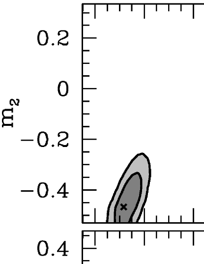
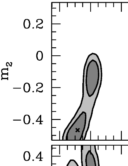
Figure 10.— Marginalized 2D contours (68 and 95%) for the first three principal components with two different realizations of cosmic variance-limited data simulated using the instantaneous reionization history. The fiducial model has maximum redshift $z_{\rm max}=20$, and only the three modes shown here are varied in the parameter chains. The cross in each panel marks the location of the principal components of $x_{e}^{\rm true}(z)$.

The 2D marginalized MCMC constraints on principal components for these two realizations are shown in Figure 10. The plotted regions are bounded by the physical top-hat priors on $\{m_{\mu}\}$ as in Figure 6, but the eigenmodes are different here with $z_{\rm max}=20$ instead of 30 or 40 for the fiducial history. Since we have constructed $x_{e}^{\rm true}(z)$ to have no ionization at $z\gtrsim 15$, we know that $z_{\rm max}=20$ should be a large enough maximum redshift; this choice of $z_{\rm max}$ also reflects the fact that improved empirical determination of $z_{\rm max}$ will allow it to be set at lower redshift for future data analysis, assuming that high-$z$ reionization is not detected.

The contours in Figure 10 show that cosmic variance-limited data can constrain models within the physically allowed parameter space much better than current data can. The chains used for the results shown here vary the first 3 eigenmodes; by running chains with $N>3$ we find that cosmic variance-limited data can provide $2~{}\sigma$ constraints that are tighter than the physicality bounds for the first 4 eigenmodes of a $z_{\rm max}=20$ fiducial model and for at least 5 eigenmodes when $z_{\rm max}=30$.

Although the only difference in the MCMC setup for the left and right panels of Figure 10 is the realization of $C_{\ell}^{EE}$ (Fig. 9), there are some significant differences in the resulting eigenmode constraints, particularly in the $m_{2}-m_{3}$ plane. This kind of variation is typical among the realizations of simulated data, and is related to whether features in the theoretical $C_{\ell}^{EE}$ remain intact with the inclusion of cosmic variance. The relevant features in the spectrum are the small oscillations in the low-power “valley” in $C_{\ell}^{EE}$ on scales $10\lesssim\ell\lesssim 30$. In the example shown here, the feature that matters most is the bump in the theoretical spectrum at $\ell\approx 13$. In the left panel of Figure 9, the $C_{\ell}^{EE}$ realization retains this bump, while in the right panel the bump is washed out by cosmic variance. The result is that the left realization is better able to pick out those reionization models in Monte Carlo chains that reproduce the true $C_{\ell}^{EE}$, leading to the tight constraints on the left side of Figure 10. The realization in the right panel of Figure 9 lacks this important “fingerprint” for identifying models that match the theoretical $C_{\ell}^{EE}$, so the data allow a wider variety of models as reflected in the constraints on the right side of Figure 10. In this case, there are two best-fit models corresponding to the two $68\%$ contours separated in the $m_{2}$ direction. The spectrum of the overall best-fit model (with smaller $m_{2}$), which is close to the theoretical spectrum, is plotted as a thick solid curve in the right panel of Figure 9, while the other best-fit model (at larger $m_{2}$) is plotted as a dashed curve. These two models have significantly different spectra, but because of the scatter in the random draw of $C_{\ell}^{EE}$ they are each able to fit the data better at some multipoles and worse at others in such a way that the high-$m_{2}$ best-fit model is only a slightly worse fit than the low-$m_{2}$ best-fit model.

Among the realizations of simulated data that we explored with MCMC methods, constraints like those in the right panel of Figure 10 are a fairly extreme case, occurring about 10-20% of the time. In general the realizations form a sort of continuum between the two presented here, with about half showing some displacement of the $95\%$ contour towards larger $m_{2}$ but not as much as in the second realization that we show as an example.

The extent to which differences between realizations show up in principal component constraints depends on $x_{e}^{\rm true}(z)$. For example, the $C_{\ell}^{EE}$ for the double reionization model (Fig. 1) have more pronounced oscillations at $\ell\sim 10$-$30$ than the instantaneous reionization spectrum, so they are not as easily erased by cosmic variance or noise and the resulting principal component constraints tend to be more consistent from one realization to the next and more like the left panel of Figure 10.

The differences between constraints from various realizations of simulated data suggest the interesting possibility that our ability to learn about the reionization history from large scale $E$-mode polarization may ultimately depend on the luck of the draw of $C_{\ell}^{EE}$ at our particular vantage point. In an unlucky draw, cosmic variance can distort subtle features in the power spectrum in a way that would limit constraints on reionization eigenmodes to be worse than we might expect from the Fisher approximation or a more typical draw. The good news is that even a realization like the one in the right panels of Figures 9 and 10 would permit constraints that are far better than what is currently possible. It is also important to note that although such constraints are weaker than in the best-case scenario, they are still consistent with the true parameter values and in general would not lead us to rule out the true reionization history based on a principal component analysis of the data.

As with the principal components of $x_{e}(z)$, MCMC analysis indicates that constraints on the total optical depth to reionization would be greatly improved with cosmic variance-limited data: $\sigma_{\tau}\approx 0.005$, down a factor of six from the 3-year WMAP value, $\sigma_{\tau}\approx 0.03$. The constraints on $\tau$ using the realization of instantaneous reionization $C_{\ell}^{EE}$ in the left panel of Figure 9 are listed in Table 1 for two fiducial models with $z_{\rm max}=20$ and 30. Optical depth constraints from the other draw of $C_{\ell}^{EE}$ are similar, so estimates of $\tau$ and $\sigma_{\tau}$ appear not to be biased for atypical realizations. It makes sense that differences in realizations do not significantly affect $\tau$ since the optical depth constraint comes mainly from the peak in $C_{\ell}^{EE}$ on the largest scales whereas differences in principal component constraints between realizations arise from the low-power part of the spectrum at higher $\ell$.

The model-independent constraints on $\tau$ are neither biased nor significantly weaker relative to the constraint obtained assuming instantaneous reionization (bottom row in Table 1), as is true for the WMAP data. This should not be surprising since we have assumed that $x_{e}^{\rm true}(z)$ is an instantaneous reionization model. However, if $x_{e}^{\rm true}(z)$ is in fact very different from the instantaneous model, the estimate of $\tau$ obtained under the assumption of instantaneous reionization will be incorrect. For example, if we take $x_{e}^{\rm true}(z)$ to be the double reionization model of Figure 1, the model-independent approach yields an optical depth constraint consistent with the true value of $\tau=0.090$. On the other hand, MCMC analysis restricted to instantaneous reionization histories gives a significantly biased estimate, $\tau=0.135\pm 0.005$. In this case, the 1D curve of instantaneous reionization models in the space of eigenmodes never lies near the principal component values favored by the data, so any analysis that only considers such models would never find a good fit to the data. This illustrates the importance of a model-independent approach: although results from current data may not be significantly affected by the assumption of a specific form of $x_{e}(z)$, future data will be sensitive enough to the reionization history that the choice of a specific model can greatly impact the results (Holder et al., 2003; Colombo et al., 2005).

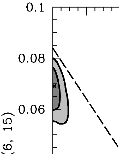
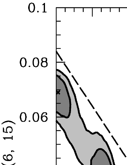
Figure 11.— Same as Figure 8 for simulated cosmic variance-limited data using the two realizations of instantaneous reionization $C_{\ell}^{EE}$ shown in Figure 9. Crosses indicate the partial optical depths for the true reionization history. The redshifts chosen for $z_{\rm mid}$ and $z_{\rm max}$ are also lower here than for the WMAP analysis, reflecting the expectation that future data may permit better empirical constraints on $z_{\rm max}$.

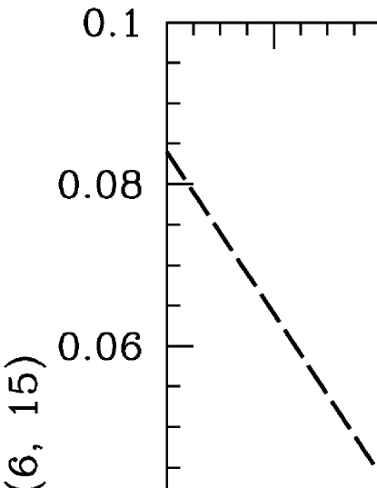
Figure 12.— Same as Figure 11, but assuming that $x_{e}^{\rm true}(z)$ is a double reionization history with $z_{\rm max}=23$ (thin curves in Figure 1). Crosses mark the true partial optical depths for this model; note that unlike in Figure 11, $\tau(15,20)\neq\tau(15,30)$ for the expected values here since $x_{e}^{\rm true}(z)$ has a nonzero ionized fraction between redshifts 20 and 30.

Though constraints on the contributions to $\tau$ from high and low $z$ are currently limited to weak upper bounds, future polarization data will likely enable more definitive detections of high-$z$ reionization if it is present, or tighter upper limits if absent. The left and right panels of Figure 11 show these constraints from Monte Carlo chains using the $C_{\ell}^{EE}$ plotted in the left and right panels of Figure 9, respectively. The true ionization history has zero ionized fraction at $z>15$, and the MCMC analysis places a 95% CL upper limit on $\tau(z>15)$ of $\sim 0.03$. Figure 12 shows MCMC constraints on the same partial optical depths using simulated data where the true model is instead taken to be the extended, double reionization history plotted as a thin curve in the inset of Figure 1. In this case, most of $\tau(z_{\rm min},z_{\rm max})$ comes from $z>15$, and using the principal components of $x_{e}(z)$ the high-$z$ optical depth can be detected at a high level of confidence and measured to an accuracy of $\sim 0.01$. Note that the constraints in both Figures 11 and 12 are consistent with the WMAP constraints in Figure 8.

As with WMAP data, most of the constraints from simulated data in Figures 11 and 12 do not appear to depend strongly on the choice of $z_{\rm max}$. For the instantaneous reionization model used for Figure 11, this is to be expected since we know that the simulated $C_{\ell}^{EE}$ have no contribution from $z\gtrsim 20$. Each set of contours in Figure 11 is consistent with the values of $\tau(6,15)$ and $\tau(15,z_{\rm max})$ for $x_{e}^{\rm true}(z)$. The constraints in the second panel in Figure 11 extend to larger high-$z$ optical depth than those in the first panel because the effect of the physicality priors is not as strong at larger $z_{\rm max}$, as noted in § 5.1; the leftmost $z_{\rm max}=20$ contours would stretch to larger $\tau(15,20)$ and smaller $\tau(6,15)$ if we did not apply the physicality bounds. The two panels on the right side of Figure 11 show weaker constraints on the partial optical depths because the principal component constraints for that realization of $C_{\ell}^{EE}$ are weaker.

In the extended, double reionization model used for Figure 12, reionization actually starts at $z=23$, so the choice of $z_{\rm max}=20$ is not appropriate for this model. The result of such an error is that the constraint on $\tau(15,20)$ is inconsistent with the true value, marked by a cross in the left panel of Figure 12. The $z_{\rm max}=30$ constraints in the right panel are consistent with the expected value, although not in perfect agreement due to cosmic variance. It is interesting that although the value chosen for $z_{\rm max}$ in the left panel is too low for this model, the constraints on $\tau(z>15)$ for $z_{\rm max}=20$ and $z_{\rm max}=30$ are still consistent with each other. This supports the interpretation of constraints on $\tau(z_{\rm mid},z_{\rm max})$ as $\tau(z>z_{\rm mid})$ in § 5.1

While the cosmic variance-limited simulated data are useful for determining how well the reionization history could possibly be constrained by large-scale $E$-mode polarization measurements, it is also interesting to ask how well we can do with future experiments that fall somewhat short of the idealized case that we have considered so far. In particular, the upcoming Planck satellite is expected to improve our knowledge of the large-scale $E$-mode spectrum substantially (The Planck Collaboration, 2006); what does this imply for constraints on $x_{e}(z)$? To estimate what might be possible with Planck data, we assume that after subtracting foregrounds a single foreground-free frequency channel remains for constraining the low-$\ell$ $E$-mode polarization. We take this to be the 143 GHz channel with a white noise power level of $w_{P}^{-1/2}=81~{}\mu$K^′ and beam size $\theta_{\rm FWHM}=7.1^{\prime}$, and we assume that the sky coverage is $f_{\rm sky}=0.8$ after cutting out the Galactic plane (The Planck Collaboration, 2006; Albrecht et al., 2006). We compute the likelihood of Monte Carlo samples using the routines provided in CosmoMC and analyze parameter chains with the principal component method as described for WMAP and cosmic variance-limited data.

For various choices of $x_{e}^{\rm fid}(z)$ and $x_{e}^{\rm true}(z)$ we find that going from full-sky cosmic variance-limited data to Planck-like data increases the uncertainty in $x_{e}(z)$ principal components, $\sigma_{\mu}$, and in the optical depth, $\sigma_{\tau}$, by roughly a factor of two. Based on these results, it should be possible to constrain about three eigenmodes at $\sim 2~{}\sigma$ within the space of physical models, and we expect $\tau$ to be determined to an accuracy of about $\pm 0.01$. This is consistent with previous estimates of the Planck optical depth uncertainty when considering more general reionization models than instantaneous reionization (e.g., Holder et al., 2003; Hu & Holder, 2003).

5.3. Fisher matrix predictions versus MCMC results

The Fisher matrix analysis of § 2 predicts that the principal components of $x_{e}(z)$ should be uncorrelated, with errors given by $\sigma_{\mu}$ from equation (2) (in the idealized limit of full sky, noiseless observations). These characteristics rely on the assumption that the difference between the true and fiducial reionization histories is small: $\delta x_{e}^{\rm true}(z)=x_{e}^{\rm true}(z)-x_{e}^{\rm fid}(z)\ll 1$. Clearly this assumption will not hold for any single fiducial history if one wants to consider a variety of possible true histories, and the consequence is that $\langle m_{\mu}m_{\nu}\rangle$ differs from $\sigma_{\mu}^{2}\delta_{\mu\nu}$.

Figure 13.— Monte Carlo constraints in the $m_{1}$-$m_{2}$ plane from the left panel of Figure 10 (68 and 95% contours) compared with the estimated constraints from the Fisher matrix (shaded contours).

As an example of the difference between the Fisher approximation and the full Monte Carlo analysis, in Figure 13 the marginalized constraints in the $m_{1}-m_{2}$ plane from the left panel of Figure 10 are compared with the Fisher matrix error ellipses, centered on the true $(m_{1},m_{2})$ for the same choices of $x_{e}^{\rm true}(z)$ (instantaneous reionization with $\tau=0.105$) and $x_{e}^{\rm fid}(z)$ (constant $x_{e}=0.15$ out to $z_{\rm max}=20$). The MCMC constraints have correlated values of $m_{1}$ and $m_{2}$ with somewhat larger uncertainties than the Fisher matrix $\{\sigma_{\mu}\}$. The eigenfunctions, $S_{\mu}(z)$, are constructed to have orthogonal effects on $C_{\ell}^{EE}$ in the vicinity of the fiducial model, but for large $\delta x_{e}(z)$ the orthogonality breaks down. Fortunately the errors on $\tau$ remain largely unaffected because the $m_{1}-m_{2}$ correlation is oriented such that the increased errors are along the direction of constant total $\tau$ (see Figure 7).

One can compute new eigenfunctions by evaluating $\partial \ln C_{\mathrm{\ell }}^{EE}/\partial x_e(z$

References

- Albrecht et al. (2006) Albrecht, A., Bernstein, G., Cahn, R., Freedman, W. L., Hewitt, J., Hu, W., Huth, J., Kamionkowski, M., Kolb, E. W., Knox, L., Mather, J. C., Staggs, S., & Suntzeff, N. B. 2006, ArXiv Astrophysics e-prints astro-ph/0609591
- Barkana & Loeb (2001) Barkana, R. & Loeb, A. 2001, Phys. Rep., 349, 125
- Brooks & Gelman (1998) Brooks, S. P. & Gelman, A. 1998, Journal of Computational and Graphical Statistics, 7, 434
- Christensen et al. (2001) Christensen, N., Meyer, R., Knox, L., & Luey, B. 2001, Class. Quant. Grav., 18, 2677
- Colombo et al. (2005) Colombo, L. P. L., Bernardi, G., Casarini, L., Mainini, R., Bonometto, S. A., Carretti, E., & Fabbri, R. 2005, A&A, 435, 413
- Doré et al. (2007) Doré, O., Holder, G., Alvarez, M., Iliev, I. T., Mellema, G., Pen, U.-L., & Shapiro, P. R. 2007, ArXiv Astrophysics e-prints astro-ph/0701784
- Dunkley et al. (2005) Dunkley, J., Bucher, M., Ferreira, P. G., Moodley, K., & Skordis, C. 2005, Mon. Not. Roy. Astron. Soc., 356, 925
- Fan et al. (2006) Fan, X.-H., Carilli, C. L., & Keating, B. 2006, Ann. Rev. Astron. Astrophys., 44, 415
- Gelman & Rubin (1992) Gelman, A. & Rubin, D. B. 1992, Statistical Science, 7, 457
- Holder et al. (2003) Holder, G. P., Haiman, Z., Kaplinghat, M., & Knox, L. 2003, ApJ, 595, 13
- Hu (2000) Hu, W. 2000, ApJ, 529, 12
- Hu & Holder (2003) Hu, W. & Holder, G. P. 2003, Phys. Rev. D, 68, 023001
- Hu & White (1997) Hu, W. & White, M. 1997, ApJ, 479, 568
- Iliev et al. (2006) Iliev, I. T., Pen, U.-L., Richard Bond, J., Mellema, G., & Shapiro, P. R. 2006, New Astronomy Review, 50, 909
- Kaplinghat et al. (2003) Kaplinghat, M., Chu, M., Haiman, Z., Holder, G. P., Knox, L., & Skordis, C. 2003, ApJ, 583, 24
- Kasuya et al. (2004) Kasuya, S., Kawasaki, M., & Sugiyama, N. 2004, Phys. Rev. D, 69, 023512
- Kosowsky et al. (2002) Kosowsky, A., Milosavljevic, M., & Jimenez, R. 2002, Phys. Rev., D66, 063007
- Lewis & Bridle (2002) Lewis, A. & Bridle, S. 2002, Phys. Rev. D, 66, 103511
- Lewis et al. (2000) Lewis, A., Challinor, A., & Lasenby, A. 2000, ApJ, 538, 473
- Lewis et al. (2006) Lewis, A., Weller, J., & Battye, R. 2006, MNRAS, 373, 561
- Mortonson & Hu (2007) Mortonson, M. J. & Hu, W. 2007, ApJ, 657, 1
- Naselsky & Chiang (2004) Naselsky, P. & Chiang, L.-Y. 2004, MNRAS, 347, 795
- Page et al. (2006) Page, L., Hinshaw, G., Komatsu, E., Nolta, M. R., Spergel, D. N., Bennett, C. L., Barnes, C., Bean, R., Doré, O., Halpern, M., Hill, R. S., Jarosik, N., Kogut, A., Limon, M., Meyer, S. S., Odegard, N., Peiris, H. V., Tucker, G. S., Verde, L., Weiland, J. L., Wollack, E., & Wright, E. L. 2006, ArXiv Astrophysics e-prints astro-ph/0603450
- Raftery & Lewis (1992) Raftery, A. E. & Lewis, S. M. 1992, in Bayesian Statistics, ed. J. M. Bernado (OUP), 765
- Spergel et al. (2006) Spergel, D. N., Bean, R., Doré, O., Nolta, M. R., Bennett, C. L., Hinshaw, G., Jarosik, N., Komatsu, E., Page, L., Peiris, H. V., Verde, L., Barnes, C., Halpern, M., Hill, R. S., Kogut, A., Limon, M., Meyer, S. S., Odegard, N., Tucker, G. S., Weiland, J. L., Wollack, E., & Wright, E. L. 2006, ArXiv Astrophysics e-prints astro-ph/0603449
- The Planck Collaboration (2006) The Planck Collaboration. 2006, ArXiv Astrophysics e-prints astro-ph/0604069
- Zaldarriaga (1997) Zaldarriaga, M. 1997, Phys. Rev. D, 55, 1822