One- and two-component bottle-brush polymers: simulations
compared to theoretical predictions
Summary: Scaling predictions and results from self-consistent field calculations for bottle-brush polymers with a rigid backbone and flexible side chains under good solvent conditions are summarized and their validity and applicability is assessed by a comparison with Monte Carlo simulations of a simple lattice model. It is shown that under typical conditions, as they are also present in experiments, only a rather weak stretching of the side chains is realized, and then the scaling predictions based on the extension of the Daoud-Cotton blob picture are not applicable.
Also two-component bottle brush polymers are considered, where two types (A,B) of side chains are grafted, assuming that monomers of different kind repel each other. In this case, variable solvent quality is allowed for, such that for poor solvent conditions rather dense cylinder-like structures result. Theories predict “Janus Cylinder”-type phase separation along the backbone in this case. The Monte Carlo simulations, using the pruned-enriched Rosenbluth method (PERM) then are restricted to rather short side chain length. Nevertheless, evidence is obtained that the phase separation between an A-rich part of the cylindrical molecule and a B-rich part can only occur locally. The correlation length of this microphase separation can be controlled by the solvent quality. This lack of a phase transition is interpreted by an analogy with models for ferromagnets in one space dimension.
I. Introduction
Flexible macromolecules can be grafted to various substrates by special endgroups. Such “polymer brushes” find widespread applications and also pose challenging theoretical problems, such as an understanding of the conformational statistics and resulting geometrical structure of these tethered chain molecules. Only this latter aspect shall be considered in the present paper, for chains grafted to a straight line or a very narrow cylinder. This problem is a limiting case of “bottle brush” polymers where side chains are grafted to a long macromolecule that forms the backbone of the bottle brush. When this backbone chain is also a flexible polymer and the grafting density is not very high, a “comb polymer” results, which is outside of consideration here. Also we shall not discuss the case where the backbone chain is very short, so the conformation would resemble a “star polymer”. Here we restrict attention to either stiff backbone chains or high grafting density of side chains at flexible backbones. In the lattice case stiffening of the backbone occurs due to excluded volume interactions, and a cylindrical shape of the molecule as a whole results. In fact, many experiments have been carried out where with an appropriate chemical synthesis bottle brush polymers with a worm-like cylindrical shape were produced . The recent papers contain a more detailed bibliography on this rapidly expanding field.
On the theoretical side, two aspects of the conformation of bottle brush polymers where mostly discussed: (i) conformation of a side chain when the backbone can be treated as a rigid straight line or thin cylinder (ii) conformation of the whole bottle brush when the backbone is (semi)flexible. The latter problem is left out of consideration in the present paper. Problem (i), the stretching of the side chains in the radial direction in the case of sufficiently high grafting density, was mostly discussed in terms of a scaling description, extending the Daoud-Cotton “blob picture” from star polymers to bottle brush polymers. If one uses the Flory exponent in the scaling relation for the average root mean square end-to-end distance of a side chain, , where is the grafting density and N is the number of effective monomeric units of a side chain, one obtains . These exponents happen to be identical to those which one would obtain assuming that the chains attain quasi-two-dimensional configurations, resulting if each chain is confined to a disk of width . Although this latter picture is a misconception, in experimental studies (e.g. 14 ; 15 ) this hypothesis of quasi-two-dimensional chains is discussed as a serious possibility. Therefore we find it clearly necessary to first review the correct scaling theory based on the blob picture, and discuss in detail what quantities need to be recorded in order to distinguish between these concepts. Thus, in the next section we shall give a detailed discussion of the scaling concepts for bottle brush polymers with rigid backbones.
Thereafter we shall describe the Monte Carlo test of these predictions, that we have recently performed using the pruned enriched Rosenbluth method (PERM). After a brief description of the Monte Carlo methodology, we present our numerical results and compare them to the pertinent theoretical predictions.
In the second part of this paper, we discuss the extension from one-component to two-component bottle brush polymers. Just as in a binary polymer blend (A,B) typically the energetically unfavorable interaction (described by the Flory-Huggins parameter ) should cause phase separation between A-rich and B-rich domains. However, just as in block copolymers where A chains and B-chains are tethered together in a point, no macroscopic phase separation but only “microphase separation” is possible: for a binary (A,B) bottle brush with a rigid backbone one may expect formation of “Janus Cylinder” structures. This means, phase separation occurs such that the A-chains assemble in one half of the cylinder, the B chains in the other half, separated from the A-chains via a flat interface containing the cylinder axis. However, it has been argued that the long range order implied by such a “Janus cylinder” type structure has a one-dimensional character, and therefore true long range order is destroyed by fluctuations at nonzero temperature. Only local phase separation over a finite correlation length along the cylinder axis may persist.
We shall again first review the theoretical background on this problem, and then describe the simulation evidence. We conclude our paper by a summary and outlook on questions that are still open, briefly discussing also possible consequences on experimental work. However, we shall not deal with the related problems of microphase separation of a bottle brush with only one kind of side chains induced by deterioration of the solvent quality or by adsorption on flat substrates.
II. Conformation of Side Chains of Bottle Brushes under Good Solvent Conditions: Theoretical Background
The most straightforward approach to understand the conformations of chains in polymer brushes and star polymers under good solvent conditions uses the concept to partition the space available for the chains into compartments, called “blobs”. The idea is that in each such region there occur only monomers of one chain, no monomers of any other chains occur in such a blob, and hence self-avoiding walk statistics holds in each blob. This means, if a (spherical) blob has a radius and contains monomers, these numbers must be related via
| (1) |
Here is a length of the order of the size of an effective monomer, and we emphasize from the start that it is crucial to use the correct value of the self-avoiding walk exponent , as it is provided from renormalization group calculations or accurate Monte Carlo simulations. If one would ignore the small difference between and the Flory estimate 3/5, one would already miss an important distinction between two different scaling regimes for a brush on a flat substrate. An almost trivial condition of this “blobology” is that each of the effective monomeric units of a chain must belong to some blob. So we have
| (2) |
where is the number of blobs belonging to one particular chain.
Finally we note that the space available to the chains must be densely filled with blobs. It then remains to discuss which factors control the blob size . The simplest case is a polymer brush on a flat substrate (under good solvent conditions, as assumed here throughout): if we neglect, for simplicity, any local fluctuations in the grafting density, the distance between grafting sites simply is given by . Putting in Equation (1), we find , i.e. each chain is a string of blobs. According to the simple-minded description of polymer brushes due to Alexander, this string simply is arranged like a one-dimensional cigar, and one would conclude that the height of a flat brush is
| (3) |
The free end of the chain is in the last blob and hence the end-to-end distance in this “Alexander picture” of polymer brushes. However, a more detailed theory of polymer brushes, such as the self-consistent field theory in the strong stretching limit, yields a somewhat different behavior: the end monomer is not localized at the outer edge of the brush, but rather can be located anywhere in the brush, according to a broad distribution; also the monomer density in polymer brushes at flat substrates is not constant up to the brush height , but rather decreases according to a parabolic profile. So even for a polymer brush at a flat substrate already a description in terms of non-uniform blob sizes, that increase with increasing distance from the substrate, is required. However, in the following we shall disregard all these caveats about the Alexander picture for flat brushes, and consider its generalization to the bottle brush geometry, where polymer chains are tethered to a line rather than a flat surface. Then we have to partition space into blobs of nonuniform size and shape in order to respect the cylindrical geometry (Figure 1).
In the discussion of brushes in cylindrical geometry in terms of blobs in the literature the non-spherical character of the blob shape is not explicitly accounted for, and it rather is argued that one can characterize the blobs by one effective radius depending on the radial distance from the cylinder axis. One considers a segment of the array of length containing polymer chains. On a surface of a cylinder of radius and length there should then be blobs, each of cross-sectional area ; geometrical factors of order unity are ignored throughout. Since the surface area of the cylindrical segment is , we must have
| (4) |
If the actual non-spherical shape of the blobs (Figure 1) is neglected, the blob volume clearly is of the order of . Invoking again the principle that inside a blob self-avoiding walk statistics hold, we have, in analogy with Equation (1),
| (5) |
From this result one immediately derives the power law decay for the density profile as follows
| (6) | |||||
Using the Flory approximation one would find instead.
Now the average height of the bottle brush is estimated by requiring that we obtain all monomers per unit length in the z-direction along the axis of the bottle brush (cf. Figure 1) when we integrate from to ,
| (7) |
This yields, again ignoring factors of order unity,
| (8a) | |||
| (8b) |
Note that the use of the Flory estimate would simply yield , which happens to be identical to the relation that one obtains when one partitions the cylinder of height and radius into disks of height , requiring hence that each chain is confined strictly into one such disk. Then each chain would form a quasi-two-dimensional self-avoiding walk formed from blobs of diameter . Since we have again, we would conclude that the end-to-end distance of such a quasi-two-dimensional chain is
| (9) | |||||
Putting then , Equation (8b) results when we use there . However, this similarity between Equations (8b), (9) is a coincidence: in fact, the assumption of a quasi-two-dimensional conformation does not imply a stretching of the chain in radial direction. In fact, when we put the x-axis of our coordinate system in the direction of the end-to-end vector of the chain, we would predict that the y-component of the gyration radius scales as
| (10) |
since for quasi-two-dimensional chains we have , all these linear dimensions scale with the same power laws. On the other hand, if the Daoud-Cotton-like picture {Figure 1a} holds, in a strict sense, one would conclude that is of the same order as the size of the last blob for ,
| (11) | |||||
Clearly this prediction is very different from Equation (10), even with the Flory exponent we find from Equation (11) that . Hence it is clear that an analysis of all three components of the gyration radius of a polymer chain in a bottle brush is very suitable to distinguish between the different versions of scaling concepts discussed in the literature.
However, at this point we return to the geometrical construction of the filling of a cylinder with blobs, Figure 1. We explore the consequences of the obvious fact that the blobs cannot be simple spheres, when we require that each blob contains monomers from a single chain only, and the available volume is densely packed with blobs touching each other.
As mentioned above, was defined from the available surface area of a cylinder at radius , cf. Equation (4). It was argued that for each chain in the surface area of such a cylinder a surface area is available. However, consideration of Figure 1 shows that these surfaces are not circles but rather ellipses, with axes and . The blobs hence are not spheres but rather ellipsoids, with three different axes: in z-direction along the cylinder axes, in the y-direction tangential on the cylinder surface, normal to both the z-direction and the radial direction, and the geometric mean of these two lengths , in the radial x-direction. Since the physical meaning of a blob is that of a volume region in which the excluded volume interaction is not screened, this result implies that the screening of excluded volume in a bottle brush happens in a very anisotropic way: there are three different screening lengths, in the axial z-direction, in the radial x-direction, and in the third, tangential, y-direction. Of course, it remains to be shown by a more microscopic theory that such an anisotropic screening actually occurs.
However, the volume of the ellipsoid with these three axes still is given by the formula
| (12) |
with given by Equation (4), and hence the volume of the blob has been correctly estimated by the spherical approximation. As a consequence, the estimations of the density profile , Equation (6), and resulting brush height , Equation (8b), remain unchanged.
More care is required when we now estimate the linear dimensions of the chain in the bottle brush. We now orient the x-axis such that the xz-plane contains the center of mass of the considered chain. As Figure 1b indicates, we can estimate assuming a random walk picture in terms of blobs. When we go along the chain from the grafting site towards the outer boundary of the bottle brush, the blobs can make excursions with , independent of . Hence we conclude, assuming that the excursions of the steps add up randomly
| (13) |
Hence we must estimate the number of blobs per chain in a bottle brush. We must have
| (14) |
Note from Figure 1 that we add an increment to when we go from the shell to shell in the cylindrical bottle brush. So the discretization of the integral in Equation (14) is equivalent to the sum. From Equation (14) we then find, again ignoring factors of order unity
| (15) |
and consequently
| (16) |
With Flory exponents we hence conclude , and thus . The estimation of is most delicate, of course, because when we consider random excursions away from the radial directions, the excursions are non-uniform. So we have instead of Equation (One- and two-component bottle-brush polymers: simulations compared to theoretical predictions),
| (17) |
in analogy with Equation (14). This yields and hence
| (18) | |||||
while the corresponding result with Flory exponents is . These different results for {Equation (8b)}, {Equation (18)} and {Equation (16)} clearly reflect the anisotropic structure of a chain in a bottle brush. Note that the result for according to Equation (18) is much larger than the simple Daoud-Cotton-like prediction, Equation (11), but is clearly smaller than the result of the quasi-two-dimensional picture, Equation (10).
As a consistency check of our treatment, we note that also Equation (7) can be formulated as a discrete sum over blobs
| (19) |
which yields Equation (8a), as it should be.
Finally we discuss the crossover towards mushroom behavior. Physically, this must occur when the distance between grafting points along the axis, , becomes equal to . Thus we can write
| (20) |
where we have absorbed the extra factor in the scaling function . We note that Equation (8b) results from Equation (20) when we request that
| (21) |
and hence a smooth crossover between mushroom behavior and radially stretched polymer conformations occurs for of order unity, as it should be. Analogous crossover relations can be written for the other linear dimensions, too:
| (22) |
| (23) |
The agreement between Equation (16) and Equation (22) or Equation (18) and Equation (23), respectively, provides a check on the self-consistency of our scaling arguments.
However, it is important to bear in mind that the blob picture of polymer brushes, as developed by Alexander, Daoud and Cotton, Halperin and many others, is a severe simplification of reality, since its basic assumptions that (i) all chains in a polymer brush are stretched in the same way, and (ii) the chain ends are all at a distance from the grafting sites, are not true. Treatments based on the self-consistent field theory and computer simulations have shown that chain ends are not confined at the outer boundary of the brush, and the monomer density distribution is a nontrivial function, that cannot be described by the blob model. However, it is widely believed that the blob model yields correctly the power laws of chain linear dimensions in terms of grafting density and chain length, so the shortcomings mentioned above affect the pre-factors in these power laws only. In this spirit, we have extended the blob model for brushes in cylindrical geometry in the present section, taking the anisotropy in the shape of the blobs into account to predict the scaling behavior of both the brush height (which corresponds to the chain end-to-end distance and the x-component of the gyration radius) and of the transverse gyration radius components . To our knowledge, the latter have not been considered in the previous literature.
III. Monte Carlo Methodology
We consider here the simplest lattice model of polymers under good solvent conditions, namely, the self-avoiding walk on the simple cubic lattice. The backbone of the bottle brush is just taken to be the z-axis of the lattice, and in order to avoid any effects due to the ends of the backbone, we choose periodic boundary conditions in the z-direction. The length of the backbone is taken to be lattice spacings, and the lattice spacing henceforth is taken as one unit of length. Note that in order to avoid finite size effects has to be chosen large enough so that no side chain can interact with its own “images” created by the periodic boundary condition, i.e. .
We create configurations of the bottle brush polymers applying the pruned-enriched-Rosenbluth method (PERM). This algorithm is based on the biased chain growth algorithm of Rosenbluth and Rosenbluth, and extends it by re-sampling technique (“population control”) with depth-first implementation. Similar to a recent study of star polymers all side chains of the bottle brush are grown simultaneously, adding one monomer to each side chain one after the other before the growth process of the first chain continues by the next step.
When a monomer is added to a chain of length (containing monomers) at the th step, one scans the neighborhood of the chain end to identify the free neighboring sites of the chain end, to which a monomer could be added. Out of these sites available for the addition of a monomer one site is chosen with the probability for the th direction. One has the freedom to sample these steps from a wide range of possible distributions, e.g. , if one site is chosen at random, and this additional bias is taken into account by suitable weight factors. The total weight of a chain of length with an unbiased sampling is determined recursively by . While the weight is gained at the th step with a probability , one has to use instead of . The partition sum of a chain of length (at the th step) is approximated as
| (24) |
where is the total number of configurations , and averages of any chain property (e.g. its end-to-end distance, gyration radius components, etc.) are obtained as
| (25) |
As is well-known from Ref. 84 , for this original biased sampling the statistical errors for large are very hard to control. This problem is alleviated by population control. One introduces two thresholds
| (26) |
where is the current estimate of the partition sum, and and are constants of order unity. The optimal ratio between and is found to be in general. If exceeds for the configuration , one produces identical copies of this configuration, replaces their weight by , and uses these copies as members of the population for the next step, where one adds a monomer to go from chain length to . However, if , one draws a random number , uniformly distributed between zero and one. If , the configuration is eliminated from the population when one grows the chains from length to . This “pruning” or “enriching” step has given the PERM algorithm its name. On the other hand, if , one keeps the configuration and replaces its weight by . In a depth-first implementation, at each time one deals with only a single configuration until a chain has been grown either to the end of reaching the maximum length or to be killed in between, and handles the copies by recursion. Since only a single configuration has to be remembered during the run, it requires much less memory.
In our implementation, we used and for the first configuration hitting chain length . For the following configurations, we used and , here is a positive constant, and is the total number of configurations of length already created during the run. The bias of growing side chains was used by giving higher probabilities in the direction where there are more free next neighbor sites and in the outward directions perpendicular to the backbone, where the second part of bias decreases with the length of side chains and increases with the grafting density. Totally independent configurations were obtained in most cases we simulated.
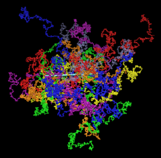
Typical simulations used backbone lengths and 128, (one chain per grafting site of the backbone, although occasionally also and were used), and grafting densities , , , , and . The side chain length was varied up to . So a typical bottle brush with (i.e., side chains) and contains a total number of monomers . Figure 2 shows a snapshot configuration of such a bottle brush polymer. Note that most other simulation algorithms for polymers would fail to produce a large sample of well-equilibrated configurations of bottle brush polymers of this size: dynamic Monte Carlo algorithms using local moves involve a relaxation time (in units of Monte Carlo steps per monomer [MCS]) of order where if one assumes that the side chains relax independently of each other and one applies the Rouse model in the good solvent regime. For such an estimate would imply that the time between subsequent statistically independent configurations is of the order of 107 MCS, which clearly is impractical. While the pivot algorithm would provide a significantly faster relaxation in the mushroom regime, the acceptance rate of the pivot moves quickly deteriorates when the monomer density increases. This algorithm could equilibrate the outer region of the bottle brush rather efficiently, but would fail to equilibrate the chain configurations near the backbone. The configurational bias algorithm would be an interesting alternative when the monomer density is high, but it is not expected to work for very long chains, such as . Also, while the simple enrichment technique is useful to study both star polymers and polymer brushes on flat substrates it also works only for chain lengths up to about . Thus, existing Monte Carlo simulations of one-component bottle brushes under good solvent conditions either used the bond fluctuation model on the simple cubic lattice applying local moves with side chain lengths up to or or the pivot algorithm with side chain lengths up to , but considering flexible backbone of length . An alternative approach was followed by Yethiraj who studied an off-lattice tangent hard sphere model by a pivot algorithm in the continuum, for . All these studies addressed the question of the overall conformation of the bottle brush for a flexible backbone, and did not address in detail the conformations of the side chains. Only the total mean square radius of gyration of the side chains was estimated occasionally, obtaining or and . However, due to the smallness of the side chain lengths used in these studies, as quoted above, these results have to be considered as somewhat preliminary, and also a systematic study of the dependence on both and was not presented. We also note that the conclusions of the quoted papers are somewhat contradictory.
An interesting alternative simulation method to the Monte Carlo study of polymeric systems is Molecular Dynamics, of course. While in corresponding studies of a bead-spring model of polymer chains for flat brushes chain lengths up to were used, for chains grafted to thin cylinders the three chain lengths and 150 were used. For , also four values of grafting density were studied. Murat and Grest used these data to test the scaling prediction for the density profile, Equation (6), but found that is better compatible with rather than . However, for the range where the power law is supposed to apply is very restricted, and hence this discrepancy was not considered to be a problem for the theory.
Thus, we conclude that only due to the use of the PERM algorithm has it become possible to study such large bottle brush polymers as depicted in Figure 2. Nevertheless, as we shall see in the next section, even for such large side chain lengths one cannot yet reach the asymptotic region where the power laws derived in the previous section are strictly valid.
IV. Monte Carlo Results for One-Component Bottle-Brush Polymers
In Figures 3 and 4, we present our data for the mean square end-to-end radii and gyration radii components of the side chains. Note that for each chain configuration a separate local coordinate system for the analysis of the chain configuration needs to be used; while the z-axis is always oriented simply along the backbone, the x-axis is oriented perpendicular to the z-axis and goes through the center of mass of the chain in this particular configuration. The y-axis then also is fixed simply from the requirement that it is perpendicular to both the x- and z-axes.
For a polymer mushroom (which is obtained if the grafting density is sufficiently small) we expect that all chain linear dimensions scale as , for sufficiently long chains. Therefore we have normalized all mean square linear dimensions in Figures 3 and 4 by a factor , using the theoretical value . However, as we see from Figures 3, 4 in the range displayed there, even for the smallest presented, where a single side chain is simulated, the shown ratios are not constant. This fact indicates that corrections to scaling should not be disregarded, and this problem clearly complicates the test of the scaling predictions derived above. For the largest value of included , the irregular behavior of some of the data (Figure 3b,c, Figure 4b) indicate a deterioration of statistical accuracy. This problem gets worse for increasing number of side chains .
A further complication is due to the residual finite size effect. Figure 5 shows a plot of vs. the scaling variable . One can recognize that for small but large and not too large systematic deviations from scaling occur (Figure 5a), which simply arise from the fact that an additional scaling variable (related to ) comes into play when no longer is negligibly smaller than . While for real bottle brush polymers with stiff backbone effects due to the finite lengths of the backbone are physically meaningful and hence of interest, the situation is different in our simulation due to the use of periodic boundary conditions. The choice of periodic boundary conditions is motivated by the desire to study the characteristic structure in a bottle brush polymer far away from the backbone ends, not affected by any finite size effects. However, if becomes comparable to , each chain interacts with its own periodic images, and this is an unphysical, undesirable, finite size effect. Therefore in Figure 5b, the data affected by such finite size effects are not included. One finds a reasonable data collapse of the scaled mean square end-to-end distance when one plots the data versus the scaling variable . These results constitute the first comprehensive test of the scaling relations for bottle brush polymers, Equations (21) - (23), and the consistency between the data and the proposed scaling structure in terms of the variable is indeed very gratifying. On the other hand, it is also evident from Figures 5 and 6 that only a mild stretching of the side chains away from the backbone is observed, and in this region one is still far away from the region of strong stretching, where the simple power laws Equations (8b), (18) and (16) apply. Obviously, the crossover from the simple mushroom behavior (observed for ) to the strongly stretched bottle brush (observed for ) takes at least one decade of the scaling variable . There is a rather gradual and smooth crossover rather than a kink-like behavior of the scaling function. While in the -component at least near a weak onset of stretching can be recognized, hardly any evidence for the contraction of the and -components is seen.
In order to test what one would expect if the picture of the chains as quasi-two-dimensional self-avoiding walks were correct, we have also studied single chains grafted to a straight backbone of length , which are confined between two parallel repulsive infinite walls. The grafting site of the chains was chosen at the site located symmetrically between the confining walls in the slit {if the grafting site is chosen to be the origin of the coordinate system, the confining hard walls occur at }. Figure 7 gives log-log plots of the gyration radii components of such chains confined to such disk-like slits, which we denote as , and , in order to distinguish then from the actual gyration radii components of the side chains in a bottle brush polymer. One can clearly see that , scale as for large , as it must be. These data are very similar to data for chains confined between repulsive walls without a grafting to a piece of a rigid backbone, of course. In the corresponding scaling plot (Figure 8) one can see that both and have the simple crossover scaling behavior
| (27) |
with with , as expected, and seen in related previous work. Obviously, although we use in Figures 7 and 8 the same range of and as in Figures 4 and 6, the behavior is rather different. As expected from our scaling analysis presented above, the confinement that a chain experiences in a bottle brush due to the presence of the other chains is much weaker than the confinement of a chain in the equivalent disk-like sector between confining walls. This fact is demonstrated very directly in Figure 9, where the ratios are plotted vs. for the corresponding values of . If the hypothesis of quasi-two dimensional confinement were valid, we would expect these ratios to be constants. Obviously, this is not the case.
As a final point of this section, we discuss the distribution of monomers (Figures 10 and 11) and chain ends (Figures 12 and 13) in the simulated model for the bottle brush polymer. Unlike corresponding radial density distributions for the off-lattice bead-spring model of Murat and Grest, where for small distances close to the backbone a kind of “layering” was observed, we see a rather smooth behavior also for small distances (Figure 10). For larger distances, the behavior is qualitatively very similar. Again we fail to provide a clear-cut evidence for the predicted power law decay, Equation (6). Note, however, that this power law is supposed to hold only in the strong stretching limit, where Equation (8b) is observable (which we do not verify either), and in addition the stringent condition needs to be obeyed, to have this power law. Although our simulations encompass much longer chains than every previous work on bottle brushes, we clearly fail to satisfy this double inequality.
Turning to the distribution along the backbone (Figure 11), the periodicity due to the strictly periodic spacing of grafting sites is clearly visible. If desired, one could also study a random distribution of grafting sites along the backbone, of course, but we have restricted attention to the simplest case of a regular arrangement of grafting sites only. The distribution of chain ends exhibits an analogous periodicity for small values of only, while is approximately constant (Figure 12) for larger values of .
Most interesting is the radial distribution of chain ends (Figure 13). One can see an increasing depression of for small when increases. Again these data are similar to the off-lattice results of Murat and Grest. In no case do we see the “dead zone” predicted by the self-consistent field theory in the strong stretching limit, however.
V. Phase Separation in Two-Component Bottle Brushes: Theoretical Background
We still consider a bottle brush polymer with a strictly rigid straight backbone, where at regularly distributed grafting sites (grafting density ) side chains of length are attached, but now we assume that there are two chemically different monomeric species, A and B, composing these side chains with . These systems have found recent attention, suggesting the possibility of intramolecular phase separation. In a binary system pairwise interaction energies , , and are expected, and consequently phase separation between A and B could be driven by the Flory-Huggins parameter
| (28) |
where is the coordination number of the lattice, like in the Flory-Huggins lattice model of phase separation in a binary polymer blend. However, since the side chains are grafted to the backbone, only intramolecular phase separation is possible here. Actually, the energy parameter suffices for dense polymer blends or dense block copolymer melts, where no solvent is present. For the problem of intramolecular phase separation in a bottle brush, the solvent cannot be disregarded and hence the enthalpy of mixing rather is written as.
| (29) | |||||
where is the volume per monomer, , and are the local volume fractions of monomers of types A and B, and the solvent density, respectively, and three pairwise interaction parameters , and enter. The latter corresponds to the -parameter written in Equation (28), while the former two control the solvent quality for polymers A and B, respectively. Of course, using the incompressibility condition
| (30) |
the solvent density can be eliminated from the problem (but one should keep in mind that in the free energy density there is an entropy of mixing term present). In the framework of the lattice model studied here, and solvent molecules are only implicitly considered, identifying them with vacant sites. For simplicity, the following discussion considers only the most symmetric case, where , and the numbers of A chains and B chains are equal.
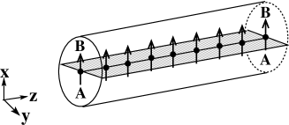
Stepanyan et al. used Equations (29) and (30), as the starting point of a self-consistent field calculation, adding conformational free energy contributions accounting for the entropy associated with the stretching of Gaussian chains. It is found that when exceeds a critical value , intramolecular phase separation of “Janus cylinder”-type occurs (Figure 14). Then an interface is formed, containing the backbone of the bottle brush, such that there is an excess of A-monomers below the interface and an excess of B-monomers above the interface (or vice versa). Assuming that at the position of the backbone the interface is oriented in x-direction, we can describe this Janus-type phase separation in terms of an one-dimensional order parameter density
| (31) |
where and are the numbers of A(B) monomers in the interval with and , respectively. Since we shall see below that the orientation of the interface is an important degree of freedom, we may consider as the absolute value of a vector order parameter , and the direction of is defined such that takes a maximum. However, Stepanyan et al. did not consider the possibility of an inhomogeneity along the z-axis, and they also did not derive how the order parameter depends on the parameters , , and the various parameters of the problem {Equation (29)}. Stepanyan et al. also assume that the distribution of chain ends is a delta function at the radius (or “height” ) respectively) of the bottle brush, where is given by in the good solvent regime. They then find that phase separation occurs for
| (32) |
but argue that this result holds only for a “marginal solvent” rather than a good solvent, due to the mean-field approximation used which neglects that inside a blob all binary contacts are avoided, estimating the number of contacts simply proportional to the product , cf. Equation (29), and neglecting the correlations due to excluded volume. The regime of marginal solvents is reached near the -point (which occurs for ), and requires that
| (33) |
where again prefactors of order unity are omitted.

Stepanyan et al. extend Equation (32) by a simple scaling-type argument, stating that the transition from the mixed state to the separated state occurs when the energy of the A-B contacts per side chain, , is of the order of . They estimate this energy as
| (34) |
where is the probability of the A-B contact, which depends on the average volume fraction of the monomers inside the brush. According to the mean field theory, , where , being the radius of the cylindrical brush. Using (Equation (8b)) one finds and using this result in Equation (34) implies , and from we recover Equation (32).
The merit of this simple argument is that it is readily extended to other cases: e.g., for a -solvent, we have and hence , yielding
| (35) |
For the poor solvent case, the bottle brush should collapse to a cylinder densely filled with monomers, and hence , , and thus
| (36) |
Note that Equation (36) is the same relation as for a dense bulk polymer blend or block copolymer melt, respectively.

The situation is more subtle in the good solvent case, however, since there the probability of contact is no longer given by the mean field result but rather by
| (37) |
where the Flory approximation was again used, with when . Equations (34) and (37) now imply
| (38) |
However, these crude estimates do not suffice to prove that for true long range order of this “Janus cylinder” type (Figure 14) is established. Hsu et al. suggested that there is also the need to consider variations of the direction of the order parameter along the z-direction (Figure 15). It was argued that for any finite side chain length also the cylinder radius (or brush “height”) is finite, and hence the system is one-dimensional. In one-dimensional systems with short range interactions at nonzero temperatures no long range order is possible. The situation depicted in Figure 15 is reminiscent of the one-dimensional XY-model of a chain of spins on a one-dimensional lattice where each spin at site is described by an angle in the xy-plane, with , and where neighboring spins are coupled. This coupling is described by the Hamiltonian
| (39) |
when is a unit vector in the xy-plane. While mean field theory predicts that ferromagnetic order occurs along the chain, for ferromagnetic exchange and temperatures less than the critical temperature which is of the order of , the exact solution of this model, Equation (39), shows that , since ferromagnetic long range order is unstable against long wavelength fluctuations. One can show that the spin-spin correlation function for large decays to zero exponentially fast,
| (40) |
where is the lattice spacing of this spin chain. The correlation length gradually grows as the temperature is lowered,
| (41) |
Equation (41) is at variance with mean field theory, which rather would predict (the index MF stands for “mean field” throughout)
| (42) |
This critical divergence at a nonzero critical temperature is completely washed out by the fluctuations: rather than diverging at , the actual correlation length {Equation (41)} at still is only of the order of the lattice spacing.
This consideration can be generalized to spin systems on lattices which have a large but finite size in dimensions and are infinite in one space dimensions only. E.g., when we consider an infinitely long cylinder of cross section we expect that Equations (41), (42) are replaced by the finite size scaling relation
| (43) |
where is the correlation length of the XY model on a lattice which is infinitely large in all directions of space.
| (44) |
where again (but with a smaller constant of proportionality than that in the relation , and is the correlation length exponent of the XY model (). Equation (43) describes a smooth crossover of the ferromagnetic correlation length describing spin correlations along the axis of the cylinder from bulk, Equation (44), to a quasi-one-dimensional variation. For the correlation length resembles Equation (41), since
| (45) |
the “helicity modulus” (also called “spin wave stiffness”) is of order for and shows a critical vanishing as from below, in the thermodynamic limit . However, for finite there is a finite size rounding of this singularity of , such that is of order , and hence a smooth crossover to Equation (43) occurs near . Figure 16 gives a qualitative account of this behavior. For more details of this finite size crossover we refer to the literature. But we suggest a qualitatively similar behavior for the domain size of segregated A-rich and B-rich domains in binary bottle brush polymers. So, when we study the correlation function of the order parameter considered in Equation (31)
| (46) |
we expect that the correlation length describing the local phase separation in the direction along the backbone of the bottle brush polymer remains of order unity as long as exceeds distinctly. For near we expect that becomes of order , the radius of the bottle brush. For , we expect , by analogy with Equation (45). Unfortunately, the test of those predictions even in the poor solvent case where is largest, is rather difficult, since the prefactor in the relation is unknown.

VI. Monte Carlo Results for Binary Bottle Brush Polymers
We use the same lattice model as considered before in our Monte Carlo study of the chain conformations of one-component bottle brush polymers, but now in the construction of the weights we have to take into account that the partition function now is
| (47) |
with (remember that we restrict attention to the choice
| (48) |
In Equation (47) the numbers of non-bonded occupied nearest-neighbor monomer pairs AA, BB and AB are denoted as and , respectively. Note that the sum in Equation (47) extends over all possible configurations of the bottle brush polymer. The choice corresponds to the previously studied one-component bottle brush under good solvent conditions, while the choice corresponds to variable solvent quality for the one-component brush (note that means , Equation (28), and also which is proportional to then vanishes: this means there is no chemical incompatibility between A and B any longer, no physical difference between A and B exists any more). From previous work on single chains we know that the -point occurs for . Therefore we varied in the range ; hence falls in the regime of poor solvent quality already. Of course, in order to have rather compact configurations of cylindrical bottle brushes a choice of much larger would be desirable. However, the efficiency of the PERM algorithm quickly deteriorates with increasing : for we encounter already for rather small values of the side chain length such as and a backbone length of huge statistical fluctuations. The total size of the bottle brush polymer under poor solvent conditions reached here, , is almost two orders of magnitude smaller than the maximal size studied under good solvent conditions! However, all known simulation algorithms for polymers suffer from difficulties of equilibration in the limit of very dense configurations.
Since we are mostly interested in the high grafting limit , so the number of side chains ) in the PERM algorithm where all side chains grow simultaneously we use a bias factor such that side chains are grown with higher probability in the directions perpendicular to the backbone. This additional bias (which is not present in the standard Rosenbluth and PERM methods) must be taken into account by suitable weight factors. About 106 independent configurations were typically generated.
Figures 17 - 19 now show typical results for the good solvent case but varying the parameter controlling the chemical incompatibility. The visual inspection of the configurations (Figure 17) reveals little influence of , however, and this observation is corroborated by the more quantitative analysis: the average number of A-B pairs per monomer is extremely small (Figure 18a) even for , and hence not much enthalpy could be won if A-chains and B-chains avoid each other: due to the excluded volume interaction, very few nearest neighbor contacts between any non-bonded monomers occur in our bottle brush model. For and the total number of AB contacts per chain is only about 1.4, and increases with increasing only very slowly. So for the range of side chain lengths accessible in our work, no phase separation should be expected. In the specific heat one does see a weak peak near , but the height of this peak decreases very strongly with increasing . Furthermore does neither the peak position shift with increasing (as one would expect from Equation (38), if this peak would be a rounded precursor of the phase transition that should occur at in the limit ) nor does the peak width decrease with increasing . Thus, it is clear that this peak is not an indicator of a “Janus-cylinder”-type phase separation in the bottle brush: rather we interpret it as a Schottky-type anomaly, expected from the fact that in our model of alternatingly grafted A-and B-chains at a straight line backbone with coordinates in the immediate environment of the backbone (e.g. at lattice sites or ) there is a nonzero a-priori probability of that between the first monomer of the chain grafted at and the first monomer of the chain grafted at a nearest-neighbor contact occurs. The finite energy from this local contacts near the backbone gives rise to the peak in the specific heat.
Also the radial density profile (Figure 19a) shows little effects of varying , and there is also no effect in the gyration radius component of the side chains, although a weak increase occurs in the corresponding component of the end-to-end distance (Figure 19b). In the latter figure, one can see for small an even-odd oscillation, but this lattice effect clearly has died out for .
In order to test for correlations measuring local phase separation along the backbone, Equation (46) is somewhat cumbersome to implement numerically, since for each one has to find the direction of from the condition that is maximal (cf. Equation (31)). A simpler and similar correlation function has been defined from the vectors pointing from the grafting site to the center of mass of the respective side chains. Projecting this vector into the xy-plane and defining an unit vector ( or ) along this projection (Figure 20) we define a correlation function as follows
| (49) |
Here we have explicitly incorporated the alternating grafting ABAB… of side chains along the backbone. The average in Equation (49) includes an averaging over all sites on which A chains are grafted, in order to improve the statistics. If perfect long range order occurs, as implied in Figure 20, we clearly have independent of , while for the case of short range order, we expect . Actually, considering the fact that we use a periodic boundary condition, we have analyzed our numerical data in terms of the ansatz
| (50) |
Figure 21 shows our data for for the three choices of : indeed we recognize that decays to zero with increasing , but the increase does get slower with increasing side chain length . The scale of this correlation effect clearly increases with decreasing . While for the correlation length hardly depends on , for large a slight increase of with decreasing is suggested.
In an earlier simulation study of phase separation in binary bottle brushes, it was suggested to quantify the degree of separation by considering the distribution of the polar angle from the axis to monomer . Defining a variable , which is if monomer is of type A and zero otherwise, and similarly , de Jong and ten Brinke introduced a function
| (51) |
and studied varying . However, it turns out that always has a rather complicated shape, and its dependence on is rather weak. Thus we investigated a related but somewhat different function, namely the histogram of the angle between the vectors from the axis to the centers of mass of subsequent unlike side chains (Figure 22). We see in this distribution also only a rather small dependence on , however: while for this distribution is essentially structureless for , for small a rather pronounced peak at develops, indicating a preference of antiparallel orientation of subsequent side chains. However, we feel that such indicators as or are sensitive only to the presence of short range order rather than long range order, and hence we shall focus on the correlation function in the following.
Next we focus on binary bottle brushes in a Theta solvent (. Figures 23 - 25 show that the results are not very different from the good solvent case: the average number of AB pairs per monomer (not shown) and the specific heat (Figure 23a) are hardly distinguishable from the good solvent case. Also the radial density profile (Figure 23b) exhibits only minor differences, slightly larger densities occur inside the brush than in the good solvent cases, and the transverse component of the end-to-end distance does not exhibit much additional stretching, when decreases (Figure 24a). The distribution is somewhat less flat near (Figure 24b) than in the good solvent case (Figure 22).
Also the correlation function shows again an exponential decay with (Figure 25a), the correlation length being rather similar to the good solvent case (Figure 21). Since one might argue that our definition of a correlation function as given in Equation (49) is not the optimal choice, and there might occur larger correlation lengths for a more clever choice of a correlation function, we tried a different choice which is also easy to compute. Namely, in the xy-plane at the index of the z-coordinate we determine the center of mass of the monomers of type or B in that plane (the choice of is dictated by the type of chain grafted at ). Then we introduce an unit vector from the z-axis in the direction towards this center of mass. In terms of these unit vectors, which then no longer distinguish from which chain the monomers in the ’th xy-plane are coming, we can again apply the definition, Equation (49) to derive a correlation function. This correlation function is shown in Figure 25b. One sees that the qualitative behavior of both types of correlation functions is the same, but the decay of this second type of correlation function even is slightly faster than that of the correlation function used previously. Since normally, when one studies problems involving a phase transition, the correlation length of the order parameter is the largest correlation length that one can find in the system, the previous definition (focusing on the location of the center of mass of the individual side chains) seems preferable to us. It is possible of course that such differences between different ways of measuring correlations along the backbone remain so pronounced for small only, where the correlation lengths are only of the order of a few lattice spacings, and hence are less universal and depend on the details of the studied quantity.
We now turn to the poor solvent case (Figures 26 - 29). Already the snapshot picture of the bottle brush polymer conformations (Figure 26) reveals that now the side chains adopt much more compact configurations, due to the collapse transition that very long single chains would experience in a poor solvent. If now becomes small, one recognizes a more pronounced phase separation along the backbone of the polymer, although there still is no long range order present.
Still, neither the variation of the average number of AB pairs per monomer with (Figure 27a) nor the specific heat (Figure 27b) give a hint for the occurrence of a phase transition: in fact, these data still look like in the good solvent case, Figure 18! Also the distribution and the variation of with and are qualitatively similar to the results found for good solvents and Theta solvents, and therefore are not shown here. More interesting is the monomer density profile (Figure 28). While for it still has the same character as in the previous cases, for and we recognize an inflection point. In fact, for a collapsed polymer bottle brush we expect a profile exhibiting a flat interior region at melt densities ( near to ), then an interfacial region where rapidly decreases towards zero; in the ideal case reached for , the profile should even be a Heaviside step function, in the continuum limit, . Obviously, for we are still far from this behavior even for , but we can identify an interface location at about , and in the interior of the cylindrical bottle brush (for ) the monomer density corresponds at least to a concentrated polymer solution.
Figure 29 then shows again plots of vs. , and the resulting fits to Equation (50). The behavior is qualitatively similar to the previous cases of good and Theta solvents again, but now the decay of with is clearly much slower, indicating a distinctly larger correlation length. This result corroborates the qualitative observation made already on the basis of the snapshot pictures, Figure 26, and quantifies it.
Our findings on the local character of phase separation in binary bottle brush polymers are now summarized in Figure 30, where plots of the inverse correlation length versus the inverse Flory-Huggins parameter are shown (cf. Equation (28) and remember our choice ). This choice of variables is motivated by the analogy with the XY model in cylindrical geometry, Equation (45); on the basis of this analogy, we would expect that , i.e. we expect straight lines that extrapolate through zero as .
Figure 30 demonstrates that this analogy clearly is not perfect. Rather the data are compatible with an extrapolation
| (52) |
where is a coefficient that decreases with increasing and depends on solvent quality and with a nonzero intercept implying that even in the ground state there is lack of long range order!
A very interesting question concerns the dependence of on chain length. Figure 31 presents a plot of , as estimated from extrapolation of the data shown in Figure 30 to , as a function of . Indeed the data are compatible with a relation , implying long range order for in the ground state. In principle, carrying out the same extrapolation at nonzero temperature and testing for which temperature range starts to be nonzero, one could obtain an estimate for the critical point of intramolecular phase separation, that should occur (and then is well defined) in the limit of infinite side chain length, . Unfortunately the accuracy of our estimates for does not warrant such an analysis.


The reason for this surprising persistence of disorder at low temperatures is configurational entropy, of course. As long as , the bottle brush polymer is not fully compact, and when the density is small enough inside the bottle brush (as it still is in the cases shown in Figure 28), the two types of chains A, B can avoid making binary contacts (as is evident from Figures 18 and 27): as . Hence there is a perfect avoidance of energetically unfavorable contacts in the ground state, and the finite correlation length and nonzero entropy of the ground state are not a consequence of “frustrated interactions” as in spin glasses, random field spin models, etc.. In the present problem, if both and are not too large, a ground state (for ) occurs where the structure of the bottle brush is NOT a cylinder with an interface separating an A-rich and a B-rich domain, as hypothesized in Figure 14! Thus a (coarse-grained) cross section of the bottle brush in the xy-plane is NOT a circle, separating A-rich and B-rich regions by a straight line, but rather looks like the number 8, i.e. a dumbbell-like shape, where a (more or less circular and more or less compact A-rich region) occurs for , a similar B-rich region occurs for , but no monomers (apart from the backbone monomer) occur at the y-axis at . The orientation of the x-axis can fluctuate as one moves along the z-axis, and unlike Figure 15 (twisting an interface in a cylinder along the z-axis clearly involves an energy cost, and this is described by the helicity modulus in the XY-model analogy, Equation (45)) the free energy cost of this structural distortion is outweighed by the configurational entropy gain, at least for and not too large. It is an unresolved question whether some critical value exists, where vanishes, and a long range ordered ground state occurs. Another unresolved question is, whether (another?) critical value exists, where the character of the ground state changes such that the local cross section of the binary bottle brush changes from an 8-shaped to a circular density distribution. Actually, the problem of alternatingly grafting A-chains and B-chains along a line is equivalent to grafting symmetric AB diblock copolymers along a line, such that the junction points of the diblocks form a straight line. This problem is the lower-dimensional analog of diblocks grafted with their junction points to the flat interface between an unmixed binary (A,B) homopolymer blend: for this problem it is well-known (see Werner et al. for references) that the shape of the diblocks is dumbbell like, the A-block being stretched away from the interface, in order to be embedded in the A-rich phase underneath of the interface, and the B-rich block also being stretched away from the interface, in order to be embedded in the B-rich phase above the interface.
As a consequence of our discussion, we call into question the idea of the “Janus cylinder”-type phase separation and propose as an alternative possibility (Figure 32) the “double cylinder” (with cross section resembling the number 8). Which of these cross-sectional structures occur will depend on the interaction parameters , and , of course. If the strength of the attractive interactions exceeds the strength of the repulsion sufficiently much, it is clear that for the Janus cylinder type phase separation will occur, while in the opposite limit, when exceeds sufficiently much, the double cylinder geometry will win. In the macroscopic continuum limit a comparison of the respective surface energies would imply that the double cylinder geometry, which avoids an AB interface, but requires for the same volume taken by A and B monomers a surface area of pure A and B that is larger by a factor of than for the “Janus cylinder” (Figure 32), becomes energetically preferable for
| (53) |
Since in the present work we consider the limit at fixed , it is clear that in our case Equation (53) is fulfilled. However, for the ”most symmetric” choice of interaction parameters, , the conclusion would be different. For lattice models Equation (53) is questionable since very compact configurations of collapsed polymers must respect the lattice structure, and different geometrical factors, depending on the type of the lattice, in the inequality Equation (53) may occur.
VII. Conclusions and Outlook
In this article, we have restricted attention exclusively to static conformational properties of very long bottle brush polymers with a rigid backbone. We feel that this “simple” limiting case needs to be understood first, before the very interesting extension to the case of flexible or semiflexible backbones, or the question of the crossover between a bottle brush polymer and a star polymer, can be correctly addressed. Thus the latter two problems were not at all considered in this paper, and hence we also do not wish to comment on the recent controversy concerning the correct interpretation of experiments on the overall linear dimensions of bottle brush polymers. Thus, the focus of the present article, as far as one-component bottle brush polymers are concerned, is the conformation of the side chains. We recall that this information is experimentally accessible, if one prepares bottle brushes with a single arm being deuterated, while all remaining arms of the polymer remain protonated, to allow a study of the static structure factor of a single arm by elastic coherent neutron scattering. It is clear that such experiments are very difficult, and hence no such experiment of this type is known to the present authors yet, but clearly it would be highly desirable to obtain such experimental information.
As discussed in the first part of the paper, one can find in the literature rather diverse concepts about the conformations of the side chains of a bottle brush polymer under good solvent conditions and high grafting density. One concept assumes that the cylindrical volume that the bottle brush occupies can be partitioned into disks, such that each disk contains just one polymer chain confined into it, no other chain participating in the same disk. A simple geometric consideration, reviewed in the first part of the present paper, then yields the following predictions for the linear dimensions of the chain, as a function of grafting density and side chain length
| (54) |
Remember that we choose the z-axis as the direction of the rigid backbone, the x-axis is oriented normal to the z-axis towards the center of mass of the chain, and the y-axis is perpendicular to both x- and z-axes. Thus the chain conformation has a quasi-two dimensional character, and there is no stronger stretching of a chain in radial direction than in tangential direction, since (independent of both and ).
Clearly, this quasi-two-dimensional picture is not very plausible, and more popular is an extension of the Daoud-Cotton blob picture for star polymers to the present case. While for a star polymer the blob radius simply increases proportional to the distance from the center, , and there is no geometrical difficulty to densely pack the conical compartments resulting from dividing a sphere into equal sectors, such that each sector contains a single arm of the star, with a sequence of spheres of increasing size, it has been argued in the literature that for cylindrical geometry the blob radius scales as . While in the literature no mentioning of a non-spherical blob shape (or, equivalently anisotropic local screening of the excluded volume interaction) is found, we have emphasized here the geometrically obvious fact that a dense filling of space with blobs in the cylindrical geometry appropriate for a bottle brush requires that the blobs have the shape of ellipsoids with three different axes, proportional to , , and , respectively. While this picture does not alter the prediction for the stretching of the chain in the radial x-direction found in the literature, , different predictions result for the other two linear dimensions. While the regular Daoud-Cotton picture would yield for the size of the last blob, , we find instead
| (55) |
| (56) |
Equations (55) and (56) make use of both the anisotropic blob linear dimensions and random walk-type arguments (cf. Equations (One- and two-component bottle-brush polymers: simulations compared to theoretical predictions)-(28)) and are new results, to the best of our knowledge.
Also the crossover scaling towards mushroom behavior has been considered, Equations (20)-(23), and Monte Carlo evidence for this crossover scaling description was obtained, from extensive work using the PERM algorithm. Although rather large bottle brushes were simulated (backbone length up to , avoiding free end effects by periodic boundary conditions, side chain length up to for grafting density , see Figure 2), it was not possible to reach the asymptotic regime of strong side chain stretching where Equations (55) and (56) hold, however. One reason why for moderate grafting densities even fairly long side chains can avoid each other with small significant amount of stretching is the fact that the natural shape of a self avoiding walk configuration is an elongated ellipsoid, with three rather different eigenvalues of the gyration tensor. So side chains can to a large extent avoid each other by orienting themselves such that the longest axis of the ellipsoid is oriented in the radial x-direction and the smallest axis in the backbone z-direction. This implies that very large values of are needed to obtain significant stretching. This difficulty to verify any such scaling laws in our simulations, which were only able to explore the onset of stretching away from simple mushroom-type behavior of the side chains and not the strongly stretched behavior, suggests that no such scaling behavior should be observable in the experiments as well: given the empirical fact that one bond of a coarse-grained lattice model corresponds to chemical monomers, it is clear that the experimentally accessible side chain lengths do not exceed those available in our simulation. Thus, scaling theories of bottle brushes are unfortunately of very restricted usefulness for the interpretation of either experiments or simulations. The only firm conclusion about the theories mentioned above that we like to make is that there is no evidence whatsoever for the quasi-two-dimensional picture, since we do see a decrease of with increasing .
Turning to the problem of intramolecular phase separation in binary (AB) bottle brush polymers, we have examined the proposal that a “Janus cylinder”-type phase separation occurs. This idea is questionable for several reasons (i) In a quasi-one-dimensional system, no sharp phase transition to a state with true long range order can occur; at most one can see a smooth increase in the corresponding correlation length, as the temperature is lowered (or the incompatibility between A and B is enhanced, respectively). Thus we have defined suitable correlation functions and studied the variation of the corresponding correlation length as function of the chain length and the parameter controlling the incompatibility ( is the repulsive energy encountered when two neighboring lattice sites are occupied by monomers of different kind). Three choices of solvent quality (taken symmetric for both A and B through the choice ) were considered, (good solvent), (Theta solvent) and (poor solvent). It was found that in all cases the correlation length suited to detect Janus-cylinder type ordering increases rather weakly as , approaching finite values even for , for finite side chain length , while for an infinite correlation length is compatible with the data. No evidence for the predicted critical points and their scaling behavior with (Equations 32-38) could be detected, however. The gradual establishment of a local phase separation lacking a sharp transition is compatible with observations from a previous simulation, however. (ii) Depending on the relation between the energy parameters and (cf. Equation (53)), the “local” phase separation (considering a slice of suitable thickness perpendicular to the backbone of the bottle brush to obtain suitable coarse-grained densities on mesoscopic scales) for temperatures may have two different characters (Figure 32a): the “Janus cylinder”, which contains an interface between A-rich and B-rich phases, competes with the “double cylinder”. In the latter structure, there is no extended AB interface, A-chains and B-chains meet only in the immediate vicinity of the backbone where they are grafted. Thus, the coarse-grained density distribution under poor solvent conditions in a slice has the shape of the number 8, where in the upper part of the 8 we have the B-rich phase and in the lower part we have the A-rich phase. Of course, when we orient the x-axis (Figure 14) such that it is parallel to the vector connecting the center of mass of the A-rich region to the center of mass of the B-rich region in the slice, the orientation of the x-axis for both structures in Figure 32 can randomly rotate when we move along the backbone (z-direction) due to long wavelength fluctuations, cf. Figure 15, and hence the comments about finite correlation lengths of this phase separation apply here as well. Actually, the numerical results of the present Monte Carlo simulations give clear evidence that local phase separation of “double cylinder”-type rather than “Janus cylinder” type is observed, since the number of AB-contacts tends to zero.
Thus, varying the solvent quality and chemical incompatibility, one can influence the character of local intramolecular phase separation, and one can control the correlation length over which the vector characterizing either interface orientation or the axis of the local dumbbell is oriented in the same way along the z-axis. Of course, in real systems one must expect that the solvent quality for the two types of chains will differ (Figure 32b). Then asymmetric 8-shaped local structures will result: e.g., if the solvent is a good solvent for B but a poor one for A, but the incompatibility between A and B is very high, we expect a structure where the A-chains are collapsed in a cylinder with the backbone on the cylinder surface, and from there the B-chains extend into the solution like a “flower” in the cross section (Figure 32b, left part). Conversely, it may happen that the solvent quality is poor for both A and B, but nevertheless different, so the densities of both cylinders and hence their radii will differ (Figure 32b, right part). Similar asymmetries are also of interest if the local character of the phase separation is of the Janus cylinder type: then in the cross section the A-rich and B-rich regions will take unequal areas, rather than equal areas as shown in Figure 32a, and the interface will be bent rather than straight. Similar effects will occur when the chain lengths differ from each other, or the flexibilities of both types of chains are different, etc.
An aspect which has not been discussed here but which is important for the binary bottle brush under poor solvent conditions is the question whether or not the density in the collapsed bottle brush is homogeneous along the z-direction (so one really can speak about “Janus cylinders” or “double cylinders”, Figure 32), or whether it is inhomogeneous so the state of the system rather is a chain of “pinned clusters”. For the one-component bottle brush, this question was discussed by Sheiko et al., from a scaling point of view, but (unlike the related problem of brush-cluster transition of planar brushes in good solvents) we are not aware of any simulation studies of this problem yet. In order to understand the structures of the binary bottle brush in the poor solvent, we count the number of monomers (irrespective of A or B) in each xy-plane, and calculate the normalized correlation function of along the backbone,
| (57) |
Here the average includes an averaging over all sites on which chains are grafted, in order to improve the statistics. In Figure 33, we see that this correlation actually is negative for , indicating some tendency to pinned cluster formation.
Before one can try to understand the real two-component bottle brush polymers studied in the laboratory, two more complications need to be considered as well: (i) the flexibility of the backbone; (ii) random rather than regular grafting along the sequence. While the effects due to (i) were already addressed to some extent in an earlier simulation, randomness of the grafting sequence has not been explored at all. However, in the study of binary brushes on flat substrates it has been found that randomness in the grafting sites destroys the long range order of the micro-phase separated structure, that is predicted to occur for a perfectly periodic arrangement of grafting sites. In the one-dimensional case, we expect the effects of quenched disorder in the grafting sites to be even more dominant than in these two-dimensional mixed polymer brushes. Hence, it is clear that the explanation of the structure of one- and two-component bottle brush polymers still is far from being complete, and it is hoped that the present article will motivate further research on this topic, from the point of view of theory, simulation and experiment.
Acknowledgement This work was financially supported by the Deutsche Forschungsgemeinschaft (DFG), SFB 625/A3. K. B. thanks S. Rathgeber and M. Schmidt for stimulating discussions and for early information about recent papers (Refs. 14 ; 15 ; 16 ). H.-P. H. thanks Prof. Peter Grassberger and Dr. Walter Nadler for very useful discussions. We are grateful to the NIC Jülich for providing access to the JUMP parallel processor.
References
- (1) A. Halperin, M. Tirrell, T. P. Lodge, Adv. Polym. Sci. 1991 100 31.
- (2) S. T. Milner, Science 1991, 251, 905.
- (3) G. S. Grest, M. Murat, “Monte Carlo and Molecular Dynamics Simulations in Polymer Science”, Ed. K. Binder, Oxford University Press, New York 1995, p. 476.
- (4) I. Szleifer, M. Carignano, Adv. Chem. Phys. 1996, 94, 165.
- (5) “Polymer Brushes”, R. C. Advincula, W. J. Brittain, K. C. Caster, J. Rühe, Eds., Wiley-VCH, Weinheim, 2004.
- (6) F. L. McCrackin, J. Mazur, Macromolecules 1981, 14, 1214.
- (7) J. E. L. Roovers, S. Bywater, Macromolecules 1972, 5, 384.
- (8) M. Daoud, J. P. Cotton, J. Phys. (Paris) 1982, 43, 531.
- (9) W. Burchard, Adv. Polym. Sci 1983, 48, 1.
- (10) T. M. Birshtein, E. B. Zhulina, Polymer 1984, 25, 1453.
- (11) T. M. Birshtein, E. B. Zhulina, O. V. Borisov, Polymer 1986, 27, 1078.
- (12) M. Wintermantel, M. Schmidt, Y. Tsukahara, K. Kajiwara, S. Kahjiya, Makromol. Chem., Rapid. Commun. 1994, 15, 279.
- (13) M. Wintermantel, M. Gerle, K. Fischer, M. Schmidt, I. Wataoka, H. Urakawa, K. Kajiwara, Y. Tsukahara, Macromolecules 1996, 29, 978.
- (14) S. Rathgeber, T. Pakula, A. Wilk, K. Matyjaszewski, K. L. Beers, J. Chem. Phys. 2005, 122, 124904.
- (15) S. Rathgeber, T. Pakula, A. Wilk, K. Matyjaszewski, H.-I. Lee, K. L. Beers, Polymer 2006, 47, 7318.
- (16) B. Zhang, F. Gröhn, J. S. Pedersen, K. Fisher, M. Schmidt, Macromolecules 2006, 39, 8440.
- (17) T. Witten, P. A. Pincus, Macromolecules 1986, 19, 2509.
- (18) T. M. Birshtein, O. V. Borisov, E. B. Zhulina, A. R. Khokhlov, T. A. Yurasova, Polym. Sci. USSR 1987, 29, 1293.
- (19) Z.-G. Wang, S. A. Safran, J. Chem. Phys. 1988, 89, 5323.
- (20) C. Ligoure, L. Leibler, Macromolecules 1990, 23, 5044.
- (21) R. C. Ball, J. F. Marko, S. T. Milner, T. A. Witten, Macromolecules 1991, 24, 693.
- (22) M. Murat, G. S. Grest, Macromolecues 1991, 24, 704.
- (23) N. Dan, M. Tirrell, Macromolecules 1992, 25, 2890.
- (24) C. M. Wijmans, E. B. Zhulina, Macromolecules 1993, 26, 7214.
- (25) H. Li, T. A. Witten, Macromolecules 1994, 27, 449.
- (26) E. M. Sevick, Macromolecules 1996, 29, 6952.
- (27) N. A. Denesyuk, Phys. Rev. E 2003, 67, 051803.
- (28) G. H. Fredrickson, Macromolecules 1993, 26, 2825.
- (29) E. B. Zhulina, T. A. Vilgis, Macromolecules 1995, 28, 1008.
- (30) Y. Rouault, O. V. Borisov, Macromolecules 1996, 29, 2605.
- (31) A. Yethiraj, J. Chem. Phys. 2006, 125, 204901.
- (32) M. Saariaho, O. Ikkala, I. Szleifer, I. Erukhimovich, G. ten Brinke, J. Chem. Phys. 1997, 107, 3267.
- (33) M. Saariaho, I. Szleifer, O. Ikkala, G. ten Brinke, Macromol. Theory Simul. 1998, 7, 211.
- (34) Y. Rouault, Macromol. Theory Simul. 1998, 7, 359.
- (35) M. Saariaho, A. Subbotin, I. Szleifer, O. Ikkala, G. ten Brinke, Macromolecules 1999, 32, 4439.
- (36) K. Shiokawa, K. Itoh, N. Nemoto, J. Chem. Phys. 1999, 111, 8165.
- (37) A. Subbotin, M. Saariaho, I. Ikkala, G. ten Brinke, Macromolecules 2000, 33, 3447.
- (38) P. G. Khalatur, D. G. Shirvanyanz, N. Y. Starovoitovo, A. R. Khokhlov, Macromol. Theory Simul. 2000, 9, 141.
- (39) S. Elli, F. Ganazzoli, E. G. Timoshenko, Y. A. Kuznetsov, R. Connolly, J. Chem. Phys. 2004, 120, 6257.
- (40) R. Connolly, G. Bellesia, E. G. Timoshenko, Y. A. Kuznetsov, S. Elli, F. Ganazzoli, Macromolecules 2005, 38, 5288.
- (41) S. Alexander, J. Phys. (Paris) 1977, 38, 983.
- (42) P. G. de Gennes, Macromolecules 1980, 13, 1069.
- (43) A. Halperin, “Soft Order in Physical Systems”, Ed. Y. Rabin, R. Bruinsma, Plenum Press, New York 1994, p. 33
- (44) P. J. Flory, “Principles of Polymer Chemistry”, Cornell Univ. Press, Ithaca, New York, 1953.
- (45) P. G. de Gennes, “Scaling Concepts in Polymer Physics”, Cornell University Press, Ithaca, New York, 1979.
- (46) P. Grassberger, Phys. Rev. E 1997, 56, 3682.
- (47) H.-P. Hsu, P. Grassberger, Europhys. Lett. 2004, 66, 874.
- (48) H.-P. Hsu, W. Nadler, P. Grassberger, Macromolecules 2004, 37, 4658.
- (49) H.-P. Hsu, W. Nadler, P. Grassberger, J. Phys. A: Math. Gen. 2005, 38, 775.
- (50) M. L. Huggins, J. Chem. Phys. 1941, 9, 440.
- (51) P. J. Flory, J. Chem. Phys. 1941, 9, 660.
- (52) K. Binder, Adv. Polymer Sci. 1994, 112, 181.
- (53) L. Leibler, Macromolecules 1980, 13, 1602.
- (54) I. W. Hamley, “The Physics of Block Copolymers”, Oxford University Press, New York, 1998.
- (55) G. H. Fredrickson, “The Equilibrium Theory of Inhomogeneous Polymers”, Oxford University Press, New York, 2006.
- (56) R. Stepanyan, A. Subbotin, and G. ten Brinke, Macromolecules 2002, 35, 5640.
- (57) J. de Jong, G. ten Brinke, Macromol. Theory Simul. 2004, 13, 318.
- (58) H.-P. Hsu, W. Paul, K. Binder, Europhys. Lett. 2006, 76, 526.
- (59) V. V. Vasilevskaya, A. A. Klochkov, P. G. Khalatur, A. R. Khokhlov, G. ten Brinke, Macromol. Theory Simul. 2001, 10, 389.
- (60) S. S. Sheiko, O. V. Borisov, S. A. Prokhorova, M. Möller, Eur. Phys. J. E. 2004, 13, 125.
- (61) P. G. Khalatur, A. R. Khokhlov, S. A. Prokhorova, S. S. Sheiko, M. Möller, P. Reineker, D. G. Shirvanyanz, N. Starovoltova, Eur. Phys. J. E 2000, 1, 99.
- (62) I. I. Potemkin, Eur. Phys. J. E 2003, 12, 207.
- (63) I. I. Potemkin, A. R. Khokhlov, S. Prokhorova, S. S. Sheiko, M. Möller, K. L. Beers, K. Matyijaszewski, Macromolecules 2004, 37, 3918.
- (64) J. C. Le Guillou, J. Zinn-Justin, Phys. Rev. B 1980, 21, 3976.
- (65) A. D. Sokal, “Monte Carlo and Molecular Dynamics Simulations in Polymer Science”, Ed. K. Binder, Oxford Univ. Press, New York, 1995, p. 47.
- (66) T. Kreer, S. Metzger, M. Müller, K. Binder, J. Baschnagel, J. Chem. Phys. 2004, 120, 4012.
- (67) S. T. Milner, T. A. Witten, M. Cates, Macromolecules 1988, 21, 2610.
- (68) A. M. Skvortsov, A. A. Gorbunov, I. V. Pavlushkov, E. B. Zhulina, O. V. Borisov, V. A. Priamitsyn, Polym. Sci USSR 1988, 30, 1706.
- (69) E. B. Zhulina, O. V. Borisov, V. A. Pryamitsyn, T. M. Birshtein, Macromolecules 1991, 24, 140.
- (70) J. Wittmer, A. Johner, J. F. Joanny, K. Binder, J. Chem. Phys. 1994, 101, 4379.
- (71) T. Cosgrove, T. Heath, B. van Lent, F. Leermakers, J. Scheutjens, Macromolecules 1987, 20, 1692.
- (72) C. M. Wijmans, J. M. H. M. Scheutjens, E. B. Zhulina, Macromolecules 1992, 25, 2657.
- (73) C. M. Wijmans, E. B. Zhulina, G. J. Fleer, Macromolecules 1994, 27, 3238.
- (74) R. R. Netz, M. Schick, Macromolecules 1998, 31, 5105.
- (75) M. Manghi, M. Aubouy, C. Gay, C. Ligoure, Eur. Phys. J. E 2001, 5, 519.
- (76) E. B. Zhulina, T. M. Birshtein, O. V. Borisov, Eur. Phys. J. E 2006, 20, 243.
- (77) M. Murat, G. S. Grest, Macromolecules 1989, 22, 4054.
- (78) A. Chakrabarti, R. Toral, Macromolecuels 1990, 23, 2016.
- (79) P. Y. Lai, K. Binder, J. Chem. Phys. 1991, 95, 9288.
- (80) G. S. Grest, M. Murat, Macromolecules 1993, 26, 3108.
- (81) G. S. Grest, Macromolecules 1994, 27, 418.
- (82) D. I. Dimitrov, A. Milchev, K. Binder, J. Chem. Phys. 2006, 125, 034905.
- (83) D. I. Dimitrov, A. Milchev, K. Binder, D. W. Heermann, Macromol. Theory Simul. 2006, 15, 573.
- (84) K. Kremer, K. Binder, Computer Phys. Repts. 1988, 7, 259.
- (85) K. Binder, “Monte Carlo and Molecular Dynamics Simulations in Polymer Science”, Ed. K. Binder, Oxford Univ. Press, New York 1995, p. 1.
- (86) K. Binder, J. Baschnagel, M. Müller, “Simulation Methods for Polymers”, Ed. M. J. Kotelyanskii, D. N. Theodorou, M. Dekker, New York 2004, p. 125.
- (87) H.-P. Hsu, P. Grassberger, AIP Conf. Proc. 2004, 690, 384.
- (88) H. Frauenkron, P. Grassberger, and W. Nadler, e-print cond-mat/9806321 1998.
- (89) H. Frauenkron, M. S. Causo, P. Grassberger, Phys. Rev. E 1999, 59, R16.
- (90) H.-P. Hsu, W. Nadler, P. Grassberger, Macromolecules 2004, 37, 4658.
- (91) M. N. Rosenbluth, A. W. Rosenbluth, J. Chem. Phys. 1955, 23, 356.
- (92) M. Doi, S. F. Edwards, “Theory of Polymer Dynamics”, Clarendon Press, Oxford, 1986.
- (93) D. Frenkel, G. C. A. M. Mooij, B. Smit, J. Phys.: Condens. Matter 1992, 4, 3053.
- (94) K. Ohno, K. Binder, J. Stat. Phys. 1991, 64, 781.
- (95) K. Ohno, T. Sakamoto, T. Minagawa, Y. Okabe, Macromlecules 2007, 40, 723.
- (96) I. Carmesin, K. Kremer, Macromolecules 1988, 21, 2819.
- (97) H.-P. Hsu, P. Grassberger, J. Chem. Phys. 2004, 120, 2034.
- (98) M. Daoud, P. G. de Gennes, J. Phys. (France) 1977, 38, 85.
- (99) A. Milchev, K. Binder, Eur. Phys. J. B 1998, 3, 477.
- (100) “Phase transitions and Critical Phenomena”, Vol 1. Eds. C. Domb, M. S. Green, Academic Press, New York, 1971.
- (101) R. J. Baxter, “Exactly Solved Models in Statistical Mechanics”, Academic Press, New York, 1982.
- (102) J. L. Richard, G. Sarma, J. Phys. C 1981, 14, L617.
- (103) M. E. Fisher, V. Privman, Phys. Rev. B 1975, 32, 477.
- (104) “Finite Size Scaling and Numerical Simulation of Statistical Systems”, Ed. V. Privman, World Scientific, Singapore, 1990.
- (105) K. Binder, “Computational Methods in Field Theory”, Eds. H. Gausterer, C. B. Lang, Springer, Berlin, 1992, p. 59.
- (106) J. Zinn-Justin, Phys. Repts. 2001, 344, 159.
- (107) K. Binder, A. P. Young, Rev. Mod. Phys. 1986, 58, 801.
- (108) K. Binder, W. Kob, “Glassy Materials and Disordered Solids. An Introduction to Their Statistical Mechanics”, World Scientific, Singapore, 2005.
- (109) A. Werner, F. Schmid, K. Binder, M. Müller, Macromolecules 1996, 29, 8241.
- (110) N. A. Desenyuk, Phys. Rev. E 2003, 68, 031803.
- (111) T. Stephan, S. Muth, M. Schmidt, Macromolecules 2002, 35, 9857.
- (112) C. Li, N. Gunari, K. Fischer, A. Janshoff, M. Schmidt, Angew. Chem. Int. Ed. 2004, 43, 1101.
- (113) L. Wenning, M. Müller, K. Binder, Europhys. Lett. 2005, 71, 639.
- (114) M. Müller, Phys. Rev. E 2002, 65, 030802.
- (115) P. Y. Lai, K. Binder, J. Chem. Phys. 1992, 97, 586.
- (116) G. S. Grest, M. Murat, Macromolecules 1993, 26, 3108.
- (117) C. Yeung, A. C. Balazs, D. Jasnow, Macromolecules 1993, 26, 1914.
- (118) H. Tang, I. Szleifer, Europhys. Lett. 1994, 28, 19.