Shallow decay phase of GRB X-ray afterglows from relativistic wind bubbles

Abstract

Aims. The postburst object of a GRB is likely to be a highly magnetized, rapidly rotating compact object (e.g., a millisecond magnetar), which could produce an ultrarelativistic electron-positron-pair wind. The interaction of such a wind with an outwardly expanding fireball ejected during the burst leads to a relativistic wind bubble (RWB). We investigate the properties of RWBs and use this model to explain the shallow decay phase of the early X-ray afterglows observed by Swift.

Methods. We numerically calculate the dynamics and radiative properties of RWBs.

Results. We find that RWBs can fall into two types: forward-shock-dominated and reverse-shock-dominated bubbles. Their radiation during a period of $\sim 10^{2}-10^{5}$ seconds is dominated by the shocked medium and the shocked wind, respectively, based on different magnetic energy fractions of the shocked materials. For both types, the resulting light curves always have a shallow decay phase, as discovered by Swift. In addition, we provide an example fit to the X-ray afterglows of GRB 060813 and GRB 060814 and show that they could be produced by forward-shock-dominated and reverse-shock-dominated bubbles, respectively. This implies that, for some early afterglows (e.g., GRB 060814), the long-lasting reverse shock emission is strong enough to explain their shallow decay phase.

1. Introduction

One of the most puzzling features of the early X-ray afterglow light curves of the gamma-ray bursts (GRBs) discovered by Swift (Gehrels et al. 2004) is the existence of a flattening segment (temporal indices $\alpha\sim[0,-0.8]$), which lasts from a few hundred seconds to a few hours (Campana et al. 2005; Vaughan et al. 2005; Cusumano et al. 2005; Nousek et al. 2006; O’Brien et al. 2006; de Pasquale et al. 2006; Willingale et al. 2006). This feature has been widely understood as due to a long-lasting energy injection. Two kinds of energy injection have been proposed. One kind is the so-called refreshed shock scenario with a smooth distribution of the Lorentz factors of the ejected shells (Rees & Mészáros 1998). The other kind, in focus here, involves a central engine activity extending over a long period (Dai & Lu 1998a, 1998b; Zhang & Mészáros 2001; Wang & Dai 2001; Dai 2004, D04 hereafter; Zhang et al. 2006; Fan & Xu 2006).

The popular models for the origin of long and short GRBs are the collapse of a massive star and merger of a compact binary, respectively (for recent reviews see Woosley & Bloom 2006; Nakar 2007). These models predict that, after a GRB, the remaining compact object seems to be a millisecond-period pulsar or a rapidly-rotating black hole. If the pulsar is strongly magnetized (e.g., a magnetar) or the black hole has an accretion disk lasting for a long time, these compact objects will continuously release their rotational energy through some magnetically-driven processes to produce an energy outflow. As this magnetically-driven outflow catches up to and then interacts with the relativistic fireball ejected during the GRB, the fireball’s energy will increase.

Based on this consideration, Dai & Lu (1998a, 1998b) and Zhang & Mészáros (2001) propose an energy-injection model for GRB afterglows with an assumption that the energy outflow is purely composed of low-frequency electromagnetic (EM) waves radiated by a postburst magnetar. Using this pure EM energy-injection (PEMI hereafter) model, Fan & Xu (2006) successfully explain the shallow decay phase of the X-ray afterglow of GRB 051221a. However, the numerical calculations (Wang & Dai 2001; Fan & Xu 2006) also show that an actual flattening segment of a light curve is steeper than an analytical estimation when the dynamics is numerically described and the equal-arrival surface effect is considered. Thus, it could be difficult to use the PEMI model to explain some GRB X-ray afterglows with a very flat plateau, such as GRB 060814.

On the other hand, the PEMI model does not consider possible evolution of the energy outflow with radius. Because the fluctuating component of the magnetic field in the outflow can in principle be dissipated by magnetic reconnection and used to accelerate an associated electron-positron plasma, the outflow should eventually become a kinetic-energy flow carried by the accelerated $\rm e^{\pm}$ pairs, even though it is dominated by the EM energy at small radii (Coroniti 1990; Michel 1994; Kirk & Skjæraasen 2003). This transformation of the outflow is estimated to occur around the radius $\sim 10^{7}r_{\rm L}-10^{9}r_{\rm L}$, that is, below the deceleration radius of the fireball ejected during the burst, where $r_{\rm L}$ ($\sim 10^{7}\rm cm$ for millisecond magnetars) is the light-cylinder radius of the pulsar. With these arguments, D04 suggests that it is likely to be an ultrarelativistic $e^{\pm}$-pair wind (but not pure EM waves) that interacts with the fireball to influence the GRB afterglow. As a result of the interaction, a relativistic wind bubble (RWB hereafter) is produced, which is a relativistic version of the Crab nebula.

In this paper, we calculate numerically the dynamic evolution and the corresponding radiation of a RWB driven by a millisecond magnetar by considering the inverse-Compton scattering effect and the equal-arrival surface effect of the RWB. Because of these effects, our numerical results are different from the analytical ones of D04. In particular, we find that RWBs fall into two types, which are dependent of the magnetic energy fractions of shocked materials. As an example, we fit the observed X-ray afterglows of GRB 060813 and GRB 060814, which are found to belong to two types of RWBs. We emphasize that, for some early afterglows (e.g., GRB 060814), the long-lasting reverse shock emission is strong enough to explain their shallow decay phase, which cannot be simulated by using the PEMI model.

2. Dynamics of a RWB

Some energy-source models (for a review see Zhang & Mészáros 2004) suggest that the central engine of a GRB is a millisecond magnetar. In such models, a GRB itself may be due to neutrino and/or magnetic processes of a rapidly-rotating, strongly-magnetized pulsar, which may eject a few shells. Collisions between the shells may produce internal shocks, which give rise to a few pulses of an observed GRB during the prompt emission. After the GRB, this pulsar will be braked by magnetic dipole radiation. As a result, the release of the stellar rotational energy (at a rate of $\dot{E}_{\rm rot}$) drives an outflow, whose luminosity is estimated by (Shapiro & Teukolsky 1983)

$$\begin{array}[]{ll}L_{\rm w}=-\dot{E}_{\rm rot}\\ \leavevmode\nobreak\ \leavevmode\nobreak\ \leavevmode\nobreak\ \leavevmode\nobreak\ \simeq 4.0\times 10^{47}B_{\perp,14}^{2}R_{\rm s,6}^{6}P_{0,\rm ms}^{-4}\left(1+{t\over T_{\rm sd}}\right)^{-2}\leavevmode\nobreak\ \rm erg\leavevmode\nobreak\ s^{-1},\end{array}$$ (1)

where $B_{\perp,14}=B_{\rm s,14}\sin\theta$, $\theta$ is the angle between the magnetic and rotational axes, and $B_{\rm s,14}=B_{\rm s}/10^{14}$G, $R_{\rm s,6}=R_{\rm s}/10^{6}\rm cm$, and $P_{0,\rm ms}=P_{0}/1$ms are the surface magnetic field strength, the radius, and the initial period of the magnetar, respectively. The time $t$ is measured in the observer’s frame. The characteristic spin-down time is $T_{\rm sd}\simeq 5.0\times 10^{4}(1+z)B_{\perp,14}^{-2}I_{45}R_{\rm s,6}^{-6}P_{0,\rm ms}^{2}\leavevmode\nobreak\ \rm s$, where $I_{45}=I/10^{45}\rm\leavevmode\nobreak\ g\leavevmode\nobreak\ cm^{2}$ is the stellar moment of inertia and $z$ the cosmological redshift. In the following calculations, the typical values of $R_{\rm s,6}$, $P_{0,\rm ms}$, and $I_{45}$ are all taken to be unity.

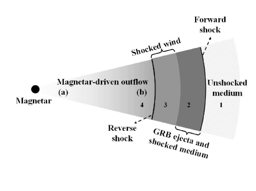
Figure 1: A schematic cartoon of an RWB. The meaning of the four regions (1-4) is explained in the text. In the inner (a) part of region 4, the energy outflow is dominated by low-frequency EM waves, in the outer (b) part of region 4 by a kinetic-energy flow carried by ultrarelativistic electron-positron pairs.

As the outflow propagates outward, the energy dissipation of the EM-wave component significantly accelerates plenty of associated $e^{\pm}$ pairs. Eventually, the outflow becomes an ultrarelativistic $e^{\pm}$-pair wind around some certain radius that is below the deceleration radius of the shells ejected during the burst. The wind’s bulk Lorentz factor is $\gamma_{\rm w}\sim 10^{4}-10^{7}$, as argued by Atoyan (1999) for the Crab pulsar. In the following calculations $\gamma_{\rm w}=10^{4}$. However, we find that a higher value of $\gamma_{\rm w}$ does not change our results significantly. As a result of interaction between the wind and the medium, an RWB should include two shocks: a reverse shock that propagates into the cold wind and a forward shock that propagates into the ambient medium. Here, for simplicity, we assume that two initially-forming forward shocks during the interaction of the GRB ejecta, both with the medium and with the wind, have eventually merged to one forward shock. Therefore, as illustrated in Fig. 1, there are four regions separated in the bubble by the shocks: (1) the unshocked medium, (2) the forward-shocked medium, (3) the reverse-shocked wind gas, and (4) the unshocked cold wind, where regions 2 and 3 are separated by a contact discontinuity.

We denote some quantities of region $i$ as follows: $n_{i}$ is the particle (proton or electron) number density and $P_{i}$ the pressure measured in its own rest frame, and $\gamma_{i}$ and $\beta_{i}=(1-\gamma_{i}^{-2})^{1/2}$ are the bulk Lorentz factor and corresponding velocity measured in the local medium’s rest frame, respectively. The total kinetic energy of region 2 is $E_{\rm K,2}=\gamma_{2}(m_{\rm ej}+m_{\rm sw})c^{2}+\gamma_{2}(\gamma_{2}-1)m_{\rm sw}c^{2}$, where $m_{\rm ej}$ is the rest mass of the initial GRB ejecta and $m_{\rm sw}$ is the rest mass of the swept-up medium. Energy conservation requires that any increase in $E_{\rm K,2}$ should be equal to work done by region 3: $dE_{\rm K,2}=\delta W=4\pi R^{2}P_{3}dR$, where $R$ is the radius of the bubble in the thin shell approximation. Then, we can obtain

$${d\gamma_{2}\over dR}={4\pi R^{2}\left[P_{3}/c^{2}-(\gamma_{2}^{2}-1)n_{1}m_{\rm p}\right]\over m_{\rm ej}+2\gamma_{2}m_{\rm sw}}.$$ (2)

On the other hand, the dynamic evolution of region 3 can be determined by the relationship between the Lorentz factors of the two sides of the contact discontinuity surface according to Blandford & McKee (1976)

$$\gamma_{3}=\gamma_{2}\chi^{-1/2},$$ (3)

where the similarity variable $\chi$ is (D04)

$$\chi=\left({L_{\rm w}\over 16\pi n_{1}m_{\rm p}c^{3}\gamma_{2}^{4}R^{2}}\right)^{-12/29},$$ (4)

where $m_{\rm p}$ is the proton rest mass. Using Eqs. 2, 3, 4, $P_{3}=L_{\rm w}/12\pi R^{2}\gamma_{3}^{2}c$ (D04), and the relations of $dt=(1+z)(1-\beta_{3})dR/\beta_{3}c$ for region 3 and $dt=(1+z)(1-\beta_{2})dR/\beta_{2}c$ for region 2, we can get the dynamic evolution of the RWB before the characteristic time $T_{\rm sd}$. Simultaneously, the masses of the shocked medium and shocked wind gas are calculated respectively by

$${dm_{\rm sw}\over dR}=4\pi R^{2}n_{1}m_{\rm p},$$ (5)

$${dm_{3}\over dR}=4\pi R^{2}(\beta_{4}-\beta_{\rm RS})\gamma_{4}n_{4}m_{\rm e},$$ (6)

where $m_{\rm e}$ is the electron rest mass and $\beta_{\rm RS}=(\gamma_{3}n_{3}\beta_{3}-\gamma_{4}n_{4}\beta_{4})/(\gamma_{3}n_{3}-\gamma_{4}n_{4})$ is the velocity of the reverse shock measured in the local medium’s rest frame. However, when $t>T_{\rm sd}$, the reverse shock is regarded as terminative (D04) and thus Eq. 3 should be replaced by $\gamma_{3}\propto R^{-7/2}$ (Kobayashi & Sari 2000; Kobayashi 2000), as well as $n_{3}\propto R^{-13/2},\leavevmode\nobreak\ P_{3}\propto R^{-26/3}$, and $dm_{3}=0$.

Figure 2 shows the evolution of the bulk Lorentz factors of regions 2 and 3 by taking the initial isotropic kinetic energy $E_{\rm K,2,0}=10^{51}\rm\leavevmode\nobreak\ ergs$ and the initial Lorentz factor $\gamma_{2,0}=150$ of region 2 at the deceleration radius, and $n_{1}=1\leavevmode\nobreak\ \rm cm^{-3}$. The shape of the curves is obviously consistent with the analysis in D04, who points out that the evolution can be divided into three stages: (I) $\gamma_{2}\propto t^{-3/8},\gamma_{3}\propto t^{-39/136}$; (II) $\gamma_{2}\sim\gamma_{3}\propto t^{-1/4}$; (III) $\gamma_{2}\propto t^{-3/8},\gamma_{3}\propto t^{-7/16}$.

Figure 2: The evolution of $\gamma_{2}$ and $\gamma_{3}$ in the RWB model with $B_{\perp,14}=2$ and $z=1$. The dotted curve represents the bulk Lorentz factor of the shocked medium without wind injection. The initial value of $\gamma_{2}$ is taken to be 150. This order of magnitude has been suggested by some observations (e.g., Molinari et al. 2006)

Compared with the case without wind injection, a significant change in the evolution of $\gamma_{2}$ is the existence of stage II, which is quite similar to the result of the PEMI model (Wang & Dai 2001). This similarity can be easily understood since the term $4\pi R^{2}P_{3}dR={2\over 3}(1+z)^{-1}L_{\rm w}dt$, which represents the work done by region 3 to region 2 in Eq. 2, is approximately equal to (strictly, a factor $2/3$ times) the term $(1+z)^{-1}L_{\rm w}dt$ in the dynamic equation of the PEMI model for the same magnetar (for details, see Dai & Lu 1998a, 1998b; Wang & Dai 2001; Fan & Xu 2006). Therefore, we cannot expect to distinguish the RWB model from the PEMI model only by observing the radiation from the forward-shocked medium. A possible difference between these two energy-injection models is induced by reverse-shocked pairs, the radiation of which arises from the remaining one-third energy release of the magnetar.

3. Radiation and example fit to X-ray afterglows

Both the forward shock and the reverse shock heat cold materials to a higher temperature, generate random magnetic fields, and accelerate protons and electrons. Since the microphysical processes have been unclear so far, the electron energy density and the magnetic energy density are parameterized as usual. We assume that for region 3 the electron and magnetic field energy densities are fractions $\epsilon_{\rm e,R}$ and $\epsilon_{\rm B,R}$ of the total energy density behind the reverse shock ($\epsilon_{\rm e,R}+\epsilon_{\rm B,R}=1$), and for region 2, fractions $\epsilon_{\rm e,F}$ and $\epsilon_{\rm B,F}$ of the total energy density behind the forward shock, where $\epsilon_{\rm e,F}+\epsilon_{\rm B,F}<1$ and $\epsilon_{\rm e,F}\sim\sqrt{\epsilon_{\rm B,F}}$ according to Medvedev (2006). It is natural to think that $\epsilon_{\rm B,R}\neq\epsilon_{\rm B,F}$ and $\epsilon_{\rm e,R}\neq\epsilon_{\rm e,F}$, as suggested in some studies (Fan et al. 2002; Coburn & Boggs 2003; Zhang, Kobayashi & Mészáros 2003; Kumar & Panaitescu 2003). We also assume that the spectral indices of the electron energy distribution are $p_{2}$ and $p_{3}$ for regions 2 and 3, respectively. Furthermore, we assume here that $p_{2}\sim p_{3}=p$. By giving a set of three free parameters ($p,\leavevmode\nobreak\ \epsilon_{\rm B,F}$ and $\epsilon_{\rm B,R}$), we can fix the cooling Lorentz factors $\gamma_{\rm e,c}$ arising from both synchrotron radiation and inverse-Compton scattering, and the minimum Lorentz factors $\gamma_{\rm e,min}$ in the electron energy distributions of regions 2 and 3. We also consider the “equal-arrival surface” effect of the RWB emission. The related formulas for these calculations were presented in Sect. 3 of Huang et al. (2000). We ignore the self-absorption effect for the X-ray emission we are interested in.

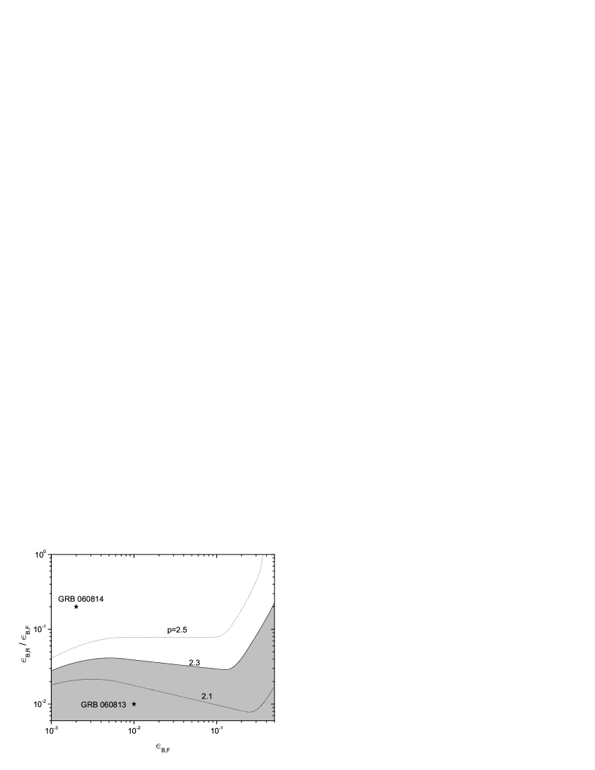
Figure 3: Parameter space of $(p,\leavevmode\nobreak\ \epsilon_{\rm B,F},\leavevmode\nobreak\ \epsilon_{\rm B,R})$ with $B_{\perp,14}=2$ and $z=1$. The lines represent the critical values $(\epsilon_{\rm B,R}/\epsilon_{\rm B,F})_{\rm c}$ with different $p$, below which ( in the shaded area for $p=2.3$) the corresponding reverse shock emission is insignificant for the total flux of the RWB. The star symbols label the parameter sets of two GRBs.

Before light curves are exhibited, it should be pointed out that the ratio of the flux contributed by regions 2 or 3 to the total flux is sensitive to the ratio of $\epsilon_{\rm B,R}/\epsilon_{\rm B,F}$. As shown in Fig. 3, if a dot representing a parameter set $(p,\leavevmode\nobreak\ \epsilon_{\rm B,F},\leavevmode\nobreak\ \epsilon_{\rm B,R})$ is in the shaded area (for $p=2.3$), the peak of the light curve of the reverse shock emission is below the light curve of the forward shock emission (e.g., see the upper panel of Fig. 4). The higher the value of $p$, the easier the occurrence of this case. Because the forward shock dominates the radiation of the RWB, as discussed above, the combined light curve should be similar to the result of the PEMI model for an identical magnetar. In other words, all the GRB X-ray afterglows that can be fitted in the PEMI model must be explained by the RWB model with an appropriate parameter set. Conversely, if $\epsilon_{\rm B,R}/\epsilon_{\rm B,F}$ is large enough ($>(\epsilon_{\rm B,R}/\epsilon_{\rm B,F})_{\rm c}$), the radiation from region 3 becomes quite important, especially during a period of $\sim 10^{2}-10^{5}\,$s. Therefore, we can divide the RWBs into two types: forward-shock-dominated and reverse-shock-dominated bubbles.

However, because of the existence of stage II in the dynamic evolution, the afterglows produced by two types of RWBs always have a shallow decay phase. This feature of RWBs is very consistent with a lot of afterglows observed by Swift. For example, two X-ray afterglows of GRB 060813 (upper panel) and GRB 060814 (lower panel) are fitted by the RWB model as shown in Fig. 4, and the corresponding parameter sets $(p,\leavevmode\nobreak\ \epsilon_{\rm B,F},\leavevmode\nobreak\ \epsilon_{\rm B,R})$ are shown in Fig. 3. It can clearly be suggested that the afterglows of GRB 060813 and GRB 060814 could be produced by forward-shock-dominated and reverse-shock-dominated RWBs, respectively. As discussed above, the prompt emission of a GRB may result from internal shocks. If the high-latitude emission of the last internal shocks is weaker than the early afterglow emission, one can observe the shallow decay of an early afterglow, as in GRB 060813. Conversely, an early steep decay should be observed (Kumar & Panaitescu 2000), as in GRB 060814. For the latter burst, we should thus introduce this curvature effect to explain the earlier steep decay, which is fitted roughly by the following equation (as shown in the inserting panel of Fig. 4, also see Zhang et al. 2006; Liang et al. 2006):

$$F_{\rm X}(t)=A\left({t-t_{0}\over t_{0}}\right)^{-(2+\beta)}+F_{\rm X,RWB},$$ (7)

where $A$ is the normalization parameters, $t_{0}$ the time zero point of the last prompt emission pulse, and $\beta$ the spectral index that is equal to 0.67 (Moretti, Guidorzi & Romano 2006). Please note that we take the time zero point of the afterglow as the GRB triggering time as proved by Kobayashi & Zhang (2006) and Liang et al. (2006).

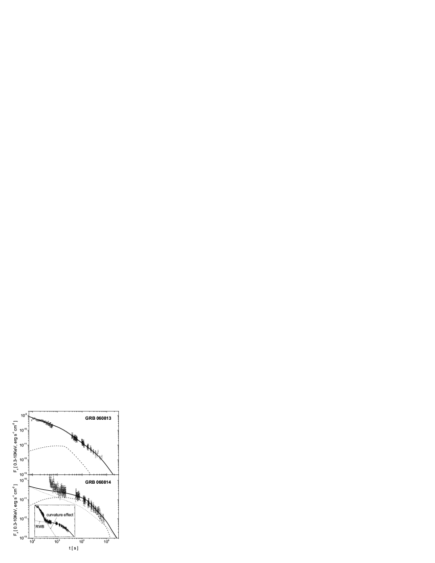
Figure 4: Fits of GRB 060813 with $B_{\perp,14}=6.5,p=2.5,\epsilon_{\rm B,F}=0.01,\epsilon_{\rm B,R}=0.0001,z=0.6$, and GRB 060814 with $B_{\perp,14}=2.5,p=2.2,\epsilon_{\rm B,F}=0.002,\epsilon_{\rm B,R}=0.0004,z=0.6$ using the RWB model. The half-opening angles of jets are $\theta_{j}=0.1$ and $\theta_{j}=0.15$, respectively. The solid lines correspond to total fluxes, while the dotted and dashed lines represent the fluxes determined by the forward and reverse shocks, respectively. The early steep decay segment of GRB 060814 is fitted with $A=9.85\times 10^{-9}\rm\leavevmode\nobreak\ erg\leavevmode\nobreak\ s^{-1}cm^{-2}$ and $t_{0}=75\leavevmode\nobreak\ \rm s$ in the insert.

4. Summary

In this paper, we have numerically calculated the dynamic evolution and radiation of RWBs. Two motivations impel us to consider this RWB model rather than the PEMI model: first, the PEMI model cannot explain the very flat plateau in light curves of some X-ray afterglows; second, a pulsar-driven energy outflow, which is dominated by Poynting flux at smaller radii, could evolve into an ultrarelativistic electron-positron-pair wind at larger radii. The most significant feature of the light curves of the X-ray afterglows from the RWBs is a flattening segment occurring during a period of $\sim 10^{2}-10^{5}\,$s, which is consistent with the observed shallow decay phase. Our example fits to the X-ray afterglows of GRB 060813 and GRB 060814 indicate that they could be produced by forward-shock-dominated and reverse-shock-dominated RWBs, respectively. This suggests that the central engines of these two GRBs could be millisecond magnetars. Moreover, the example fits also show that, besides the X-ray afterglows that can be fitted in the PEMI model (e.g., GRB 060813), the RWB model can also explain some other afterglows with a very flat plateau (e.g., GRB 060814) that create difficulties for the PEMI model.

In addition, we would like to point out that the magnetar-driven RWB model is one possibility. As pointed out in the introduction and in D04, RWBs could also be produced, in principle, by central black holes that accrete circumburst materials after the GRB. Moreover, some other models have also been proposed to explain the observed shallow decay phase, e.g., off-beam jets, two-component jets, and varying microphysics parameters (Eichler & Granot 2006; Granot et al. 2006; Panaitescu et al. 2006; also see Zhang 2007 for a recent review). It is a demanding task to distinguish between the above models by using multiwavelength observations.

- (1) Atoyan A. M. 1999, A&A, 346, L49
- (2) Blandford R. D. & McKee C. F. 1976, Phys. Fluids., 19, 1130
- (3) Campana S. et al. 2005, ApJ, 625, L23
- (4) Coburn W. & Boggs, S. E. 2003, Nature, 423, 415
- (5) Coroniti F. V. 1990, ApJ, 349, 538
- (6) Cusumano G., et al. 2005, ApJ, 639, 316
- (7) Dai Z. G. 2004, ApJ, 606, 1000 (D04)
- (8) Dai Z. G. & Lu T. 1998a, A&A, 333, L87
- (9) Dai Z. G. & Lu T. 1998b, Phys. Rev. Lett., 81, 4301
- (10) de Pasquale M. et al. 2006, MNRAS, 365, 1031
- (11) Eichler D. & Granot J. 2006, ApJ, 641, L5
- (12) Fan Y. Z., Dai Z. G., Huang Y. F. & Lu T. 2002, ChJAA, 2, 449
- (13) Fan Y. Z. & Xu D. 2006, MNRAS, 372, L19
- (14) Gehrels N. 2004, ApJ, 611, 1005
- (15) Granot J., Knigl A. & Piran T. 2006, MNRAS, 370, 1946
- (16) Huang Y. F., Gou L. J., Dai Z. G. & Lu T. 2000, ApJ, 543, 90
- (17) Kirk J. G. & Skjæaasen, O. 2003, ApJ, 591, 366
- (18) Kobayashi S. 2000, ApJ, 545, 807
- (19) Kobayashi S. & Sari R. 2000, ApJ, 542, 819
- (20) Kobayashi S. & Zhang B. 2007, ApJ, 655, 973
- (21) Kumar P. & Panaitescu A. 2000, ApJ, 541, L51
- (22) Kumar P. & Panaitescu A. 2003, MNRAS, 346, 905
- (23) Liang E. W. et al. 2006, ApJ, 646, 351
- (24) Medvedev M. V. 2007, ApJ, 654, 764
- (25) Michel F. C. 1994, ApJ, 431, 397
- (26) Molinari E. et al. 2006, arXiv: astro-ph/0612607
- (27) Moretti A., Guidorzi C. & Romano P. 2006, GCN 5451
- (28) Nakar E., 2007, Phys. Rep. (Bethe Centennial Volume), arXiv: astro-ph/0701748
- (29) Nousek J. A. et al. 2006, ApJ, 642, 389
- (30) O’Brien P. T. et al. 2006, ApJ, 647, 1213
- (31) Panaitescu A. & P. et al. 2006, MNRAS, 369, 2059
- (32) Rees M. J. & P. 1998, ApJ, 496, L1
- (33) Shapiro S. L. & Teukolsky S. A. 1983, Black Holes, White Dwarfs, and Neutron Stars, NY: John Wiley & Sons, 278
- (34) Vaughan S. et al. 2005, ApJ, 638, 920
- (35) Wang W. & Dai Z.G. 2001, Chin. Phys. Lett., 18, 1153
- (36) Willingale R., 2006, submitted to ApJ, arXiv: astro-ph/0612031
- (37) Woosley S.E. & Bloom J.S., 2006, ARA&A, 44, 507
- (38) Zhang B. 2007, ChJAA, 7, 1
- (39) Zhang B. et al. 2006, ApJ, 642, 354
- (40) Zhang B., Kobayashi S. & P. 2003, ApJ, 595, 950
- (41) Zhang B. & P. 2001, ApJ, 552, L35
- (42) Zhang B. & P. 2004, IJMPA, 19, 2385