Controllability of the coupled spin-half harmonic oscillator system

Abstract

We present a control-theoretic analysis of the system consisting of a two-level atom coupled with a quantum harmonic oscillator. We show that by applying external fields with just two resonant frequencies, any desired unitary operator can be generated.

I Introduction

In this paper, we apply theoretical concepts of quantum control to the joint system consisting of a two state system coupled with a quantum harmonic oscillator. Such systems are ubiquitous in Nature. For example, coupled atom-oscillator systems form the basis for the ion trap quantum computerCZ95 . Other examples include a single atom in a cavityKimble , a super-conducting qubit in a cavityWall , and control of single atom lasersCarm ; Mcke . In Law , Law and Eberly showed that arbitrary states can be synthesized by using just two resonant frequencies, a result experimentally verified in Wineland03 , and Rangan showed that the two-level atom-oscillator system could be controlled by fine-tuning the Lamb-Dicke parameter. Here we prove that the dynamics of such systems is controllable without any fine-tuning or special state preparation: with the proper sequence of pulses, it is possible to perform any desired unitary transformation on the Hilbert space spanned by the atomic states together with the lowest $n$ energy levels of the oscillator.

In this paper, we will use the ion trap as our model system. An ion trap quantum computer can be modeled as a collection of $N$ particles with spin $1\over 2$ in a one-dimensional harmonic potential. Laser pulses incident on the ions can be tuned to simultaneously cause internal spin transitions and vibrational (phonon) excitations, thus allowing local internal states to be mapped into shared phonon states. The computational qubits are encoded by two internal states of each ion and the collective vibration of the trapped ions acts as the information bus. In this manner, quantum information can be communicated between any pair of ions and logic gates can be performed. Several key features of the original proposal in CZ95 , including the production of entangled states and the implementation of quantum controlled operations between a pair of trapped ions, have already been experimentally demonstrated (see, e.g., Monroe95 ; King98 ; Turchette98 ; Sackett00 ). Meanwhile, several alternative theoretical schemes (see, e.g., Duan01 ; Jonathan01 ; wei02 ; Jonathan00 ; Childs01 ; Rangan ) have also been developed for overcoming various difficulties in realizing a practical ion-trap quantum information processor. All these proposals either require fine-tuning of the Lamb-Dicke parameter or an initial eigenstate of the vibration motion. Here we present a control theoretical analysis and show that in the Lamb-Dicke regime by using two resonant frequencies, any unitary transformation within a finite level of the harmonic oscillator can be generated. Unlike, e.g., Rangan , no fine-tuning of the Lamb-Dicke parameter is required to obtain complete control. While the proof of controllability is somewhat involved, because of the fundamental nature of the system to be controlled and because of the wide range of potential application, we present this proof in detail. As will be seen below, the difficulty of the proof arises because, in the absence of controllability of the Lamb-Dicke parameter, one must combine discrete and continuous control theoretic techniques. The current proof can be regarded as extending the techniques of the paperChilds01 ; Chuang03 from controlling 4 states to controlling $m$ states, where $m$ can be arbitrary large. We begin in section II by presenting the usual Jaynes-Cumming model for spin boson interaction. We then make the controllability analysis of the system in section III.

II Laser-ion interaction model

The physical situation we consider is a two-state atom (frequency $\omega_{c}$) coupled to a harmonic oscillator (transition frequency $\omega_{z}$), driven additionally by an external field (frequency $\omega$). We will follow the ion trap model Win97 ; Childs01 . The free Hamiltonian of this system is $H_{0}=\hbar\omega_{c}{\sigma_{z}\over 2}+\hbar\omega_{z}a^{\dagger}a$, where $\sigma_{z}$ is a Pauli spin operator and $a$ annihilates a phonon. Turning on the electromagnetic field of a laser gives an interaction Hamiltonian

$$H_{I}=-\vec{\mu}\cdot\vec{B}\,,$$ (1)

where $\vec{\mu}=\mu\vec{\sigma}/2$ is the magnetic moment of the ion and $\vec{B}=B\hat{x}\cos(kz-\omega t+\Phi)$ is the magnetic field produced by the laser. Here $z=z_{0}(a+a^{\dagger})$, where $z_{0}=\sqrt{\hbar/2Nm\omega_{z}}$ is a characteristic length scale for the motional wave functions and $m$ is the mass of an ion.

We consider the regime in which $\eta\equiv kz_{0}\ll 1$. In this regime, we may determine the effect of a laser pulse at a specific frequency $\omega$ by expanding Eq. (1) in powers of $\eta$ and neglecting rapidly rotating terms. Then pulsing on resonance ($\omega=\omega_{c}$) allows one to perform the transformation

$$R(\theta,\phi)=\exp\left[i{\theta}(e^{i\phi}\sigma^{+}+e^{-i\phi}\sigma^{-})\right]\,,$$ (2)

and pulsing at the red sideband frequency ($\omega=\omega_{c}-\omega_{z}$) gives

$$R^{-}(\theta,\phi)=\exp\left[i{\theta}(e^{i\phi}\sigma^{+}a^{\dagger}+e^{-i\phi}\sigma^{-}a)\right]\,.$$ (3)

In each case, the parameter $\theta$ depends on the strength and duration of the pulse and $\phi$ depends on its phase.

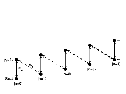
Figure 1: Graphical representation of the quantum harmonic oscillator driven by a sinusoidal resonant field fields $\omega_{c}$ and $\omega_{r}=\omega_{c}-\omega_{z}$ as shown. The strengths of the $\omega_{c}$ transition couplings are independent of the harmonic oscillator quantum number $n$, whereas the strength of the $\omega_{r}$ transition couplings increase as the square root of the quantum number $n$.

In the next section, we show that by just using these two frequencies any unitary operator can be generated. The basic idea in proving controllability is an extension of Childs01 ; Chuang03 . Using the feature that the transition frequencies increase as the square root of the quantum number, we apply only pulses that leave the system confined within the Hilbert space spanned by the first $n$ oscillator levels. This requirement means that the only a discrete set of pulses can be applied at the red sideband frequency. Meanwhile, a continuous set of pulses can be applied at the resonance frequency. As a result of the use of both discrete and continuous controls, the resulting control problem is technically somewhat involved. Nonetheless, it can be solved completely, as we now show.

III Controllability analysis

We denote $E_{pq}$ be the matrix such that has all the entries equal to zero except the $pq$ entry, which equals $1$. It is easy to check that $E_{pq}E_{rs}=\delta_{q}^{r}E_{ps}$.

The Hamiltonian, after absorbing the imaginary number $i$, can be represented as skew-Hermitian matrices. If we take the eigen-state of the free Hamiltonian as the basis, then after re-scaling the time unit, the various Hamiltonians in the interaction frame can be represented as

1) $\omega=\omega_{c}$, $\phi=0$

$$\begin{aligned} H_{1}&=i\sum_{k=0}^{\infty}E_{(2k+1)(2k+2)}+E_{(2k+2)(2k+1)}\\ &=i\left[\begin{array}[]{ccccccc}0&1&0&0&0&0&...\\ 1&0&0&0&0&0&...\\ 0&0&0&1&0&0&...\\ 0&0&1&0&0&0&...\\ 0&0&0&0&0&1&...\\ 0&0&0&0&1&0&...\\ \vdots&\vdots&\vdots&\vdots&\vdots&\vdots&\vdots\\ \end{array}\right]\,,\end{aligned}$$ (4)

2) $\omega=\omega_{c}$, $\phi=\frac{\pi}{2}$,

$$\begin{aligned} H_{2}&=\sum_{k=0}^{\infty}E_{(2k+1)(2k+2)}-E_{(2k+2)(2k+1)}\\ &=\left[\begin{array}[]{ccccccc}0&1&0&0&0&0&...\\ -1&0&0&0&0&0&...\\ 0&0&0&1&0&0&...\\ 0&0&-1&0&0&0&...\\ 0&0&0&0&0&1&...\\ 0&0&0&0&-1&0&...\\ \vdots&\vdots&\vdots&\vdots&\vdots&\vdots&\vdots\\ \end{array}\right]\,,\end{aligned}$$ (5)

3) $\omega=\omega_{c}-\omega_{z}$, $\phi=0$,

$$\begin{aligned} H_{3}&=i\sum_{k=1}^{\infty}\sqrt{k}\left[E_{(2k)(2k+1)}+E_{(2k+1)(2k)}\right]\\ &=i\left[\begin{array}[]{ccccccc}0&0&0&0&0&0&...\\ 0&0&1&0&0&0&...\\ 0&1&0&0&0&0&...\\ 0&0&0&0&\sqrt{2}&0&...\\ 0&0&0&\sqrt{2}&0&0&...\\ 0&0&0&0&0&0&...\\ \vdots&\vdots&\vdots&\vdots&\vdots&\vdots&\vdots\\ \end{array}\right].\end{aligned}$$ (6)

4) $\omega=\omega_{c}-\omega_{z}$, $\phi=\frac{\pi}{2}$,

$$\begin{aligned} H_{4}&=\sum_{k=1}^{\infty}\sqrt{k}\left[E_{(2k)(2k+1)}-E_{(2k+1)(2k)}\right]\\ &=\left[\begin{array}[]{ccccccc}0&0&0&0&0&0&...\\ 0&0&1&0&0&0&...\\ 0&-1&0&0&0&0&...\\ 0&0&0&0&\sqrt{2}&0&...\\ 0&0&0&-\sqrt{2}&0&0&...\\ 0&0&0&0&0&0&...\\ \vdots&\vdots&\vdots&\vdots&\vdots&\vdots&\vdots\\ \end{array}\right].\end{aligned}$$ (7)

When the Hamiltonian $H_{3}$ or $H_{4}$ is applied, $|\uparrow\rangle|m\rangle$ is connected to $|\downarrow\rangle|m+1\rangle$. We restrict the evolution time $T$ under these two Hamiltonian to satisfy $T\sqrt{m}=k\pi$, while $k$ is integer, so the subspace of states spanned by $\{|\downarrow,\uparrow\rangle|j\rangle|j\leq m\}$ is preserved. We show that under these restrictions any unitary matrix within any finite harmonic level still can be generated.

III.1 $SU(4)$

Let’s first work out the case of $m=1$, show that we can generate $SU(4)$ on the subspace spanned by states

$$|\downarrow\rangle|0\rangle,|\uparrow\rangle|0\rangle,|\downarrow\rangle|1\rangle,|\uparrow\rangle|1\rangle$$

Restricted to this subspace,

$$H_{1}=i\left[\begin{array}[]{cccc}0&1&0&0\\ 1&0&0&0\\ 0&0&0&1\\ 0&0&1&0\\ \end{array}\right]\,,$$

$$H_{2}=\left[\begin{array}[]{cccc}0&1&0&0\\ -1&0&0&0\\ 0&0&0&1\\ 0&0&-1&0\\ \end{array}\right]\,,$$

and the unitary operators we can generate using $H_{3}$ and $H_{4}$ are

$$\begin{aligned} R^{-}(\frac{k\pi}{\sqrt{2}},0)&=\exp\left[\frac{k\pi}{\sqrt{2}}H_{3}\right]\\ &=\left[\begin{array}[]{cccc}1&0&0&0\\ 0&\cos(\frac{k\pi}{\sqrt{2}})&i\sin(\frac{k\pi}{\sqrt{2}})&0\\ 0&i\sin(\frac{k\pi}{\sqrt{2}})&\cos(\frac{k\pi}{\sqrt{2}})0&0\\ 0&0&0&(-1)^{k}\\ \end{array}\right]\,,\end{aligned}$$ (8)

$$\begin{aligned} R^{-}(\frac{k\pi}{\sqrt{2}},\frac{\pi}{2})&=\exp\left[\frac{k\pi}{\sqrt{2}}H_{4}\right]\\ &=\left[\begin{array}[]{cccc}1&0&0&0\\ 0&\cos(\frac{k\pi}{\sqrt{2}})&\sin(\frac{k\pi}{\sqrt{2}})&0\\ 0&-\sin(\frac{k\pi}{\sqrt{2}})&\cos(\frac{k\pi}{\sqrt{2}})&0\\ 0&0&0&(-1)^{k}\\ \end{array}\right]\,,\end{aligned}$$ (9)

Choose $k=2p$, by varying $p$, $R^{-}(\frac{k\pi}{\sqrt{2}},\frac{\pi}{2})$ forms a dense subset of the one parameter group

$$e^{t\left[\begin{array}[]{cccc}0&0&0&0\\ 0&0&1&0\\ 0&-1&0&0\\ 0&0&0&0\\ \end{array}\right]}$$

Thus we have the generator $\left[\begin{array}[]{cccc}0&0&0&0\\ 0&0&1&0\\ 0&-1&0&0\\ 0&0&0&0\\ \end{array}\right]$, add it to $H_{2}$, we get

$$H_{5}=\left[\begin{array}[]{cccc}0&1&0&0\\ -1&0&1&0\\ 0&-1&0&1\\ 0&0&-1&0\\ \end{array}\right]$$

Choose $k=2p+1$, we can have

$$\begin{aligned} U_{1}&=R^{-}(\frac{k\pi}{\sqrt{2}},\frac{\pi}{2})\\ &=\left[\begin{array}[]{cccc}1&0&0&0\\ 0&\cos(\frac{k\pi}{\sqrt{2}})&\sin(\frac{k\pi}{\sqrt{2}})&0\\ 0&-\sin(\frac{k\pi}{\sqrt{2}})&\cos(\frac{k\pi}{\sqrt{2}})&0\\ 0&0&0&-1\\ \end{array}\right]\,,\end{aligned}$$ (10)

Since $U(4)$ is compact, the infinite sequence $\{U_{1},U_{1}^{2},U_{1}^{3},U_{1}^{4}...\}$ has a convergent subsequence, i.e., there exists $p_{1}>p_{2}\in N$ such that $U_{1}^{p_{1}}-U_{1}^{p_{2}}$ is arbitrary close to zero, when this is true then $U_{1}^{p_{1}-p_{2}-1}$ is arbitrary close to $U_{1}^{-1}$, i.e., $U_{1}^{-1}$ can be approximately generated to arbitrary accuracy. But

$$\begin{aligned} U_{1}^{-1}&H_{1}U_{1}\\ &=i\left[\begin{array}[]{cccc}0&\cos(\frac{k\pi}{\sqrt{2}})&\sin(\frac{k\pi}{\sqrt{2}})&0\\ \cos(\frac{k\pi}{\sqrt{2}})&0&0&\sin(\frac{k\pi}{\sqrt{2}})\\ \sin(\frac{k\pi}{\sqrt{2}})&0&0&-\cos(\frac{k\pi}{\sqrt{2}})\\ 0&\sin(\frac{k\pi}{\sqrt{2}})&-\cos(\frac{k\pi}{\sqrt{2}})&0\\ \end{array}\right]\,,\end{aligned}$$ (11)

choose $k$ such that $\frac{k}{\sqrt{2}}$ is arbitrary close to an integer, we can get the transformation

$$i\left[\begin{array}[]{cccc}0&1&0&0\\ 1&0&0&0\\ 0&0&0&-1\\ 0&0&-1&0\\ \end{array}\right]$$

Subtracting this from $H_{1}$ and dividing by a factor $2$ yields

$$H_{6}=i\left[\begin{array}[]{cccc}0&0&0&0\\ 0&0&0&0\\ 0&0&0&1\\ 0&0&1&0\\ \end{array}\right]$$

Similarly by using $H_{2}$ and $U_{1}$, we can get

$$H_{7}=\left[\begin{array}[]{cccc}0&0&0&0\\ 0&0&0&0\\ 0&0&0&1\\ 0&0&-1&0\\ \end{array}\right]$$

We now show that $\{H_{5},H_{6},H_{7}\}$ generate all the skew-Hermitian matrices on the subspace. First

$$H_{8}=H_{5}-H_{7}=\sum_{k=1}^{N-2}E_{k(k+1)}-E_{(k+1)k}$$

Here $N=4$, we will do the following computation using the general $N$, as this will be used for the proof of the general case. Now,

$$H_{7}=E_{(N-1)N}-E_{N(N-1)}$$

We first show that $H_{7}$ and $H_{8}$ generate all the real skew-symmetric matrices of size $N\times N$Brockett ; Sussman , let

$$\begin{aligned} M_{N-1}&=H_{7}=E_{(N-1)N}-E_{N(N-1)}\\ M_{N-2}=&[H_{8},M_{N-1}]=E_{(N-2)N}-E_{N(N-2)}\\ M_{N-3}=&[H_{8},M_{N-2}]+M_{N-1}=E_{(N-3)N}-E_{N(N-3)}\\ M_{N-4}=&[H_{8},M_{N-3}]+M_{N-2}=E_{(N-4)N}-E_{N(N-4)}\\ &\vdots\\ M_{1}=&[H_{8},M_{2}]+M_{3}=E_{1N}-E_{N1}\\ \end{aligned}$$

and $[M_{p},M_{q}]=E_{qp}-E_{pq}$, $\forall p\neq q\in\{1,2,...,N-1\}$. Thus we can generate complete basis for skew-symmetric matrices. Similarly

$$\begin{aligned} J_{N-1}&=H_{6}=i(E_{(N-1)N}+E_{N(N-1)})\\ J_{N-2}=&[H_{8},J_{N-1}]=i(E_{(N-2)N}+E_{N(N-2)})\\ J_{N-3}=&[H_{8},J_{N-2}]+J_{N-1}=i(E_{(N-3)N}+E_{N(N-3)})\\ &\vdots\\ J_{1}=&[H_{8},J_{2}]+J_{3}=i(E_{1N}+E_{N1})\\ \end{aligned}$$

and

$$[M_{q},J_{p}]=i(E_{qp}+E_{pq})$$

$$[i(E_{qp}+E_{pq}),E_{qp}-E_{pq}]=2i(E_{pp}-E_{qq})$$

$\forall p\neq q\in\{1,2,...,N-1\}$. So we can generate a full basis for all $N\times N$ skew-Hermitian matrices. This proves the $SU(4)$ case.

III.2 General case

Now we generalize our proof to the controllability on $SU(n)$ for any $n$. It is not necessary to check the case for each $n$, as $SU(n_{1})$ is a subgroup of $SU(n_{2})$, for $n_{1}<n_{2}$, the controllability on $SU(n_{2})$ implies controllability on $SU(n_{1})$. It is sufficient to prove the result for infinitely many $n_{i}$ as $n_{i}\rightarrow\infty$.

Take the subspace up to Harmonic level $m$, i.e.,

$$\{|\downarrow\rangle|0\rangle,|\uparrow\rangle|0\rangle,|\downarrow\rangle|1\rangle,|\uparrow\rangle|1\rangle,...,|\downarrow\rangle|m\rangle,|\uparrow\rangle|m\rangle\}$$

where $(m-1,m+1)$ are both prime. We shall prove the controllability on this subspace. The twin prime conjecture claims there exists infinitely many such primes. If the twin prime conjecture is false, then the following proof works only up to $n=2m+2$, where $m$ is the largest known twin prime. As of $2006$, the largest known twin prime is $100314512544015\cdot 2^{171960}\pm 1$, which is large enough for most physical systems. Below, we generalize the twin-prime proof to show controllability for all $n$.

If we restrict the evolution time $T$ for $H_{4}$ to satisfy $T\sqrt{m+1}=k\pi$, where $k$ is an integer, then the angle rotated between $|\uparrow\rangle|p-1\rangle$ and $|\downarrow\rangle|p\rangle$ is $\sqrt{p}T=k\sqrt{\frac{p}{m+1}}\pi$. We divide the numbers $\{1,2,...,m\}$ into groups $G_{i},i=1,2,...$, such that in same group $G_{i}$ the angles rotated under the above evolution are rationally related to each other, i.e., $p_{1}$, $p_{2}$ are in same group, if and only if $\sqrt{\frac{p_{1}}{p_{2}}}$ is a rational number. For example, $\{1,1\cdot 2^{2},1\cdot 3^{2},...,1\cdot p_{1}^{2}\}$ forms a group, where $p_{1}^{2}\leq m$, $(p_{1}+1)^{2}>m$, similarly other groups are $\{2,2\cdot 2^{2},2\cdot 3^{2},...,2\cdot p_{2}^{2}\}$,$\{3,3\cdot 2^{2},3\cdot 3^{2},...,3\cdot p_{2}^{2}\}$…, specially $\{m-1\}$ itself forms a group.

As $m+1$ is a prime number, $k\sqrt{\frac{p}{m+1}}(mod2)$ are irrational numbers for all $p\leq m$. Accordingly, we can vary $k$ such that, except the angles relate to one group $G_{i}$, all the other angles are arbitrary close to zero. This way we can construct the generator

$$\hat{H}_{i}=\sum_{j\in G_{i}}\sqrt{j}(E_{2j(2j+1)}-E_{(2j+1)2j})$$

Add all $\hat{H}_{i}$ to $H_{2}$, we get a matrix similar to $H_{5}$ in the $SU(4)$ section, with only nonzero entries at the first off-diagonal. Denote this matrix by $\tilde{H}_{5}$.

To prove the controllability, we just need to show that we can also generate matrices similar to $H_{6}$ and $H_{7}$, i.e.,

$$E_{(N-1)N}-E_{N(N-1)}$$

and

$$i(E_{(N-1)N}+E_{N(N-1)})$$

here $N=2m+2$.

As $\{m-1\}$ itself forms a group, say $G_{j}$, we can generate

$$S_{1}=\frac{1}{\sqrt{m-1}}\hat{H}_{j}=E_{(2m-2)(2m-1)}-E_{(2m-1)(2m-2)}$$

bracket it with $H_{2}=\sum_{k=0}^{m}E_{(2k+1)(2k+2)}-E_{(2k+2)(2k+1)}$, we can get

$$\begin{aligned} S_{2}=&[H_{2},S_{1}]\\ =&E_{(2m-3)(2m-1)}-E_{(2m-1)(2m-3)}\\ &+E_{2m(2m-2)}-E_{(2m-2)2m}\end{aligned}$$

then bracket $S_{2}$ with $S_{1}$,

$$\begin{aligned} S_{3}&=[S_{1},S_{2}]\\ &=E_{(2m-3)(2m-2)}-E_{(2m-2)(2m-3)}\\ &+E_{(2m-1)2m}-E_{2m(2m-1)}\end{aligned}$$

we see that $S_{3}$ is nothing but the restriction of $H_{2}$ on the subspace spanned by

$$|\downarrow\rangle|m-2\rangle,|\uparrow\rangle|m-2\rangle,|\downarrow\rangle|m-1\rangle,|\uparrow\rangle|m-1\rangle$$

Similarly $H_{1}$ can also be restricted to this subspace. From the $SU(4)$ case, we know we can generate any skew-Hermitian matrix on this subspace, specifically we can have $S_{4}=E_{(2m-1)2m}-E_{2m(2m-1)}$

Now pick the group $G_{p}$ to which $m$ belongs. We get

$$\begin{aligned} \hat{H}_{p}=&\sum_{j\in G_{p}}\sqrt{j}(E_{2j(2j+1)}-E_{(2j+1)2j})\\ =&E_{2m(2m+1)}-E_{(2m+1)2m}\\ &+\sum_{j\neq m\in G_{p}}\sqrt{j}(E_{2j(2j+1)}-E_{(2j+1)2j})\end{aligned}$$ (12)

Bracket $S_{4}$ with $\hat{H}_{p}$, since all the numbers in $G_{p}$ have the form $\frac{m}{q^{2}}$, the second term in the right side of the above equation commute with $S_{4}$. Accordingly we obtain

$$S_{5}=[S_{4},\hat{H}_{p}]=E_{(2m-1)(2m+1)}-E_{(2m+1)(2m-1)}$$

Now, bracket $S_{5}$ with $S_{4}$,

$$S_{6}=[S_{5},S_{4}]=E_{2m(2m+1)}-E_{(2m+1)2m}$$

comparing with $S_{1}$, we see that we just moved one block down. Repeat what we did with $S_{1}$ to $S_{6}$, we can get

$$\begin{aligned} S_{7}&=E_{(2m+1)(2m+2)}-E_{(2m+2)(2m-1)}\\ &=E_{(N-1)N}-E_{N(N-1)}\end{aligned}$$ (13)

This is the matrix we need to generalize our proof of controllability on $SU(4)$. Similarly, we can get

$$i(E_{(N-1)N}+E_{N(N-1)}),$$

together with $\tilde{H}_{5}$, we are able to generate all the skew-Hermitian matrices of size $N\times N$, which proves the controllability on $SU(N)$. This completes the proof: driving the fundamental frequency and the red sideband suffice to control the two-level atom coupled to an harmonic oscillator.

Remark 1

From the proof we see that the only two properties of the pair $(m-1,m+1)$ we used are:
1: $\sqrt{\frac{p}{m+1}}$ are irrational for all $p\leq m$.
2: There exists one group consists of only one number.
It is convenient to pick twin primes, but there exist other choices. For example, we can choose $m+1=2q$, where $q$ is an odd prime. Under this choice condition 1 still holds, and $q$ itself forms a group. So our proof, while expressed in terms of the twin prime conjecture, actually holds for all $n$.

IV Discussion

We have proved the controllability of the dynamics of the coupled two-level system/harmonic oscillator. Because of the discrete nature of the controls, the proof was somewhat involved. In addition, the system is only fully controllable in the limit that the number of control pulses goes to infinity. In any realistic setting we will have only a finite time and a finite number of pulses that we can apply. The question of the rate of convergence of such discrete schemes is an important open question in control theory and in quantum information, and will be investigated elsewhere. For the moment, we note only that accurately generating arbitary members of $SU(4)$ and $SU(n)$ for $n\leq 10$ or so via the techniques described here is well within the reach of current experiment.

References

• (1) J. I. Cirac and P. Zoller, Quantum computations with cold trapped ions, Phys. Rev. Lett. 74, 4091 (1995).
• (2) Ye, J., Vernooy, D. W. and Kimble, H. J. Trapping of single atoms in cavity QED. Phys. Rev. Lett. 83, 4987-4990 (1999).
• (3) Wallraff A, Schuster DI, Blais A, Frunzio L, Huang R, Majer J, Kumar S, Girvin SM, Schoelkopf RJ. Strong coupling of a single photon to a superconducting qubit using circuit quantum electrodynamics. Nature. 2004 Sep 9;431(7005):162-7
• (4) Carmichael, H., and L.A. Orozco. Single atom lases orderly light. Nature 425(Sept. 18, 2003):246-247.
• (5) C. K. Law and J. H. Eberly, Phys. Rev. Lett. 76, 1055 (1996).
• (6) McKeever, J. and H.J. Kimble. Experimental realization of a one-atom laser in the regime of strong coupling. Nature 425(Sept. 18, 2003):268-271.
• (7) D. J. Wineland, C. Monroe, W. M. Itano, D. Leibfried, B. E. King, and D. M. Meekhof, Experimental issues in coherent quantum-state manipulation of trapped atomic ions, J. Res. Natl. Inst. Stand. Tech. 103, 259 (1998).
• (8) C. Monroe et al., Phys. Rev. Lett. 75, 4714 (1995); Ch. Roos et al., Phys. Rev. Lett. 83, 4713 (1999).
• (9) B. E. King, C. S. Wood, C. J. Myatt, Q. A. Turchette, D. Leibfried, W. M. Itano, C. Monroe, and D. J. Wineland, Cooling the collective motion of trapped ions to initialze a quantum register, Phys. Rev. Lett 81, 1525 (1998).
• (10) Q.A. Turchette et al., Phys. Rev. Lett. 81, 3631 (1998); G. Morigi et al, Phys. Rev. A59, 3797 (1999).
• (11) H.C. Ngerl et al., Phys. Rev. A 60, 145 (1999); C.A. Sckett et al., Nature (London) 404, 256 (2000).
• (12) L.M. Duan, J.I. Cirac, and P. Zoller, Science 292, 1695 (2001); L.X. Li and G.C. Guo, Phys. Rev. A 60, 696 (1999).
• (13) D. Jonathan and M.B. Plenio, Phys. Rev. Lett. 87, 127901 (2001).
• (14) L.F. Wei, S.Y. Liu and X.L. Lei, Phys. Rev. A 65, 062316 (2002).
• (15) D. Jonathan et al., Phys. Rev. A 62, 042307 (2000).
• (16) A.M. Childs and I.L. Chuang, Phys. Rev. A 63, 012306 (2000)
• (17) C. Rangan, A. M. Bloch, C. Monroe, and P. H. Bucksbaum Control of Trapped-Ion Quantum States with Optical Pulses. Phys. Rev. Lett. 92, 113004 (2004)
• (18) Stephan Gulde, Mark Riebe, Gavin P. T. Lancaster, Christoph Becher, J?Eschner, Hartmut H?ner, Ferdinand Schmidt-Kaler, Isaac L. Chuang and Rainer Blatt Implementation of the Deutsch-Jozsa algorithm on an ion-trap quantum computer. Nature 421, 48-50 (2 January 2003).
• (19) R. W. Brockett, SIAM J. Control 10, 265 (1972);
• (20) HJ Sussmann, V Jurdjevic Controllability of nonlinear systems. J. Differential Equations, 1972
• (21) A. Steane, The ion trap quantum information processor, App. Phys. B 64, 623 (1997).
• (22) R. J. Hughes, D. F. V. James, J. J. Gomez, M. S. Gulley, M. H. Holzscheiter, P. G. Kwiat, S. K. Lamoreaux, C. G. Peterson, V. D. Sandberg, M. M. Schamer, C. M. Simmons, C. E. Thornburn, D. Typa, P. Z. Wang, and A. G. White, The Los Alamos trapped ion quantum computer experiment, Fortsch. Phys. 46, 329 (1998).
• (23) A. Ben-Kish, B. DeMarco, V. Meyer, M. Rowe, J. Britton, W. M. Itano, B. M. Jelenkovic, C. Langer, D. Leibfried, T. Rosenband, and D. J. Wineland, Phys. Rev. Lett. 90, 037902 (2003).