Strong-coupling properties of unbalanced Eliashberg superconductors

Abstract

In this paper we investigate the thermodynamical properties of “unbalanced” superconductors, namely, systems where the electron-boson coupling $\lambda$ is different in the self-energy and in the Cooper channels. This situation is encountered in a variety of situation, as for instance in $d$-wave superconductors. Quite interesting is the case where the pairing in the self-energy is smaller than the one in the gap equation. In this case we predict a finite critical value $\lambda_{c}$ where the superconducting critical temperature $T_{c}$ diverges but the zero temperature gap is still finite. The specific heat, magnetic critical field and the penetration depth are also evaluated.

I Introduction

The Eliashberg’s theory of superconductivity represents an elegant and powerful formalism to extend the BCS theory to real materials. Main achievements of the Eliashberg’s theory are the generalization of the BCS scheme to the strong coupling regime, where the dimensionless electron-phonon coupling constant $\lambda$ can be of the order or larger than unit, $\lambda\gtrsim 1$, and the inclusion of the retarded nature of the electron-phonon interaction, characterized by the phonon energy scale $\omega_{\rm ph}$.eliashberg Within this framework it was possible to understand and predict a number of characteristic features of the strong coupling regime, as a $2\Delta/T_{c}$ ratio larger than the BCS limit, the temperature dependence of the magnetic critical field and of the specific heat, the appearance of phonon features for $\omega>\Delta$ in the tunneling and in the optical spectra.scalapino ; carbotte_rmp Some results of the Eliashberg theory have become widely used paradigmatic milestones, as for instance the employment of McMillan-like formulas, $T_{c}\approx\exp[-(1+\lambda)/\lambda]$, to estimate the critical temperature and its dependence on the microscopic interaction in generic superconductors.allen-mitrovic The strong-coupling limit $T_{c}$, $\Delta\gg\omega_{0}$ of the Eliashberg’s theory has also been examined in details, showing a drastic change of the superconducting properties, with, for instance, $T_{c}$, $\Delta\propto\sqrt{\lambda}\omega_{0}$.carbotte_rmp ; allen-dynes ; kresin ; dolgov

Different evolutions of the Eliashberg’s theory have also been later introduced in the course of years to adapt it to the particular cases of specific materials. Multiband effects,suhl ; moskalenko ; kresin1 ; golubov ; nicol anisotropy and non $s$-wave symmetries of the order parameter,allen-mitrovic ; millis ; rieck ; carbotte ; zaza ; ummarino effect of vertex correctionspsg ; gps ; gpsprl have been for instance considered. In all these cases one should consider in principle the possibility that the electron-phonon coupling (or any kind of other mediator) can be substantially different in the self-energy and in the superconducting Cooper channels. This is most evident in the case of $d$-wave pairing. For example, if we assume a factorized interaction, $\alpha^{2}F({\bf k},{\bf k^{\prime}};\omega)=\alpha^{2}F(\omega)\psi_{d}({\bf k})\psi_{d}({\bf k^{\prime}})$, where $\alpha^{2}F({\bf k},{\bf k^{\prime}};\omega)$ is the generic anisotropic Eliashberg’s function, and $\psi_{d}({\bf k})$ is the wave-function for the $d$-wave symmetry, we would get no contribution in the self-energy. This is expected for instance in the case of a spin-mediated coupling where the exchange energy $J({\bf k},{\bf k^{\prime}})$ is factorizable as $\approx J\psi_{d}({\bf k})\psi_{d}({\bf k^{\prime}})$,miyake ; scalapino2 and the characteristic energy scale of the pairing, $\omega_{\rm sf}$, is given by the spin-fluctuation spectrum. Of course this is an extreme limit, and in real systems there will be finite contributions in both the self-energy and the Cooper channels, although in principle arising from different electron-boson modes. In any case, there is no reason to expect that the electron-phonon coupling $\lambda_{Z}$ relevant for the $Z(\omega)$ renormalization wave-function to be the same as the one $\lambda_{\Delta}$ ruling the gap equation.

In this paper we investigate in details the consequence of a different coupling in the $Z(\omega)$ wave-function and in the gap equations. We define this situation as “unbalanced” Eliashberg theory. We focus here on thermodynamical quantities which can be evaluated in the Matsubara space. Spectral properties, involving analytical continuation on the real axis, will be investigated in a future publication. We show that, contrary to the common feeling, an unbalanced coupling in the Eliashberg’s theory has important and drastic differences with respect to the conventional Eliashberg phenomenology. In particular we show that for $\lambda_{Z}<\lambda_{\Delta}$ the superconducting critical temperature $T_{c}$ is strongly enhanced for finite values of $\lambda\approx 1$, and in the infinite bandwidth limit $T_{c}$ even diverges. We also show that these new features are strictly related to the retarded nature of any boson interaction, accounting for the fact that this phenomenology was never discussed in the case of the non-retarded BCS theory.

II Critical temperature $T_{c}$ vs. $\lambda$

Let us start by consider the Eliashberg’s equations for the simple representative case of an Einstein boson spectrum. To simplify the notations, we define $\eta=\lambda_{Z}/\lambda_{\Delta}$ the ratio between the electron-boson coupling in the $Z$ and in the gap equations, and we simply denote $\lambda=\lambda_{\Delta}$. In the Matsubara space we have

$$Z_{n} = 1+\frac{\eta\lambda\pi T}{\omega_{n}}\sum_{m}\frac{\omega_{0}^{2}}{\omega_{0}^{2}+(\omega_{n}-\omega_{m})^{2}}\frac{\omega_{m}}{\sqrt{\omega_{m}^{2}+\Delta_{m}^{2}}},$$ (1)

$$Z_{n}\Delta_{n} = \lambda\pi T\sum_{m}\frac{\omega_{0}^{2}}{\omega_{0}^{2}+(\omega_{n}-\omega_{m})^{2}}\frac{\Delta_{m}}{\sqrt{\omega_{m}^{2}+\Delta_{m}^{2}}},$$ (2)

where $\omega_{0}$ is the energy scale of a generic bosonic mediator. Eqs. (1)-(2) can be easily generalized in the case of a $d$-wave symmetry for the gap order parameter $\Delta_{n}\rightarrow\Delta_{n}\psi_{d}({\bf k})$ in the Cooper pairing. In the weak-intermediate regime, defined as $T_{c}/\omega_{0}$, $\Delta/\omega_{0}\ll 1$, a simple analytical solution for $T_{c}$ and $\Delta$ is provided by the square-well model.allen-mitrovic Along this line one recovers, according the common wisdom, a generalized McMillan-like formula $T_{c}\approx\exp[-(1+\lambda_{Z})/\lambda_{\Delta}]$, which predicts an upper limit for $T_{c}$ in this case as well as in the perfectly balanced $\eta=1$ case. The validity of such result is however limited to the weak-intermediate case where $T_{c}/\omega_{0}$, $\Delta/\omega_{0}\ll 1$. In the balanced case, for instance, a careful analysis shows that, in the strong coupling regime $T_{c}/\omega_{0}$, $\Delta/\omega_{0}\gg 1$ the critical temperature as well the superconducting gap do not saturate for $\lambda\rightarrow\infty$ but they scale asymptotically as $T_{c}$,$\Delta\propto\sqrt{\lambda}\omega_{0}$.carbotte_rmp ; allen-dynes ; kresin ; dolgov

A first insight that things can be radically different for an unbalanced Eliashberg’s theory comes from a reexamination of the strong coupling regime. Plugging Eq. (1) in (2) we obtain for $T_{c}$:

$$\Delta_{n} = \lambda\pi T_{c}\sum_{m}\frac{\omega_{0}^{2}}{\omega_{0}^{2}+(\omega_{n}-\omega_{m})^{2}}$$ (3)

$$\times\left[\frac{\Delta_{m}-\eta(\omega_{m}/\omega_{n})\Delta_{n}}{|\omega_{m}|}\right].$$

For $\eta=1$ the term $n=m$ vanishes in Eq. (3), so that, for $T_{c}\gg\omega_{0}$, the first contribution in the boson propagator comes from $\omega_{0}^{2}/[\omega_{0}^{2}+(\omega_{n}-\omega_{m})^{2}]\approx[\omega_{0}^{2}/4\pi^{2}T_{c}^{2}(n-m)^{2}]$.carbotte_rmp This is no more the case for the unbalanced case where the leading contribution comes from $\omega_{0}^{2}/[\omega_{0}^{2}+(\omega_{n}-\omega_{m})^{2}]\approx\delta_{n,m}$. Eq. (3) reads thus:

$$1=\frac{\lambda(1-\eta)}{|2n+1|}.$$ (4)

Note that the temperature $T$ does not appear anymore in Eq. (4). For $\eta<1$ Eq. (4) implies that there is an upper limit $\lambda^{\rm max}\sim 1/(1-\eta)$ above which the system is always unstable at any temperature with respect to the superconducting pairing. A detailed analysis (see Appendix A) shows:

$$T_{c}^{\eta<1} = \frac{\omega_{0}}{2\pi}\sqrt{\frac{\lambda\lambda_{c}}{\lambda_{c}-\lambda}},$$ (5)

where $\lambda_{c}=1/(1-\eta)$. On the other hand, for $\eta>1$, Eq. (4) is never fulfilled signalizing that the limit $T_{c}\gg\omega_{0}$ is unphysical and $T_{c}$ must saturate for $\lambda\rightarrow\infty$ limit.

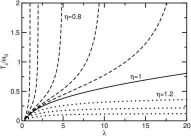
Figure 1: Critical temperature as function of the pairing coupling $\lambda$ for different values of $\eta$. Dashed lines: $\eta<1$; dotted lines: $\eta>1$; the solid line is the conventional Eliashberg result for $\eta=1$. From upper to lower line: $\eta=0,0.5,0.8,0.9,0.95,1,1.2,1.5,2$.

We would like to point out that the analytical divergence $T_{c}\rightarrow\infty$ for $\lambda\rightarrow\lambda_{c}$ is strictly related to the infinite bandwidth model employed in Eqs. (1)-(2). On the other hand, in physical systems the presence of a finite bandwidth $W$ determines an additional regime, $T_{c}\gg W$, where the analytical divergence of $T_{c}$ at $\lambda_{c}$ is removed and $T_{c}\propto\lambda W$ (Appendix A). In this respect the bandwidth $W$ defines an upper limiting regime for $T_{c}$. Since in physical systems, however, $W$ is some orders of magnitude bigger than the bosonic energy scale $\omega_{0}$, in the following, for sake of simplicity, we shall concentrate on the infinite bandwidth limit $W\gg T_{c},\Delta,\omega_{0}$, keeping in mind however that the analytical divergences found in this case will be removed when finite bandwidth effects are included in the regime $T_{c}\gtrsim W$.

In Fig. 1 we show the critical temperature $T_{c}$ as function of the electron-boson interaction $\lambda$ obtained from the numerical solution of Eqs. (1)-(2). We see that the conventional Eliashberg case $\eta=1$, where $T_{c}$ scales as $\sqrt{\lambda}$, represents rather an exception than the rule: for $\eta<1$ $T_{c}$ diverges at finite values of $\lambda$ determining, for each $\eta$, a upper value of $\lambda$ above which the system is superconducting at any temperature, while, for $\eta>1$, $T_{c}$ saturates for $\lambda\rightarrow\infty$ at some value which also is dependent on $\eta$. We can estimate in this case (see Appendix A) an upper limit for $T_{c}$:

$$T_{c,\rm max}^{\eta>1} = \frac{\omega_{0}}{2\pi\sqrt{\eta-1}}.$$ (6)

Before to proceed on, we would briefly comment on the $T_{c}$ divergence at finite $\lambda$ for $\eta<1$. This result seems to contradict apparently the BCS scenario $T_{c}\propto\exp(-1/\lambda)$ which can be thought as the extremely unbalanced $\eta=0$ case where the one-particle renormalization processes are disregarded. However, a closer look at Eq. (3) shows that a fundamental role in deriving Eqs. (4)-(5) is played by the proper treatment of the retarded nature of the electron-boson interaction, which gives rise to the correlation between $\omega_{n}$ and $\omega_{m}$ within the energy window $\omega_{0}$. In this sense, neglecting the $Z$-function for $\eta=0$ in Eqs. (1)-(2) corresponds to a “retarded BCS” theory. This is quite different from the usual conventional BCS framework where the interaction is supposed to be non-retarded and the frequencies $\omega_{n}$ and $\omega_{m}$ are uncorrelated. This scenario can be achieved in the retarded BCS context only in the limit $\omega_{0}\rightarrow\infty$, which enforces the $T_{c}/\omega_{0}\rightarrow 0$ limit, namely, the weak-coupling regime.

III Superconducting gap $\Delta_{\rm M}$ vs. $\lambda$

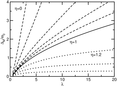
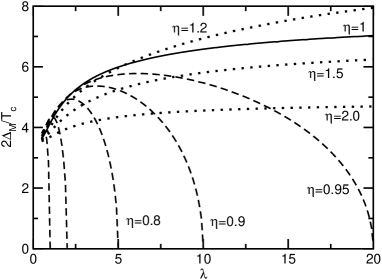
Figure 2: Matsubara superconducting gap $\Delta_{\rm M}$ (upper panel) and ratio $2\Delta_{\rm M}/T_{c}$ (lower panel) as function of the pairing coupling $\lambda$ for the same values of $\eta$ as in Fig. 1

Interesting enough, the $\Delta$ vs. $\lambda$ behavior in an unbalanced superconductor can be quite different from the $T_{c}$ vs. $\lambda$. In Fig. 2 we plot the Matsubara superconducting gap $\Delta_{\rm M}$, defined as $\Delta_{\rm M}=\lim_{T\rightarrow 0}\Delta_{n=0}$, and the ratio $2\Delta_{\rm M}/T_{c}$ as function of the electron-boson coupling $\lambda$. We remind that, although $\Delta_{\rm M}$ underestimates the physical gap edge obtained by the analytical continuation on the real axis, the analytical dependence of these two quantities is usually the same, so that $\Delta_{\rm M}$ can be reasonable employed to study the limiting behavior of the superconducting gap in the strong-coupling regime. Detailed investigations on the real axis are however needed to assess in a more formal way this issue. Fig. 2 shows that, while for $\eta>1$ $\Delta_{\rm M}$ has a saturating behavior similar as $T_{c}$, in the case $\eta<1$ the superconducting gap does not diverge at some finite value of $\lambda$, as $T_{c}$, but rather increases linearly with the electron-boson coupling. This different behavior can be also understood by applying some analytical derivations properly generalized for unbalanced superconductors.cmm Assuming $\Delta_{\rm M}\gg\omega_{0}$, and following Eqs. (4.29)-(4.35) of Ref. carbotte_rmp, , the superconducting gap $\Delta_{\rm M}$ is determined by the following relation:

$$1+\eta\lambda\frac{\pi\omega_{0}}{2\Delta_{\rm M}}-c_{1}\eta\lambda\frac{\omega_{0}^{2}}{\Delta_{\rm M}^{2}} = \lambda\frac{\pi\omega_{0}}{2\Delta_{\rm M}}-c_{2}\lambda\frac{\omega_{0}^{2}}{\Delta_{\rm M}^{2}},$$ (7)

where $c_{1}$, $c_{2}$ are constant factors whose value is discussed in Appendix A. For $\eta=1$ the terms $\propto\omega_{0}/\Delta_{\rm M}$ on both the left and right sides cancel out, so that $\Delta_{\rm M}\propto\sqrt{\lambda}\omega_{0}$.cmm ; carbotte_rmp This is no longer true for $\eta\neq 1$. In particular, for $\eta<1$ we find

$$\Delta_{\rm M} = \lambda(1-\eta)\frac{\pi\omega_{0}}{2},$$ (8)

while, for $\eta>1$, Eq. (7) does not admit solution signalizing, once more, that the initial assumption $\Delta_{\rm M}\gg\omega_{0}$ is inconsistent in this limit and that $\Delta_{\rm M}$ must be saturate for $\lambda\rightarrow\infty$. By taking into account higher order terms we found an upper limit $\Delta_{\rm M}$ for $\eta>1$ in the regime $\lambda\rightarrow\infty$ in similar way as done for $T_{c}$:

$$\Delta_{\rm M,max} = \frac{4(\eta c_{1}-c_{2})\omega_{0}}{2\pi(\eta-1)}.$$ (9)

Note that $\Delta_{\rm M,max}$ in Eq. (9) diverges as $1/(\eta-1)$ whereas $T_{c,{\rm max}}$ in Eq. (6) scales as $T_{c,{\rm max}}\sim 1/\sqrt{\eta-1}$. This means that the ratio $2\Delta_{\rm M}/T_{c}$ is not bounded for $\eta>1$ and it can be even larger than in the Eliashberg case $\eta=1$ and formally diverging for $\eta\rightarrow 1$, in agreement with the numerical results shown in Fig. 2.

IV Temperature dependence of $\Delta_{\rm M}(T)$

In the previous sections we have studied the strong coupling behaviors of the critical temperature $T_{c}$ and of the zero temperature Matsubara gap $\Delta_{\rm M}$ in the limit $\lambda\gg 1$. We have seen for instance that, in the $\eta<1$ case, $T_{c}$ diverges at some critical value $\lambda_{c}$, so that for $\lambda>\lambda_{c}$ the system is superconducting at any temperature. This behavior is in contrast with the one of the Matsubara gap $\Delta_{\rm M}$ which is always finite for any $\lambda$ and scales linearly with $\lambda$ for $\eta<1$. As shown in Fig. 2, these different behaviors are reflected in a ratio $2\Delta_{\rm M}/T_{c}$ smaller than the BCS limit 3.53 and vanishing for $\lambda\rightarrow\lambda_{c}$. In this situation an interesting issue to investigate is the temperature dependence of the superconducting gap $\Delta(T)$, which is reflected in a number of observable physical behaviors, as the temperature profile of the magnetic field $H_{c}(T)$, of the London penetration depth $\lambda_{\rm L}(T)$ or of the specific heat $C_{V}(T)$. Also intriguing is the situation $\eta<1$ and $\lambda>\lambda_{c}$, where a finite superconducting gap exists at zero temperature but where no finite critical temperature is predicted. In this case the temperature behavior of the gap itself is not clear and needs to be investigated.

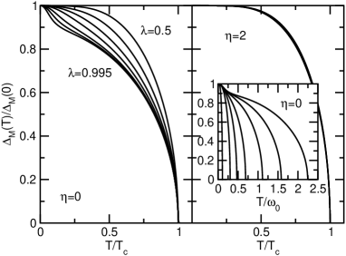
Figure 3: Temperature evolution of the Matsubara superconducting gap $\Delta_{\rm M}(T)/\Delta_{\rm M}(0)$ for different unbalanced cases. Left panel: $\eta=0$ ($\lambda_{c}=1$) and different coupling (from top to bottom) $\lambda=0.5,0.8,0.9,0.95,0.98,0.99,0.995$. Right panel: $\eta=2$ and (from bottom to top, but barely distinguishable) $\lambda=5,10,20$. Inset: same quantities as in the left panel ($\eta=0$) but as function of $T/\omega_{0}$.

In Fig. 3 we show the temperature dependence of $\Delta_{\rm M}(T)/\Delta_{\rm M}(0)$ (defined as $\Delta_{\rm M}(T)=\Delta_{n=0}$) for different characteristic cases, namely for $\eta=0$ and different $\lambda<\lambda_{c}$, and for $\eta=2$ and different $\lambda\gtrsim 1$. Most regular is the $\Delta_{\rm M}(T)$ vs. $T$ dependence for $\eta>1$, where $\Delta_{\rm M}(T)$ follows a conventional behavior, independently of the coupling $\lambda$. This regular behavior can be understood by reminding that for $\eta>1$, even for very large coupling $\lambda$, the values of $T_{c}$ and of the superconducting gap $\Delta_{\rm M}(T)$ are always finite and (at most) of the same order of the energy $\omega_{0}$. Quite different is the case of $\eta<1$, here represented by $\eta=0$, where $\Delta_{\rm M}(T)$ shows a temperature dependence remarkably different from the BCS one. For $\lambda$ close to $\lambda_{c}$, in particular, the superconducting Matsubara gap has a first initial drop followed by a more regular dependence. This change of curvature represents the crossover between a small temperature ($T/\omega_{0}\lesssim 1/4$) to a large temperature ($T/\omega_{0}\gtrsim 1/4$) regime, as shown in the inset of Fig. 3 where we plot $\Delta_{\rm M}(T)/\Delta_{\rm M}(0)$ as function of $T/\omega_{0}$. Note that, while the value of the critical temperature $T_{c}$ is strongly dependent on the coupling $\lambda$, the initial dependence of $\Delta_{\rm M}(T)$ is only weakly dependent on $\lambda$. We remind indeed that the $T_{c}$ divergence for $\lambda\rightarrow\lambda_{c}$ is essentially a by-product of having reached the $T/\omega_{0}\gg 1$ for a finite $\lambda$ in the unbalanced case. We can thus understand the results of Fig. 3 in the following way: for low temperature ($T/\omega_{0}\lesssim 1/4$) the superconducting gap probes a pairing kernel which is actually increased by the lack of unbalance, but still regular, (remind that $\Delta_{\rm M}(T=0)$, contrary to $T_{c}$, does not diverge at $\lambda_{c}$, but it steadily increases as $\propto\lambda$ in the strong-coupling regime). For low temperature $\Delta_{\rm M}(T)/\Delta_{\rm M}(0)$ follows thus a standard-like behavior which would close to some finite $T^{\prime}_{c}$ not diverging at $\lambda_{c}$. When $\lambda$ is however close enough to $\lambda_{c}$, the range $T/\omega_{0}\gtrsim 1/4$ is achieved before $T^{\prime}_{c}$ is actually reached; in this regime high temperature effects become dominant in the pairing kernel, reflected in a change of the $\Delta_{\rm M}(T)$ vs. $T$ trend and in a final, physical, $T_{c}$ which diverges at $\lambda\rightarrow\lambda_{c}$.

It is interesting to investigate also how the superconducting gap $\Delta_{\rm M}(T)$ closes at $T_{c}$. In the conventional, perfectly balanced, Eliashberg theory the normalized gap $\Delta(T)/\pi T_{c}$ (or equivalently $\Delta(T)/\Delta(T=0)$) scales indeed for $T\rightarrow T_{c}$ as $(\Delta(T)/\pi T_{c})^{2}\sim c\delta$, where $\delta=1-T/T_{c}$ and where $c$ is a finite constant which, in the weak-coupling BCS limit $\lambda\ll 1$, is $c=0.95$ whereas for $\lambda\gg 1$ one gets $c=2$. This scenario is qualitatively different in the case of unbalanced $\eta<1$ superconductors (Fig. 3, left panel) where the constant $c$ strongly depends on the coupling $\lambda$.

For $\eta<1$ a first insight about the temperature dependence of $\Delta_{\rm M}(T)$ close at $T_{c}$ is gained simply by considering that, for $\lambda\rightarrow\lambda_{c}$, $\Delta_{\rm M}(0)$ is finite while $T_{c}\rightarrow\infty$, with a ratio $2\Delta_{\rm M}(0)/T_{c}\rightarrow 0$. This means that, as $\lambda\rightarrow\lambda_{c}$, the constant $c$ must vanish. This result can be shown in a more quantitative way (see Appendix A) by employing a one-Matsubara-gap approximationcarbotte_rmp which, for $T\simeq T_{c}$ and for $T_{c}\gg\omega_{0}$, is quite reasonably justified. For generic $\eta$ one obtains thus

$$\frac{\Delta_{0}^{2}}{\pi^{2}T_{c}^{2}} = 4\delta\frac{1-\lambda(1-\eta)}{2-\lambda(1-\eta)},$$ (10)

where $\delta=1-T/T_{c}$. Note that Eq. (10) reduces to the standard relation $(\Delta_{0}/\pi T_{c})^{2}=2\delta$ for $\eta=1$.carbotte_rmp On the other hand, for $\eta<1$

$$\frac{\Delta_{0}^{2}}{\pi^{2}T_{c}^{2}} = 4\delta\frac{\lambda_{c}-\lambda}{2\lambda_{c}-\lambda},$$ (11)

showing that the coefficient $c$ vanishes as $c\propto\lambda_{c}-\lambda$ for $\lambda\rightarrow\lambda_{c}$.

V Other thermodynamical quantities

The anomalous temperature dependence of $\Delta_{\rm M}(T)$ is reflected also in other thermodynamical, measurable quantities, as the specific heat $C_{V}(T)$ or the magnetic critical field $H_{c}(T)$. In order to investigate these properties we evaluate numerically the free energy difference $\Delta F$ between the superconducting and the normal state,carbotte_rmp

$$\Delta F(T) = -\pi TN(0)\sum_{n}\left(Z^{\rm S}_{n}-\frac{Z^{\rm N}_{n}|\omega_{n}|}{\sqrt{\omega_{n}^{2}+\Delta_{n}^{2}}}\right)$$ (12)

$$\times\left(\sqrt{\omega_{n}^{2}+\Delta_{n}^{2}}-|\omega_{n}|\right),$$

where $N(0)$ is the electron density of states at the Fermi level and $Z^{\rm S}_{n}$, $Z^{\rm N}_{n}$ are the $Z$-renormalization functions calculated respectively in the superconducting and in the normal state. From Eq. (12) we obtain the magnetic critical field $H_{c}(T)=\sqrt{-8\pi\Delta F(T)}$ and the specific heat difference as $\Delta C_{V}(T)=-T\partial^{2}\Delta F/\partial T^{2}$. One can also obtain the total specific heat $C_{V}(T)=\Delta C_{V}(T)+C_{V}^{\rm N}$ by adding the contribution that the system would have in the normal state, $C_{V}^{\rm N}=\gamma T$, where $\gamma=(2/3)\pi^{2}N(0)(1+\eta\lambda)$ is the Sommerfeld constant. In similar way we can evaluate the London penetration depth $\lambda_{\rm L}(T)$ as:carbotte_rmp

$$\frac{1}{e^{2}v_{\rm F}^{2}N(0)\lambda_{\rm L}^{2}(T)} = \frac{2\pi T}{3}\sum_{n}\frac{\Delta_{n}^{2}}{Z_{n}\left[\omega_{n}^{2}+\Delta_{n}^{2}\right]^{3/2}},$$ (13)

where $e$ is the electron charge and $v_{\rm F}$ the Fermi velocity.

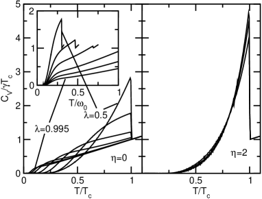
Figure 4: Specific heat $C_{V}(T)$ for the two characteristic unbalanced cases previous considered. Left panel: $\eta=0$ ($\lambda_{c}=1$) and $\lambda=0.5,0.8,0.9,0.95,0.98,0.99,0.995$. Right panel: $\eta=2$ and $\lambda=5,10,20$. Inset: specific heat for $\eta=0$ as function of $T/\omega_{0}$.

In Fig. 4 we show the temperature dependence of the specific heat as function of $\lambda$ for the two representative cases $\eta=0$, $\eta=2$. In this latter case the specific heat has a regular activated behavior and it is almost independent of $\lambda$, in agreement with the corresponding weakly $\lambda$ dependence of the temperature behavior of $\Delta_{\rm M}(T)$ reported in Fig. 3. Note also that for this value of $\eta$ the asymptotic value $\lambda\rightarrow\infty$ of the specific heat jump $\Delta C_{V}/\gamma T_{c}\simeq 4.2$, is quite larger than the BCS limit, $(\Delta C_{V}/\gamma T_{c})_{\rm BCS}\simeq 1.43$, pointing out that the superconductors is in an effective strong-coupling limit. We should remark that the asymptotic value $\lim_{\lambda\rightarrow\infty}\Delta C_{V}/\gamma T_{c}$ is actually dependent on the specific value of the parameter $\eta>1$.

Quite anomalous is also the temperature behavior for $\eta<1$. In this case we see that approaching $\lambda\rightarrow\lambda_{c}$ the jump is remarkably reduced. Eqs. (10)-(11) can be used to estimate the jump $\Delta C_{V}$ at $T_{c}$ of the specific heat. Using once more the one-Matsubara gap approximation, and employing a standard analysis,carbotte_rmp one can show that the formal expression for the free energy difference $\Delta F$ close to $T_{c}$ is just equal as in the standard case,

$$\Delta F=-\frac{N(0)(\pi T_{c})^{2}}{2}\left(1+\eta\lambda\frac{\omega_{0}^{2}}{4\pi^{2}T^{2}}\right)\left(\frac{\Delta_{0}(T)}{\pi T_{c}}\right)^{4}.$$ (14)

Plugging Eq. (10) and (5) in (14), and using the standard derivation of $\Delta C_{V}$, we obtain thus

$$\frac{\Delta C_{V}}{\gamma T_{c}} = \frac{24}{1+\eta\lambda}\left(1+\eta\frac{\lambda_{c}-\lambda}{\lambda_{c}}\right)\left(\frac{\lambda_{c}-\lambda}{2\lambda_{c}-\lambda}\right)^{2},$$ (15)

showing that, for $\eta<1$, also $\Delta C_{V}/\gamma T_{c}$ as $(\Delta_{0}/\pi T_{c})^{2}$ scales as $\propto\lambda_{c}-\lambda$ for $\lambda\rightarrow\lambda_{c}$. Once more, Eq. (15) reduces to the standard analytical result $\Delta C_{V}/\gamma T_{c}=12/\lambda$ for $\eta=1$ and $\lambda\rightarrow\infty$.mwc It is interesting to note that the vanishing of $\Delta C_{V}/\gamma T_{c}$ for $\lambda\rightarrow\lambda_{c}$ is mainly due to the vanishing of $\Delta C_{V}\propto(\lambda_{c}-\lambda)^{3/2}$, whereas $T_{c}\propto 1/\sqrt{\lambda_{c}-\lambda}$. This means that, contrary to the perfectly balanced case $\eta=1$ where the vanishing of $\Delta C_{V}/\gamma T_{c}$ is driven by $\gamma T_{c}\rightarrow\infty$ which overcomes the divergence of $\Delta C_{V}$, in the unbalanced $\eta<1$ case the specific heat jump $\Delta C_{V}$ is itself vanishing. Such observation points out that, although $T_{c}$ is much higher, the superconducting properties in the $T/\omega_{0}$ regime of $\eta<1$ unbalanced superconductors are much weaker than the usual.

This scenario is once more outlined in Fig. 4, where we see that the vanishing of $\Delta C_{V}$ is accompanied by the developing of a shoulder at $T\approx\omega_{0}/4$ (see inset). Above this temperature the specific heat scales roughly linearly with $T$ as a normal ungapped metal with a smaller and smaller jump at $T_{c}$ as $\lambda\rightarrow\lambda_{c}$.

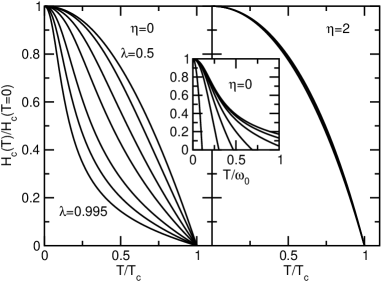
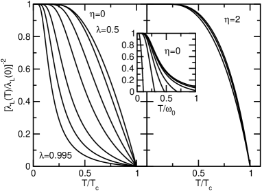
Figure 5: Temperature dependence of the magnetic critical field $H_{c}(T)/H_{c}(0)$ and of the London penetration depth $\lambda_{\rm L}^{2}(0)/\lambda_{\rm L}^{2}(T)$ for the two characteristic unbalanced cases previous considered. Left panels: $\eta=0$ ($\lambda_{c}=1$) and $\lambda=0.5,0.8,0.9,0.95,0.98,0.99,0.995$. Right panels: $\eta=2$ and $\lambda=5,10,20$. Insets: the same quantities as function of $T/\omega_{0}$.

A similar trend is observed in the study of the temperature dependence of the magnetic critical field $H_{c}$ and of the London penetration depth $\lambda_{\rm L}$, shown in Fig. 5. For $\eta=2$ we find again that the temperature dependence of both $H_{c}(T)$ and $\lambda_{\rm L}^{-2}(T)$ presents again a conventional behavior with even a more marked curvature with respect to the BCS curve. This is compatible with the specific heat jump which is also larger than the BCS limit. Quite different is the case for $\eta=0$. Here we observe a change of curvature at low temperature which is more marked as $\lambda\rightarrow\lambda_{c}$.note-hc Once again such change of curvature occurs for $T\gtrsim\omega_{0}/4$ and for $\lambda\simeq\lambda_{c}$ it is reflected in a sudden drop of $H_{c}(T)$ and $\lambda_{\rm L}^{-2}(T)$ signalling once more that, although the critical temperature is strongly increasing, the high temperature superconducting properties of unbalanced systems are quite poor.

VI Summary and discussion

In this paper we have investigated the properties of “unbalanced” retarded superconductors, namely systems where the electron-boson coupling $\lambda_{Z}$ in the one-particle renormalization function is different than the one relevant for the gap equation, $\lambda_{\Delta}$. We have shown that the superconducting properties are strongly dependent on the ratio $\eta=\lambda_{Z}/\lambda_{\Delta}$. We have analyzed both the cases $\eta>1$ and $\eta<1$. In the first case we show that, contrary to the perfectly balanced case, the critical temperature is always finite and it even saturates at a finite value for $\lambda\rightarrow\infty$. The superconducting properties in this case are quite similar to the conventional case in the weak-intermediate regime where the magnitude of $\eta$ rules the relevance of the strong-coupling effects. Quite anomalous is on the other hand the case $\eta<1$, which is relevant in a variety of situations as for instance for $d$-wave superconductors. In this case we find that the critical temperature, in the infinite bandwidth limit, diverges at a finite value $\lambda_{c}\approx 1$ ($\lambda_{c}=1$ for $\eta=0$). We show also that, although for $\lambda>\lambda_{c}$ the critical temperature $T_{c}$ is strongly enhanced for $\lambda\rightarrow\lambda_{c}$, the zero temperature gap is still finite and it scales as $\Delta\propto\lambda$. The anomalous temperature dependence of the superconducting gap is reflected in a variety of other physical properties, as the magnetic critical field, the penetration depth and the specific heat. All these quantities show a strong anomaly at $T\gtrsim\omega_{0}/4$ above which the system presents very weak superconducting properties, which however persist up to the higher critical temperature $T_{c}$. We would like to remark once more that in real systems finite bandwidth effects remove the analytical divergence of $T_{c}$ at $\lambda_{c}$ when $T_{c}\gg W$.

These results suggest an interesting pseudogap scenario. In the $T_{c}^{\prime}\lesssim T\lesssim T_{c}$ regime indeed, since the superconducting binding energies are quite small, the robustness of the long-range order of this phase towards phase fluctuations, disorder, phase separation and other different kinds of instability is highly questionable. In case of loss of the long-range order, these weak superconducting properties will present themselves as a pseudogap phase in the range temperature $T_{c}^{\prime}\lesssim T\lesssim T_{c}$, where the temperature $T_{c}^{\prime}$ will appear as the thermodynamical critical temperature where true lost range order is lost, and $T_{c}\approx T_{c}$ will set the pseudogap temperature $T^{*}$. Note that, even in this case, the critical temperature of the long-range order will result $T_{c}^{\prime}\approx\omega_{0}/4$, which can be significantly higher than the predictions of the standard Eliashberg’s theory.

Before concluding, we would like to spend some more words about the physical meaning of the $T_{c}$ divergence for $\eta<1$. On the mathematical ground, we have seen that, contrary to the conventional balanced case, in unbalanced superconductors the Cooper instability is driven by the $n=m$ term in Eq. (3). In physical terms this corresponds to consider the classical limit $T\gg\omega_{0}$ of the bosons. This is quite different from the usual Eliashberg’s theory where only virtual bosons, which a characteristic energy scale $\omega_{0}$, are responsible of the pairing. Just as for the linear behavior $\rho(T)\propto\lambda T$ of the resistivity, in the classical limit $T\gg\omega_{0}$ the energy scale $\omega_{0}$ does not provide anymore any upper limit and the effective pairing is mainly ruled by the increasing bosonic population $n(T)\propto T$ with temperature. In the absence of any other competing effect, increasing temperature will result thus in a stronger pairing with a positive feedback which would lead a high critical temperature $T_{c}\gg\omega_{0}$, and the only limiting energy scale in this case is provided by the electronic bandwidth. In this scenario a competing effect in balanced superconductor is provided by the fact that the increase of the boson population, as $T$ increases, would act in a similar way in the self-energy channel. The competition between these two effects give rise to the well-known $T_{c}\sqrt{\lambda}\omega_{0}$ dependence in perfectly balanced superconductors with $\eta=1$ Such equilibrium does not occur however in unbalanced superconductors with $\eta<1$ where the gain in the Cooper channel is larger than the loss in the self-energy. In this case, at sufficiently large $T$, the increase of the Cooper pairing due to the boson population will prevail over the one-particle renormalization effects and a superconducting ordering can be sustained up to high temperatures $T_{c}$ limited only by the electronic bandwidth energy scale.

Appendix A Analytical formulas for asymptotic behaviors $T_{c}\gg\omega_{0}$, $\Delta_{\rm M}\gg\omega_{0}$

In this appendix we derive some useful limit expressions for the critical temperature $T_{c}$ and the Matsubara superconducting gap $\Delta_{\rm M}$ in the regimes $T_{c}\gg\omega_{0}$, $\Delta_{\rm M}\gg\omega_{0}$.

A.1 Critical temperature $T_{c}$

Let us start by considering Eq. (3) and let us assume $T_{c}\gg\omega_{0}$. In this regime we can employ the one-Matsubara-gap approximation,carbotte_rmp where the only not vanishing terms of the Matsubara gap function $\Delta_{n}$ are $\Delta_{n=0}=\Delta_{n=-1}$. We have thus:

$$\Delta_{0} = \lambda\Delta_{0}+\lambda\Delta_{-1}\frac{\omega_{0}^{2}}{4\pi^{2}T_{c}^{2}}$$ (16)

$$-\lambda\eta\Delta_{0}\sum_{m}\frac{\omega_{0}^{2}}{\omega_{0}^{2}+(\omega_{n}-\omega_{m})^{2}}\mbox{sgn}[\omega_{m}],$$

and, reminding that $\Delta_{-1}=\Delta_{0}$ and $\sum_{m}\mbox{sgn}[\omega_{m}]\omega_{0}^{2}/[\omega_{0}^{2}-(\omega_{n=0}-\omega_{m})]=1$, we have

$$1=\lambda(1-\eta)+\lambda\frac{\omega_{0}^{2}}{4\pi^{2}T_{c}^{2}}.$$ (17)

For $\eta=1$ the first term on the right hand side is zero, and we recover the usual result $T_{c}^{\eta=1}=\sqrt{\lambda}\omega_{0}/(2\pi)$. On the other hand, for $\eta<1$ we obtain

$$T_{c}^{\eta<1} = \frac{\omega_{0}}{2\pi}\sqrt{\frac{\lambda}{1-\lambda(1-\eta)}},$$ (18)

or, equivalently,

$$T_{c}^{\eta<1} = \frac{\omega_{0}}{2\pi}\sqrt{\frac{\lambda_{c}\lambda}{\lambda_{c}-\lambda}},$$ (19)

where $\lambda_{c}=1/(1-\eta)$.

Finally, The same expression (18) can be used to evaluated an upper limit for $T_{c}$ in the case $\eta>1$. We can write thus

$$T_{c}^{\eta>1} = \frac{\omega_{0}}{2\pi}\sqrt{\frac{\lambda}{1+\lambda(\eta-1)}},$$ (20)

and, for $\lambda\rightarrow\infty$,

$$T_{c,{\rm max}}^{\eta>1} = \frac{\omega_{0}}{2\pi\sqrt{\eta-1}}.$$ (21)

Note that Eq. (21) predicts a saturating upper limit for $T_{c}^{\eta>1}$ for $\lambda\rightarrow\infty$, violating the assumption $T_{c}\gg\omega_{0}$. This value, $T_{c,{\rm max}}^{\eta>1}$, can be thus assumed as a upper limit for the asymptotic behavior of $T_{c}^{\eta>1}$ in the regime $\lambda\rightarrow\infty$.

Let us now consider finite bandwidth effects in the $\eta<1$ case. For simplicity we shall focus on the representative case $\eta=0$. Finite bandwidth effects can be included in the linearized Eliasberg’s equations, (3), by replacing the term $\pi/|\omega_{m}|\rightarrow(2/\omega_{m})\arctan(W/2\omega_{m})$, where $W/2$ is the half-bandwidth in a symmetric particle-hole system. In this case, in order to obtain an analytical expression for $T_{c}$ in the limit $T_{c}\gg\omega_{0}$, it is sufficient to retain only the $n=m$ term in Eq. (3), and, in the one-Matsubara-gap approximation, we obtain

$$\Delta_{0}=\lambda\Delta_{0}\frac{2}{\pi}\arctan\left(\frac{W}{2\pi T_{c}}\right).$$ (22)

Inverting Eq. (22) we obtain thus, for $T_{c}\gg W$, $T_{c}=(W/2\pi)/\tan(\pi/2\lambda)\approx\lambda W/\pi^{2}$, showing that Eq. (19) is valid as far as $\omega_{0}\ll T_{c}\ll W$, whereas for $T_{c}\gg W$ the divergence at $\lambda_{c}$ is removed and a linear behavior as function of $\lambda$ is achieved.

A.2 Superconducting Matsubara gap $\Delta_{\rm M}$

Let us now investigate the asymptotic behavior of the zero temperature Matsubara gap $\Delta_{\rm M}$. Once more, we assume the limit $\Delta_{\rm M}\gg\omega_{0}$ and we shall check later the consistency of this ansatz. To get an analytical expression for $\Delta_{\rm M}$, we essentially follow Refs. carbotte_rmp, ; cmm, . Transforming, in the zero temperature limit, the Matsubara sum in an integral, $T\sum_{m}\rightarrow\int d\omega/2\pi$, we can write:

$$Z(\omega) = 1+\frac{\lambda\eta}{2\omega}\int\frac{d\omega^{\prime}\omega^{\prime}}{\sqrt{\omega^{\prime 2}+\Delta^{2}(\omega^{\prime})}}\frac{\omega_{0}^{2}}{\omega_{0}^{2}+(\omega-\omega^{\prime})^{2}},$$ (23)

$$Z(\omega)\Delta(\omega) = \frac{\lambda}{2}\int\frac{d\omega^{\prime}\Delta(\omega^{\prime})}{\sqrt{\omega^{\prime 2}+\Delta^{2}(\omega^{\prime})}}\frac{\omega_{0}^{2}}{\omega_{0}^{2}+(\omega-\omega^{\prime})^{2}}.$$ (24)

We also employ the simple model:carbotte_rmp ; cmm

$$\Delta(\omega)=\left\{\begin{array}[]{ll}\Delta_{\rm M}&\hskip 14.22636pt\mbox{for $\omega<\alpha\Delta_{\rm M}$},\\ 0&\hskip 14.22636pt\mbox{for $\omega>\alpha\Delta_{\rm M}$},\end{array}\right.$$ (25)

which we have tested numerically to be appropriate even for unbalanced superconductors. Here $\alpha$ is a constant of the order of unity. Using this model and expanding Eqs. (23)-(24) in powers of $\omega_{0}/\Delta_{\rm M}$ we end up with:

$$1+\eta\lambda\frac{\pi\omega_{0}}{2\Delta_{\rm M}}-c_{1}\eta\lambda\frac{\omega_{0}^{2}}{\Delta_{\rm M}^{2}} = \lambda\frac{\pi\omega_{0}}{2\Delta_{\rm M}}-c_{2}\lambda\frac{\omega_{0}^{2}}{\Delta_{\rm M}^{2}},$$ (26)

where $c_{1}$, $c_{2}$ are constant factors depending on $\alpha$. For $\alpha=1$ we have for instance $c_{1}=2(\sqrt{2}-1/2)$, $c_{2}=\sqrt{2}$,cmm while for $\alpha=2$ we have $c_{1}=\sqrt{5}-1$, $c_{2}=\sqrt{5}/2$.carbotte_rmp

In the perfectly balanced case $\eta=1$ the linear terms in $\omega_{0}/\Delta_{\rm M}$ in Eq. (26) cancel out, and one recovers the usual result $\Delta_{\rm M}^{\eta=1}=\sqrt{\lambda}\sqrt{c_{1}-c_{2}}\omega_{0}$ (we remind that $c_{1}-c_{2}$ is a positive quantity). On the other hand, for $\eta<1$ the solution of Eq. (26) is dominated by the linear terms giving:

$$\Delta_{\rm M}^{\eta<1} = \lambda(1-\eta)\frac{\pi\omega_{0}}{2}.$$ (27)

More complex is the case $\eta>1$, where retaining only the linear term is not sufficient. In this case one needs to consider explicitly also the $(\omega_{0}/\Delta_{\rm M})^{2}$ and to solve the quadratic equation (26). We obtain:

$$\left(\frac{\Delta_{\rm M}}{\omega_{0}}\right)^{2}+\frac{\lambda\pi(\eta-1)}{2}\left(\frac{\Delta_{\rm M}}{\omega_{0}}\right)-\lambda(\eta c_{1}-c_{2})=0,$$ (28)

so that

$$\frac{\Delta_{\rm M,max}^{\eta>1}}{\omega_{0}} = \frac{1}{2}\left[-\frac{\lambda\pi(\eta-1)}{2}\right.$$ (29)

$$\left.+\sqrt{\frac{\lambda^{2}\pi^{2}(\eta-1)^{2}}{4}+4\lambda(\eta c_{1}-c_{2})}\right]$$

$$\simeq \frac{4(\eta c_{1}-c_{2})}{2\pi(\eta-1)},$$

showing that for $\eta>1$ $\Delta_{\rm M}$ saturates at a finite value for $\lambda\rightarrow\infty$, and Eq. (29) can be considered an upper limit for it.

A.3 Temperature dependence of $\Delta_{\rm M}(T)$

In this section we investigate the temperature behavior of the Matsubara gap $\Delta_{\rm M}(T)$ close to $T_{c}$. We assume once more th limit $T_{c}\gg\omega_{0}$ and thus the validity of the one-Matsubara-gap model. Within these approximation we can rewrite Eqs. (1) as:

$$Z_{0} = 1+\eta\lambda\sum_{m=0,-1}\frac{\omega_{0}^{2}}{\omega_{0}^{2}+(\omega_{n}-\omega_{m})^{2}}\frac{\omega_{m}}{\sqrt{\omega_{m}^{2}+\Delta_{m}^{2}}}$$ (30)

$$+\sum_{m\neq 0,-1}\frac{\omega_{0}^{2}}{\omega_{0}^{2}+(\omega_{n}-\omega_{m})^{2}}\mbox{sgn}[\omega_{m}]$$

$$= 1+\frac{\eta\lambda\pi T}{\sqrt{\pi^{2}T^{2}+\Delta_{0}^{2}}}\left(1-\frac{\omega_{0}^{2}}{4\pi^{2}T^{2}}\right)+\frac{\eta\lambda\omega_{0}^{2}}{4\pi^{2}T^{2}},$$

where we have used $\Delta_{0}=\Delta_{-1}$, and in similar way,

$$Z_{0}\Delta_{0} = \lambda\pi T\frac{\Delta_{0}}{\sqrt{\pi^{2}T^{2}+\Delta_{0}^{2}}}\left(1+\frac{\omega_{0}^{2}}{4\pi^{2}T^{2}}\right).$$ (31)

Plugging (30) in (31) we have:

$$\Delta_{0} = \lambda(1-\eta)\frac{\pi T\Delta_{0}}{\sqrt{\pi^{2}T^{2}+\Delta_{0}^{2}}}$$ (32)

$$+\lambda(1+\eta)\frac{\pi T\Delta_{0}}{\sqrt{\pi^{2}T^{2}+\Delta_{0}^{2}}}\frac{\omega_{0}^{2}}{4\pi^{2}T^{2}}-\frac{\eta\lambda\omega_{0}^{2}\Delta_{0}}{4\pi^{2}T^{2}},$$

which we can rewrite as:

$$\frac{\sqrt{\pi^{2}T^{2}+\Delta_{0}^{2}}}{\pi T} = \frac{\lambda(1-\eta)+\lambda(1+\eta)\frac{\displaystyle\omega_{0}^{2}}{\displaystyle 4\pi^{2}T^{2}}}{\left(1+\frac{\displaystyle\eta\lambda\omega_{0}^{2}}{\displaystyle 4\pi^{2}T^{2}}\right)}.$$ (33)

Expanding left- and right-hand sides of Eq. (33) at the second order in $\Delta$ and at the linear order of $\delta=1-T/T_{c}$, we have:

$$\frac{\Delta_{0}^{2}}{2\pi^{2}T_{c}^{2}} = \frac{2\delta\lambda\omega_{0}^{2}}{4\pi^{2}T_{c}^{2}+\eta\lambda\omega_{0}^{2}}$$ (34)

$$= 2\delta\frac{1-\lambda(1-\eta)}{2-\lambda(1-\eta)},$$

where we made use of Eq. (17). Eq. (34) reduces to the standard relation $(\Delta_{0}/\pi T_{c})^{2}=2\delta$ in the perfectly balanced case $\eta=1$.carbotte_rmp On the other hand, for $\eta<1$ we have

$$\frac{\Delta_{0}^{2}}{\pi^{2}T_{c}^{2}} = 4\delta\frac{\lambda_{c}-\lambda}{2\lambda_{c}-\lambda},$$ (35)

which shows that $\Delta(T)\simeq c\sqrt{T_{c}-T}$ (for $T\simeq T_{c}$) with a vanishing coefficient $c$ for $\lambda\rightarrow\lambda_{c}$. Finally, for $\eta>1$, Eq. (34) is well-behaved in the limit $\lambda\rightarrow\infty$ and it gives

$$\frac{\Delta_{0}^{2}}{\pi^{2}T_{c}^{2}} = 4\delta,$$ (36)

with a coefficient $c$ twice larger than the usual.

Eq. (33) can be employed also to study the temperature behavior of the superconducting gap in the regime $\eta<1$ and $\lambda>\lambda_{c}$, where the system is superconducting even at high temperature and no finite $T_{c}$ is predicted. Performing the limit $T\gg\omega_{0}$ we obtain:

$$\frac{\sqrt{\pi^{2}T^{2}+\Delta_{0}^{2}}}{\pi T} = \lambda(1-\eta),$$ (37)

and

$$\Delta_{0}\simeq\pi T\sqrt{(\lambda/\lambda_{c})^{2}-1},$$ (38)

showing that $\Delta_{0}$ increases linearly with $T$ in this regime.

References

- (1) G.M. Eliashberg, Zh. Eksp. Theor. Fiz 38, 966 (1960) [Sov. Phys. JETP 11, 696 (1960)].
- (2) D.J. Scalapino, in Superconductivity, edited by D.R. Parks (Dekker, New York, 1969).
- (3) J.P. Carbotte, Rev. Mod. Phys. 62, 1027 (1990).
- (4) P.B. Allen and B. Mitrovic, in Solid State Physics, v.37, edited by H. Ehrenreich, D. Turnbull and F. Seitz (Academic Press, New York, 1982).
- (5) P.B. Allen and R.C. Dynes, Phys. Rev. B 12, 905 (1975).
- (6) V.Z. Kresin, Solid State Comm. 63, 725 (1987).
- (7) O.V. Dolgov and A.A. Lolubov, Int. J. Mod. Phys. B 1, 1089 (1988).
- (8) H. Suhl, B.T. Matthias, and L.R. Walker, Phys. Rev. Lett. 3, 552 (1959).
- (9) V.A. Moskalenko, Fiz. Met. Metalloved. 8, 503 (1959) [Phys. Met. Metallogr. (USSR) 8, 25 (1959)].
- (10) V.Z. Kresin and S.A. Wolf, Phys. Rev. B 46, 6458 (1992).
- (11) A.A. Golubov and I.I. Mazin, Phys. Rev. B 55, 15146 (1997).
- (12) E.J. Nicol and J.P. Carbotte, Phys. Rev. B 71, 054501 (2005).
- (13) A.J. Millis, S. Sachdev, and C.M. Varma, Phys. Rev. B 37, 4975 (1988).
- (14) C.T. Rieck, D. Fay, and L. Tewordt, Phys. Rev. B 41, 7289 (1990).
- (15) M. Prohammer and J.P. Carbotte, Phys. Rev. B 43, 5370 (1991); E. Schachinger and J.P. Carbotte, Phys. Rev. B 43, 10279 (1991).
- (16) J.F. Zasadzinski, L. Coffey, P. Romano, and Z. Yusof, Phys. Rev. B 68, 180504 (2003).
- (17) G.A. Ummarino and R.S. Gonnelli, Physica C 328, 189 (1999); G.A. Ummarino, R.S. Gonnelli, and D. Daghero, Physica C 377, 292 (2002).
- (18) L. Pietronero, S. Strässler and C. Grimaldi, Phys. Rev. B 52, 10516 (1995).
- (19) C. Grimaldi, L. Pietronero and S. Strässler, Phys. Rev. B 52, 10530 (1995).
- (20) C. Grimaldi, L. Pietronero and S. Strässler, Phys. Rev. Lett. 75, 1158 (1995).
- (21) K. Miyake, S. Schmitt-Rink, and C.M. Varma, Phys. Rev. B 34, 6554 (1986).
- (22) D.J. Scalapino, E. Loh Jr., and J.E. Hirsch, Phys. Rev. B 34, 8190 (1986).
- (23) J.P. Carbotte, F. Marsiglio, and B. Mitrović, Phys. Rev. B 33, 6135 (1986).
- (24) F. Marsiglio, P.J. Williams, and J.P. Carbotte, Phys. Rev. B 39, 9595 (1989).
- (25) A similar change of curvature in was observed also in Ref. mwc, in the strong-coupling asymptotic limit of perfectly balanced superconductors.