Electro-Optic Effect Explanation with Quantum Photonic Model

Abstract

In this paper, we have explained transverse electro-optic effect by quantum-photonic model (QPM). This model interpret this effect by photon-electron interaction in attosecond regime. We simulate applied electric field on molecule and crystal by Monte-Carlo method in time domain when a light beam is propagated through the waveguide. We show how the waveguide response to an optical signal with different wavelengths when a transverse electric field applied to the waveguide.

Keywords: Quantum-photonic model(QPM), photon-electron interaction, attosecond regime, electro-optic (EO) effect, NPP.

1 Introduction

Electro-optic polymers are particularly interesting for new device design and high-speed operation [1]-[7]. Organic optical materials like MNA, NPP, MAP have a high figure of merit in optical properties in comparison with inorganic optical materials such as BBO, LiNbO₃, [8]. 2-methyl-4-nitroaniline (MNA) and N-(4-nitrophenyl)-L-prolinol (NPP) have the highest figure of merit between organic nonlinear optical materials [9]. Thus they are used for electro-optic and nonlinear optic applications[8]-[21]. The most effective element in optical phenomena could be the refractive index. Because of the large electro-optic coefficient of organic material, a certain amount of refractive index (RI) change can be realized with lower driving voltage than in other EO materials($1.5V/\mu m$ for NPP,[10]). Ledoux et al. work on linear and nonlinear properties of NPP crystal. They first proposed a Sellmeier set for RI of NPP that is based on measured refractive indices[11]. Banfi, Datta and co-workers design a more accurate Sellmeier set for RI of NPP for nonlinear optical studies [13]-[15]. Their data is based on classic and macroscopic measurements and approaches. Some physicians explain RI in molecular bases for typical material [22]-[25]. Some authors have calculated RI of real material by quantum mechanical approach,[26]-[30]. Recently it is done some calculations and simulations on RI of liquid crystal by some softwares based on quantum mechanics (QM) [31]. In this paper, EO effect has been analyzed using QPM. We use QPM to explain linear optical phenomena in molecular scales. This model gives us a constitutive vision about phenomena and real materials [32]-[35]. This approach is based on four elements: 1-Quasi-classic principle for justification of optical phenomenon in molecular scales, 2- Knowledge of crystal network and its space shape, 3- Short range intramolecular and intermolecular forces, 4- Monte-Carlo time domain simulation. In this model we suppose a laser beam is a flow of photons while passing through single crystal film, interacts with delocalization $\pi$-electron system of organic molecule and delays the photon in every layer [35]. By precise calculation of these retardation in every layer, we obtain RI in specific wavelength and explain EO effect too. We show that the phase retardation of input light with different wavelengths is distinctive, when it travels through the waveguide. The results obtained from this method are well agreed with experimental data. Our favorite organic molecule is NPP.

2 Crystal and Molecular Structure of our Favorite Organic Compound

Organic molecular units and conjugated polymer chains possessing $\pi$-electron systems usually form as centrosymmetric structures and thus, in the electric dipole approximation, do not show any linear electro-optic and nonlinear second order optical properties. The necessary acentric may be provided by first distorting the $\pi$-electron system by interaction with strong electron donor and acceptor groups [36]. In NPP molecule, nitro group acts as an acceptor and the other main groups on the other side of benzene ring acts as a week donor (see fig. 1).

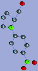
Figure 1: The molecular compound of NPP.

NPP $(C_{11}H_{14}N_{2}O_{3})$ (Fig.1) crystallizes in the solid state in an acentric monoclinic (with space group $P2_{1}$) structure and their parameters are:a=5.261$A^{\circ}$,b=14.908$A^{\circ}$,c=7.185$A^{\circ}$ ,$\beta$=105.18^∘ and in the wavelength range of 0.5 to 2$\mu$m is transparent. The most interesting property of NPP crystal is the proximity of the mean plane of molecule with the crystallographic plane (101); the angle between both of these planes being 11^∘. Nitro group of one molecule in downward connects to Prolinol group in upper by hydrogen bonding. The angle between b orientation of crystal and N(1)-N(2) axis (charge-transfer axis) is equal to 58.6^∘ [8]. Fig. 2 shows the crystal packing of the NPP.

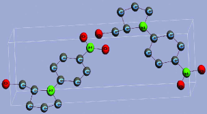
Figure 2: The crystal packing of NPP.

For accurate and valid simulation, these properties and angles have to be exerted. For benzene molecule, benzene ring is a circle (see fig.3);

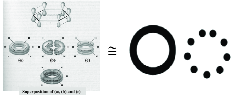
Figure 3: Electron cloud for Benzene molecule that obtained from Huckle theory [37] and its approximation.

Fig.4 demonstrates

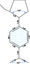
Figure 4: The bond lengths (in angstrom) and angles of NPP molecule.

the bond lengths and angles of the NPP molecule. As we see in this figure the bond lengths in benzene ring are not same. In our simulation, for similarity we consider an ellipse correspond to circle for electron cloud. We obtained $\varepsilon$=0.26 for the ellipse of NPP from simulation, fig.5 shows the comparison of a circle and an ellipse with $\varepsilon$=0.26.

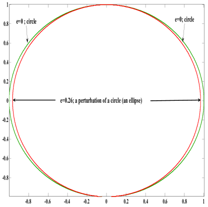
Figure 5: The comparison between circles for Benzene molecule electron cloud and NPP molecule electron cloud, (approximately). As we see the electron cloud of $\pi-$electron in NPP has distorted a little.

3 Our Model for Electro-Optic Effect

For a biaxial crystal that $n_{x}\neq n_{y}\neq n_{z}$ the equation of index ellipsoid is

$$\frac{x^{2}}{n_{x}^{2}}+\frac{y^{2}}{n_{y}^{2}}+\frac{z^{2}}{n_{z}^{2}}=1$$ (1)

Assume that single crystal film lies in x-y plane and light propagation is in the direction; therefore in the presence of an electric field the equation of index ellipsoid by assuming crystal symmetry will become:

$$[(\frac{1}{n^{2}})_{{}_{x}}+r_{12}E_{y}]x^{2}+[(\frac{1}{n^{2}})_{{}_{y}}+r_{22}E_{y}]y^{2}+2r_{61}E_{x}xy=1$$ (2)

for NPP that $E_{x}$ and $E_{y}$ are transverse electric field components, [10]. For MNA crystal Eq.(2) will become:

$$[(\frac{1}{n^{2}})_{{}_{x}}+r_{11}E_{x}]x^{2}+[(\frac{1}{n^{2}})_{{}_{y}}+r_{21}E_{x}]y^{2}$$

$${}+[(\frac{1}{n^{2}})_{{}_{z}}+r_{31}E_{x}]z^{2}+2r_{51}E_{x}xz=1$$

where $E_{x}$ is only transverse electric field component [21]. With appropriate rotational transformation, these relations can been simplified. In NPP, $r_{12}$ and $r_{22}$ and in MNA, $r_{11}$ and $r_{21}$ is large coefficient. Therefore $n_{x}$ and $n_{y}$ for NPP simplified to $n_{x}-(1/2)n_{x}^{3}r_{12}E_{y}$ and $n_{y}-(1/2)n_{y}^{3}r_{22}E_{y}$ and for MNA $n_{x}-(1/2)n_{x}^{3}r_{11}E_{x}$ and $n_{y}-(1/2)n_{y}^{3}r_{21}E_{x}$ respectively. The phase retardation $\Gamma$, with an applied electric field in a typical linear transverse electrooptic modulator will be obtained as follows, [38]:

$$\Gamma=\acute{\phi_{y}}-\acute{\phi_{x}}=\frac{\omega l}{c}\cdot[n_{y}-n_{x}-\frac{1}{2}(n_{y}^{3}r_{22}-n_{x}^{3}r_{12})E_{y}]$$ (4)

for NPP and

$$\Gamma=\acute{\phi_{y}}-\acute{\phi_{x}}=\frac{\omega l}{c}\cdot[n_{y}-n_{x}-\frac{1}{2}(n_{x}^{3}r_{11}-n_{y}^{3}r_{21})E_{x}]$$ (5)

for MNA crystal. The total phase difference between two perpendicular polarization of light (in our example $E_{x}$ and $E_{y}$),is

$$\Delta=\Delta_{0}+\delta$$ (6)

where $\Delta_{0}$ is due to linear birefringence and $\delta$ is due to linear electro-optic effect. In this case $\delta$ is much smaller than $\Delta_{0}$.
In sub-micron space scales and sub-femtoseconds time scales, the optical constants loses its stabilization and classical equations for linear and nonlinear optical phenomena are not useful [45]. Now, we suggest a microscopic model for linear electro-optic phenomenon. If we have a monochromatic laser beam with frequency $\nu$ and intensity I, then we may attain average photon flux from relation [39]:

$$\phi=\frac{I}{h\nu}$$ (7)

now if we assume thin single crystal film of NPP in $"b"$ direction of crystal (or $"z"$ axis) radiated by a He-Ne laser with: $\lambda$=633 nm, average power=10mw and beamwidth=20 microns, then from (4) average photon flux is equal to $10^{22}photons/(s-cm^{2})$ that signifies in every second $10^{22}$ photons arrive to each centimeter square. Moreover from data of crystal in subsection $(A)$ in every 36.5$(A^{\scriptstyle{\circ^{2}}})$ on z direction, one NPP molecule exists. Therefore in every second $36.5\times 10^{6}$ photons interact with any molecule or in other words in every 27ns, (with assuming only linear optic phenomenon exist and nonlinear optic phenomenon do not exist, approximately. Because laser watt is not much), one photon interacts with any NPP molecules. In each interaction between photon and electron in every layer of crystal, we suppose a delay time equal to $\tau_{i}$ ($i$th layer of the crystal). Total delay time for m layers in crystal region is equal to:

$$\sum_{i=1}^{m}\tau_{i}$$

Consequently required time for photon transmission in L length of crystal is equal to $\tau$, achieved from relation:

$$\tau=\frac{L}{\frac{c_{0}}{n}}=\frac{nL}{c_{0}}=\frac{L}{c_{0}}+\sum_{i=1}^{m}\tau_{i}$$ (8)

where $c_{\scriptscriptstyle{0}}$ is velocity of light in vacuum. By using this relation, we can relate macroscopic quantity $n$ to microscopic quantity $\tau_{i}$. In biaxial crystals, $\tau$ and consequently $n$ depends on polarization direction of incident light. Because dipole-field interaction conclusion is different for any direction of molecule. If $\tau_{x}$ would be a microscopic delay for interaction of $x$-polarization field with dipole (or charge transfer action) and $\tau_{y}$ would be a microscopic delay for interaction of $y$-polarization field with dipole then the final phase difference between these two fields (named phase retardation) will be:

$$\Delta\phi=\omega\cdot(\tau_{x}-\tau_{y})=\omega\cdot\sum_{i}(\tau_{x_{i}}-\tau_{y_{i}})$$ (9)

Of course this relation give $\Delta_{0}$ of (6). We justify $\delta$ from our model in later subsections.

4 Photon-Electron Interaction in Attosecond Regime

For analyzing the interaction of the electric field of the photons with $\pi$-electron system, the time-dependent Schroedinger equation has to be used:

$$H(r,t).\Psi(r,t)=\imath\hbar\frac{\partial\Psi(r,t)}{\partial t}$$ (10)

with the Hamilton operator H representing the total energy of the matter-light system and the wave function $\Psi$ representing the quantum state of this system with all detailed spatial and temporal information of all particles in it. First, the stationary Schrodinger for matter without any external interaction is usually applied:

$$H_{matter}(r).\varphi_{m}(r)=E_{m}.\varphi_{m}(r)$$ (11)

The interaction of the photon field with $\pi$-electron system can be described by first-order perturbation theory. The Hamiltonian of (10) is split into the material steady-state Hamiltonian of (11) and the Hamiltonian of the interaction as a small disturbance:

$$H(r,t)=H_{matter}+H_{interaction}(t)$$ (12)

With this equation the temporal change of the coefficient describing the transitions of the the particle under the influence of the light can be calculated from:

$$\frac{\partial}{\partial t}c_{p}(t)=-\frac{\imath}{\hbar}\sum_{m=1}^{\infty}[c_{m}(t).\int_{V}\psi_{p}^{*}H_{interaction}\psi_{m}dV]$$ (13)

with the integration over the whole volume V of the wavefunctions. The probability of the population of state p is given by the square of $c_{p}$ and the transition probability $\omega_{p\leftarrow m}$ for the transition from state m to state p is given by:

$$\omega_{p\leftarrow m}=\frac{\partial}{\partial t}|c_{p}(t)|^{2}\propto\mu_{p\leftarrow m}^{2}$$ (14)

wich is proportional to the square of the transition dipole moment $\mu_{p\leftarrow m}$:

$$\mu_{p\leftarrow m}=\int_{V}\varphi_{p}^{*}.H_{interaction}.\varphi_{m}dV$$ (15)

The interaction operator is given for a one-electron system in the dipole approximation, assuming a radiation wavelength large compared to the dimension of the particle, by:

$$H_{interaction}(t)=-erE(r_{particle})$$ (16)

with the electric charge e, the position of the particle center at $r_{particle}$ and $r$ as the relative position of the charge from the particle center and the electric field vector $E$. For more general case, including large molecules the electric field can be better expressed with the vector potential $A(r,t)$ which is source free:

$$\nabla\cdot A(r,t)=0$$ (17)

and the electric field follows from this potential by:

$$E(r,t)=-\frac{1}{c}.\frac{\partial}{\partial t}A(r,t)$$ (18)

and the magnetic field by:

$$H(r,t)=rotA(r,t)$$ (19)

With respect to the quantum description, the vector potential can be written as:

$$A(r,t)=\sum_{m}e_{m}\sqrt{\frac{h\lambda_{m}}{8\pi^{2}V\varepsilon_{0}c_{0}}}[b_{m}e^{\imath k_{m}r}+b_{m}^{+}e^{-\imath k_{m}r}]$$ (20)

with the counter $m$ for the different waves of light and thus of the electric field, $e_{m}$ as the direction of the field vector, $\lambda_{m}$ as the wavelength of the light wave, V as the volume the waves are generated in and $k_{m}$ as the wave vector of the mth wave. The $b_{m}$ and $b_{m}^{+}$ are photon absorbtion and emission operators which would be light amplitudes in the classical case. These operators fulfill the following relations:

$$b_{m}.b_{p}^{+} - b_{p}^{+}.b_{m}=\delta_{mp}$$

$$b_{m}.b_{p} - b_{p}.b_{m}=0$$

$$b_{m}^{+}.b_{p}^{+} - b_{m}^{+}.b_{m}^{+}=0$$ (21)

which result in the description of the energy of the electrical field by a sum over harmonic oscilators as:

$$H_{field}=\sum_{m}b_{m}^{+}b_{m}h\nu_{m}$$ (22)

and the Hamilton operator for a single electron in the potential of the cores V and the electric field $\bf{A}$ is given by:

$$H_{electron}=\frac{1}{2m_{electron}}.[p-e_{e}A(r,t)]^{2}+V(r,t)$$ (23)

with the mass $m_{electron}$ and charge $e_{e}$ of the electron and the pulse operator:

$$p=-\frac{\imath}{\hbar}\nabla$$ (24)

With these definitions the interaction operator for a one-electron system follows from:

$$H_{interaction}(r,t) = -\frac{e_{e}}{m_{electron}}A(r,t).p$$ (25)

$${}+\frac{e_{e}^{2}}{2m_{electron}}A^{2}(r,t){}$$

for linear interactions the second term can be neglected. But the interaction has to be considered for all charges in the particle which are in molecules for all molecules and core charges. The resulting interaction operator is given by:

$$H_{interaction}(r,t) = \sum_{p}[-\frac{e_{e}}{m_{electron}}A(r_{p},t).p_{p}]$$

$$= +\sum_{q}[-\frac{Z_{core,q}e_{e}}{M_{core}}A(R_{q},t).P_{q}]$$

with the charge $Z_{core,q}$ of the qth core, the coordinate $R_{q}$ of this core and its momentum $P_{q}$. In the dipole approximation the interaction operator for such a system can be written as:

$$H_{interaction}(r,t)=\sum_{m}[-\frac{Z_{charge,m}e_{e}}{m_{charge,m}}E(r_{p},t)]$$ (27)

and thus the transition dipole moment in the dipole approximation follows as:

$$\mu_{p\leftarrow m}=e_{e}.\int_{V}\varphi_{p}^{*}.(\sum_{m}[-\frac{Z_{charge,m}e_{e}}{m_{charge,m}}E(r_{p},t)]).\varphi_{m}dV$$ (28)

For a real material such as NPP or MNA this formula would be very complicated and take enormous calculations. Therefore some approximation must be applied. It can be shown that for absorbtion or emission of photons the material has to perform a transition between two eigenstates $E_{m}$ and $E_{p}$ of the material and thus the photon energy $E_{photon}$ has to fulfill the resonance condition:

$$E_{photon}=h\nu_{photon}=|E_{p}-E_{m}|$$ (29)

But for our linear phenomenon, the photon energy is about $2eV$ (in $\lambda=630nm$). If electron would be in HOMO (Highest Occupied Molecular Orbital), this electron do not go to LUMO (Lowest Unoccupied Molecular Orbital) or exited state by interaction. This phenomena is named nonresonant phenomenon,[9, 40, 41] (nonresonant phenomena is not exclusive for nonlinear optical phenomena). Therefor electron after interaction, go to quasi states that their life times is very short, then this electron go back to primary state after very short time. The nonresonant lifetime is determined by the uncertainty principle and the energy mismatch between photon energy in second time and the input photon energy. We can assume that the characteristic response time of this process is the time required for the electron cloud to become distorted in response to an applied optical field. This response time can be estimated as the orbital period of the electron in its motion around the nucleus which is about $\tau\simeq 10^{-16}s$ or 100as,[41]. We can estimate this characteristic response time according to (9) if, $n=3,L=3\mu$. Consequently $\Sigma\tau$ is equal to $10^{-14}$sec. Because in b direction of crystal in $3\mu$m length, approximately 4024 molecules exist, therefore the average quantity of $\tau$:

$$\overline{\tau}=\frac{\sum\tau}{N}$$

is in order of $10^{-18}s$ or 1 as. The perturbation in this very short time can assume semiclassically. In linear phenomenon in this short time, just one photon interacts with one molecule. Because NPP molecule has delocalization electrons,(or $\pi$-electron system), in benzene ring, that photon interacts with this electron type,[32] and it is annihilated [38]. We call this photon, a successful photon, (that does not produce phonon).
To obtain $\pi$-electron wavefunction for benzene molecule the Schrödinger equation may be solved. Since this is very complicated process, it cannot be done exactly, an approximated procedure known as Hückle method must be employed. In this method, by using Hückle Molecular-Orbital (HMO) calculation, a wave function is formulated that is a linear combination of the atomic orbitals (LCAO) that have overlapped [37] (see Fig.3):

$$\Psi=\sum_{i}C_{i}\Phi_{i}$$ (30)

where the $\Phi_{i}$ refers to atomic orbitals of carbon atoms in the ring and the summation is over the six C atoms. The coefficients of the atomic orbitals are calculated self-consistently through Roothaan’s equations to obtain the $\Psi$ and the corresponding the one electron energies $\epsilon$, [43]:

$$\sum_{\nu}(F_{\mu\nu}-\epsilon.S_{\mu\nu})C_{\nu}=0,$$ (31)

where the Fock matrix $F_{\mu\nu}$ and overlap integrals $S_{\mu\nu}$ are given by:

$$F_{\mu\nu}=H_{\mu\nu}+\sum_{\lambda\sigma}P_{\lambda\sigma}[(\mu\nu|\lambda\sigma)-\frac{1}{2}(\mu\lambda|\nu\sigma)]$$ (32)

and

$$S_{\mu\nu}=\int\phi_{\mu}.\phi_{\nu}d\tau$$ (33)

Here the core Hamiltonian matrix $H_{\mu\nu}$, density matrix $P_{\mu\nu}$, and two-electron repulsion integrals are given by:

$$H_{\mu\nu}=\int\phi_{\mu}H^{core}\phi_{\nu}d\tau,$$ (34)

$$P_{\mu\nu}=2\sum_{i=1}^{occupied}C_{\mu i}C_{\nu i},$$ (35)

and

$$(\mu\nu|\lambda\sigma)=\int\phi_{\mu}(1)\phi_{\nu}(1)\frac{1}{r_{12}}\phi_{\lambda}(2)\phi_{\sigma}(2)d\tau_{1}d\tau_{2},$$ (36)

and the molecular Hamiltonian by

$$H=\sum_{i}H_{i}^{core}+\sum_{i<j}\frac{1}{r_{ij}},\ H_{i}^{core}=-\frac{1}{2}\nabla_{i}^{2}-\sum_{A}\frac{Z_{A}}{r_{Ai}}$$ (37)

where the sum on $i(A)$ is over electrons (nucleii), and the $Z_{A}$ is the net core charge. The $|C_{i}|^{2}$ is the probability of the $\pi$-electron at $i$th atom. Thus:

$$|C_{1}|^{2}+|C_{2}|^{2}+|C_{3}|^{2}+|C_{4}|^{2}+|C_{5}|^{2}+|C_{6}|^{2}=1$$

In the case of Benzene molecule:

$$|C_{i}|^{2}=\frac{1}{6}$$

as followed from the symmetry of the ring [44, 45]. But NPP and MNA molecules aren’t such as Benzene molecule. NPP is polar molecule. Nitro $(NO_{2})$ is more powerful electronegative compound than prolinol and pulls $\pi$-electron system; consequently, the probability of finding $\pi$-electron system at various carbon atoms of main ring isn’t the same and the probability of finding $\pi$-electrons near the Nitro group is greater than near the prolinol group. Therefore there is no symmetry for NPP and electron cloud is spindly or oblong, (similar to dom-bell) (Fig.6).

Figure 6: Assumed $\pi$-electron orbit of NPP molecule that obtained from fig. 3 for Benzene molecule (approximately).

We estimate this form of electron cloud by an ellipse that our calculations would be uncomplicated. We assume effective positive charge that is located in one of focal points of ellipse. The quantity of this effective positive charge is determined by semiclassical arguments. For attaining probability of electron presence on an orbit (Fig.7),

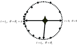
Figure 7: $\pi$-electron system approximation for NPP molecule, $\theta$ = 0 is in the positive direction of dipole (Prolinol side) and $\theta$ = $\pi$ is in the negative direction of dipole (Nitro side).

we say, T time is required by radial vector to sweep total $\pi.u.v$ interior area of ellipse (u and v are semimajor and semiminor axis of ellipse respectively), in t times, this radial vector sweeps:

$$\pi.u.v.\frac{t}{T}$$

area of ellipse, (see Fig.7). If t is the time, that electron sweeps $\theta$ radian of orbit then t is obtained from this relation [32]:

$$t=\frac{T}{2\pi}\{2\arctan(\sqrt{\frac{1-\varepsilon}{1+\varepsilon}}\tan(\frac{\theta}{2}))-\frac{\varepsilon.\sqrt{1-\varepsilon^{2}}.\sin(\theta)}{1+\varepsilon.\cos(\theta)}\}$$ (38)

Where $\varepsilon$ is ellipse eccentricity. By using this relation, we attain the required time (t) for electron to traverse from $\theta$ to $\theta+d\theta$ and it is divided by total time T. By this approach, we can determine the PDF (Probability Density Function) approximately. The PDF in apogee (near the Nitro group), is maximum and in perigee (near the Prolinol or Methane) is minimum. Therefore PDF is correlated to $\theta$ from (38) and seen in Fig.8.

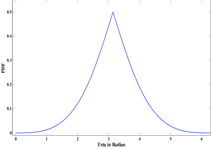
Figure 8: PDF of presence probability of $\pi$-electron in different energy states when it rotates around the assumed orbit in Fig.7; as we see the PDF is correlated to $\theta$.

The $\tau$ quantity is correlated to $\theta$ and consequently, $\tau$ quantity is correlated to presence probability of $\pi$-electron system.
The angle between Y vector and charge transfer action (N₁-N₂) is 58.6^∘ and X and Z axis is perpendicular to Y (Fig.9).

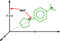
Figure 9: X, Y and Z axis and NPP molecule in dielectric frame.

We consider propagation along Z direction. We spot a photon interacts with $\pi$-electron of NPP in first layer. After interaction, this photon gives its energy to electron and is annihilated. Electron absorbs energy and digresses in direction of photon momentum. Electron with photon energy, may not be unbounded and after arriving to apogee of digression, it returns back to ground state, because the photon energy is equal to $h\nu=1.96ev$ (h is Planck’s constant and $\nu$ is frequency of laser beam) whereas energy for excitation is greater than $3ev$. When electron returns to ground state one photon is produced. The time coming up and down is $\tau$ delay time. This photon after freedom goes to second layer in direction of annihilated photon (nonce, we assume the polarization doesn’t change), in second layer this photon interacts with another delocalization $\pi$-electron certainly, because the effective interaction range of photon is approximately equal to its wavelength and is very greater than the distance between molecules. This molecule is nearest to photon effective central. This action is repeated for each layer. The location of photon-electron interaction is significant in every molecule and it is effective on $\tau$ quantity directly. We assume that interacting photon has circle polarization and electron subject to virtual positive charge center. The phase retardation between $E_{x}$ and $E_{y}$ (9) can be obtain from this relation,[32]:

$$\Delta\phi=\frac{\omega.\sqrt{2h\nu.m}}{KZe^{2}}\sum_{i=1}^{m}[\cos(\theta_{i})-\sin(\theta_{i})].r_{i}^{2}$$ (39)

that

$$r_{i}=\frac{(1-\epsilon^{2}).u}{1+\epsilon.\cos(\theta_{i})}$$

where $\epsilon$ is the elliptical eccentricity and u is the semimajor axis of the ellipse. By applying an external transverse electric field to organic crystal (in the range of several volts per micron) the shape of $\pi$-electron system will be deformed slightly and we would be expect some noticeable variations in microscopic delay parameters ($\tau_{x}$,$\tau_{y}$) and phase retardation; (see Fig.10).

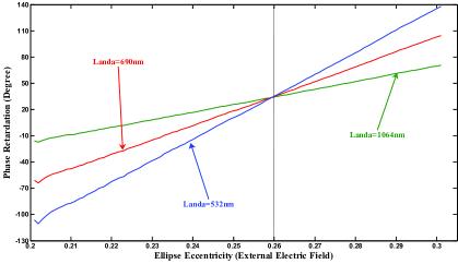
Figure 10: Phase retardation between $E_{x}$ and $E_{y}$ of optical signal with different wavelength by applied external electric field. As we see; by applied electric field, the virtual ellipse eccentricity change (electron in electrical field). With eccentricity variation, the microscopic delay ($\tau_{x}$,$\tau_{y}$) change and consequently phase retardation is modified.

Consequently, by step-like change of input voltage, optical signal is switched between output port of DOS.

5 Variation Analysis of Phase Retardation versus Applied Electric Field

We simulate phase retardation of $3\mu m$-length NPP crystal by Monte-Carlo method, then we generate random number using $MATLAB$ program. This program produces PDF quantities was explained in before subsection and relates each of them to every molecule. These values are indexing $\pi$-electron positions in each layer, by assumption a reference point (see fig. 6). Additionally we have used a $MATLAB$ program for Monte-Carlo simulation. The inputs of this program are:
1. The wavelength of incident optical beam in which we want to design DOSs;
2. $h,m,q,k=\frac{1}{4\pi.\varepsilon},c_{\scriptscriptstyle{0}}$ that are Planck’s constant, electron rest mass, elementary charge, Coulomb constant and speed of light respectively.
3. Unit cell parameters of NPP crystal: a, b, c, $\beta$ and its other parameters that have given in subsection (A).
4. L: crystal thickness that in our simulation it is 3$\mu$m.
And the outputs of $MATLAB$ program are: phase retardation in each wavelength.
System calibration is done semiclassically by experimental refractive index data.t In this method that we obtain three refractive indexes with x-polarization in threea with $\epsilon$ (eccentricity), u (semimajor axis of ellipse) and Z (equivalent positive charge) in a way that refractive indexes in three wavelengths are very close to experimental data. Then we would see that refractive index in other wavelengths and other polarization with same $\epsilon$, u and Z will be achieved. Of course these values, $\epsilon$, u and Z would be close to experimental structure of crystal, for example u would be greater than and smaller than minimum and maximum sizes of six lengths of benzene hexagonal respectively, or $\epsilon$ would be small but greater than zero. In other hand these values must be logical. From this method in our simulation we have obtained $\epsilon=0.26,Z=3.9,u=1.4A^{0}$ that is very close to experimental and structural data.
Xu and co-workers [19, 26], have done some electro-optic experiment about single crystal film of NPP. They have obtained $|n_{x}^{3}r_{12}-n_{y}^{3}r_{22}|=340pm/V$ and $r_{12}=65pm/V$ in an optical beam with 1064nm wavelength. They have studied phase retardation between $E_{x}$ and $E_{y}$ of optical beam as a function of angle between electric field and charge transfer action of NPP. They have concluded that the maximum phase retardation was observed for the field oriented along the charge-transfer axis which was parallel to the film surface. The electro-optic effect or phase retardation was negligible when the electric field was applied perpendicular to the charge-transfer axis. This concept could be justified by our model in previous subsection. When the angle between charge-transfer action and external electric field change, the ellipse eccentricity modify and consequently, the phase retardation alter. Obviously, from Fig.5 when the external electric is parallel to charge-transfer axis, the ellipse drag more and the ellipse convert to a line. Therefor, ellipse eccentricity arise and from Fig.9 the phase retardation growth. In the other hand, from Fig.5 when the angle between external electric field and charge-transfer axis change, the ellipse is gathered and convert to circle and the eccentricity decrease to zero. Thus from Fig.9 the phase retardation is lowered.

6 Conclusion

we justified linear EO phenomenon by QPM. This suggested physical model could be a powerful tool for analyzing and explaining processes that happen in waveguides with microscopic and nanoscopic sizes. We showed how the phase retardation between different arguments of an optical field with distinctive wavelengths can take place.

References

- [1] Lee M H, Min Y H, Ju J J, Do J Y and Park S K 2001 IEEE J. Sel. Top. Quantum Electron. 7 5
- [2] Oh M, Zhang H, Erlig H, Chang Y, Tsap B, Chang D, Szep A, Steier W H, Fetterman H R and Dalton L R 2001 IEEE J. Sel. Top. Quantum Electron. 7 5
- [3] Yuan W, Kim S, Steier W H and Fetterman H R 2005 IEEE Photon. Technol. Lett. 17 12
- [4] Yuan W, Kim S, Sadowy G, Zhang C, Wang C, Steier W H and Fetterman H R 2004 Electron. Lett.40 3
- [5] Lee S S, Shin S Y 1999 Electron. Lett. 35 15
- [6] Lee S S, Shin S Y 1997 Electron. Lett. 33 4
- [7] Ahn J T, Park S, Do J Y, Lee J M, Lee M H and Kim K H 2004 IEEE Photon.Technol. Lett. 16 6
- [8] Zyss J, Nicoud J F and Coquillay M 1984 J. Chem. Phys. 81 4160
- [9] Nalwa H and Miyata 1997 Nonlinear optics of organic molecules and polymers (Hitachi research Laboratory and Tokyo University of Agriculture and Technology)
- [10] Xu J, Zhou L and Thakur M 1996 Appl. Phys. Lett. 69 1197
- [11] Ledoux I, Lepers C, Perigaud A, Badan J and Zyss J 1990 Opt. Commun. 80 149
- [12] Ledoux I, Josse D, Vidakovic P and Zyss J 1986 Opt. Eng. 25 202
- [13] Banfi G P, Datta P K, Degiorgio V, Fortusini D, Shepherd E E A and Sherwood J N 1999 Chem. Phys. 245
- [14] Datta P K, Fortusini D, Donelli G, Banfi G P, Degiorgio V, Sherwood J N and Bhar G C 1998 Opt. Commun. 149
- [15] Banfi G P, Degiorgio V, Sherwood J N 2001 Synthetic Metals 124
- [16] Quintero-Torres R and Thakur M 1996 Appl. Phys. Lett. 69
- [17] Xu J, Zhou L and Thakur M 1998 Appl. Phys. Lett. 72
- [18] Vallee R, Damman P, Dosiere M and Zyss J 2001 J. Chem. Phys. 115
- [19] Levine B F, Bethea C G, Thurmond C D, Lynch R T and Bernstein J L 1979 J. Appl. Phys. 50 4
- [20] Khanarian G, Che T, Demartino R N, Haas D, Leslie T, Man H T and Sasone M 1987 SPIE Advances in Nonlinear Polymers and Inorganic Crystals, Liquid Crystals and Laser Media 824
- [21] Ho E S S, Iizuko K, Freundorfer A P and Wah C K L 1991 J. Lightwave Technol. 9 1
- [22] Jurgen R and Meyer-Arendi M D 1984 Introduction to Classic and Modern Optics (2nd ed. Prentice Hall Inc.)
- [23] Feynman R P, Leighton R B and Sands M 1963 The Feynman Lectures on Physics (Addison-Wesley Publishing Company)
- [24] Feynman R P 1985 QED: The Strange Theory of light and Matter(Penguin Books)
- [25] Marcuse D 1970 Engineering Quantum Electrodynamics(Hardcourt Brace and World Inc.)
- [26] Jensen B 1982 IEEE J. Quantum. Electron. QE-18 9
- [27] Jensen B and Torabi A 1983 IEEE J. Quantum. Electron. QE-19 3
- [28] Jensen B and Torabi A 1983 IEEE J. Quantum. Electron. QE-19 5
- [29] Huang H, Yee S and Soma M 1990 J. Appl. Phys. 67 4
- [30] Wheeler J A 1933 Phys. Rev. 43
- [31] Simpson S H, Richardson R M and Hanna S 2005 J. chem. Phys. 123
- [32] Kaatuzian H and Wahedy Zarch A A 2004 Proc. of CSIMTA Cherbourg-Normandy-FRANCE
- [33] Kaatuzian H, Bazhdanzadeh N and Ghohrodi Ghamsari B 2004 Proc. of CSIMTA Cherbourg-Normandy-FRANCE
- [34] Kaatuzian H and Wahedy Zarch A A 2006 Proc. CSNDSP2006, Patras Univ, Greece.
- [35] Adibi A and Kaatuzian H 1995 J. of Engineering, Islamic Republic of Iran 8 4
- [36] Williams D J Ed. 1983 Nonlinear Optical Properties of Organic and Polymeric Materials American Chemical Society, ACS symposium series
- [37] March J 1992 Advanced Organic Chemistry: Reactions, Mechanisms and Structure (4th Ed. John Wiley and Sons)
- [38] Yariv A 1975 Quantum Electronics(2nd Ed.) John Wiley and Sons Inc
- [39] Saleh B E A and Teich 1991 Fundamentals of Photonics (2nd Ed. John Wiley and Sons)
- [40] Menzel R 2000 Photonics, Linear and nonlinear interactions of laser light and matter Springer
- [41] Boyd R W 2003 Nonlinear optics(3th Ed.) John Wiley and Sons Inc.
- [42] Dirk C W, Twieg R J and wagniere G 1986 J. Am. Chem. Soc. 108 18
- [43] Lalama S J and Garito A F 1979 Phys. Rev. A 20 3
- [44] Omar M A 1974 Elementary Solid State Physics(Mills and Bons Ltd.)
- [45] Waddington N 1972 Modern Organic Chemistry (Addison-Wesley)