Abstract: Various performance indices are used for the design of serial manipulators. One method of optimization relies on the condition number of the Jacobian matrix. The minimization of the condition number leads, under certain conditions, to isotropic configurations, for which the roundoff-error amplification is lowest. In this paper, the isotropy conditions, introduced elsewhere, are the motivation behind the introduction of isotropic sets of points. By connecting together these points, we define families of isotropic manipulators. This paper is devoted to planar manipulators, the concepts being currently extended to their spatial counterparts. Furthermore, only manipulators with revolute joints are considered here.

1 Introduction

Various performance indices have been devised to assess the kinetostatic performance of serial manipulators. The literature on performance indices is extremely rich to fit in the limits of this paper, the interested reader being invited to look at it in the rather recent references cited here. A dimensionless quality index was recently introduced by Lee, Duffy, and Hunt (1998) based on the ratio of the Jacobian determinant to its maximum absolute value, as applicable to parallel manipulators. This index does not take into account the location of the operation point in the end-effector, for the Jacobian determinant is independent of this location. The proof of the foregoing fact is available in (Angeles, 1997), as pertaining to serial manipulators, its extension to their parallel counterparts being straightforward. The condition number of a given matrix, on the other hand is well known to provide a measure of invertibility of the matrix (Golub and Van Loan, 1989). It is thus natural that this concept found its way in this context. Indeed, the condition number of the Jacobian matrix was proposed by Salisbury and Craig (1982) as a figure of merit to minimize when designing manipulators for maximum accuracy. In fact, the condition number gives, for a square matrix, a measure of the relative roundoff-error amplification of the computed results (Golub and Van Loan, 1989) with respect to the data roundoff error. As is well known, however, the dimensional inhomogeneity of the entries of the Jacobian matrix prevents the straightforward application of the condition number as a measure of Jacobian invertibility. The characteristic length was introduced in (Angeles and López-Cajún, 1992) to cope with the above-mentioned inhomogeneity. Apparently, nevertheless, this concept has found strong opposition within some circles, mainly because of the lack of a direct geometric interpretation of the concept. It is the aim of this paper to shed more light in this debate, by resorting to the concept of isotropic sets of points. Briefly stated, the application of isotropic sets of points to the design of manipulator architectures relies on the concept of distance in the space of $m\times n$ matrices, which is based, in turn, on the Frobenius norm of matrices. With the purpose of rendering the Jacobian matrix dimensionally homogeneous, moreover, we introduce the concept of posture-dependent conditioning length. Thus, given an arbitrary serial manipulator in an arbitrary posture, it is possible to define a unique length that renders this matrix dimensionally homogeneous and of minimum distance to isotropy. The characteristic length of the manipulator is then defined as the conditioning length corresponding to the posture that renders the above-mentioned distance a minimum over all possible manipulator postures.

It is noteworthy that isotropy comprising symmetry at its core, manipulators with only revolute joints are considered here. It should be apparent that mixing actuated revolutes with actuated prismatic joints would destroy symmetry, and hence, isotropy.

2 Algebraic Background

When comparing two dimensionless $m\times n$ matrices A and B, we can define the distance $d({\bf{A}},\,{\bf{B}})$ between them as the Frobenius norm of their difference, namely,

$$d({\bf{A}},\,{\bf{B}})\equiv\|{\bf{A}}-{\bf{B}}\|{\rm~{}~{}i.e.,~{}~{}}d({\bf{A}},\,{\bf{B}})\equiv\sqrt{\frac{1}{n}{\rm tr}[({\bf{A}}-{\bf{B}})({\bf{A}}-{\bf{B}})^{T}]}$$ (1)

An $m\times n$ isotropic matrix, with $m<n$, is one with a singular value $\sigma>0$ of multiplicity $m$, and hence, if the $m\times n$ matrix C is isotropic, then

$${\bf{C}}{\bf{C}}^{T}=\sigma^{2}{\bf{1}}$$ (2)

where 1 is the $m\times m$ identity matrix. Note that the generalized inverse of C can be computed without roundoff-error, for it is proportional to ${\bf{C}}^{T}$, namely,

$$({\bf{C}}{\bf{C}}^{T})^{-1}{\bf{C}}^{T}=\frac{1}{\sigma^{2}}{\bf{C}}^{T}$$ (3)

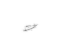
Figure 1.  : Planar $n$-revolute manipulator

Furthermore, the condition number $\kappa({\bf{A}})$ of a square matrix A is defined as (Golub and Van Loan, 1989)

$$\kappa({\bf{A}})=\|{\bf{A}}\|\|{\bf{A}}^{-1}\|$$ (4)

where any norm can be used. For purposes of the paper, we shall use the Frobenius norm for matrices and the Euclidean norm for vectors. Henceforth we assume, moreover, a planar $n$-revolute manipulator, as depicted in Fig. 1, with Jacobian matrix J given by (Angeles, 1997)

$${\bf{J}}=\left[\begin{array}[]{cccc}1&1&\cdots&1\\ {\bf{E}}{\bf{r}}_{1}&{\bf{E}}{\bf{r}}_{2}&\cdots&{\bf{E}}{\bf{r}}_{n}\end{array}\right]{\rm~{}~{},~{}~{}~{}~{}~{}}{\bf{E}}=\left[\begin{array}[]{cc}0&-1\\ 1&0\end{array}\right]$$ (9)

where ${\bf{r}}_{i}$ is the vector directed from the center of the $i$th revolute to the operation point $P$ of the end-effector, and matrix ${\bf{E}}$ represents a counterclockwise rotation of $90^{\circ}$.

It will prove convenient to partition J into a $1\times n$ block A and a $2\times n$ block B, defined as ${\bf{A}}=[1~{}1~{}\cdots~{}1]$ and ${\bf{B}}=[{\bf{E}}{\bf{r}}_{1}~{}{\bf{E}}{\bf{r}}_{2}~{}\cdots~{}{\bf{E}}{\bf{r}}_{n}]$. Therefore, while the entries of A are dimensionless, those of B have units of length. Thus, the sole singular value of A, i.e., the nonnegative square root of the scalar of ${\bf{A}}{\bf{A}}^{T}$, is $\sqrt{n}$, and hence, dimensionless, and pertains to the mapping from joint-rates into end-effector angular velocity. The singular values of B, which are the nonnegative square roots of the eigenvalues of ${\bf{B}}{\bf{B}}^{T}$, have units of length, and account for the mapping from joint-rates into operation-point velocity. It is thus apparent that the singular values of ${\bf{J}}$ have different dimensions and hence, it is impossible to compute $\kappa({\bf{J}})$ as in eq.(4), for the norm of ${\bf{J}}$ cannot be defined. The normalization of the Jacobian for purposes of rendering it dimensionless has been judged to be dependent on the normalizing length (Paden, and Sastry, 1988; Li, 1990). As a means to avoid the arbitrariness of the choice of that normalizing length, the characteristic length $L$ was introduced in (Ranjbaran, Angeles, González-Palacios, and Patel, 1995). We shall resort to this concept, while shedding more light on it, in discussing manipulator architectures.

3 Isotropic Sets of Points

Consider the set ${\cal S}\equiv\{\,P_{k}\,\}_{1}^{n}$ of $n$ points in the plane, of position vectors $\{\,{\bf{p}}_{k}\,\}_{1}^{n}$, and centroid $C$, of position vector c, i.e.,

$${\bf{c}}\equiv\frac{1}{n}\sum_{1}^{n}{\bf{p}}_{k}$$ (10)

The summation appearing in the right-hand side of the above expression is known as the first moment of $\cal S$ with respect to the origin $O$ from which the position vectors stem. The second moment of $\cal S$ with respect to $C$ is defined as a tensor M, namely,

$${\bf{M}}\equiv\sum_{1}^{n}({\bf{p}}_{k}-{\bf{c}})({\bf{p}}_{k}-{\bf{c}})^{T}$$ (11)

It is now apparent that the root-mean square value of the distances $\{\,d_{k}\,\}_{1}^{n}$ of $\cal S$, $d_{\rm rms}$, to the centroid is directly related to the trace of M, namely,

$$d_{\rm rms}\equiv\sqrt{\frac{1}{n}\sum_{1}^{n}({\bf{p}}_{k}-{\bf{c}})^{T}({\bf{p}}_{k}-{\bf{c}})}\equiv\sqrt{\frac{1}{n}{\rm tr}({\bf{M}})}$$ (12)

Further, the moment of inertia I of $\cal S$ with respect to the centroid is defined as that of a set of unit masses located at the points of $\cal S$, i.e.,

$${\bf{I}}\equiv\sum_{1}^{n}[\,\|{\bf{p}}_{k}-{\bf{c}}\|^{2}{\bf{1}}-({\bf{p}}_{k}-{\bf{c}})({\bf{p}}_{k}-{\bf{c}})^{T}\,]$$ (13a)

in which 1 is the $$3\times 3$$ identity matrix. Hence, in light of definitions (11) and (12),

$${\bf{I}}={\rm tr}({\bf{M}}){\bf{1}}-{\bf{M}}$$ (13b)

We shall refer to I as the geometric moment of inertia of $\cal S$ about its centroid. It is now apparent that I is composed of two parts, an isotropic matrix of norm ${\rm tr}({\bf{M}})$ and the second moment of $\cal S$ with the sign reversed. Moreover, the moment of inertia I can be expressed in a form that is more explicitly dependent upon the set $\{\,{\bf{p}}_{k}-{\bf{c}}\,\}_{1}^{n}$, if we recall the concept of cross-product matrix (Angeles, 1997): For any three-dimensional vector v, we define the cross-product matrix ${\bf{P}}_{k}$ of $({\bf{p}}_{k}-{\bf{c}})$, or of any other three-dimensional vector for that matter, as

$${\bf{P}}_{k}\equiv\frac{\partial[({\bf{p}}_{k}-{\bf{c}})\times{\bf{v}}]}{\partial{\bf{v}}}$$ (14a)

Further, we recall the identity (Angeles, 1997)

$${\bf{P}}_{k}^{2}\equiv-\|{\bf{p}}_{k}-{\bf{c}}\|^{2}{\bf{1}}+({\bf{p}}_{k}-{\bf{c}})({\bf{p}}_{k}-{\bf{c}})^{T}$$ (14b)

It is now apparent that the moment of inertia of $\cal S$ takes the simple form

$${\bf{I}}=-\sum_{1}^{n}{\bf{P}}_{k}^{2}$$ (15)

We thus have

Definition 1 (Isotropic Set)

The set $\cal S$ is said to be isotropic if its second-moment tensor with respect to its centroid is isotropic.

As a consequence, we have

Lemma 1

The geometric moment of inertia of an isotropic set of points is isotropic. Conversely, an isotropic geometric moment of inertia pertains necessarily to an isotropic set of points.

We describe below some properties of isotropic sets of points that will help us better visualize the results that follow.

3.1 ISOTROPY-PRESERVING OPERATIONS ON SETS OF POINTS

Consider two isotropic sets of points in the plane, ${\cal S}_{1}=\{\,P_{k}\,\}_{1}^{n}$ and ${\cal S}_{2}=\{\,P_{k}\,\}_{n+1}^{n+m}$. If the centroid $C$ of the position vector ${\bf{c}}$ of ${\cal S}_{1}$ coincides with that of ${\cal S}_{2}$, i.e. if,

$${\bf{c}}\equiv\frac{1}{n}\sum_{1}^{n}{\bf{p}}_{k}\equiv\frac{1}{m}\sum_{n+1}^{n+m}{\bf{p}}_{k}$$ (16)

then, the set ${\cal S}={\cal S}_{1}\cup{\cal S}_{2}$ is isotropic. Hence,

Property 1

The union of two isotropic sets of points sharing the same centroid is also isotropic.

Furthermore, as the reader can visualize, we state below one more operation on sets of points, namely, a rigid-body rotation, that preserves isotropy:

Property 2

The rotation of an isotropic set of points as a rigid body with respect to its centroid is also isotropic.

3.2 TRIVIAL ISOTROPIC SETS OF POINTS

An isotropic set of points can be defined by the union, rotation, or a combination of both, of isotropic sets. The simplest set of isotropic points is the set of vertices of a regular polygon. We thus have

Definition 2 (Trivial isotropic set)

A set of $n$ points ${\cal S}$ is called trivial if it is the set of vertices of a regular polygon with $n$ vertices.

Lemma 2

A trivial isotropic set ${\cal S}$ remains isotropic under every reflection about an axis passing through the centroid $C$.

4 An Outline of Kinematic Chains

The connection between sets of points and planar manipulators of the serial type is the concept of simple kinematic chain. For completeness, we recall here some basic definitions pertaining to this concept.

4.1 SIMPLE KINEMATIC CHAINS

The kinematics of manipulators is based on the concept of kinematic chain. A kinematic chain is a set of rigid bodies, also called links, coupled by kinematic pairs. In the case of planar chains, two lower kinematic pairs are possible, the revolute, allowing pure rotation of the two coupled links, and the prismatic pair, allowing a pure relative translation, along one direction, of the same links. For the purposes of this paper, we study only revolute pairs, but prismatic pairs are also common in manipulators.

Definition 3 (Simple kinematic chain)

A kinematic chain is said to be simple if each and every one of its links is coupled to at most two other links.

A simple kinematic chain can be open or closed; in studying serial manipulators we are interested in the former. In such a chain, we distinguish exactly two links, the terminal ones, coupled to only one other link. These links are thus said to be simple, all other links being binary. In the context of manipulator kinematics, one terminal link is arbitrarily designated as fixed, the other terminal link being the end-effector (EE), which is the one executing the task at hand. The task is defined, in turn, as a sequence of poses—positions and orientations—of the EE, the position being given at a specific point $P$ of the EE that we term the operation point.

4.2 ISOTROPIC KINEMATIC CHAINS

To every set $\cal S$ of $n$ points it is possible to associate a number of kinematic chains. To do this, we number the points from 1 to $n$, thereby defining $n-1$ links, the $i$th link carrying joints $i$ and $i+1$. Links are thus correspondingly numbered from 1 to $n$, the $n$th link, or EE, carrying joint $n$ on its proximal (to the base) end and the operation point $P$ on its distal end. Furthermore, we define an additional link, the base, which is numbered as 0.

It is now apparent that, since we can number a given set $\cal S$ of $n$ points in $n!$ possible ways, we can associate $n!$ kinematic chains to the above set $\cal S$ of $n$ points. Clearly, these chains are, in general, different, for the lengths of their links are different as well. Nevertheless, some pairs of identical chains in the foregoing set are possible.

Definition 4 (Isotropic kinematic chain)

Let set $\cal S$ of $n$ points be iso-tropic, and the operation point $P$ be defined as the centroid of $\cal S$. Any kinematic chain stemming from $\cal S$ is said to be isotropic.

5 The Posture-Dependent Conditioning Length of Planar n-Re-volute Manipulators

Under the assumption that the manipulator finds itself at a posture $\cal P$ that is given by its set of joint angles, $\{\,\theta_{k}\,\}_{1}^{n}$, we start by dividing the last two rows of the Jacobian by a length $l_{\cal P}$, as yet to be determined. This length will be found so as to minimize the distance of the normalized Jacobian to a corresponding isotropic matrix K, subscript $\cal P$ reminding us that, as the manipulator changes its posture, so does the length $l_{\cal P}$. This length will be termed the conditioning length of the manipulator at $\cal P$.

5.1 A DIMENSIONALLY-HOMOGENEOUS JACOBIAN MATRIX

In order to distinguish the original Jacobian matrix from its dimensionally-homogeneous counterpart, we shall denote the latter by $\overline{{\bf{J}}}$, i.e.,

$$\overline{{\bf{J}}}=\left[\begin{array}[]{cccc}1&1&\cdots&1\\ (1/l_{\cal P})~{}{\bf{E}}{\bf{r}}_{1}&(1/l_{\cal P})~{}{\bf{E}}{\bf{r}}_{2}&\cdots&(1/l_{\cal P})~{}{\bf{E}}{\bf{r}}_{n}\end{array}\right]$$ (19)

Now the conditioning length will be defined via the minimization of the distance of the dimensionally-homogeneous Jacobian matrix $\overline{{\bf{J}}}$ of an $n$-revolute manipulator to an isotropic $3\times n$ model matrix K whose entries are dimensionless and has the same gestalt as any $3\times n$ Jacobian matrix. To this end, we define an isotropic set ${\cal K}=\{\,K_{i}\,\}_{1}^{n}$ of $n$ points in a dimensionless plane, of position vectors $\{\,{\bf{k}}_{i}\,\}_{1}^{n}$, which thus yields the dimensionless matrix

$${\bf{K}}=\left[\begin{array}[]{cccc}1&1&\cdots&1\\ {\bf{E}}{\bf{k}}_{1}&{\bf{E}}{\bf{k}}_{2}&\cdots&{\bf{E}}{\bf{k}}_{n}\end{array}\right]$$ (22)

Further, we compute the product ${\bf{K}}{\bf{K}}^{T}$:

$${\bf{K}}{\bf{K}}^{T}=\left[\begin{array}[]{cc}n&\sum_{1}^{n}{\bf{k}}_{i}^{T}{\bf{E}}^{T}\\ \sum_{1}^{n}{\bf{E}}{\bf{k}}_{i}&\sum_{1}^{n}{\bf{E}}{\bf{k}}_{i}{\bf{k}}_{i}^{T}{\bf{E}}^{T}\end{array}\right]$$ (25)

Upon expansion of the summations occurring in the above matrix, we have

$$\sum_{1}^{n}{\bf{k}}_{i}^{T}{\bf{E}}^{T}=(\sum_{1}^{n}{\bf{E}}{\bf{k}}_{i})^{T}={\bf{E}}(\sum_{1}^{n}{\bf{k}}_{i})^{T}{\rm~{}and~{}}\sum_{1}^{n}{\bf{E}}{\bf{k}}_{i}{\bf{k}}_{i}^{T}{\bf{E}}^{T}={\bf{E}}(\sum_{1}^{n}{\bf{k}}_{i}{\bf{k}}_{i}^{T}){\bf{E}}^{T}$$

Now, by virtue of the assumed isotropy of $\cal K$, the terms in parentheses in the foregoing expressions become

$$\sum_{1}^{n}{\bf{k}}_{i}={\bf{0}}{\rm~{}~{}~{}and~{}~{}~{}~{}}\sum_{1}^{n}{\bf{k}}_{i}{\bf{k}}_{i}^{T}=k^{2}{\bf{1}}_{2\times 2}$$

where the factor $k^{2}$ is as yet to be determined and ${\bf{1}}_{2\times 2}$ denotes the $2\times 2$ identity matrix. Hence, the product ${\bf{K}}{\bf{K}}^{T}$ takes the form

$${\bf{K}}{\bf{K}}^{T}=\left[\begin{array}[]{cc}n&{\bf{0}}^{T}\\ {\bf{0}}&k^{2}{\bf{1}}_{2\times 2}\end{array}\right]$$ (28)

Now, in order to determine $k^{2}$, we recall that matrix K is isotropic, and hence that the product ${\bf{K}}{\bf{K}}^{T}$ has a triple eigenvalue. It is now apparent that the triple eigenvalue of the said product must be $n$, which means that

$$k^{2}=n{\rm~{}~{}~{}and~{}~{}~{}}\sum_{1}^{n}{\bf{k}}_{i}{\bf{k}}_{i}^{T}=(n){\bf{1}}_{2\times 2}$$ (29)

5.2 COMPUTATION OF THE CONDITIONING LENGTH

We can now formulate a least-square problem aimed at finding the conditioning length $l_{\cal P}$ that renders the distance from $\overline{{\bf{J}}}$ to K a minimum. The task will be eased if we work rather with the reciprocal of $l_{\cal P}$, $\lambda\equiv 1/l_{\cal P}$, and hence,

$$z\equiv\frac{1}{2}\frac{1}{n}{\rm tr}[(\overline{{\bf{J}}}-{\bf{K}})(\overline{{\bf{J}}}-{\bf{K}})^{T}]\quad\rightarrow\quad\min_{\lambda}$$ (30)

Upon simplification, and recalling that ${\rm tr}({\bf{K}}\overline{{\bf{J}}}^{T})={\rm tr}(\overline{{\bf{J}}}{\bf{K}}^{T})$,

$$z\equiv\frac{1}{2}\frac{1}{n}{\rm tr}(\overline{{\bf{J}}}\overline{{\bf{J}}}^{T}-2{\bf{K}}\overline{{\bf{J}}}^{T}+{\bf{K}}{\bf{K}}^{T})$$ (31)

It is noteworthy that the above minimization problem is (a) quadratic in $\lambda$, for $\overline{{\bf{J}}}$ is linear in $\lambda$ and (b) unconstrained, which means that the problem accepts a unique solution. This solution can be found, additionally, in closed form. Indeed, the optimum value of $\lambda$ is readily obtained upon setting up the normality condition of the above problem, namely,

$$\frac{\partial z}{\partial\lambda}\equiv\frac{1}{2n}{\rm tr}\left(\frac{\partial(\overline{{\bf{J}}}~{}\overline{{\bf{J}}}^{T})}{\partial\lambda}\right)-\frac{1}{n}{\rm tr}\left({\bf{K}}\frac{\partial\overline{{\bf{J}}}^{T}}{\partial\lambda}\right)=0$$ (32)

where we have used the linearity property of the trace and the derivative operators. The normality condition then reduces to

$$\lambda\sum_{1}^{n}\|{\bf{r}}_{j}\|^{2}-\sum_{1}^{n}{\bf{k}}_{j}^{T}{\bf{r}}_{j}=0$$

Now, if we notice that $\|{\bf{r}}_{j}\|$ is the distance $d_{j}$ from the operation point $P$ to the center of the $j$th revolute, the first summation of the above equation yields $nd_{\rm rms}^{2}$, with $d_{\rm rms}$ denoting the root-mean-square value of the set of distances $\{\,d_{j}\,\}_{1}^{n}$, and hence,

$$\lambda=\frac{\sum_{1}^{n}{\bf{k}}_{i}^{T}{\bf{r}}_{j}}{nd_{\rm rms}^{2}}\quad\Rightarrow\quad l_{\cal P}=\frac{nd_{\rm rms}^{2}}{\sum_{1}^{n}{\bf{k}}_{j}^{T}{\bf{r}}_{j}}$$ (33)

Definition 5 (Characteristic length)

The conditioning length of a manipulator with Jacobian matrix capable of attaining isotropic values, as pertaining to the isotropic Jacobian, is defined as the characteristic length of the manipulator.

An example is included below from which the reader can realize that a reordering of the columns of K preserves the set of manipulators resulting thereof, and hence, K is not unique. Lack of space prevents us from including an example of a nonisotropic manipulator. The interested reader can find such an example in (Chablat and Angeles, 1999.)

5.3 EXAMPLE: A FOUR-DOF REDUNDANT PLANAR MANIPULATOR

An isotropic set $\cal K$ of four points, $\{\,K_{i}\,\}_{1}^{4}$, is defined in a nondimensional plane, with the position vectors ${\bf{k}}_{i}$ given below:

$${\bf{k}}_{1}=\left[\begin{array}[]{c}1\\ 1\end{array}\right]{~{}\rm,~{}}{\bf{k}}_{2}=\left[\begin{array}[]{r}-1\\ 1\end{array}\right]{~{}\rm,~{}}{\bf{k}}_{3}=\left[\begin{array}[]{c}-1\\ 1\end{array}\right]{~{}\rm,~{}}{\bf{k}}_{4}=\left[\begin{array}[]{r}1\\ 1\end{array}\right]$$ (34a)

which thus lead to

$${\bf{K}}=\left[\begin{array}[]{rrrr}1&1&1&1\\ -1&-1&1&1\\ 1&-1&-1&1\end{array}\right]{\rm~{}~{}~{}\Rightarrow~{}~{}~{}~{}}{\bf{K}}{\bf{K}}^{T}=\left[\begin{array}[]{cccc}4&0&0\\ 0&4&0\\ 0&0&4\end{array}\right]=\sigma^{2}{\bf{1}}$$ (34b)

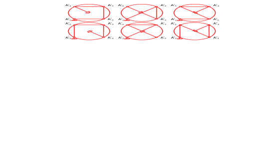
Figure 2.  : Six isotropic postures for the same isotropic set

and is apparently isotropic, with a triple singular value of $k=2$. We thus have $4!=24$ isotropic kinematic chains for a four-dof planar manipulator, but we represent only six in Fig. 2 because the choice of the first point is immaterial, since this choice amounts to a rotation of the overall manipulator as a rigid body. The conditioning length $l_{\cal P}$ is equal to $l/2$ for the three manipulators, with $l$ denoting any nonzero length. Moreover, the link lengths are defined, respectively, for three distinct manipulators of Fig. 2, form left to right: $a_{1}=l,a_{2}=l,a_{3}=l,a_{4}=\sqrt{2}l/2$; $a_{1}=l,a_{2}=\sqrt{2}l,a_{3}=l,a_{4}=\sqrt{2}l/2$; $a_{1}=\sqrt{2}l,a_{2}=l,a_{3}=\sqrt{2}l,a_{4}=\sqrt{2}l/2$.

An extensive discussion of isotropic sets of points and the optimum design of manipulators is available in (Chablat and Angeles, 1999.)

6 Conclusions

Isotropic manipulators are defined in this paper by resorting to the concept of isotropic sets of points. This concept allows us to define families of isotropic redundant manipulators. The characteristic length can thus be defined as the conditioning length $l_{\cal P}$ that pertains to the isotropic postures. The paper focuses on planar manipulators, but the underlying concepts are currently extended to their three-dimensional counterparts.

References

- Angeles (1997) Angeles, J., 1997, Fundamentals of Robotic Mechanical Systems, Springer-Verlag, New York.
- Angeles and Lopez-Cajun (1992) Angeles, J. and López-Cajún, C. S., 1992, “Kinematic Isotropy and the Conditioning Index of Serial Manipulators”, The Int. J. Robotics Research, Vol. 11, No. 6, pp. 560–571.
- Chablat and Angeles (1999) Chablat, D. and Angeles, J., 1999, On the Kinetostatic Optimization of Revolute-Coupled Planar Manipulators, Department of Mechanical Engineering and Centre for Intelligent Machines Technical Report, McGill University, Montreal.
- Golub and Van Loan (1997) Golub, G. H. and Van Loan, C. F., 1989, Matrix Computations, The John Hopkins University Press, Baltimore.
- Lee and Duffy and Hunt (1998) Lee, J., Duffy, J. and Hunt, K., 1998, “A Pratical Quality Index Based on the Octahedral Manipulator”, The International Journal of Robotic Research, Vol. 17, No. 10, October, pp. 1081–1090.
- Paden and Sastry (1988) Paden, B. and Sastry, S., 1988, “Optimal Kinematic Design of 6R Manipulator”, Int. Journal of Robotics Research, Vol. 7, No. 2, pp. 43–61.
- Ranjbaran and Angeles and Gonzales-Palacios (1995) Ranjbaran, F., Angeles, J., González-Palacios, M. A., and Patel, R. V., 1995, “The Mechanical Design of a Seven-Axes Manipulator with Kinematic Isotropy”, Journal of Intelligent and Robotic Systems, Vol. 14, pp. 21–41.
- Salisbury and Craig (1982) Salisbury, J. K. and Craig, J. J. 1982, “Articulated Hands: Force Control and Kinematic Issues”, Int. Journal of Robotic Research, Vol. 1, No. 1, pp. 4–17.