Transcritical bifurcations

in non-integrable Hamiltonian systems

Matthias Brack¹ and Kaori Tanaka^1,2

¹Institute for Theoretical Physics, University of Regensburg, D-93040 Regensburg, Germany

²Department of Physics and Engineering Physics, University of Saskatchewan,

Saskatoon, SK, Canada S7N 5E2

Abstract

We report on transcritical bifurcations of periodic orbits in non-integrable two-dimensional Hamiltonian systems. We discuss their existence criteria and some of their properties using a recent mathematical description of transcritical bifurcations in families of symplectic maps. We then present numerical examples of transcritical bifurcations in a class of generalized Hénon-Heiles Hamiltonians and illustrate their stabilities and unfoldings under various perturbations of the Hamiltonians. We demonstrate that for Hamiltonians containing straight-line librating orbits, the transcritical bifurcation of these orbits is the typical case which occurs also in the absence of any discrete symmetries, while their isochronous pitchfork bifurcation is an exception. We determine the normal forms of both types of bifurcations and derive the uniform approximation required to include transcritically bifurcating orbits in the semiclassical trace formula for the density of states of the quantum Hamiltonian. We compute the coarse-grained density of states in a specific example both semiclassically and quantum mechanically and find excellent agreement of the results.

1 Introduction

The transcritical bifurcation (TCB), in which a pair of stable and unstable fixed points of a map exchange their stabilities, is a well-known phenomenon in one-dimensional non-Hamiltonian systems. A simple example occurs in the quadratic logistic map (see, e.g., [2]):

$$x_{n+1}=r\,x_{n}(1-x_{n})\,,$$ (1)

where $\{x_{n}\}$ are arbitrary real numbers and $r$ is the control parameter. This map has – amongst others – two fixed points $x_{1}^{*}=0$ and $x_{2}^{*}=1-1/r$ which exchange their stabilities at the critical value $r=1$. For $r<1$, $x_{1}^{*}$ is stable and $x_{2}^{*}$ is unstable, whereas the inverse is true for $r>1$. [Note that in many textbooks discussing the quadratic map, this bifurcation is not mentioned as the values of the variable $x$ are usually confined to be non-negative, while $x_{2}^{*}<0$ for $r<1$.] The TCB occurs in many maps used to describe growth or population phenomena (see [3] for a recent example). TCBs have also been reported to occur in various time-dependent model systems [4, 5, 6, 7, 8, 9, 10] and shown, e.g., to be involved in synchronization mechanisms [6, 7]. In [9, 10], TCBs have been found to play a crucial role in transitions between low- and high-confinement states in confined plasmas, and their unfoldings have been analyzed.

To our knowledge, TCBs have not been discussed so far for periodic orbits in autonomous Hamiltonian systems. In this paper we report on the occurrence of such bifurcations in a class of two-dimensional non-integrable Hamiltonian systems. Since the TCB does not belong to the generic bifurcations in two-dimensional symplectic maps [11], we consider it useful to investigate also the mathematical conditions under which it can exist, its stability under perturbations of the Hamiltonian, and its unfoldings when it is destroyed by a perturbation. For this, we rely on mathematical studies by Jänich [12, 13] who introduced a class of “crossing bifurcations”, to which the TCB belongs, and derived several theorems and useful formulae for crossing bifurcations of straight-line librational orbits. Finally, in view of the important role which Gutzwiller’s semiclassical trace formula [14] plays for investigations of “quantum chaos” (see, e.g., [15, 16]), we study the inclusion of transcritically bifurcating orbits in the trace formula by an appropriate uniform approximation.

Generic bifurcations of fixed points in two-dimensional symplectic maps have been classified by Meyer [11] in terms of the number $m=1,2,\dots$ that corresponds to a period $m$-tupling occurring at the bifurcation. For an easily readable presentation of this classification of generic bifurcations, and of the corresponding normal forms used in semiclassical applications, we refer to the textbook of Ozorio de Almeida [17]. Bifurcations occurring in Hamiltonian systems with discrete symmetries have been investigated in [18, 19, 20, 21]; the TCB was, however, not mentioned in these papers. In [21] it has been shown that all other non-generic bifurcations occurring in such systems can be described by the generic normal forms given in [17], except for different bookkeeping of the number of fixed points which is connected not only to an $m$-tupling of the period, but also to degeneracies of the involved orbits due to the discrete symmetries. For the TCB this is not the case: it requires a normal form that is not in the generic list of [17]. We derive an appropriate normal form for the TCB, starting from the general criteria given in [12], and find it to correspond to that given in the literature for non-Hamiltonian systems [22, 23]. We use this normal form to develop the uniform approximation needed to include transcritically bifurcating orbits in the semiclassical trace formula. In a specific example that includes a TCB, we show numerically that our result allows to reproduce the coarse-grained quantum-mechanical density of states with a high precision.

In the nonlinear and semiclassical physics community, there exists an occasional belief that non-generic bifurcations occur only in systems which exhibit discrete symmetries (time-reversal symmetry being the most frequently met in physical systems). The examples of TCBs which we present in this paper are obtained in a class of autonomous Hamiltonian systems with mixed dynamics; starting from the famous Hénon-Heiles (HH) Hamiltonian [24] we change the coefficient of one of its cubic terms and add other terms destroying some or all of its discrete symmetries. All the TCBs that we have found involve one straight-line libration belonging to the shortest “period one” orbits. Our formal investigations therefore focus on the class of two-dimensional Hamiltonians containing a straight-line librational orbit. In this class of systems the TCB is, in fact, found to be the typical isochronous bifurcation of the librating orbit. The isochronous pitchfork bifurcation (PFB), however, which in Hamiltonian systems with time-reversal symmetry (such as the standard HH system) is the most frequently met non-generic bifurcation, is the exception here. We show how under a specific perturbation the PFB can unfold into a saddle-node bifurcation (SNB) followed by a TCB. In a specific example, we demonstrate that the TCB can exist in a system without any discrete (spatial or time-reversal) symmetry, thus proving that the above-mentioned belief is incorrect.

Our paper is organized as follows. In Sec. 2 we compile results of Jänich [12, 13] relevant for our investigations. Starting from two-dimensional symplectic maps, we define a class of “crossing bifurcations” to which the TCB and the isochronous PFB belong. We discuss various criteria and properties of these bifurcations and give some useful formulae for the specific case of a bifurcating straight-line libration. The mathematically less interested reader may skip Sec. 2 and jump directly to Sec. 3, where we present numerical examples of the TCB and their characteristic features in the generalized Hénon-Heiles Hamiltonians. We also study there various types of unfoldings of the TCB under perturbations of the Hamiltonian. In Sec. 4 we discuss the semiclassical trace formula for the density of states of a quantum Hamiltonian, and present the uniform approximation by which bifurcating periodic orbits can be included. In Sec. 4.4 we present a semiclassical calculation of the density of states in a situation where the TCB occurs between two of the shortest periodic orbits, and demonstrate the validity of the uniform approximation by comparison of the results with those of a fully quantum-mechanical calculation. In App. 6 we derive the appropriate normal forms for the TCB and the isochronous PFB which are needed in semiclassical applications. In App. 7 we briefly discuss the stability exchange of two orbits in a “false transcritical bifurcation” which actually consists of a pair of close-lying pitchfork bifurcations.

2 Mathematical prerequisites

In this section we present results of Jänich [12, 13] which are relevant for our investigations. We shall only quote theorems and other results; for readers interested in the mathematical proofs or other details, we refer to the explicit contents of [12, 13].

2.1 Poincaré map and stability matrix

We are investigating bifurcations of periodic orbits in two-dimensional Hamiltonian systems. They are most conveniently investigated and mathematically described by observing the fixed points on a suitably chosen projected Poincaré surface of section (PSS). Since the PSS here is two-dimensional, we describe it by a pair of canonical variables $(q,p)$. The time evolution of an orbit then corresponds to the two-dimensional Poincaré map

$$(q,p)\longrightarrow(Q,P)\,,$$ (2)

where $(q,p)$ is the initial and $(Q,P)$ the final point on the PSS. Fixed points of this map, defined by $Q=q$, $P=p$, correspond to periodic orbits. We introduce $\epsilon$ as a “bifurcation parameter” which in principle may be the conserved energy of the system or any potential parameter, normalized such that a bifurcation occurs at $\epsilon=0$. Here we specialize to the energy variable by defining

$$\epsilon=E-E_{0}\,,$$ (3)

where $E_{0}$ is the energy at which the considered bifurcation takes place. We assume that the bifurcating orbit returns to the same point on the PSS after one map (2), so that $Q=q$, $P=p$; in this paper this will be called a “period one” orbit. We shall only study its isochronous bifurcations and hence only consider the non-iterated Poincaré map.

The map (2) is symplectic and thus area conserving in the $(q,p)$ plane, and may be understood as a canonical transformation:

$$Q=Q(q,p,\epsilon)\,,\qquad P=P(q,p,\epsilon)\,.$$ (4)

Jänich [12] has given a classification of bifurcations of fixed points in two-dimensional symplectic maps, which we shall summarize in the following. We use his notation $Q_{u}$, $P_{u}$ for partial derivatives of the functions $Q$ and $P$, respectively, with respect to $u$:

$$Q_{u}=\frac{{\partial Q}}{{\partial u}}\,,\qquad P_{u}=\frac{{\partial P}}{{\partial u}}\,,$$ (5)

where $u$ is any of the three variables $q,p$ or $\epsilon$. Analogously $Q_{qq}$, $P_{qp\epsilon}$, etc., denote second and higher partial derivatives. Due to the symplectic nature of (4), the determinant of the first derivatives of $Q$ and $P$ with respect to $q$ and $p$ is unity:

$${\rm det}\left(\begin{array}[]{cc}Q_{q}(q,p,\epsilon)&Q_{p}(q,p,\epsilon)\\ P_{q}(q,p,\epsilon)&P_{p}(q,p,\epsilon)\end{array}\right)=1\,.$$ (6)

We consider an isolated “period one” orbit with fixed point $(q,p)=(0,0)$, for all values of $\epsilon$ where it exists, and denote it as the A orbit. Its stability matrix is then given by

$${\rm M}_{\rm A}(\epsilon)=\left(\begin{array}[]{cc}Q_{q}(0,0,\epsilon)&Q_{p}(0,0,\epsilon)\\ P_{q}(0,0,\epsilon)&P_{p}(0,0,\epsilon)\end{array}\right).$$ (7)

At $\epsilon=0$, where the orbit undergoes an isochronous bifurcation, ${\rm M}_{\rm A}(0)$ has two degenerate eigenvalues +1, so that ${\rm tr}\,{\rm M}_{\rm A}(0)=2$.

Henceforth we shall omit the arguments (0,0,0) in the partial derivatives of $Q$ and $P$ which – unless explicitly mentioned otherwise – will always be evaluated at the bifurcation point. When we need some of these partial derivatives at $p=q=0$ but at arbitrary values of $\epsilon$, we shall denote them by $Q_{p}(\epsilon)$ etc. When no argument is given, $\epsilon=0$ is assumed. We thus write

$${\rm M}_{\rm A}(\epsilon)=\left(\begin{array}[]{cc}Q_{q}(\epsilon)&Q_{p}(\epsilon)\\ P_{q}(\epsilon)&P_{p}(\epsilon)\end{array}\right),\qquad{\rm M}_{\rm A}(0)=\left(\begin{array}[]{cc}Q_{q}&Q_{p}\\ P_{q}&P_{p}\end{array}\right).$$ (8)

The slope of the function ${\rm tr}\,{\rm M}_{\rm A}(\epsilon)$ at $\epsilon=0$ (coming from a side where the orbit A exists) becomes, in this notation,

$${\rm tr}\,{\rm M}_{\rm A}^{\prime}(0)=Q_{q\epsilon}+P_{p\epsilon}\,.$$ (9)

By a rotation of the canonical coordinates $q,p$ it is always possible to bring ${\rm M}_{\rm A}(0)$ into the form:

$${\rm M}_{\rm A}(0)=\left(\begin{array}[]{cc}1&Q_{p}\\ 0&1\end{array}\right),\qquad Q_{p}\neq 0\,.$$ (10)

We shall henceforth assume that the coordinates have been chosen such that (10) is true. Then, with (6) one finds easily the determinant derivative formula [12]

$$Q_{qu}+P_{pu}=Q_{p}P_{qu}\quad\qquad(u=q,p,\epsilon)\,,$$ (11)

and (9) takes the simpler form

$${\rm tr}\,{\rm M}_{\rm A}^{\prime}(0)=Q_{p}P_{q\epsilon}\,.$$ (12)

The total fixed point set

$$F:=\{(q,p,\epsilon)\,|\,Q(q,p,\epsilon)=q,\,P(q,p,\epsilon)=p\}$$ (13)

is the inverse image of the origin $(0,0)$ in $\mathbb{R}^{2}$ under the map $(Q-q,P-p)$ whose Jacobian matrix at $(0,0,0)$ is

$${\rm J}=\left(\begin{array}[]{ccc}Q_{q}-1&Q_{p}&Q_{\epsilon}\\ P_{q}&P_{p}-1&P_{\epsilon}\\ \end{array}\right)=\left(\begin{array}[]{ccc}0&Q_{p}&Q_{\epsilon}\\ 0&0&P_{\epsilon}\\ \end{array}\right).$$ (14)

In the generic case, $P_{\epsilon}\neq 0$ and J has rank 2. This leads to the only generic isochronous bifurcation according to Meyer [11], the saddle-node bifurcation (SNB) (also called “tangent bifurcation”). For this bifurcation, the fixed-point set $F$ (13) is a smooth one-dimensional manifold, consisting of two half-branches tangent to the $q$ axis at the bifurcation point with slopes ${\rm tr}\,{\rm M}_{\rm A}^{\prime}(0)=\pm\infty$. The orbit A then exists either only for $\epsilon\leq 0$ or only for $\epsilon\geq 0$; no other orbit takes part in such a bifurcation.

Following Jänich [12], we speak of a rank 1 bifurcation, when the Jacobian J in (14) has rank 1, which is the case for

$$P_{\epsilon}=0\,.$$ (15)

Then, after a suitable ($\epsilon$-dependent) translation of the $p$ variable, J can always be brought into the form

$${\rm J}=\left(\begin{array}[]{ccc}Q_{q}-1&Q_{p}&Q_{\epsilon}\\ P_{q}&P_{p}-1&P_{\epsilon}\\ \end{array}\right)=\left(\begin{array}[]{ccc}0&Q_{p}&0\\ 0&0&0\\ \end{array}\right).$$ (16)

We shall formulate all following developments in the suitably adapted coordinates $(q,p)$, for which the form (16) holds, and discuss only rank 1 bifurcations.

2.2 Crossing bifurcations of isolated periodic orbits

A rank 1 bifurcation for which the Hessian

$${\rm K}=\left(\begin{array}[]{cc}P_{qq}&P_{q\epsilon}\\ P_{q\epsilon}&P_{\epsilon\epsilon}\end{array}\right)$$ (17)

at (0,0,0) is regular and indefinite, i.e., for which det K $=P_{qq}P_{\epsilon\epsilon}-P_{q\epsilon}^{2}<0$, shall be called a crossing bifurcation. Jänich showed [12] that a necessary and sufficient criterion for an orbit A to undergo a crossing bifurcation at $\epsilon=0$ is for the slope ${\rm tr}\,{\rm M}_{\rm A}^{\prime}(\epsilon=0)$ to be finite and nonzero. With (10) and (12) we see that

$$P_{q\epsilon}\neq 0\,$$ (18)

for crossing bifurcations. It follows that if the orbit A undergoes a crossing bifurcation at $\epsilon=0$, it exists on both sides of a finite two-sided neighborhood of $\epsilon=0$. Jänich also showed that for such a bifurcation, the total fixed-point set $F$ (13) is the union $A\cup B$ of two smooth 1-dimensional submanifolds intersecting at the bifurcation point. The set $A$ is the set of fixed points $(0,0,\epsilon)$ of the A orbit; we shall call it the fixed-point branch $A$. The set $B$ is the fixed-point set of a second orbit B which takes part in the crossing bifurcation.

We shall discuss here only two types of crossing bifurcations: transcritical and fork-like bifurcations. Their properties are specified in the following two subsections. A rank 1 bifurcation with a regular and definite Hessian K, i.e., with det K $>0$, is sometimes called an “isola center” (cf. the normal form for the isola center in one-dimensional Hamiltonians at the end of Sec. 6.1). Here the total fixed-point set F consists of the single isolated point $(q,p,\epsilon)=(0,0,0)$.

2.2.1 Transcritical bifurcation (TCB)

A transcritical bifurcation (TCB) occurs when, in the adapted coordinates $(q,p)$ for which (10) holds, one has

$$P_{qq}\neq 0\,.$$ (19)

Then, there exists another isolated periodic orbit B on both sides of $\epsilon=0$, forming a fixed-point branch $B$ intersecting that of the orbit A at $\epsilon=0$ with a finite angle. The functions ${\rm tr}\,{\rm M}_{\rm A}(\epsilon)$ and ${\rm tr\,M}_{\rm B}(\epsilon)$ have opposite slopes at the bifurcation:

$${\rm tr}\,{\rm M}_{\rm A}^{\prime}(0)=-\,{\rm tr\,M}^{\prime}_{\rm B}(0)\,.\qquad(\hbox{\it``TCB~{}slope~{}theorem''})$$ (20)

In the scenario of a TCB, the orbits A and B simply exchange their stabilities and no new orbit appears (or no old orbit disappears) at the bifurcation.

Note: Assume that the orbit A is a straight-line libration, chosen to lie on the $y$ axis, so that the Poincaré variables are $q=x$, $p=p_{x}$ (see Sec. 2.3 below). Then, if the system is invariant under reflexion at the $y$ axis, such a reflexion leads to $P(q,p,\epsilon)=-P(-q,-p,\epsilon)$. Therefore, $P_{qq}(q=0,p=0,\epsilon=0)=P_{qq}=0$, and the bifurcation cannot be transcritical. The simplest possible crossing bifurcation then is fork-like (see next item). In short: Straight-line librations along symmetry axes cannot undergo transcritical bifurcations.

2.2.2 Fork-like bifurcation (FLB)

A fork-like bifurcation (FLB) occurs when one has

$$P_{qq}=0\,,\qquad P_{qqq}\neq 0\,.$$ (21)

Then, there exists another isolated periodic orbit B, either only for $\epsilon\geq 0$ or only for $\epsilon\leq 0$. The fixed-point set of B consists of two half-branches intersecting the set $A$ at $\epsilon=0$ at a right angle. In the adapted coordinates corresponding to (10), one may parameterize the set $B$ by $(q,p_{B}(q),\epsilon_{B}(q))$ and finds

$$p^{\prime}_{B}(0)=\epsilon^{\prime}_{B}(0)=0\,,\qquad\epsilon^{\prime\prime}_{B}(0)\neq 0\,.$$ (22)

Although ${\rm tr\,M}_{\rm B}(\epsilon)$ is not a proper function of $\epsilon$, a limiting slope ${\rm tr\,M}^{\prime}_{\rm B}(0)\neq 0$ can be defined for both half-branches of the set $B$ in the limit $\epsilon\to 0$, coming from that side where they exist, and be shown [12] to fulfill the relation

$${\rm tr\,M}^{\prime}_{\rm B}(0)=-2\,{\rm tr}\,{\rm M}_{\rm A}^{\prime}(0)\,.\qquad(\hbox{\it``FLB~{}slope~{}theorem''})$$ (23)

In the same limit, the curvature of the set $B$ at the bifurcation point is given by

$$\epsilon^{\prime\prime}_{B}(0)=\frac{3Q_{qq}P_{qp}-Q_{p}P_{qqq}}{3Q_{p}P_{q\epsilon}}\,.$$ (24)

In the pertinent physics literature, this bifurcation is often called the (non-generic) isochronous pitchfork bifurcation (PFB). Note that here the two half-branches of the set $B$ correspond to two different periodic orbits. They can be either locally degenerate (to first order in $\epsilon$), or globally degenerate due to a discrete symmetry (reflexion at a symmetry axis or time reversal).

In the generic PFB corresponding to Meyer’s classification [11], the fixed point scenario near $\epsilon=0$ is identical with that of the FLB. However, here the two fixed points of the set $B$ correspond to one single orbit B which has twice the period of the primitive orbit A. In fact, the fixed-point branch $A$ crossing the line ${\rm tr}\,{\rm M}_{\rm A}=2$ is that of the iterated Poincaré map: the generic PFB is period doubling. The existence criterion (21) and the relations (22) - (24) for the B orbit hold here, too [26].

2.3 Some explicit formulae for straight-line librations

2.3.1 Definition of the librational A orbit

We now specialize to straight-line librational orbits in two-dimensional autonomous Hamiltonian systems, defined by Hamiltonian functions

$$H_{0}(x,y,p_{x},p_{y})=\frac{1}{2}\,(p_{x}^{2}+p_{y}^{2})+V(x,y)$$ (25)

with a smooth potential $V(x,y)$. Straight-line librations form the simplest type (and so far the only one known to us) of periodic orbits in Hamiltonian systems that undergo transcritical bifurcations. Let us choose the direction of the libration to be the $y$ axis and call it the A orbit. The potential then must have the property

$$\frac{\partial V}{\partial x}\,(0,y)=0$$ (26)

for all $y$ reached by the libration. The A orbit, which we assume to be bound at all energies, then has $x(t)={\dot{x}}(t)=0$ for all times $t$, and its $y$ motion is given by the Newton equation

$${\ddot{y}}(t)+\frac{\partial V}{\partial y}\,(0,y(t))=0\qquad\Rightarrow\qquad y(t)=y_{A}(t,\epsilon)\,,$$ (27)

where $y_{A}(t,\epsilon)$ is henceforth assumed to be a known periodic function of $t$ with period $T_{A}(\epsilon)$. For the A orbits in the (generalized) HH potentials discussed in the following section, the function $y_{A}(t,\epsilon)$ can be expressed in terms of a Jacobi-elliptic function [27]. We choose the time scale such that $y_{A}(0,\epsilon)$ is maximum with

$${\dot{y}}_{A}(0,\epsilon)=0\qquad\forall\;\epsilon\,.$$ (28)

A suitable choice of Poincaré variables is to use the surface of section defined by $y=0$, and the projected PSS becomes the $(x,p_{x})$ plane, so that we define $q=x$, $p=p_{x}$. We again assume that the orbit A is isolated and exists in a finite interval of $\epsilon$ around zero. The fixed-point branch $A$ is thus again given by the straight line $(q_{A},p_{A},\epsilon)=(0,0,\epsilon)$ in the $(q,p,\epsilon)$ space.

In [13] Jänich has given an iterative scheme to calculate the partial derivatives $Q_{q}$, $Q_{p}$, etc. for this situation for any given (analytical) potential $V(x,y)$ with the above properties. To this purpose, one has first to determine the fundamental systems of solutions $(\xi_{1},\xi_{2})$ and $(\eta_{1},\eta_{2})$ of the linearized equations of motion in the $x$ and $y$ directions, respectively:

$${\ddot{\xi}}(t)+V_{xx}(0,y_{A}(t,\epsilon))\,\xi(t) = 0\,,$$ (29)

$${\ddot{\eta}}(t)+V_{yy}(0,y_{A}(t,\epsilon))\,\eta(t) = 0\,,$$ (30)

with the initial conditions

$$\left(\begin{array}[]{cc}\xi_{1}(0)&\xi_{2}(0)\\ {\dot{\xi}}_{1}(0)&{\dot{\xi}}_{2}(0)\end{array}\right)=\left(\begin{array}[]{cc}\eta_{1}(0)&\eta_{2}(0)\\ {\dot{\eta}}_{1}(0)&{\dot{\eta}}_{2}(0)\end{array}\right)=\left(\begin{array}[]{cc}1&0\\ 0&1\end{array}\right)\qquad\forall\;\epsilon.$$ (31)

For simplicity, we do not give the argument $\epsilon$ of the $\xi_{i}(t)$ and $\eta_{i}(t)$, but we should keep in mind that they are all functions of $\epsilon$. In (29), (30) the subscripts on the function $V(x,y)$ denote its second partial derivatives with respect to the corresponding coordinates. In the formulae given below, we denote by $V_{i}(t)$, $V_{ij}(t)$, etc., with $i,j\in(x,y)$ the partial derivatives taken along the A orbit, i.e., at $x=0$, $y=y_{A}(t,\epsilon)$ as in (29), (30), evaluated at the bifurcation point $\epsilon=0$. If the partial derivatives have no argument, they are taken at the period $T_{A}(\epsilon_{0})$, i.e., $V_{y}=V_{y}(T_{A}(\epsilon_{0}))$ etc.

Knowing the five functions $y_{A}(t,\epsilon=0)$ and $\xi_{i}(t),\eta_{i}(t)$ $(i=1,2)$ at $\epsilon=0$, all desired partial derivatives of $Q(q,p,\epsilon)$ and $P(q,p,\epsilon)$ at $(q,p,\epsilon)=(0,0,0)$ can be obtained by (progressively repeated) quadratures, i.e., by finite integrals over known expressions including these five functions, partial derivatives of $V(x,y)$, and the functions obtained at earlier steps of the scheme (whereby the progression comes from increasing degrees of the desired partial derivatives).

2.3.2 Stability matrix of the A orbit

We note that the equation (29) is nothing but the stability equation of the A orbit, since the $\xi_{i}$ by definition are small variations transverse to the orbit. In the standard literature, (29) is also called the “Hill equation” (cf., e.g., [15, 28]). The stability matrix ${\rm M}_{\rm A}$ at the bifurcation of the A orbit is therefore simply given by

$${\rm M}_{\rm A}(0)=\left(\begin{array}[]{cc}Q_{q}&Q_{p}\\ P_{q}&P_{p}\end{array}\right)=\left(\begin{array}[]{cc}\xi_{1}(T_{A})&\xi_{2}(T_{A})\\ {\dot{\xi}}_{1}(T_{A})&{\dot{\xi}}_{2}(T_{A})\end{array}\right),$$ (32)

with $T_{A}=T_{A}(\epsilon=0)$. Its eigenvalues must be $\lambda_{1}=\lambda_{2}=+1$, as seen directly from (10). The solutions $\xi_{i}(t,\epsilon)$ of (29) are in general not periodic. But at the bifurcations of the A orbit, where ${\rm tr\,M}_{A}=+2$, one of the $\xi_{i}(t,\epsilon=0)$ is always periodic with period $T_{A}$ (or an integer multiple $m$ thereof) [28] and describes, up to a normalization constant depending on $\epsilon$, the transverse motion of the bifurcated orbit at an infinitesimal distance $\epsilon$ from the bifurcation (cf. [27, 29, 30]).

2.3.3 Slope of the function ${\rm tr}\,{\rm M}_{\rm A}(\epsilon)$ at $\epsilon=0$

Here we give the explicit formulae, obtained from [13], for the slope ${\rm tr}\,{\rm M}_{\rm A}^{\prime}(0)=Q_{q\epsilon}+P_{p\epsilon}$, see (9), of the function ${\rm tr}\,{\rm M}_{\rm A}(\epsilon)$ at the bifurcation. The quantities $Q_{q\epsilon}$ and $P_{p\epsilon}$ are given, in terms of the potential $V(x,y)$ in (25) and the other ingredients defined above, by

$$Q_{q\epsilon} = \;\frac{1}{(V_{y})^{2}}\,P_{q}\,{\dot{\eta}}_{1}(T_{A})-\frac{1}{V_{y}}\int_{0}^{T_{A}}V_{xxy}(t)\left[Q_{p}\,\xi_{1}(t)-Q_{q}\,\xi_{2}(t)\right]\xi_{1}(t)\,\eta_{1}(t)\,{\rm d}t\,,$$ (33)

$$P_{p\epsilon} = \frac{(-V_{xx})}{(V_{y})^{2}}\,Q_{p}\,{\dot{\eta}}_{1}(T_{A})-\frac{1}{V_{y}}\int_{0}^{T_{A}}\!V_{xxy}(t)\left[P_{p}\,\xi_{1}(t)-P_{q}\,\xi_{2}(t)\right]\xi_{2}(t)\,\eta_{1}(t)\,{\rm d}t\,.$$ (34)

In the adapted coordinates where ${\rm tr}\,{\rm M}_{\rm A}(0)$ has the form (10) with $Q_{q}=P_{p}=1$ and $P_{q}=0$, the slope becomes

$${\rm tr}\,{\rm M}_{\rm A}^{\prime}(0)=Q_{p}\,P_{q\epsilon}=\frac{(-V_{xx})}{(V_{y})^{2}}\,Q_{p}\,{\dot{\eta}}_{1}(T_{A})-\frac{1}{V_{y}}\,Q_{p}\int_{0}^{T_{A}}V_{xxy}(t)\,\xi_{1}^{2}(t)\,\eta_{1}(t)\,{\rm d}t\,.$$ (35)

For the case that ${\rm tr}\,{\rm M}_{\rm A}(0)$ has the transposed tridiagonal form with $Q_{p}=0$ and $P_{q}\neq 0$, the formula becomes

$${\rm tr}\,{\rm M}_{\rm A}^{\prime}(0)=P_{q}\,Q_{p\epsilon}=\frac{1}{(V_{y})^{2}}\,P_{q}\,{\dot{\eta}}_{1}(T_{A})+\frac{1}{V_{y}}\,P_{q}\int_{0}^{T_{A}}V_{xxy}(t)\,\xi_{2}^{2}(t)\,\eta_{1}(t)\,{\rm d}t\,.$$ (36)

An independent derivation of (33) - (36) is given in [31], where it is shown that the first terms are due to the variation of the A orbit’s period $T_{A}$ with $\epsilon$, whereas the integral terms are due to the $\epsilon$ dependence of the functions $\xi_{i}(t)$.

2.3.4 Criterion for the TCB

For a bifurcation to be transcritical, we need $P_{qq}\neq 0$. From [13] we find the following explicit formula for $P_{qq}$

$$P_{qq}=-\int_{0}^{T_{A}}V_{xxx}(t)\,\xi_{1}^{3}(t)\,{\rm d}t\,,$$ (37)

which also yields explicitly the parameter $b$ in its normal form given in (96) below.

If the potential is symmetric about the $y$ axis, then $V_{xxx}(t)$ is identically zero and the TCB cannot occur, as already stated in Sec. 2.2.1 above. However, even if $V_{xxx}(t)$ is not zero, special symmetries of the function $\xi_{1}(t)$, in combination with that of $V_{xxx}(t)$, can make the integral in (37) vanish. An example of this is discussed in Sec. 3.3.5.

3 TCBs in the generalized Hénon-Heiles potential

3.1 The generalized Hénon-Heiles potential

For our numerical studies, we have investigated the following family of generalized Hénon-Heiles (GHH) Hamiltonians:

$$H(x,y,p_{x},p_{y})=\frac{1}{2}\,(p_{x}^{2}+p_{y}^{2})+\frac{1}{2}\,(x^{2}+y^{2})+\alpha\left[-\frac{1}{3}\,y^{3}+\gamma\,x^{2}y+\beta\,y^{2}x\right].$$ (38)

Here $\alpha$ is the control parameter that regulates the nonlinearity of the system, and $\gamma$, $\beta$ are parameters that define various members of the family. The standard HH potential [24] corresponds to $\gamma=1$, $\beta=0$. It has three types of discrete symmetries: ($i$) rotations about $2\pi/3$ and $4\pi/3$, and ($ii$) reflections at three corresponding symmetry lines, which together define the C_3v symmetry, and ($iii$) time-reversal symmetry. There exist three saddles at the critical energy $E^{*}=1/6\alpha^{2}$, so that the system is unbound and a particle can escape if its energy is $E>E^{*}$. For $\gamma\neq 1$, $\beta\neq 0$, the spatial symmetries are in general broken (except for particular values of $\gamma$ and $\beta$) and only the time-reversal symmetry is left. There still exist three saddles, but in general they lie at different energies. There is always a stable minimum at $x=y=0$.

It is convenient to scale away the nonlinearity parameter $\alpha$ in (38) by introducing scaled variables $x^{\prime}=\alpha x$, $y^{\prime}=\alpha y$ and a scaled energy $e=E/E^{*}=6\alpha^{2}E$. Then (38) becomes

$$h=e=6\alpha^{2}E=3\,(p_{x^{\prime}}^{2}+p_{y^{\prime}}^{2}+x^{\prime 2}+y^{\prime 2})-2\,y^{\prime 3}+6\,(\gamma\,x^{\prime 2}y^{\prime}+\beta\,y^{\prime 2}x^{\prime})\,,$$ (39)

so that one has to vary one parameter less to discuss the classical dynamics. (For the standard HH potential with $\gamma=1$, $\beta=0$, the scaled energy $e$ then is the only parameter.) For simplicity, we omit henceforth the primes of the scaled variables $x^{\prime},y^{\prime}$.

Before we discuss the periodic orbits in the system (39), let us briefly recall the situation in the standard HH system in which all three saddles lie at the scaled energy $e=1$.

3.1.1 Periodic orbits in the standard HH potential

The periodic orbits of the standard HH system have been studied in [27, 29, 32, 33], and their use in connection with semiclassical trace formulae in [34, 35, 36, 37, 38, 39]. We also refer to [25] (section 5.6.4) for a short introduction into this system, which represents a paradigm of a mixed Hamiltonian system covering the transition from integrability ($e=0$) to near-chaos ($e>1$).

In Fig. 1 we show the trace tr M of the stability matrix M, henceforth called “stability trace”, of the shortest orbits as a function of $e$. Up to energy $e\simeq 0.97$, there exist [32] only three types of “period one” orbits [in the sense defined after (3)]: 1) straight-line librations A along the three symmetry axes, oscillating towards the saddles; 2) curved librations B which intersect the symmetry lines at right angles and are hyperbolically unstable at all energies; and 3) rotational orbits C in the two time-reversed versions which are stable up to $e\simeq 0.89$ and then become inverse-hyperbolically unstable. While the B and C orbits exist at all energies, the orbits A cease to exist at the critical saddle energy $e=1$ where their period becomes infinite.

When $|$tr M$|>$ 2 or $<$ 2, an orbit is unstable or stable, respectively. When tr M = 2 it either undergoes a bifurcation if the orbit is isolated, or it belongs to a family of degenerate orbits in the presence of a continuous symmetry. The latter is seen to occur in the limit $e\rightarrow 0$, where the orbits A, B and C all converge to the family of orbits of the isotropic two-dimensional harmonic oscillator with U(2) symmetry. The A orbits undergo an infinite sequence of (non-generic) isochronous PFBs, starting at $e\simeq 0.97$ and cumulating at $e=1$. At these bifurcations an alternating sequence of rotational orbits (labeled R) and librational orbits (labeled L) are born. This bifurcation cascade, the R and L type orbits, and their self-similarity have been discussed extensively in [27, 29]. In Fig. 1 and in the text below, we indicate their Maslov indices (needed in semiclassical trace formulae, see Sec. 4) by suffixes to their labels, which allows for unique bookkeeping of all orbits. (Only the first two representatives R₅ and L₆ of the orbits born along the bifurcation cascade are shown in Fig. 1 by the dashed lines.) At each bifurcation, the orbit A increases its Maslov index (which is 5 up to the first bifurcation) by one unit. Only the first three bifurcations can be seen in the figure; the others are all compressed into a tiny interval below $e=1$. As has been observed numerically in [27, 29, 33], tr M_A becomes a periodic function of the period $T_{A}$ in the limit $e\rightarrow 1$. [It can actually be rigorously shown that, asymptotically, tr M${}_{A}(T_{A})\longrightarrow-2.68042\,\sin(\sqrt{3}\,T_{A})$ in this limit [31].]

Figure 1: Trace of the stability matrix M of the “period one” orbits in the standard HH potential, plotted versus scaled energy $e$. The suffixes indicate their Maslov indices. Only the first two (R₅ and L₆) of the orbits born at an infinite sequence of isochronous PFBs of the A orbit, cumulating at the saddle energy $e=1$, are shown (dashed lines).

As is characteristic of isochronous PFBs (cf. Sec. 2.2.2), the new-born orbits come in degenerate pairs due to the discrete symmetries: the two librational L orbits are mapped onto each other under reflection at the axis containing the A orbit, and the two rotational R orbits are connected by time reversal. Note that although the A orbit ceases to exist for $e\geq 1$, all R and L type orbits bifurcated from it exist at all energies $e\geq 1$. For some new orbits appearing there, we refer to the literature [33, 39]; in this paper we shall not be concerned with them.

3.1.2 Periodic orbits in the generalized HH potential

For $\gamma\neq 0$, $\beta\neq 0$, there exist in general three different saddles at scaled energies $e_{0}$, $e_{1}$ and $e_{2}$, and three different straight-line periodic orbits, labeled A, A’ and A”, oscillating towards the saddles. In general, there are three curved librational orbits B, B’ and B” (not necessarily existing at all energies) intersecting the three A type orbits at right angles, and there is always a time-reversally degenerate pair of rotational orbits C going around the origin. It is rather easy to see that the three A type orbits always intersect each other at the minimum of the potential located at the origin $(x,y)=(0,0)$. The equations of motion for the Hamiltonian (38) in the Newton form are (in the scaled variables corresponding to $\alpha=1$)

$$\ddot{x}+x\,(1+2\gamma\,y)+\beta\,y^{2} = 0\,,$$

$$\ddot{y}+y\,(1+2\beta\,x)+\gamma\,x^{2}-y^{2} = 0\,.$$ (40)

For a straight-line orbit librating through the origin we have $y=ax$ which, inserted into (40), yields a cubic equation for the slope $a$:

$$\beta\,a^{3}+(2\gamma+1)\,a^{2}-2\beta\,a-\gamma=0\,.$$ (41)

For the rest of this paper, we limit the parameters to the range $\gamma>0$ and $\beta\geq 0$. Then, (41) has always real roots that are in general different. In the right panel of Fig. 2 below, we have shown the six shortest (“period one”) librations obtained numerically for $\gamma=0.6$, $\beta=0.07$, including the three straight-line orbits A, A’, A” intersecting at the origin.

Further analytical analysis is cumbersome except for the following special cases:

$\beta=0$, $\gamma=1$ (standard HH) :
Two of the slopes are $a_{1,2}=\pm 1/\!\sqrt{3}$; the third is $a_{0}=\infty$ corresponding to the orbit along the $y$ axis with $x(t)=0$. The three saddles lie at $(x,y)=(0,1)$, $(-\sqrt{3}/2,-1/2)$, and $(\sqrt{3}/2,-1/2)$, forming an equilateral triangle with side length $\sqrt{3}\,$; its sides (and their extensions) form the equipotential lines for $e=1$. The periodic orbits are those discussed in Sec. 3.1.1.

$\beta=0$, $\gamma\neq 1$:
The rotational $C_{3v}$ symmetry is broken, but the reflection symmetry at the $y$ axis is kept. Correspondingly, we find two degenerate orbits A’, A” with opposite slopes $a_{1,2}=\pm\sqrt{\gamma/(2\gamma+1)}$. There is a horizontal equipotential line at $y_{1}=y_{2}=-1/2\gamma$ with scaled energy $e_{1}=e_{2}=(3+1/\gamma)/4\gamma^{2}$ that contains two saddle points symmetrically positioned at $x_{1,2}=\pm\sqrt{(2+1/\gamma)}/2\gamma$. At low energies, there is only one B type orbit intersecting the $y$ axis at a right angle; two further orbits B’ and B” appear through bifurcations at higher energies (see examples in Sec. 3.2). For $\gamma>0$ there is a third A orbit librating along the $y$ axis ($a_{0}=\infty$) towards a third saddle at $(0,1)$ with energy $e_{0}=1$. The equipotential line for $e=e_{1,2}$ consists of the horizontal line at $y_{1,2}=-1/2\gamma$ and two branches of a hyperbola. For $\gamma>1$ the hyperbola branches lie symmetrically about the $y$ axis, each intersecting the horizontal line at one of the two symmetric saddle points. For $0<\gamma<1$, they lie symmetrically about a horizontal line at $y^{*}=(1+3\gamma)/4\gamma$, the lower of them intersecting the line $y=y_{1,2}$ at the two symmetric saddle points.

The limiting case $\beta=0$, $\gamma=0$ yields a separable and hence integrable system with only one saddle at $(0,1)$ at energy $e_{0}=1$ and one A orbit (with $a=\infty$). We do not discuss this system here, but refer to [38] in which it is investigated both classically and semiclassically in full detail.

3.2 Examples of transcritical bifurcations and their properties

As mentioned above, we have restricted the parameters $\gamma$ and $\beta$ in the GHH potential (38) to be positive (or $\beta=0$). We find that, depending on the values of $\beta$ and $\gamma$, at least one or two of the straight-line orbits A, A’, or A” can undergo a TCB with a partner of the curved librational orbits B, B’, or B”. In the following, we shall first show two examples and then discuss characteristic properties of the TCB. In Sec. 3.3 we shall study its stability and its unfoldings. Some of the numerical results can easily be understood analytically in terms of the normal forms of the various bifurcations and their unfoldings. These are discussed in detail in App. 6 and shall be referred to in the following text.

3.2.1 Two examples

As a numerical example, we choose $\gamma=0.6$, $\beta=0.07$. The three saddle energies are e${}_{0}=0.993$ for the A orbit, $e_{1}=2.81$ for the A’ orbit, and $e_{3}=3.74$ for the A” orbit. In the left panel of Fig. 2 we show the stability traces tr M($e$) of the shortest orbits. In the right panel we display the shapes of these orbits in the $(x,y)$ plane. The orbits B’ and B” are created in a SNB at $e_{tb}\simeq 1.533$ and do not exist below this energy; at high energies they are hyperbolically unstable with increasing Lyapunov exponents. Contrary to the standard HH system, only the A orbit is stable at low energies, while the orbits A’ and A” leave the $e=0$ limit unstable and cross the critical line tr M = +2 at some finite energies $e_{tcb}$ and $e^{\prime}_{tcb}$ to become stable. At higher energies, all three A type orbits undergo an infinite PFB cascade as in Fig. 1, each of them converging at its saddle energy. (We do not show here the R and L type orbits born at these bifurcations.)

It is between the pairs of orbits A’, B and A”, B’ that we here observe two TCBs. They occur at the energy $e_{tcb}=0.854447$ between the orbits A’ and B, and at $e^{\prime}_{tcb}=1.644$ between the orbits A” and B’. The situation near $e^{\prime}_{tcb}$ actually displays an example of a slightly broken PFB which will be discussed in Sec. 3.3.5.

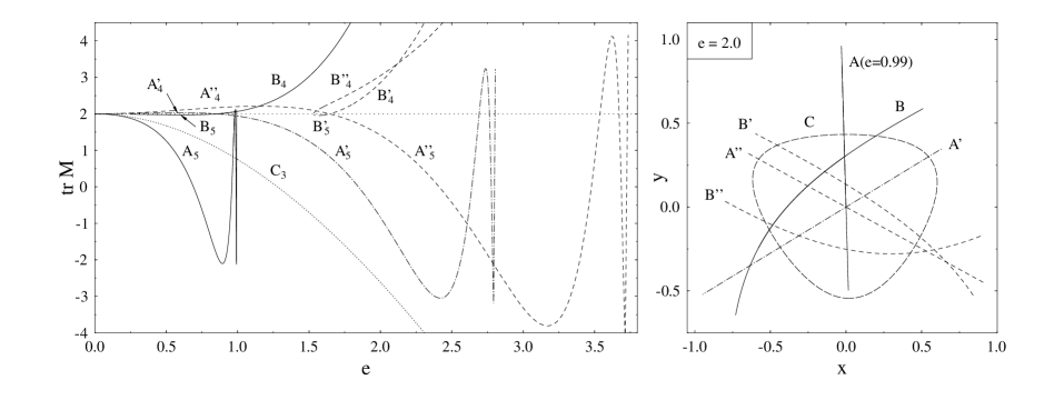
Figure 2: Left panel: Stability traces of A and B type orbits in the GHH potential with $\gamma=0.6$, $\beta=0.07$, plotted versus scaled energy $e$. The three saddles are at $e_{0}=0.993$, $e_{1}=2.81$, and $e_{2}=3.74$. Right panel: Shortest orbits, projected on the $(x,y)$ plane. Orbit A is evaluated at $e=0.99$ just below its saddle ($e_{0}=0.993$); all other orbits are taken at $e=2$. The line types correspond to those in the left panel.

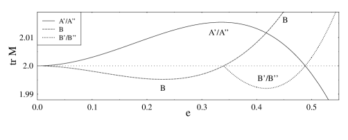
Figure 3: TCB of a degenerate pair of orbits A’, A” and B’, B” at $e_{tcb}=0.4889$ in the GHH potential with $\gamma=0.75$, $\beta=0$. The degeneracy is due to the reflection symmetry about the $y$ axis.

Another example of a TCB is shown in Fig. 3, obtained for the GHH potential with $\gamma=0.75$ and $\beta=0$. This potential is symmetric about the $y$ axis and therefore the pairs of orbits A’, A” and B’, B” are degenerate, lying opposite to each other with respect to the $y$ axis. The crossing happens at $e_{tcb}=0.4889$ and exhibits the same features as those discussed in the first example.

3.2.2 Characteristic properties of the TCB

We now discuss some of the properties of a TCB and compare our numerical results to their analytical predictions from the normal form of the TCB. For this purpose, we take the example at $e_{tcb}=0.854447$ seen in Fig. 2, where the orbits A’ and B bifurcate transcritically. Their crossing is shown in Fig. 4 on an enlarged scale in the upper left panel, where the numerical results for tr M$(e)$ are displayed by crosses (orbit A’) and circles (orbit B). We see that the graphs of tr M($e$) cross the critical line tr M = 2 with opposite slopes. Their Maslov indices, differing by one unit, are exchanged at the bifurcation (see Secs. 4 and 4.2). The upper right panel displays the numerical action difference $\Delta S=S_{B}-S_{A^{\prime}}$ (circles), where the action of each periodic orbit (po) is, as usual, given by

$$S_{po}=\oint{\bf p}\cdot{\rm d}{\bf q}\,.$$ (42)

In the lower panels, we show the shapes of the orbits in the $(x,y)$ plane below (left) and above (right) the TCB. The B orbit is seen to have passed through the A’ orbit at the bifurcation. The lengths of both orbits increase with energy $e$.

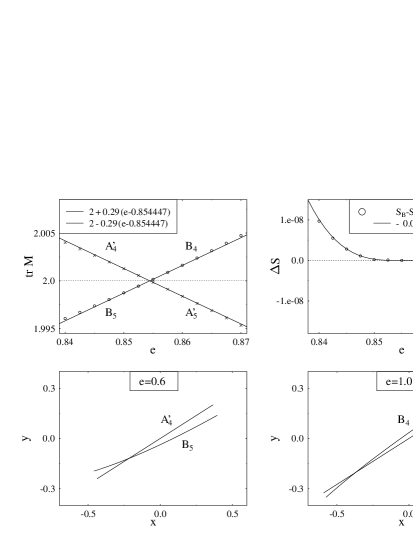
Figure 4: TCB in the GHH potential with $\gamma=0.6$, $\beta=0.07$. Orbits A’ and B exchange their stabilities (and Maslov indices $\sigma=$ 4,5) at $e_{tcb}=0.854447$. Upper left: tr M versus energy $e$; crosses (A’) and circles (B) are numerical results, solid lines the local prediction (98). Upper right: action difference $\Delta S$ versus $e$; circles are numerical results and the solid line the local prediction (99). Lower panels: shapes of the crossing orbits in the $(x,y)$ plane before and after the bifurcation.

The normal form of the TCB is derived and discussed in Sec. 6.2.3. From it, one can derive the local behavior of the actions, periods, and stability traces of the two orbits in the neighborhood of a TCB. For small deviations $\epsilon=c\,(e-e_{tcb})$ (with $c>0$) from the bifurcation energy, the stability traces go like tr M$(\epsilon)=2\pm 2\sigma\epsilon$, and the action difference of the two orbits like $\Delta S(\epsilon)=-\epsilon^{3}\!/6b^{2}$ (see App. 6.2.3 for the meaning of the other parameters). These local predictions, given in Fig. 4 by the solid lines, can be seen to be well followed by the numerical results.

The crossing of the graphs tr M($e$) of the two orbits at the bifurcation energy $e_{tcb}$ with opposite slopes is a characteristic feature of the TCB (see Sec. 2.2.1). Since the fixed points of the two orbits coincide at the bifurcation point, their shapes must be identical there. In the present example, the orbit B is a curved libration; the sign of its curvature is changed at the bifurcation, as illustrated in the two lower panels of Fig. 4.

We note that a completely different mechanism of stability exchange of two orbits, which happens through two close-lying PFBs, has been described in [40]. The stability diagram may then appear like that in the upper left of Fig. 4, if the crossing point is not analyzed with sufficient numerical resolution. Such a “false transcritical bifurcation” will be briefly discussed and illustrated in the appendix of our paper.

3.3 Stability and unfoldings of the TCB

Since the TCB is not a generic bifurcation according to Meyer’s list [11], we now address the question under which circumstances it can exist and what its structural stability is. The GHH systems discussed here have time-reversal symmetry, and it is therefore of interest to study the stability of the TCB under perturbations of the Hamiltonians that destroy this symmetry. In this context, it is important to note that a detailed mathematical study [18], in which all generic bifurcations in systems with time-reversal symmetry are classified, does not mention the TCB; the same holds also for [21]. So far we have only found TCBs which involve a straight-line libration. On the basis of the results presented in Sec. 2, we believe that in the class of all Hamiltonian systems containing a straight-line librating orbit, the TCB is actually the generic isochronous bifurcation of the librating orbit. Therefore, if we find a perturbation of the GHH system that destroys the time-reversal symmetry but preserves a straight-line libration, the TCB should also exist there. This will be demonstrated in Sec. 3.3.4 for a specific example.

A general Hamiltonian $H(x,y,p_{x},p_{y})$ supports the existence of a straight-line libration – which, without loss of generality, may be chosen to lie on the $y$ axis – if the following conditions are fulfilled:

$$\frac{\partial H}{\partial x}\,(0,y,0,p_{y})=0\,,\qquad\frac{\partial H}{\partial p_{x}}\,(0,y,0,p_{y})=0\,.$$ (43)

In the following we will first show how some TCBs are destroyed under perturbations that violate the conditions (43), and how they unfold. We find two types of unfoldings which are also discussed in [9, 22] for TCBs in non-Hamiltonian systems. In the first scenario, the TCB breaks up into SNBs. In the second scenario, no bifurcation is left in the presence of the perturbation and the functions tr M$(\epsilon)$ approach the critical line tr M = 2 without reaching it, so that one may speak of an avoided bifurcation. These scenarios can be described by the extended normal forms given in Sec. 6.2.4. We then also investigate perturbations that fulfill the criteria (43), allowing for the existence of TCBs in systems with or without any discrete symmetries.

3.3.1 Addition of a homogeneous transverse magnetic field

We first discuss the addition of a homogeneous magnetic field B = e_z$B_{0}$ to the Hamiltonian (38) which is transverse to the $(x,y)$ plane of motion. This is a situation that is frequently set up in experimental physics and gives us one important way of breaking of the time-reversal symmetry. The momenta $p_{i}$ ($i=x,y$) in (38) are replaced by the standard “minimal coupling”,

$$p_{i}\;\rightarrow\;p_{i}-\frac{e}{c}\,A_{i}\,,\qquad{\bf A}=\frac{1}{2}\,({\bf r}\times{\bf B})\,,$$ (44)

where ${\bf A}$ is the vector potential and $e$ the charge of the particle. This adds the following perturbation to the Hamiltonian:

$$\delta H(x,y,p_{x},p_{y})=\frac{eB_{0}}{2c}\,(xp_{y}-yp_{x})+\frac{1}{2}\left(\frac{eB_{0}}{2c}\right)^{\!2}(x^{2}+y^{2})\,,$$ (45)

which breaks the time-reversal symmetry of (38) due to the linear terms in $p_{x}$ and $p_{y}$, but also breaks the straight-line libration condition (43).

As an example, we choose the GHH potential with $\gamma=0.5$, $\beta=0.1$. Here the saddle energy for the A’ orbit is $e_{1}=3.83$; the other saddles are at $e_{0}=0.9852$ and $e_{2}=6.35$. In Fig. 5 we show the stability traces tr M$(e)$ of the orbits A’ and B’ with and without magnetic field. For $B_{0}=0$ (triangles and dashed-dotted lines), these orbits A’ and B cross at e${}_{bif}=1.42665$ in a TCB like in the examples discussed above. For $B_{0}\neq 0$ (circles and solid lines), they rearrange themselves into pairs A’${}_{\!4}$/B₅ and B₄/A’${\!{}_{5}}$ colliding in SNBs according to the prediction (104) of the normal form (103), in which $\kappa$ is taken proportional to the value of $B_{0}$.

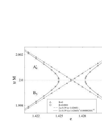
Figure 5: Unfolding of a TCB by a transverse magnetic field in the GHH potential with $\gamma=0.5$, $\beta=0.1$. Shown is tr M versus scaled energy $e$. Dashed lines and triangles: prediction (98) and numerical results for field strength $B_{0}=0$ of the unperturbed TCB; solid lines and circles: local prediction (104) (with an adjusted value of $\kappa$) and numerical results for $B_{0}=0.0001$.

3.3.2 Destruction of the TCB by a perturbation of the potential

Another example of the same unfolding of a destroyed TCB is shown in Fig. 6. Here the unperturbed GHH potential is the same as that used in Fig. 3 above, which is symmetric about the $y$ axis. This time we apply a perturbation of the potential alone

$$\delta V(x,y)=\kappa\,x^{\prime}y^{\prime 3}\,,$$ (46)

whereby $x^{\prime},y^{\prime}$ are rotated Cartesian coordinates such that the bifurcating A’ orbit lies on the $y^{\prime}$ axis. Clearly, this perturbation does not fulfill the conditions (43) (expressed in the rotated coordinates) and in fact destroys the original TCB of the orbits A and B’ shown in Fig. 3; the same fate happens also to the pair A” and B” of orbits. We see in Fig. 6 that, again, the original pairs of orbits on either side of the unperturbed TCB rearrange themselves such as to destroy each other in two pairs of SNBs, each according to the prediction (104) of the corresponding normal form. Since the effective perturbation strengths are different in the two original directions of the A’ and A” orbits, the splitting between the two pairs of SNBs is slightly different. A problem arises with the nomenclature of the perturbed orbits, which is somewhat ad hoc, since all perturbed orbits have become rotations. In the square brackets in the figure we indicate the names of the unperturbed orbits, of which A’, A” are straight-line and B’, B” curved librations (their stability traces are shown in Fig. 3 above). The stability traces of the perturbed orbits change drastically at the original bifurcations, but approach those of the unperturbed orbits sufficiently far from the bifurcations. The insert in the upper left of Fig. 6 illustrates one possible unfolding of a destroyed isochronous PFB (that seen at $e=0.34$ between the orbits B and B’/B” in Fig. 3) and will be commented in Sec. 3.3.5 below.

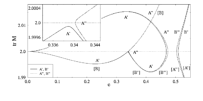
Figure 6: Unfolding of the TCB shown in Fig. 3 under the perturbation (46) with $\kappa=0.0001$ (see text for details). The labels in brackets [ ] correspond to the orbits of the unperturbed system in Fig. 3. For the insert, see Sec. 3.3.5.

3.3.3 An avoided TCB

In Fig. 7 we give an example of an avoided bifurcation. We start again from the same example as in Fig. 3, but now we apply the following perturbation:

$$\delta H(x,y,p_{x},p_{y})=\kappa^{\prime}\,x^{\prime 2}p_{y^{\prime}}\,,$$ (47)

again in the same rotated coordinates as for the perturbation (46) above. By construction, this perturbation does fulfill the libration-conservation conditions (43), expressed in the rotated coordinates ($x^{\prime},y^{\prime}$) for the orbit A’, so that the TCB of the orbits A’ and B’ survives. It will be discussed in more detail in the next subsection. The perturbation (47) destroys, however, the TCB of the original orbit pair A” and B” at $e_{tcb}=0.489$ and is seen to lead to an avoided bifurcation of the perturbed orbits, which are now called A” and B and shown by the heavy dashed lines. Their stability traces follow the local behavior (106) predicted by the normal form (105). Again, our nomenclature for the new orbits is not strict; the perturbed B” orbit has, for $e>0.489$, become a portion of the new orbit B. As in Fig. 6, the graphs tr M$(e)$ of the perturbed new orbits approach the unperturbed ones far from the bifurcations.

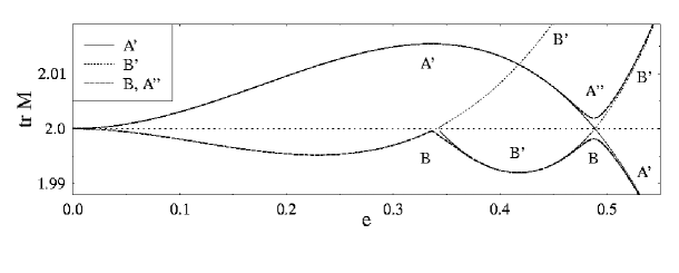
Figure 7: Unfolding of the TCB of the orbit pair A” and B” shown in Fig. 3 under the perturbation (47) with $\kappa^{\prime}=0.01$ into an avoided bifurcation of the new orbit pair A” and B near $e=0.489$ (shown by the heavy dashed lines). The surviving TCB of the orbit pair A’ and B’ (solid and thin dashed line, respectively) is commented in Sec. 3.3.4.

3.3.4 TCB in a system without any discrete symmetry

We now come to our last, and perhaps most interesting, example: a TCB in a system without any discrete symmetry. It is shown in Fig. 7 by the solid line for the orbit A’ and the thin dashed line for the orbit B’. It is the same as the TCB shown in Fig. 3 after applying the perturbation (47) that has been explicitly constructed so as to preserve the straight-line libration condition (43) in the rotated coordinates $x^{\prime}$, $y^{\prime}$. Here $y^{\prime}$ is the direction of the A’ orbit. Thus, the libration A’ in the perturbed system is identical to that in the unperturbed GHH potential ($\gamma=0.75$, $\beta=0$). The orbit B’, however, which in the unperturbed GHH system is a curved libration similar to that shown in Fig. 4, has now become a rotation except at the TCB point. While it was originally created, together with its symmetry-degenerate partner B”, in an isochronous PFB at $e=0.34$ from the original B orbit (see Fig. 3), this PFB is destroyed under the perturbation (47), and the perturbed B’ orbit is now created at a SNB at $e=0.343$. Its stable lower branch is that which crosses the unchanged A’ orbit transcritically at the slightly shifted new bifurcation energy $e_{tcb}=0.4886$.

The shapes of this perturbed B’ orbit in the rotated $(x^{\prime},y^{\prime})$ plane are shown in Fig. 8, on the left side in the energy region between its creation at $e=0.343017$ and its TCB at $e=0.4886$ where it is stable, and on the right side for the energies $e\geq 0.4886$ where it is unstable. Its librational shape at $e=0.4886$, where it is identical to the A’ orbit, is shown in both panels of the figure (note their different scales!).

Figure 8: Shapes of the B’ orbit, shown by the dashed line in Fig. 7, in the rotated $(x^{\prime},y^{\prime})$ plane at different energies. Left panel: stable region, at the energies $e=0.343$ (creation in SNB) – 0.4886 (TCB point). Right panel: unstable region, at the energies $e=0.4886$ (TCB point) – 4.0. Note the different scales in the two panels.

Figure 9: Same as Fig. 8 but in the rotated momentum space $(p_{x^{\prime}},p_{y^{\prime}})$.

In Fig. 9 we present the shapes of the B’ orbit in the rotated momentum space $(p_{x^{\prime}},p_{y^{\prime}})$. Here the orbit appears as a figure-8 type rotation, except at the TCB where it must be a straight-line libration, as the A’ orbit, also in momentum space. It should be noted that qualitatively, the shapes in momentum space are the same for all transcritically bifurcating B type orbits discussed in this paper, even if they remain curved librations in coordinate space.

One may interpret the perturbation (47) as the first-order expansion of a weak inhomogeneous magnetic field with strength proportional to $\kappa^{\prime}$. In a homogeneous field, for which the full perturbation is given in (45), the Lorentz force tends to turn all straight-line orbits into curved librations. In the system perturbed by (47), the Lorentz force of this inhomogeneous magnetic field is canceled, at least to lowest order, by the geometry of the total potential which tends to curve the librations the other way round. We leave it to the interested reader to speculate whether this scenario finds applications in accelerator physics, where one may want to produce straight-line trajectories in an inhomogeneous magnetic field.

3.3.5 Creation of a TCB in the unfolding of a PFB

In this section we will show how a TCB can be created by perturbing a PFB and how its existence may depend on particular symmetries. Two characteristic unfoldings of isochronous PFBs in one-dimensional dynamical systems have been described in [9, 10], which correspond to the “universal unfolding” of the isochronous PFB discussed extensively in [22]. We find the same unfoldings for the isochronous PFBs of the straight-line librations in the (G)HH potentials; one of them is of particular interest here as it leads to a TCB. The corresponding normal forms are given in App. 6.2.6.

In the first scenario, the original parent orbit does not change its stability, thus avoiding the bifurcation, and a pair of new orbits is created at a SNB. One of these new orbits takes the role of the original parent orbit after the bifurcation, and the perturbed parent orbit takes the role of one of the new orbits created at the original PFB. Examples of this scenario can be seen in Fig. 6 (inserted close-up) and in Fig. 7, as results of two different perturbations of the same original PFB seen in Fig. 3 at $e\sim 0.34$.

The second scenario is the unfolding into a SNB of a pair of new orbits, followed by a TCB of one of these orbits with the original parent orbit. An example of this has already been pointed out in Fig. 2 (left panel) to occur near $e\sim 1.62$, where the orbits B’ and B” bifurcate from the A” orbit. In the following we shall further illustrate this unfolding by explicitly perturbing a PFB in the standard HH system.

We start from the HH system, i.e., (38) with $\gamma=1$, $\beta=0$, and add the following perturbation to the potential

$$\delta V(x,y)=\frac{1}{3}\,\delta\,x^{3},$$ (48)

which destroys both the $C_{3v}$ symmetry and the reflection symmetry at the $y$ axis. It therefore affects the cascade of isochronous PFBs of the linear A orbit along the $y$ axis (cf. Sec 3.1.1). The perturbation (48) is chosen such as to preserve the straight-line libration condition (43), so that the A orbit still exists in its presence. To ensure the presence of a TCB in the perturbed system, we must fulfill the condition $P_{qq}\neq 0$ given in (19). An explicit expression for the quantity $P_{qq}$ in terms of the (total, perturbed) potential $V$ is given in (37). [In the integrand of (37), the function $V_{xxx}(x,y)$ is taken along the A orbit with $x(t)=0$, $y=y_{A}(t)$; see Sec. 2.3 for details and notation.] Since $V_{xxx}$ becomes nonzero with the perturbation (48), the occurrence of a TCB is possible. But $V_{xxx}\neq 0$ is not sufficient to ensure $P_{qq}\neq 0$: this will also depend on the symmetry of the function $\xi_{1}(t)$ appearing in the integrand of the quantity $P_{qq}$ in (37).

Now, as discussed in [27, 29], the functions $\xi_{1}(t)$ describe the $x$ motion (transverse to the A orbit) of the new orbits created at the successive PFBs of the A orbit. These functions are periodic Lamé functions with well-known symmetry properties. As it turns out, $\xi_{1}(t)$ of the L type orbits born at every second PFB of the cascade are even functions of $t$, where $t=0$ is the time at which $y_{A}(t)$ is maximum; whereas those of the R type orbits born at every other bifurcation are odd. The result is that $P_{qq}$ becomes zero at the R type bifurcations, in spite of $V_{xxx}\neq 0$, while $P_{qq}\neq 0$ for the L type bifurcations. Consequently, it is only at the L type bifurcation energies that a TCB can exist in the perturbed system. Our numerical investigations have confirmed that under the perturbation (48) all R type bifurcations remain, indeed, unbroken PFBs with unchanged stability traces tr M$(e)$ to first order in $\delta$, while the L type bifurcations are broken up as discussed above.

In Fig. 10 we show the creation of the orbits L₆ and L’₆ from the A orbit in the HH system under the perturbation (48). In the unperturbed HH system, these orbits are born as a degenerate pair from a PFB at the energy $e_{6}=0.986709235$ (cf. [27]), as also seen in Fig. 1. Here the PFB has been broken according to the second scenario described above, unfolding into a TCB of A_6/7 and L_7/6 at precisely the same critical energy $e_{tcb}=e_{6}$, and a SNB at $e_{6}-\Delta e_{6}\sim 0.98703$ where L₇ and L’₆ are born. The thin dash-dotted line gives the slope of tr M$(e)$ of the L orbit at the TCB which is minus that of the A orbit, as is characteristic of a TCB. The thin dotted line gives the slope of the original degenerate pair L₆, L’₆ created in the unperturbed HH system; this slope is minus twice that of the parent A orbit, as is typical of a PFB [see (23) in Sec. 2.2.2]. The same scenario is found at all successive L type bifurcations. In the perturbed system, the orbit pairs L, L’ are no longer degenerate, since the reflection symmetry at the $y$ axis is broken by (48). The graphs tr M$(e)$ seen in this figure are predicted by the normal form (113), as discussed explicitly in App. 6.2.6.

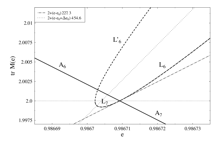
Figure 10: Creation of orbits L₆, L’₆ in a broken PFB in the HH potential under the perturbation (48) with $\delta=0.5$. The TCB of the orbits A and L occurs at the energy $e_{6}=0.986709235$ of the PFB of the degenerate pair L, L’ in the unperturbed HH potential [27]. (See text for the thin lines.)

4 Inclusion of a TCB in the semiclassical trace formula

4.1 The semiclassical trace formula

Our investigations have been largely motivated by the use of periodic orbits in the semiclassical description of the density of states $g(E)$ in a quantum system with discrete spectrum $\{E_{i}\}$

$$g(E)=\sum_{i}\delta(E-E_{i})\,.$$ (49)

Initiated by Gutzwiller (see [14] and earlier references therein), the periodic orbit theory (POT) [41] (see also [16, 25, 42] for general introductions) states that the oscillating part of the quantum density of states is given, to leading order in $\hbar$, by a semiclassical trace formula of the form

$$\delta g(E)=\sum_{po}{\cal A}_{po}(E)\,\cos\left(\frac{S_{po}(E)}{\hbar}-\frac{\pi}{2}\,\sigma_{po}\right).$$ (50)

The sum goes over all periodic orbits ($po$) of the classical system (including their repetitions), $S_{po}(E)$ are their actions (42) and $\sigma_{po}$ their Maslov indices (see [14, 43, 44, 45] and [25], appendix D, for details). The ${\cal A}_{po}(E)$ are semiclassical amplitudes which depend on the nature of the orbits. For orbits that are isolated in phase space, the amplitudes were given by Gutzwiller [14] as

$${\cal A}_{po}(E)=\frac{1}{\pi\hbar}\,\frac{T_{ppo}(E)}{\sqrt{|{\rm det\,[M}_{po}(E)-{\rm I}]|}}\,,$$ (51)

in terms of their primitive periods $T_{ppo}(E)=$ d$S_{ppo}(E)$/d$E$ and stability matrices M${}_{po}(E)$; here I is the unit matrix with the same dimension as M_po. For systems with continuous symmetries, in which most periodic orbits come in degenerate families (in particular in integrable systems), explicit expressions for the ${\cal A}_{po}(E)$ have been derived by various authors [46].

One problem with the Gutzwiller trace formula in mixed systems, where stable and unstable periodic orbits coexist, is the divergence of the amplitudes (51) occurring at bifurcations. Remedy is given by uniform approximations, introduced by Ozorio de Almeida and Hannay [47] (see also [17]) and further developed by several authors both for codimension-one [26, 48, 49] and codimension-two bifurcation scenarios [38, 50]. In the following sections, we will discuss the uniform approximations and derive its appropriate form for a pair of transcritically bifurcating orbits.

The trace formula (50) does not converge in mixed systems and most chaotic systems, in which the number of periodic orbits proliferates exponentially with increasing length, so that the summation over all orbits typically cannot be performed (see [15, 41]). In our study, we coarse-grain the density of states by convolution with a normalized Gaussian with width $\Delta E$, so that only the shortest orbits with periods $T_{po}\,\hbox{\kern 0.90005pt\lower 2.32501pt\hbox{$\sim$} \kern-10.07997pt\raise 2.32501pt\hbox{$<$} }\hbar/\Delta E$ contribute to the sum [25, 51, 52]. Although the finer details of the spectral information hereby are averaged out, the coarse-grained density of states

$$g_{\Delta E}(E)=\frac{1}{\sqrt{\pi}\Delta E}\sum_{i}e^{-(E-E_{i})^{2}\!/\Delta E^{2}}$$ (52)

still exhibits its gross-shell structure, provided that $\Delta E$ is not chosen too large. The correspondingly coarse-grained trace formula reads [25]

$$\delta g_{\Delta E}(E)=\sum_{po}{\cal A}_{po}(E)\,e^{-[T_{po}\,\Delta E/2\hbar]^{2}}\cos\left(\frac{S_{po}(E)}{\hbar}-\frac{\pi}{2}\,\sigma_{po}\right)\!,$$ (53)

where it can be seen that the additional exponential factor suppresses the contribution of longer orbits. This version of the POT has found many applications to gross-shell effects in finite fermion systems (see [25, 53] for examples).

4.2 Uniform approximation for bifurcating orbits

In this section we sketch the derivation for the combined contribution of a pair of bifurcating orbits A and B to the semiclassical trace formula (50) for the density of states. Since the individual amplitudes in the form (51) given by Gutzwiller diverge at the bifurcation, one has to go one step back in their evaluation and transform the trace integral to the phase space [26, 54, 55]. After doing the integration along the primitive A orbit with action $S_{A}(E)$, the remaining part of the trace integral is over the Poincaré surface of section in the variables $Q$ and $p$ transverse to the A orbit:

$$\delta g(E)\;=\;\Re e\;e^{\frac{i}{\hbar}S_{A}(E)-i\frac{\pi}{2}\sigma_{A}}\!\int\!{\rm d}Q\int\!{\rm d}p\;C(Q,p,\epsilon)\,e^{\frac{i}{\hbar}{\widetilde{S}}(Q,p,\epsilon)}.$$ (54)

The action function in the phase of the integrand is given by

$${\widetilde{S}}(Q,p,\epsilon)={\widehat{S}}(Q,p,\epsilon)-S_{A}(\epsilon)-Qp\,,$$ (55)

where ${\widehat{S}}(Q,p,\epsilon)$ is the generating function of the canonical transformation (4) that describes the Poincaré map, and $S_{A}(\epsilon)$ is the action integral (42) of the A orbit as a function of the control parameter $\epsilon$. By virtue of the canonical relations of the generating function

$$P=\frac{\partial{\widehat{S}}}{\partial Q}\,,\qquad q=\frac{\partial{\widehat{S}}}{\partial p}\,,$$ (56)

the stationary condition of the function ${\widetilde{S}}$ in the $(Q,p)$ plane for any fixed $\epsilon$,

$$\frac{\partial{\widetilde{S}}}{\partial Q}(Q_{0},p_{0},\epsilon)=\frac{\partial{\widetilde{S}}}{\partial p}(Q_{0},p_{0},\epsilon)=0\,,$$ (57)

yields $P_{0}=p_{0}$ and $Q_{0}=q_{0}$, so that the stationary points $(Q_{0},P_{0},\epsilon)=(q_{0},p_{0},\epsilon)$ of the phase function (55) are the fixed-point branches of the map and hence correspond to the periodic orbits. [Note that, by construction, ${\widetilde{S}}(q_{0},p_{0},\epsilon)=0$ along the fixed-point branch of the A orbit.]

The amplitude function $C(Q,p,\epsilon)$ in (54) is given [26] in terms of the generating function ${\widehat{S}}(Q,p,\epsilon)$ by

$$C(Q,p,\epsilon)=\frac{1}{2\pi^{2}\hbar^{2}}\,\frac{\partial{\widehat{S}}}{\partial E}(Q,p,\epsilon)\,.$$ (58)

Note that

$$\frac{\partial{\widehat{S}}}{\partial E}(Q,p,\epsilon)=:{\widehat{T}}(Q,p,\epsilon)=T_{A}(E)+\frac{\partial{\widetilde{S}}}{\partial E}(Q,p,\epsilon)\,,$$ (59)

where $T_{A}(E)=\frac{\rm d}{{\rm d}E}S_{A}(E)$ is the period of the A orbit.

In principle, the integration over $Q$ and $p$ in (54) is limited to that domain of the $(Q,p)$ plane which is accessible under energy conservation. However, in the spirit of the stationary-phase approximation (including its extensions below) we expect that, due to the rapidly oscillating phase of (54) in the semiclassical limit ${\widetilde{S}}\gg\hbar$, the main contributions to the integral come from small regions around the stationary points of the function ${\widetilde{S}}(Q,p,\epsilon)$. Assuming that the fixed points of A and the other orbit(s) taking part in the bifurcation are situated in the interior of this domain, and that no other bifurcations happen nearby, we may extend the integrals over both $Q$ and $p$ from $-\infty$ to $+\infty$.

Sufficiently far away from the bifurcation point $\epsilon=0$, so that the orbits A and B are isolated, the stationary-phase integration of (54) will yield precisely the contributions of the isolated orbits A and B to the standard Gutzwiller trace formula (50) with their individual amplitudes (51). Near the bifurcation, the stationary-phase approximation fails and one has to include higher than second-order terms in $Q$ and $p$ in the function ${\widetilde{S}}(Q,p,\epsilon)$. The simplest solution [17] is to use a truncated Taylor expansion of ${\widetilde{S}}(Q,p,\epsilon)$ in all three variables, keeping only the minimum number of terms necessary to be able to reproduce locally the fixed-point branches of all the orbits taking part in a given bifurcation. These truncated forms of ${\widetilde{S}}(Q,p,\epsilon)$ are the normal forms which are discussed in App. 6.

4.3 Uniform approximation for the TCB

Equipped with the normal form of the TCB given in App. 6.2.3, we now calculate the contribution of a pair of periodic orbits A and B undergoing a TCB to the semiclassical trace formula. We follow closely the treatment of [26], where uniform approximations for the generic bifurcations corresponding to [11, 17] were derived.

Since (54) is invariant under canonical transformation $(Q,p)\rightarrow(Q^{\prime},p^{\prime})$, we may think of the variables $Q,p$ to be the adapted coordinates for which (85) and the equations given thereafter are valid. We are therefore allowed to insert for ${\widetilde{S}}(Q,p,\epsilon)$ the normal form derived in Sec. 6.2.3 for the TCB, in order to derive the uniform approximation to the trace formula which includes the orbits taking part in the TCB.

We will do this in two steps. First, we evaluate (54) only at $\epsilon=0$. This yields the so-called local uniform approximation in the spirit of Ozorio de Almeida and Hannay [47]. In the second step, we use the full normal form (96) and the corresponding functions $C(Q,p,\epsilon)$ defined by (58) to find, after some suitable transformations, the global uniform approximation in the spirit of [26, 48, 49]. The latter yields asymptotically the Gutzwiller trace formula for the orbits A and B sufficiently far from the bifurcation.

We now use for ${\widetilde{S}}(Q,\epsilon)$ the normal form (101) of the TCB (omitting the tilde on the variables $Q,p,\epsilon$ and on $b$). Using the relation (3), the function ${\widehat{T}}$ in (59) becomes

$${\widehat{T}}(Q,\epsilon)=T_{A}(E)-Q^{2}\,.$$ (60)

After the elementary $p$ integration, yielding a complete Fresnel integral, we obtain for (54)

$$\delta g(E)\;=\;\frac{1}{\pi\hbar\sqrt{2\pi\hbar}}\,\Re e\;e^{\frac{i}{\hbar}S_{A}(E)-i\frac{\pi}{2}(\sigma_{A}+\frac{1}{2})}\left[T_{A}(E)\,F(b,\epsilon)-G(b,\epsilon)\right],$$ (61)

where we have defined the two following one-dimensional integrals

$$F(b,\epsilon) := \int_{-\infty}^{\infty}\!{\rm d}Q\,e^{-\frac{i}{\hbar}\,(\epsilon Q^{2}+bQ^{3})},$$ (62)

$$G(b,\epsilon) := \int_{-\infty}^{\infty}\!{\rm d}Q\,Q^{2}\,e^{-\frac{i}{\hbar}\,(\epsilon Q^{2}+bQ^{3})}=i\hbar\,\frac{\partial}{\partial\epsilon}F(b,\epsilon)\,.$$ (63)

Using the substitution $Q=x-{\tilde{Q}}$ with ${\tilde{Q}}=\epsilon/3b$, we obtain

$$F(b,\epsilon)=2\pi\left(\frac{\hbar}{3|b|}\right)^{\!1/3}e^{\frac{i}{\hbar}\Delta S(\epsilon)}\,{\rm Ai}(-z^{\prime})\,,\qquad z^{\prime}=\frac{\epsilon^{2}}{(3|b|)^{4/3}\hbar^{2/3}}\,,$$ (64)

where Ai is the Airy function (see [58], 10.4) and

$$\Delta S(\epsilon)=-\frac{2\epsilon^{3}}{27\,b^{2}}\,.$$ (65)

Using the r.h.s. of (63) to calculate $G(b,\epsilon)$, we finally obtain for the level density

$$\delta g(E) \!=\! \frac{\sqrt{2}}{\sqrt{\pi}\,\hbar^{7/6}\,(3|b|)^{1/3}}\,\Re e\;e^{i\left[\frac{1}{\hbar}S_{A}(E)+\Delta S(\epsilon)-\frac{\pi}{2}(\sigma_{A}+\frac{1}{2})\right]}$$ (66)

$$\hskip 91.04872pt\times\left[\left(T_{A}(E)+\frac{2\epsilon^{2}}{9b^{2}}\right){\rm Ai}(-z^{\prime})+i\,\frac{2\epsilon}{(3|b|)^{4/3}}\,\hbar^{1/3}{\rm Ai}^{\prime}(-z^{\prime})\right]\!.$$

4.3.1 Local uniform approximation

We first give the result (66) for $\epsilon=0$, using the known value [58] of Ai(0), to find the local uniform level density at the bifurcation energy $E_{0}$:

$$\delta g_{loc}(E_{0})=\frac{T_{A}(E_{0})\,\Gamma(\frac{1}{3})}{\pi\sqrt{6\pi}\,\hbar^{7/6}\,|b|^{1/3}}\,\cos\left[\frac{1}{\hbar}S_{A}(E_{0})-\frac{\pi}{2}\,\sigma_{A}-\frac{\pi}{4}\right]\!,$$ (67)

which contains the combined contribution of both orbits A and B taking part in the transcritical bifurcation. An explicit expression for the calculation of the normal form parameter $b$ is given in (37) of Sec. 2.3. The result (67) looks identical to that obtained in [26] for the generic SNB. The reason is that the normal form for this bifurcation is [26] $\widetilde{S}(Q,p,\epsilon)=-\epsilon\,Q-b\,Q^{3}-\sigma\,p^{2}/\!2$ which for $\epsilon=0$ gives, of course, the same result as the normal form (101). Note that the power 7/6 of $\hbar$ in the denominator is by 1/6 higher than in the semiclassical amplitude (51) of an isolated orbit.

4.3.2 Global uniform approximation

The result (67) gives the correct semiclassical amplitude of the bifurcating pair of orbits A and B only locally at the bifurcation, i.e., for $\epsilon=0$. We want, however, to know it also away from the bifurcation, and in particular, also in the limit where it can be written as a sum of the two individual contributions of the isolated orbits A and B to the standard Gutzwiller trace formula (50). To achieve this, we note that if we use the asymptotic forms of the Airy function and its derivative in (66) for $|z^{\prime}|\gg 1$, we obtain two terms that formally look like contributions to (50) with amplitudes of the form (51), but with the actions $S_{po}(E)$, periods $T_{po}(E)$, and stability traces tr M${}_{po}(E)$ replaced by their expansion to lowest order in $\epsilon$, as found from the normal form and given in (98) and (99).

The next intuitively obvious step is therefore to rewrite the asymptotic form of (66) in terms of the locally expanded quantities $S_{po}(\epsilon)$, $T_{po}(\epsilon)$, and tr M${}_{po}(\epsilon)$ of the two orbits ($po$ = A,B) and then to replace them by the correct functions $S_{po}(E)$, $T_{po}(E)$, and tr M${}_{po}(E)$ found numerically for the isolated orbits away from the bifurcation. This step has been rigorously justified in [26] by some appropriate transformations and need not be repeated here. The calculation goes exactly like that presented in [26] for the case of the SNB on that side where both orbits are real. The reason is that although the normal forms of the two bifurcations are different, they lead to identical integrals after a translation in the integration variable $Q$.

The result is the following uniform contribution of the two bifurcating orbits to the Gutzwiller trace formula:

$$\delta g_{un}(E)=\sqrt{6\pi\xi}\left\{\frac{\overline{\cal A}(E)}{\sqrt{z}}\,\cos\left(\frac{\overline{S}(E)}{\hbar}-\frac{\pi}{2}\,{\overline{\sigma}}\right)\!{\rm Ai}(-z)-\frac{\Delta{\cal A}(E)}{z}\,\sin\left(\frac{\overline{S}(E)}{\hbar}-\frac{\pi}{2}\,{\overline{\sigma}}\right){\rm Ai}^{\prime}(-z)\right\}.$$ (68)

The quantities occurring in (68) are defined as

$$z = (3\xi/2)^{2/3}\,,\qquad\qquad\quad\,\xi\;\;=\;\;\frac{1}{2\hbar}\,|S_{A}-S_{B}|\,,$$

$${\overline{S}} = \frac{1}{2}\,(S_{A}+S_{B})\,,\qquad\quad\;\;{\overline{\sigma}}\;\;=\;\;\frac{1}{2}\,(\sigma_{A}+\sigma_{B})\,,$$

$${\overline{\cal A}} = \frac{1}{2}\,({\cal A}_{A}+{\cal A}_{B})\,,\qquad\;\Delta{\cal A}\;\;=\;\;\frac{1}{2}\,({\cal A}_{A}-{\cal A}_{B})\,{\rm sign}(S_{A}-S_{B})\,,$$ (69)

all to be taken at the energy $E$, where $S_{po}(E)$ and $\sigma_{po}$ are the actions and Maslov indices, respectively, of the isolated periodic orbits on either side of the bifurcation, and ${\cal A}_{po}(E)>0$ are their Gutzwiller amplitudes (51).

At the bifurcation ($\epsilon=z=\xi=0$), the result (68) reduces to the local uniform approximation (67). Far enough away from the bifurcation, it goes over to the contribution of the isolated orbits A and B to the standard Gutzwiller trace formula. Indeed, expressing the Airy function in terms of Bessel functions as [58]

$${\rm Ai}(-z) = \frac{1}{3}\,\sqrt{z}\left[J_{1/3}(\xi)+J_{-1/3}(\xi)\right],$$

$${\rm Ai}^{\prime}(-z) = \frac{1}{3}\,z\left[J_{2/3}(\xi)-J_{-2/3}(\xi)\right],$$ (70)

and using their asymptotic form

$$J_{\nu}\longrightarrow\sqrt{\frac{2}{\pi\xi}}\,\cos\left(\xi-\frac{\pi}{2}\,\nu-\frac{\pi}{4}\right)\qquad\hbox{ for }\qquad\xi\gg 1\,,$$ (71)

we obtain from (68) for $\xi\gg 1$, i.e., for $|S_{A}-S_{B}|\gg 2\hbar$, the sum of the isolated Gutzwiller contributions to the trace formula

$$\delta g(E)=\sum_{po=A,B}{\cal A}_{po}(E)\,\cos\left(\frac{S_{po}(E)}{\hbar}-\frac{\pi}{2}\,\sigma_{po}\right),$$ (72)

with the amplitudes ${\cal A}_{po}(E)$ given in (51).

For the reason given above, the result (68) looks identical to that given in [26] for the SNB on that side where the two orbits are real. The present result holds on both sides of the TCB and can easily be seen to yield asymptotically the result (72) on both sides, with the roles of the orbits A and B and their Maslov indices properly exchanged.

4.4 Numerical test

We present here a numerical calculation of the density of states, both quantum-mechanical and semiclassical, of the GHH Hamiltonian (38) with $\gamma=0.6$, $\beta=0.07$, whose shortest orbits and stability traces are shown in Fig. 2. The parameter $\alpha$ in the Hamiltonian (38) has been chosen as $\alpha=0.04$. The three saddles then lie at the energies $E_{0}\simeq 103$, $E_{1}\simeq 293$ and $E_{2}\simeq 390$ in units such that the spacing of the harmonic-oscillator spectrum reached in the limit $E\to 0$ equals $\hbar\omega=1$. (See Fig. 2 for the scaled energies $e_{0},$ $e_{1}$ and $e_{2}$ of the saddles.)

The spectrum of the quantum-mechanical Hamiltonian corresponding to (38) has been obtained by diagonalization in a two-dimensional harmonic oscillator basis. Strictly speaking, the spectrum is not discrete since the system has no lower bound. However, for energies below the three saddles, the tunneling probabilities are exponentially small. In principle, the semiclassical trace formula can also be applied in the continuum region above the saddles, if the (complex) energies of the resonances are used to calculate the density of states. For a detailed discussion of this situation, we refer to [39] where a semiclassical calculation has been successfully performed for the standard HH system up to twice the saddle energy. In the present system, the discrete energies obtained for $E_{0}\,\hbox{\kern 0.90005pt\lower 2.32501pt\hbox{$\sim$} \kern-10.07997pt\raise 2.32501pt\hbox{$<$} }E\,\hbox{\kern 0.90005pt\lower 2.32501pt\hbox{$\sim$} \kern-10.07997pt\raise 2.32501pt\hbox{$<$} }150$ in the numerical diagonalization turn out to be good approximations to the real parts of the resonance energies, while the imaginary parts of the resonances are still negligible.

For our present test, we have chosen a coarse-graining width in (52) of $\Delta E=0.6$. This allows us to restrict the summation over the periodic orbits ($po$) to the primitive (“period one”) orbits; including second or higher repetitions does not affect the numerical results within the resolution of the lines presented in the figure below. As we can see in Fig. 2 (left panel), there exist only five “period one” orbits in the system below the scaled energy $e\simeq 1.5$ corresponding to $E\simeq 156$.

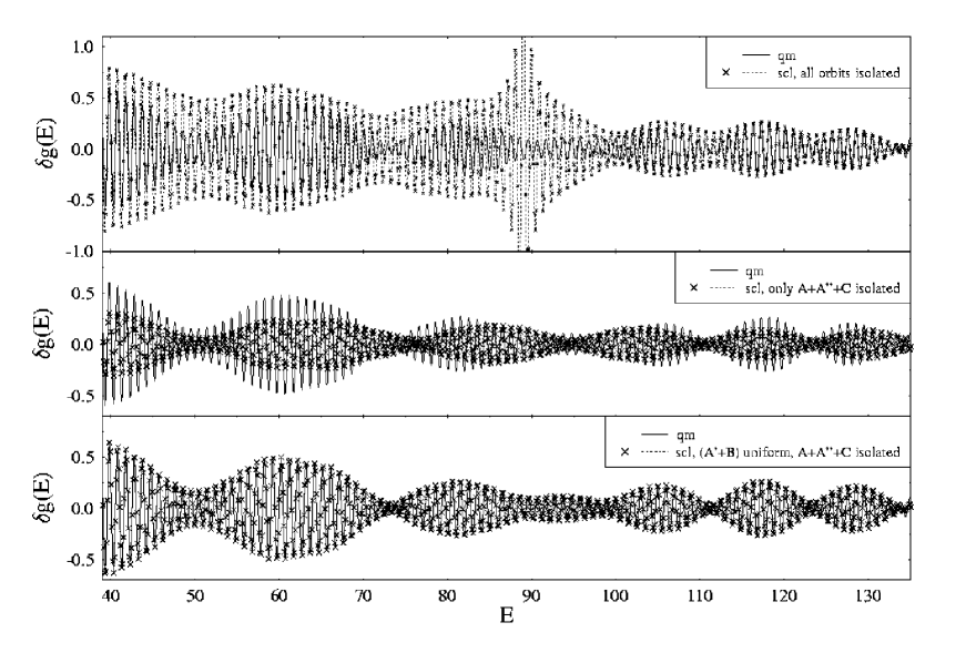
Figure 11: Oscillating part $\delta g(E)$ of the density of states in the GHH potential (38) with $\gamma=0.6$, $\beta=0.07$ and $\alpha=0.04$, plotted versus the unscaled energy $E$. The quantum-mechanical (qm) results are shown by the solid lines (identical in all three panels), different semiclassical (scl) approximations are shown by the crosses. Both qm and scl results have been coarse-grained by a Gaussian with width $\Delta E=0.6$, see (52). Top: the five shortest (primitive) orbits A, B, C, A’ and A” are included by the standard Gutzwiller trace formula (51), (53) for isolated orbits. Note the divergence near $E=89$, corresponding to $e_{tcb}=0.854447$ where the TCB of orbits A’ and B occurs (cf. Fig. 4). Middle: same as in the top panel, but the two crossing orbits A’ and B are omitted. Bottom: same as in the middle panel, but now the crossing orbits A’ and B are added in the global uniform approximation (68).

In Fig. 11, we show the oscillating part of the level density obtained for $\alpha=0.04$ as a function of the unscaled energy $E$, up to $E=135$ which corresponds to $e\simeq 1.3$. The solid lines display the coarse-grained quantum-mechanical result which is the same in all three panels. In order to extract the oscillating part of the quantum density of states (52), we subtracted its Strutinsky averaged part which here corresponds to the Thomas-Fermi approximation [25]. The crosses, connected by dashed lines, represent the semiclassical result in various approximations. The regular fast oscillations with period $\sim 1$ on the energy scale $E$ come from the common average action $S_{po}(E)$ of the leading periodic orbits, which becomes the action $S_{ho}(E)=2\pi E$ of the harmonic oscillator in the limit $E\to 0$. The beat-like slow variation in the amplitude of $\delta g(E)$ is due to the interferences of the periodic orbits and can be captured by the semiclassical trace formula (53).

In the top panel of Fig. 11, the five orbits A, B, C, A’ and A” are included in the trace formula (53) with their Gutzwiller amplitudes (51). Although they qualitatively reproduce the main trends of the beating density of states, they overestimate it. One can clearly see the divergence at $E\simeq 89$ corresponding to the scaled energy $e_{tcb}=0.854447$, where the TCB of the orbits A’ and B occurs. (The divergences due to the PFB sequence of the orbit A near $e=0.993\leftrightarrow E=103.5$ cannot be seen with this resolution.) The center panel shows the same semiclassical result, but omitting the contributions of the bifurcating orbits A’ and B. Clearly, the agreement with quantum mechanics is not good even far from the bifurcation, showing that these orbits always play a role. In the bottom panel, the orbits A, C and A” are again included as isolated orbits with the amplitudes (51), while the combined contribution of the bifurcating orbits B and A’ is included in the global uniform approximation given in (68). The agreement between semiclassics and quantum mechanics is now excellent, demonstrating the adequacy of the uniform approximation. The fact that the isolated-orbit approximation in the top panel does not work even far away from the bifurcation shows that the orbits A’ and B do not become isolated enough in the energy region shown; i.e., the asymptotic form (72) of the uniform approximation is not reached. This could already be expected from the fact that the stability traces tr M$(e)$ of these orbits stay very close to +2 for all $e<1.2$, as can be seen in Fig. 2.

In the energy limit $E\to 0$ (not shown in Fig. 11), the present semiclassical approximations are not appropriate due to the integrable limit of the harmonic oscillator. A corresponding uniform approximation for the standard HH potential has been derived in [37]. It can be generalized in a straightforward manner to the GHH systems, following the lines of [37], but this would lead beyond the scope of the present paper.

5 Summary

We have discussed transcritical bifurcations (TCBs) of periodic orbits in non-integrable two-dimensional autonomous Hamiltonian systems. We have first discussed the mathematical aspects of the TCB, making use of recent studies by Jänich [12, 13]. We then have, with the help of numerical examples in generalized Hénon-Heiles (HH) systems, discussed their phenomenology and their unfoldings under perturbations. We have shown, in particular, that a TCB may also exist in a system without any discrete symmetry, although it does not belong to Meyer’s list [11] of generic bifurcations. The reason is our restriction to systems containing straight-line librations. In such systems, the TCB appears to be the generic isochronous bifurcation of the straight-line libration while its isochronous pitchfork bifurcation (PFB) represents an exception expressed by the condition $P_{qq}=0$ in (19). Using this condition and the explicit expression (37) for the calculation of $P_{qq}$ for Hamiltonians of the form (25), we have exploited a special type of unfolding of the PFB to construct a perturbation of the standard HH system under which the TCB occurs.

So far, we have only encountered TCBs of straight-line librational orbits. In most examples, the second orbit that takes part in the TCB with the straight-line libration is also a librational orbit, though not along a straight line. That this need not be so has been shown in the example in Fig. 8, where the second orbit is a rotation (except, of course, at the TCB where it coincides with the straight-line libration). This system, in the presence of the momentum-dependent perturbation (47), is the only example of a Hamiltonian which does not have the form (25) and in which we found a transcritically bifurcating straight-line orbit. From the general criteria given in Sec. 2.2, however, we see no a priori reason why rotational orbits should not undergo TCBs as well. Furthermore, it is obvious that a given straight-line orbit can always transformed into a more complicated one by suitable canonical transformations. The inverse question – if an arbitrary nonlinear periodic orbit can be canonically transformed into a straight-line libration which can bifurcate transcritically – might also have a positive answer, but we see no way of proving or testing this, nor can we give a nontrivial example, since periodic orbits (except straight-line librations) in non-integrable systems usually cannot be given analytically.

Finally, we have constructed a global uniform approximation for the inclusion of transcritically bifurcating periodic orbits in the semiclassical trace formula for the quantum density of states. A numerical comparison with the fully quantum-mechanical calculation of the coarse-grained density of states yields excellent agreement. The normal forms of the TCB and the isochronous PFB have been derived in the appendix, where we also point to a “false TCB” which is the result of a stability exchange between different orbits via an intermediate periodic orbit through a pair of PFBs.

Acknowledgments

We are very grateful to K Jänich for his vivid interest in our work and for critical and helpful comments to this manuscript. We also acknowledge encouraging discussions with J Delos, B Eckhardt, S Fedotkin, A Magner, J Main, M Sieber and G Tanner.

6 Appendix 1: Normal forms

In singularity theory (see, e.g., [22]) and catastrophe theory (see, e.g., [56]) it is standard to classify bifurcations according to their normal forms. In App. 6.1 we briefly discuss normal forms for isochronous bifurcations in non-Hamiltonian one-dimensional systems and give the explicit forms for the TCB, the PFB and the saddle-node bifurcation (SNB).

While non-Hamiltonian fields can always be transformed to normal forms by suitable coordinate transformations, the situation is more complicated for Hamiltonian fields [57]. Here the normal forms depend on pairs of canonical variables, like the Poincaré variables $(q,p)$ used in Sec. 2, and must be derived, for a given Hamiltonian and a given type of bifurcating orbit, from the generating function ${\widehat{S}}(Q,p,\epsilon)$ of the Poincaré map or, equivalently, from the function ${\widetilde{S}}(Q,p,\epsilon)$ given in (55), by suitable canonical transformations. The strength of the normal forms – if they can be found – is that they are unique for each generic type of bifurcation and do not depend on the particular form of the Hamiltonian or the bifurcating orbit. However, the reduction of ${\widetilde{S}}(Q,p,\epsilon)$ to one of these generic normal forms is, according to Arnold [57], “generally not possible, and formal series for canonical transformations reducing a system to normal form generally diverge”.

Nevertheless, for the generic bifurcations occurring in two-dimensional symplectic maps, as analyzed and classified by Meyer [11], normal forms suitable for semiclassical applications have been given in [17, 47].

6.1 Normal forms for one-dimensional non-Hamiltonian systems

We follow here the book of Golubitsky and Schaeffer [22] and use their notation. In a simple one-dimensional problem with a “state variable” $x$ and a “bifurcation parameter” $\lambda$, one may study the set of values $(x,\lambda)$ satisfying the equation

$$g(x,\lambda)=0\,,$$ (73)

where $g(x,\lambda)$ is a differentiable scalar function of both arguments. Bifurcations of this set occur at critical points $(x_{0},\lambda_{0})$ where

$$\left.g_{x}(x_{0},\lambda_{0})=\frac{\partial}{\partial x}\,g(x,\lambda)\right|_{x_{0},\lambda_{0}}=0\,.$$ (74)

The TCB can be specified by the following criteria: at the critical point $(x_{0},\lambda_{0})$, the function $g$ must fulfill

$$g=g_{x}=g_{\lambda}=0\,,\qquad g_{xx}\neq 0\,,\qquad{\rm det}\,d^{2}g=g_{xx}\,g_{\lambda\lambda}-g_{x\lambda}^{2}<0\,,$$ (75)

where the subscripts denote partial derivatives with respect to the corresponding variables. For the fixed points $x_{n}=x_{n+1}=x$ of the quadratic map (1), we get the function $g(x,r)=rx(1-x)-x$ which fulfills the criteria (75) with $\lambda=r$ at the critical point ($x_{0}=0,r_{0}=1$), so that a transcritical bifurcation must occur there.

Normal forms are the simplest functions, usually taken to be polynomial forms in $x$ and $\lambda$, which obey the criteria for a given bifurcation. They can often be found by Taylor expansion of a given equivalence class of functions around the critical points, keeping the lowest necessary number of terms required to fulfill the given criteria. A valid normal form for the TCB is [23]

$$g_{tcb}(x,\lambda)=\pm x^{2}-\lambda\,x\,,$$ (76)

which fulfills the criteria (75) at $(x_{0},\lambda_{0})=(0,0)$. Normal forms are not unique. The following form is easily seen to be strongly equivalent (in the sense of [22]) to (76):

$$g_{sb}(x,\lambda)=\pm x^{2}-\lambda^{2},$$ (77)

since it also fulfills the criteria (75) at $(x_{0},\lambda_{0})=(0,0)$. Although the bifurcation corresponding to (77) in [22] is referred to as “simple bifurcation”, it is identical to what we here call the TCB.

The criteria for the isochronous PFB are [22, 23]

$$g=g_{x}=g_{\lambda}=g_{xx}=0\,,\qquad g_{x\lambda}\neq 0\,,\qquad g_{xxx}\neq 0\,,$$ (78)

and its standard normal form is

$$g_{pfb}(x,\lambda)=\pm x^{3}-\lambda\,x\,.$$ (79)

For completeness we give here also the criteria for the SNB (or tangent) bifurcation (in [22] called “limit point”):

$$g=g_{x}=0\,,\qquad g_{\lambda}\neq 0\,,\qquad g_{xx}\neq 0\,,$$ (80)

and its normal form:

$$g_{snb}(x,\lambda)=\pm x^{2}-\lambda\,.$$ (81)

Golubitzky and Schaeffer [22] also list the “isola center” bifurcation whose criteria are:

$$g=g_{x}=g_{\lambda}\,,\qquad g_{xx}\neq 0\,,\qquad{\rm det}\,d^{2}g>0\,,$$ (82)

with the normal form

$$g_{ic}(x,\lambda)=\pm(x^{2}+\lambda^{2})\,.$$ (83)

In two-dimensional Hamiltonian systems, the isola center is, according to Jänich’s classification [12], a rank 1 bifurcation for which the Hessian matrix K in (17) is regular and definite.

6.2 Normal forms for crossing bifurcations

In order to find normal forms for the two types of crossing bifurcations discussed in this paper, which we need in the semiclassical trace formula (54), we follow the heuristic approach of determining a truncated Taylor expansion of ${\widetilde{S}}(Q,p,\epsilon)$ with the minimum number of terms necessary to describe the required properties of these bifurcations. To this purpose, we first establish relations between the partial derivatives of the functions $Q(q,p,\epsilon)$ and $P(q,p,\epsilon)$ in (4), and the partial derivatives of the function ${\widetilde{S}}(Q,p,\epsilon)$ for which we use the same notation as in 2.1. Translating the criteria given in Sec. 2.2 for the crossing bifurcations in terms of the partial derivatives of ${\widetilde{S}}$, we can determine the normal forms of the TCB and the FLB. Although the formal transformations needed to arrive at these normal forms are not necessarily canonical, their use in the semiclassical trace formula can be justified by the fact that possible missing terms of higher order do not affect the results to leading order in $\hbar$ (cf. [17, 26, 48, 49]).

6.2.1 Relations between $Q,P$ and $\widetilde{S}$ and their partial derivatives

From (55) and (56) we obtain the following basic relations

$$Q(q,p,\epsilon) = q-{\widetilde{S}}_{p}(Q,p,\epsilon)\,,$$

$$P(q,p,\epsilon) = p+{\widetilde{S}}_{Q}(Q,p,\epsilon)\,.$$ (84)

We now take partial derivatives of these relations with respect to the variables $q$, $p$ and $\epsilon$, in order to formulate the conditions for the crossing bifurcations discussed in Sec. 2.2 in terms of partial derivatives of the function ${\widetilde{S}}(Q,p,\epsilon)$. This procedure is simplified by the following step. The splitting lemma of catastrophe theory (see [56], pp 95 and 103) states that after a suitable (but perhaps not canonical) coordinate transformation, the function ${\widetilde{S}}(Q,p,\epsilon)$ can be split up in the following way

$${\widetilde{S}}(Q,p,\epsilon)=S(Q,\epsilon)-\frac{\sigma}{2}\,p^{2},\qquad\sigma\neq 0\,,$$ (85)

where $S(Q,\epsilon)$ does not depend on $p$ any more. In the suitably adapted coordinates $q,p$ and $Q,P$ for which (85) is true, we obtain the following relations

$$\!\!\!\!\!\!\!\!\!\!\!\!\!\!\!Q_{q}(\epsilon)=1\,, \quad Q_{p}(\epsilon)=-{\widetilde{S}}_{pp}(\epsilon)=\sigma\,,$$ (86)

$$P_{q}(\epsilon)\,=S_{QQ}(\epsilon)\,, \quad P_{p}(\epsilon)\,=1+\sigma\,S_{QQ}(\epsilon)\,,$$

and ${\rm tr\,M}(\epsilon)$ becomes

$${\rm tr\,M}(\epsilon)=2+\sigma\,S_{QQ}(\epsilon)\,,$$ (87)

which is valid along the fixed-point branches of both orbits A and B. We also give some of the higher partial derivatives of $Q$ and $P$ at $\epsilon=0$ (valid in the adapted coordinates):

$$Q_{qq}=0\,,\quad Q_{qp}=0\,,\quad P_{qq}=S_{QQQ}\,,\quad P_{qp}=\sigma\,S_{QQQ}\,,$$ (88)

and

$$P_{q\epsilon}=S_{QQ\epsilon}\,,\quad P_{qqq}=S_{QQQQ}\,.$$ (89)

6.2.2 Criteria for the two crossing bifurcations

We can now express the criteria for the two types of crossing bifurcations introduced in Sec. 2.2 directly in terms of the parameter $\sigma$ and the partial derivatives of the function $S(Q,\epsilon)$ defined in (85). To have a bifurcation of the A orbit at $\epsilon=0$, we must have

$$S_{QQ}(Q=0,\epsilon=0)=0\,.\qquad(\hbox{\it bifurcation~{}of~{}A~{}orbit})$$ (90)

For the occurrence of a rank 1 bifurcation, we have the criterion (see the end of Sec. 2.1)

$$P_{\epsilon}=S_{Q\epsilon}=0\,.\qquad(\hbox{\it rank~{}1~{}bifurcation})$$ (91)

Since $(P,Q)=(p,q)=(0,0)$ then is the fixed-point branch of the A orbit for all $\epsilon$, the function $S(Q,\epsilon)$ must fulfill, due to (84), the condition

$$S_{Q}(0,\epsilon)=0\qquad\forall\,\epsilon\,.\qquad(\hbox{\it fixed-point~{}branch~{}of~{}A~{}orbit})$$ (92)

The criterion for the occurrence of a crossing bifurcation is that the slope ${\rm tr}\,{\rm M}_{\rm A}^{\prime}(0)$ given by (12) be nonzero, see also (18). We therefore need

$$S_{pp}=-\sigma\neq 0\,,\quad S_{QQ\epsilon}\neq 0\,.\qquad(\hbox{\it crossing~{}bifurcation})$$ (93)

The criterion for this bifurcation to be transcritical is

$$S_{QQQ}\neq 0\,.\qquad(\hbox{\it transcritical~{}bifurcation})$$ (94)

For the occurrence of a fork-like bifurcation, we must have

$$S_{QQQ}=0\,,\qquad S_{QQQQ}\neq 0\,.\qquad(\hbox{\it fork-like~{}bifurcation})$$ (95)

We are now ready to construct the simplest normal forms for the function ${\widetilde{S}}(Q,p,\epsilon)$, split like in (85), that fulfill all the above criteria (90) - (93) and either (94) or (95).

6.2.3 Normal form of the TCB

For the transcritical bifurcation, the normal form obtained in this way is

$${\widetilde{S}}(Q,p,\epsilon)=-\,\epsilon\,Q^{2}-b\,Q^{3}-\frac{\sigma}{2}\,p^{2}\,,\qquad(b\neq 0)$$ (96)

with $b=-\frac{1}{6}\,P_{qq}$. An explicit formula for calculating $P_{qq}$ and hence the parameter $b$ is given in (37). The normal form (96) corresponds to that of the TCB in non-Hamiltonian systems given in (76) in App. 6.1, if we choose ${\widetilde{S}}_{Q}(Q,p$=$0,\epsilon)=g_{tcb}(q,\epsilon)$, but it has, to our knowledge, not been discussed in connection with bifurcations of periodic orbits in Hamiltonian systems.

The fixed-point branch of the B orbit is easily found to be

$$p_{B}(\epsilon)=0\,;\qquad Q_{B}(\epsilon)=-\frac{2}{3b}\,\epsilon\quad\Leftrightarrow\quad\epsilon_{B}(Q)=-\frac{3b}{2}\,Q\,.$$ (97)

The stability traces of the two orbits are then found from (87) to be

$${\rm tr}\,{\rm M}_{\rm A}(\epsilon) = 2-2\sigma\epsilon\,,$$

$${\rm tr\,M}_{\rm B}(\epsilon) = 2+2\sigma\epsilon\,,$$ (98)

fulfilling the “TCB slope theorem” (20). Along the branch $B$, the function ${\widetilde{S}}(Q_{B},p_{B},\epsilon)$ yields a contribution to the action of the B orbit. Noting that the contribution to the A orbit is zero, this yields the action difference of the two orbits:

$${\widetilde{S}}(Q_{B},p_{B},\epsilon)=\Delta S=S_{\rm B}-S_{\rm A}=-\frac{\epsilon^{3}}{6b^{2}}\,.$$ (99)

Note that a sign change of either $\sigma$ or $\epsilon$ in (96) simply corresponds to exchanging the orbits A and B, whereas a sign change of $b$ does not affect the local predictions (98) and (99).

In the applications of the normal forms for semiclassical uniform approximations, one usually assumes $\sigma=\pm 1$ (see, e.g., [48, 26]). However, when starting from an arbitrary Hamiltonian, this is not automatically fulfilled. In fact, one sees directly from (86) that $\sigma=Q_{p}$ which a priori is not of modulus unity. But we can easily absorb the absolute value of $\sigma$ by a canonical stretching (shear) transformation: $(Q,p)\rightarrow({\widetilde{Q}}\,,\,{\tilde{p}})$ specified by

$$\widetilde{Q}=Q/\!\sqrt{|\sigma|}\,,\qquad\widetilde{p}=p\,\sqrt{|\sigma|}\,.$$ (100)

The normal form (96) then becomes

$${\widetilde{S}}({\widetilde{Q}},{\tilde{p}},{\tilde{\epsilon}})=-\,{\tilde{\epsilon}}\,{\widetilde{Q}}^{2}-{\widetilde{b}}\,{\widetilde{Q}}^{3}-\frac{{\tilde{\sigma}}}{2}\,{\tilde{p}}^{2},\qquad{\tilde{\sigma}}=\pm 1$$ (101)

with

$${\tilde{\epsilon}}=|\sigma|\epsilon\,,\qquad{\widetilde{b}}=|\sigma|^{3/2}\,b\,.$$ (102)

In Sec. 4.2 we shall use the form (101) but omit the tilde on all variables and constants.

6.2.4 Normal forms for two unfoldings of the TCB

We have found two scenarios for the destruction of a TCB by a perturbation $\kappa\,\delta H(x,y,p_{x},p_{y})$ of the Hamiltonian, where $\kappa$ is a real parameter. In the first scenario, the bifurcation unfolds into a pair of SNBs lying opposite to each other on either side of the unperturbed bifurcation point $\epsilon$. This scenario can be described by adding to the normal form (96) a term linear in $Q$ with a negative sign:

$${\widetilde{S}}(Q,p,\epsilon)=-\,\kappa^{2}Q-\,\epsilon\,Q^{2}-b\,Q^{3}-\frac{\sigma}{2}\,p^{2}.\qquad(b>0)$$ (103)

It predicts the following local behavior of the stability traces:

$$\hbox{tr}\,{\rm M}_{\rm A,B}=2\pm 2\sigma\sqrt{\epsilon^{2}-3b\,\kappa^{2}}\,.$$ (104)

Between the two SNBs, which occur at $\epsilon=\pm\sqrt{3b}\,\kappa$, there are no real periodic orbits. For $\epsilon<-\sqrt{3b}\,\kappa$ and for $\epsilon>\sqrt{3b}\,\kappa$, the pairs of original orbits A and B join and “destroy” each other in the SNBs. Examples for this scenario are given in Sec. 3.3.1, where $\kappa$ is proportional to the strength of a homogeneous external magnetic field, and in Sec. 3.3.2.

In the second scenario, no bifurcation is left in the presence of the perturbation. The two pairs of orbits approach the critical line tr M = 2 from both sides, come closest to it at the original bifurcation point $\epsilon=0$, and then diverge from it again. We will call this an “avoided bifurcation”. It can be described by a normal form identical to (103), except for an opposite sign of the linear term:

$${\widetilde{S}}(Q,p,\epsilon)=+\,\kappa^{2}Q-\,\epsilon\,Q^{2}-b\,Q^{3}-\frac{\sigma}{2}\,p^{2}.\qquad(b>0)$$ (105)

This form predicts for the local behavior of the stability traces

$$\hbox{tr}\,{\rm M}_{\rm A,B}=2\pm 2\sigma\sqrt{\epsilon^{2}+3b\,\kappa^{2}}\,,$$ (106)

corresponding to an avoided bifurcation. An example of this unfolding of the TCB is given in Sec. 3.3.3.

Both types of unfoldings have been found also in non-Hamiltonian one-dimensional systems (see, e.g., [9]). According to [22], one may describe a “universal unfolding” of the TCB by the normal form

$${\widetilde{S}}(Q,p,\epsilon)=\delta\,Q-\epsilon\,Q^{2}-b\,Q^{3}-\frac{\sigma}{2}\,p^{2}.\qquad(b>0)$$ (107)

This corresponds to (103) for $\delta<0$ and to (105) for $\delta>0$. The above two normal forms are, however, mathematically different in that they predict only one type of unfolding for both signs of the parameter $\kappa$ in each case, whereas (107) would predict different unfoldings for the two signs of one and the same parameter $\delta$. We emphasize that all three cases describe different (physical) phenomena; we have not found any realization of the type (107) in our numerical studies of TCBs.

6.2.5 Normal form of the FLB

For the fork-like bifurcation (FLB), we arrive at the normal form

$${\widetilde{S}}(Q,p,\epsilon)=-\,\epsilon\,Q^{2}-a\,Q^{4}-\frac{\sigma}{2}\,p^{2},\qquad(a\neq 0)$$ (108)

with $a=-\frac{1}{24}\,P_{qqq}$. This form is identical to that of the generic period-doubling PFB [17] and corresponds, with ${\widetilde{S}}_{Q}(Q,p$=$0,\epsilon)=g_{pfb}(q,\epsilon)$, to that of the isochronous PFB in non-Hamiltonian systems given in (79).

The two fixed-point branches of the B orbits here are given locally by

$$p_{B}(\epsilon)=0\,;\qquad Q_{B}(\epsilon)=\pm\sqrt{-\epsilon/2a}\quad\Leftrightarrow\quad\epsilon_{B}(Q)=-2a\,Q^{2}\,,$$ (109)

where the rightmost relation fulfills the conditions $\epsilon_{B}^{\prime}(0)=0$, $\epsilon_{B}^{\prime\prime}(0)\neq 0$ given in (22). The stability traces of the A and B orbits (on that side of $\epsilon=0$ where the latter exist) are found locally to be

$${\rm tr}\,{\rm M}_{\rm A}(\epsilon) = 2-2\sigma\epsilon\,,$$

$${\rm tr\,M}_{B}(\epsilon) = 2+4\sigma\epsilon\,,$$ (110)

fulfilling the “FLB slope theorem” (23), and their action difference becomes

$${\widetilde{S}}(Q_{B},p_{B},\epsilon)=\Delta S=S_{\rm B}-S_{\rm A}=\frac{\epsilon^{2}}{4a}\,.$$ (111)

The same local behaviors (110) and (111) hold also for the generic PFB [26].

Note that the B branches describing the bifurcated new orbits B only exist on that side of the bifurcation where $\epsilon/a<0$. Changing the sign of $\epsilon$ has the same effect as changing the sign of $a$. For the GHH potentials, all isochronous PFBs of the A type orbits have negative values of $a$.

Changing the sign of $\sigma$ “mirrors” the bifurcation scenario at the line ${\rm tr\,M}=+2$, i.e., the stabilities of all orbits are exchanged from stable to unstable and vice versa.

6.2.6 Normal form for unfoldings of the FLB

We have found two scenarios for unfoldings of the FLB, which are known also to occur in non-Hamiltonian systems [9, 22]. Since the FLB locally is identical to the isochronous PFB, one may use its universal unfolding in one-dimensional non-Hamiltonian systems [22] as a guide and choose the normal form

$${\widetilde{S}}(Q,p,\epsilon)=-\,\epsilon\,Q^{2}-a\,Q^{4}+\delta\,Q+\kappa\,Q^{3}-\frac{\sigma}{2}\,p^{2},\qquad(a\neq 0)$$ (112)

thus adding a linear and a cubic term in $Q$ to (108). One type of unfolding is obtained for $\delta\neq 0$. Hereby a pair of orbits is created in a SNB on one side of a critical value $\epsilon_{1}$ of $\epsilon$ (depending on $\delta$ and $\kappa$), while a third orbit is present on both sides of $\epsilon$ and does not undergo any bifurcation. This is the most usual unfolding of the FLB (and persistent in the sense of [22]). Examples are given in Fig. 6 (inserted close-up) and in Fig. 7.

The second scenario, more interesting for our present investigations, is obtained from (112) as the special case $\delta=0$. Hereby the FLB (or isochronous PFB) is broken up into a TCB, occurring at the original bifurcation point $\epsilon=0$, associated with a near-lying SNB. Examples of this unfolding are shown in Fig. 2 (left panel) and in Fig. 10. The fixed-point set in this unfolding is found from ${\widetilde{S}}_{p}=p=0$ and

$${\widetilde{S}}_{Q}(Q,\epsilon)=-2\epsilon\,Q-4a\,Q^{3}-3\kappa\,Q^{2}=0\,,$$ (113)

yielding the fixed-point branch $(Q_{A},Q_{B})=(0,0)$ of the original A orbit, which is not affected by the perturbation with $\kappa\neq 0$, and a set of new points $(Q_{B},p_{B}=0)$, where $Q_{B}$ are solutions of the equation

$$4a\,Q^{2}+3\kappa\,Q+2\epsilon=0\,.$$ (114)

This corresponds to a parabola in the ($Q,\epsilon$) plane. Calculating the stability traces tr M${}_{A}(\epsilon)$ and tr M${}_{B}(\epsilon)$, one obtains the graphs seen in Fig. 10. The A branch is locally linear around $\epsilon=0$. The B branches, realized here by the L${}^{\prime}_{6}$, L₇ and L₆ orbits, form a tilted parabola with the following properties. ($i$) The symmetry line of the parabola has the slope tr M${}^{\prime}_{B}(0)$ of the original B orbits created at the unperturbed FLB, obeying the “FLB slope theorem” tr M${}^{\prime}_{B}(0)$ = -2 tr M${}^{\prime}_{A}(0)$ given in (23). ($ii$) The parabola intersects the A orbit in the new TCB with the slope $-$tr M${}^{\prime}_{A}(0)$ according to the “TCB slope theorem” (20).

7 Appendix 2: False transcritical bifurcations

We briefly address here a mechanism of stability exchange which has been described in [40]. Hereby a pair of periodic orbits exchange their stabilities via an intermediate periodic orbit which is exchanged between the two other orbits through two oppositely oriented isochronous PFBs. On a moderate scale of the control parameter, the intermediate orbit may not be observed numerically, and the stability traces of the two main orbits appear to cross the critical line tr M = 2 exactly like in a TCB. These are, however, “false transcritical bifurcations”.

We illustrate this in Fig. 12, calculated for the coupled quartic oscillator potential $V(x,y)=(x^{4}+y^{4})/4+\alpha\,x^{2}y^{2}\!/2$ which is non-integrable for all values of $\alpha$ except $\alpha=0$, 1, and 3 (see [27, 40, 30]). Shown are the stability traces tr M$(\alpha)$ of two orbits P and F which are created from a period-tripling bifurcation of a straight-line orbit at $\alpha=0.6315$ and exist only for $\alpha\leq 0.6315$. They are isolated at all values of $\alpha$ except for $\alpha=0$. At $\alpha=0$ and near $\alpha\sim 0.0055$ they appear to cross like in a TCB; note that also the same exchange of Maslov indices by one unit takes place for each orbit.

Figure 12: Stability exchanges of orbits F and P in the coupled quartic oscillator. Both crossings are not transcritical bifurcations. (See text for details.)

However, the two orbits have different shapes at all values of $\alpha$, as shown by the inserts which display their shapes in the $(x,y)$ plane. Therefore, their fixed points cannot coincide at either of the crossings, and hence the crossing near $\alpha\sim 0.0055$ cannot be a TCB. The situation around $\alpha=0$, where the system is integrable, is not a bifurcation at all, but the generic Poincaré-Birkhoff breaking of a rational (3:2) torus into a pair of stable and unstable isolated orbits.

What actually happens near $\alpha\sim 0.0055$, as described in [40], is shown in Fig. 13, where the scale of the graphs tr M($\alpha$) has been enlarged in both directions by a factor $\sim 10^{5}$. The graphs tr M($\alpha$) really cross slightly above the critical line tr M = 2 (note the shift along the vertical axis by two units), here at a distance of only $\sim 10^{-7}$ which requires a high precision of the numerical calculations. Their crossings of the critical line, where bifurcations must take place, occurs at two different points in a tiny distance $\Delta\alpha=3.56\times 10^{-7}$. These bifurcations are isochronous PFBs, and the orbit Q emitted and reabsorbed by them intermediates between the shapes of the two crossing orbits. Note that the orbit Q, which transforms the shape of the F orbit into that of the P orbit (or vice versa), has twice the discrete degeneracy of the orbits F and P. Compared to F this is because Q is a rotation and has two time orientations (while F transforms into itself under time reversal); compared to P it has a lower discrete symmetry (it is not symmetric under reflection at the $x$ axis, but P is). This double degeneracy with respect to the parent orbits is characteristic of the isochronous (non-generic) PFB (see Sec. 2.2.2).

The change of the shape of the intermediate orbit Q is very similar to that of an orbit on an integrable torus – and can hardly be distinguished numerically from it. (It is exactly the case in the nearby integrable point $\alpha=0$, where P and F cross again and correspond to two realizations of one and the same 3:2 torus.) Under poor numerical resolution – as in Fig. 12 above – therefore, one might also misinterpret the situation at $\alpha\sim 0.0055$ as existence of a locally integrable torus.

Figure 13: Same as Fig. 12, but the scales in both directions are enlarged by a factor $\sim 10^{5}$. Note how the orbit Q intermediates between the orbits F and P through two pitchfork bifurcations.

Although this mechanism has been observed and published quite a long ago [40], it does not appear to be widely known. We deem it worth mentioning and illustrating here, in order to prevent misinterpretations of such “false” TCBs that can appear under poor numerical circumstances. (Although misunderstanding should not happen when the shapes of the orbits are known and/or when it is realized that their fixed points on the Poincaré surface of section do not coincide at the crossing.)

References

- [1]
- [2] A. Lichtenberg and M. Liebermann: Regular and Stochastic Motion (Springer, New York, 1983).
- [3] H. Hogreve, Few-Body Systems 38, 215 (2006).
- [4] R. Lebovitz and A. I. Pesci, J. of Appl. Math. 55, 1117 (1995).
- [5] F. Drolet and J. Vinals J 1998, Phys. Rev. E 57, 5036 (1998).
- [6] L. G. Morelli and D. H. Zanette, LANL preprint (2000) [arXiv:nlin.AO/0010013].
- [7] D.-U. Hwang, I. Kim, S. Rim, C.-M. Kim, and Y.-J. Park, LANL preprint (2001) [arXiv:nlin.CD/0104034].
- [8] H. Kori and Y. Kuramoto, LANL preprint (2001) [arXiv:cond-mat/0012456].
- [9] R. Ball and R. L. Dewar, Phys. Rev. Lett. 84, 3077 (2000).
- [10] R. Ball, R. L. Dewar, H. Sugama, Phys. Rev. E 66, 066408 (2002).
- [11] K. R. Meyer, Trans. Amer. Math. Soc. 149, 95 (1970).
- [12] K. Jänich: “Mathematical remarks on transcritical bifurcations in Hamiltonian systems” (Regensburg University Preprint, 2007), see: [http://arXiv.org/abs/0710.3464].
- [13] K. Jänich: “Bifurcation of straight-line librations” (Regensburg University Preprint, 2007), see: [http://arXiv.org/abs/0710.3466].
- [14] M. C. Gutzwiller, J. Math. Phys. 12, 343 (1971).
- [15] M. C. Gutzwiller: Chaos in classical and quantum mechanics (Springer, New York, 1990).
- [16] H. J. Stöckmann: Quantum Chaos: an Introduction (Cambridge: Cambridge University Press, 1999).
- [17] A. M. Ozorio de Almeida: Hamiltonian systems: Chaos and quantization (Cambridge University Press, 1988).
- [18] R. J. Rimmer, Mem. Am. Soc. Math. 41 no 272, 1 (1983).
- [19] M. A. M. de Aguiar, C. P. Malta, M. Baranger, and K. T. R. Davies, Ann. Phys. (NY) 180, 167 (1987).
- [20] J.-M. Mao and J. B. Delos, Phys. Rev. A 45, 1746 (1992).
- [21] H. L. Then, Diploma thesis, unpublished (Universität Ulm, 1999).
- [22] M. Golubitsky D. G. Schaeffer: Singularities and Groups in Bifurcation Theory (New York: Springer-Verlag, 1985).
- [23] J. Guckenheimer and P. Holmes: Nonlinear Oscillations, Dynamical Systems, and Bifurcations of Vector Fields, 3rd edition (New York: Springer-Verlag, 1997).
- [24] M. Hénon and C. Heiles, Astr. J. 69, 73 (1964).
- [25] M. Brack and R. K. Bhaduri: Semiclassical Physics, Frontiers in Physics Vol. 96, revised edition (Westview Press, Boulder CO, USA, 2003).
- [26] H. Schomerus and M. Sieber, J. Phys. A 30, 4537 (1997).
- [27] M. Brack, M. Mehta, and K. Tanaka, J. Phys. A 34, 8199 (2001).
- [28] W. Magnus and A. Winkler: Hill’s Equation (New York: Interscience, 1966).
- [29] M. Brack, in: Festschrift in honor of the 75th birthday of Martin Gutzwiller, ed. by A. Inomata et al., Foundations of Physics 31, 209 (2001).
- [30] M. Brack, S. N. Fedotkin, A. G. Magner, and M. Mehta, J. Phys. A 36, 1095 (2003).
- [31] S. N. Fedotkin, A. G. Magner, and M. Brack, manuscript in preparation (2008).
- [32] R. C. Churchill, G. Pecelli, and D. L. Rod, in: Stochastic Behavior in Classical and Quantum Hamiltonian Systems, ed. by G. Casati and J. Ford (Springer-Verlag, New York, 1979), p. 76.
-
[33]
K. T. R. Davies, T. E. Huston, and M. Baranger, Chaos
2, 215 (1992);
W. M. Vieira and A. M. Ozorio de Almeida, Physica 90 D, 9 (1996). - [34] B. Lauritzen and N. D. Whelan, Ann. Phys. (N. Y.) 244, 112 (1995).
-
[35]
M. Brack, R. K. Bhaduri, J. Law, and M. V. N. Murthy,
Phys. Rev. Lett. 70, 568 (1993);
M. Brack, R. K. Bhaduri, J. Law, Ch. Maier, and M. V. N. Murthy, Chaos 5, 317 and 707(E) (1995). - [36] M. Brack, S. C. Creagh, and J. Law, Phys. Rev. A 57, 788 (1998).
- [37] M. Brack, P. Meier, and K. Tanaka, J. Phys. A 32, 331 (1999).
- [38] J. Kaidel and M. Brack, Phys. Rev. E 70, 016206 (2004).
- [39] J. Kaidel, P. Winkler, and M. Brack, Phys. Rev. E 70, 066208 (2004).
- [40] A. B. Eriksson and P. Dahlqvist, Phys. Rev. E 47, 1002 (1993).
- [41] Chaos Focus Issue on Periodic Orbit Theory, ed. by P. Cvitanović, Chaos 2, pp. 1-158 (1992).
- [42] M. C. Gutzwiller, in: Chaos and quantum physics, Les Houches Session LII (1989), eds. M.-J. Giannoni et al (North-Holland, Amsterdam, 1991), p. 201.
- [43] S. C. Creagh, J. M. Robbins, and R. G. Littlejohn, Phys. Rev. A 42, 1907 (1990).
- [44] A. Sugita, Ann. Phys. (NY) 288, 277 (2001).
- [45] M. Pletyukhov and M. Brack, Phys. A 36, 9449 (2003).
-
[46]
R. Balian and C. Bloch, Ann. Phys. (N. Y.) 69, 76 (1992);
M. V. Berry and M. Tabor, Proc. R. Soc. Lond. A 349, 101 (1976);
V. M. Strutinsky and A. G. Magner, Sov. J. Part. Nucl. 7, 138 (1976);
S. C. Creagh and R. G. Littlejohn, Phys. Rev. A 44, 836 (1991);
S. C. Creagh and R. G. Littlejohn, J. Phys. A 25, 1643 (1992). - [47] A. M. Ozorio de Almeida and J. H. Hannay, J. Phys. A 20, 5873 (1987).
- [48] M. Sieber, J. Phys. A 29, 4715 (1996).
- [49] M. Sieber and H. Schomerus, J. Phys. A 31, 165 (1998).
-
[50]
H. Schomerus, Europhys. Lett. 38, 423 (1997);
H. Schomerus and F. Haake, Phys. Rev. Lett. 79, 1022 (1997);
H. Schomerus, J. Phys. A 31, 4167 (1998). - [51] M. Sieber and F. Steiner, Phys. Rev. Lett. 67, 1941 (1991).
- [52] M. Sieber, in [41], p. 35.
- [53] V. M. Strutinsky, A. G. Magner, S. R. Ofengenden, and T. Døssing, Z. Phys. A 283, 269 (1977).
- [54] S. C. Creagh and R. G. Littlejohn, Phys. Rev. A 44, 836 (1991).
- [55] A. G. Magner, K. Arita, and S. N. Fedotkin, Progr. Theor. Phys. (Japan) 115, 523 (2006).
- [56] T. Poston and I. N. Stewart: Catastrophe Theory and its Applications (London: Pitman, 1978).
- [57] V. I. Arnold: Mathematical Methods of Classical Mechanics (New York: Springer-Verlag, 2nd edition, 1989), Appendix 7.
- [58] M. Abramowitz and I. A. Stegun; Handbook of Mathematical Functions (New York: Dover Publications, 9th printing, 1970).