NSF-KITP-07-109

BIons in topological string theory

Takuya Okuda

Kavli Institute for Theoretical Physics

University of California, Santa Barbara

CA 93106, USA

Abstract

When many fundamental strings are stacked together, they puff up into D-branes. BIons and giant gravitons are the examples of such D-brane configurations that arise from coincident strings. We propose and demonstrate analogous transitions in topological string theory. Such transitions can also be understood in terms of the Fourier transform of D-brane amplitudes.

1 Introduction and summary

A fascinating aspect of string theory is duality, the equivalence of seemingly different descriptions of a physical system. In some classes of duality, physical objects placed in a region of spacetime have a description in terms of different kind of objects. An important example is geometric transition: when many D-branes are placed on top of each other, the system is better described by a new geometry with no D-branes. Study of geometric transitions has led to many important insights and results, including AdS/CFT correspondence [1], microscopic explanation of black hole entropy [2], and the relation between gauge theories and matrix models [3, 4].

Another class of such “local” duality is the transition of fundamental strings to D-branes (we will call it the string/brane transition), in which a system of many coincident strings can be described by D-branes that replace the strings. As an example, let us consider the BIon solution [5, 6]. When many fundamental strings end on a D-brane, the D-brane world-volume backreacts and develops a spike, which sticks out in the direction of the strings. Such embedding of the world-volume to spacetime is a solution to the equations of motion of the Born-Infeld action, and it is a dual description of the strings. Another early example appeared in AdS/CFT correspondence: the Kaluza-Klein graviton modes (fundamental strings that rotate in the 5-sphere) puff up into giant gravitons (D-branes that wrap a 2-sphere and rotate in the 5-sphere) [7, 8, 9]. A newer example of string/brane transition was found in the study of Wilson loops in AdS/CFT. The Wilson loop in the fundamental representation is described by a string world-sheet that extends in the bulk of $AdS_{5}$ and ends along the loop on the boundary [10]. For higher representations, the Wilson loops have bulk realizations in terms of D3- or alternatively D5-branes [11, 12, 13, 14]. Such D-branes are the dual descriptions of many fundamental strings.

In this paper, we propose similar transitions in topological string theory. An illuminating example is the analog of a BIon. Consider the deformed conifold (the total space of $T^{*}S^{3}$) and wrap $P$ D-branes around the $S^{3}$. Let many non-compact string world-sheets end on the branes along a knot, and suppose they extend in the fiber direction as shown in figure 1a. This system is equivalently described by $P$ non-compact D-branes of topology ${\rm R}^{2}\times S^{1}$ without strings, as in figure 1b. We motivate the string/brane transitions in two ways.

\psfrag{S3}{$S^{3}$}\includegraphics[scale={.45}]{BIon3.eps}	\psfrag{S3}{${\rm R}^{2}\times S^{1}$}\includegraphics[scale={.45}]{BIon4.eps}
(a)		(b)

Figure 1: A BIon in the deformed conifold (an artist’s impression). (a) Fundamental strings end on D-branes wrapping the $S^{3}$. The end points are along a knot suppressed in the figure. (b) D-branes develop a “spike” and become non-compact with topology ${\rm R}^{2}\times S^{1}$.

First, these transitions play a role in gauge/gravity correspondence [1, 16]. There is a universal pattern in the correspondence between operators of the form ${\rm Tr}_{R}(\ldots)$ in gauge theory, and their dual objects in gravity. These operators are labeled by a Young tableau $R$, which specifies a representation of $U(N)$. Each box corresponds to a fundamental string, a single row to a D-brane, a single column to another type of D-brane, and a large rectangle to a new cycle in geometry. With Wilson loops in Chern-Simons theory taken as an example, the transition of strings to branes and the further transition of branes to geometry are summarized in figure 2. This paper studies the transition of strings to branes in more general settings. The related reference [17] focused on the general transition of branes to geometry.

\psfrag{a}{Fundamental}\psfrag{a2}{string}\psfrag{b}{D-brane}\psfrag{c}{Anti-brane}\psfrag{d}{Bubbling Calabi-Yau}\includegraphics[scale={.45}]{young-trans1.eps}

Figure 2: Gravity duals of a Wilson loop in Chern-Simons theory. A string corresponds to the fundamental representation, a D-brane to a symmetric representation, an anti-brane to an anti-symmetric representation, and a bubbling Calabi-Yau to the representation specified by a rectangular Young tableau [15, 17]. For a local operator in ${\mathcal{N}}=4$ Yang-Mills, replace (D-brane, Anti-brane) in the figure by (D3-brane wrapping $S^{3}\subset AdS_{5}$, D3-brane wrapping $S^{3}\subset S^{5}$) [7, 8, 9, 18, 19]. For a Wilson loop in the same theory, replace it by (D3-brane wrapping $S^{2}\subset AdS_{5}$, D5-brane wrapping $S^{4}\subset S^{5}$) [11, 12, 13, 14]. For the both operators in Yang-Mills, replace (bubbling Calabi-Yau) by (bubbling supergravity solution) [20, 21, 22].

Second, another line of development found that D-brane amplitudes in topological string theory are wave functions of Chern-Simons theory [23]. The relevant D-branes are non-compact, and a state in the Hilbert space specifies the boundary condition at infinity. As in ordinary quantum mechanics, one performs the Fourier transform of wave functions when we change the basis. In an appropriate basis, the boundary condition is consistent with two descriptions that are seemingly different. In the first description, the boundary condition picks out a specific configuration of strings ending on the branes. We can regard the branes as an effective cut-off to the infinite world-sheets, and we interpret the system as the configuration extended strings. In the second description, the same boundary condition specifies a particular value of the holonomy carried by the branes. Consistency requires the equivalence of the two descriptions.

The rest of the paper assumes the knowledge of topological strings in toric Calabi-Yau manifolds [24]. In section 2, we propose the transitions of strings to D-branes in such geometries. We prove the equality of partition functions in the two descriptions as evidence for the proposal. Next, section 3 discusses the analog of BIons. This is the large $N$ dual reinterpretation of the string/brane transitions in section 2. We propose that fundamental strings ending on compact D-branes are dual to non-compact D-branes, and verify the proposal by matching their partition functions. Finally in section 4, we explain that a certain boundary condition admits two characterizations, one in terms of a string configuration and the other in terms of holonomy of the branes. Their compatibility is a physical explanation of the string/brane transition. In Appendix A we present an elementary derivation of the equality between the unknot Wilson loop vev and a D-brane amplitude. We also formulate a conjecture that relates knot polynomials and D-brane amplitudes for general knots. Other appendices explain the formalisms and calculations that are used in the main text.

2 String/brane transitions in toric Calabi-Yau manifolds

As a basic example of the transition of strings to D-branes, we consider gravity duals of Wilson loops in Chern-Simons theory. If the Young tableau $R$ has $P$ rows, the Wilson loop ${\rm Tr}_{R}{\rm P}e^{-\oint A}$ is dual to $P$ D-branes in the resolved conifold with holonomy determined by $R$ [15]. The Wilson loop is a linear combination of multi-trace operators and each single trace is dual to a fundamental string wrapping a non-compact holomorphic surface. Therefore the D-brane configuration is a superposition of multi-string states, just as argued for giant gravitons in [18]. The Frobenius relation

$${\rm Tr}_{R}U=\sum_{\vec{k}}\frac{1}{z_{\vec{k}}}\chi_{R}(C(\vec{k})){\rm Tr}_{\vec{k}}U$$ (2.1)

tells us how to superpose the multi-string states. Here $C(\vec{k})$ is the conjugacy class of the symmetric group $S_{k}$ specified by the partition $\vec{k}=(k_{1},k_{2},\ldots)$ of $k=\sum_{j}jk_{j}$, and the symbol $\chi_{R}(C(\vec{k}))$ denotes the character. We have also defined $z_{\vec{k}}\equiv\prod_{j}k_{j}!j^{k_{j}}$ and ${\rm Tr}_{\vec{k}}U\equiv\prod_{j}({\rm Tr}U^{j})^{k_{j}}$. Let ${\rm F1}_{\vec{k}}$ be the state that has $k_{j}$ strings wrapping the holomorphic surface $j$ times for all positive integers $j$. Then the superposition

$${\rm F1}_{R}\equiv\sum_{\vec{k}}\frac{1}{z_{\vec{k}}}\chi_{R}(C(\vec{k})){\rm F1}_{\vec{k}}$$ (2.2)

is dual to the D-branes.

For generalization, let us now consider an arbitrary toric Calabi-Yau manifold specified by a web diagram. A semi-infinite edge represents a non-compact cycle of topology ${\rm R}^{2}$, and shares a vertex with two other edges as shown in figure 3a. Let us consider the configuration ${\rm F1}_{R}$ of strings wrapping the cycle as defined above. We propose that these strings are dual to $P$ D-branes inserted at a neighboring edge (figure 3b). As in [15], the distance of the $i$-th brane from the vertex is

$$y_{i}\equiv g_{s}(R_{i}-i+P+1/2),$$ (2.3)

where $R_{i}$ is the number of boxes in the $i$-th row. Generalizing the anti-brane realization of Wilson loops [15], we also propose that the strings are dual to $M$ anti-branes at another neighboring edge (figure 3c). $M$ is the number of columns in $R$, and the $i$-th anti-brane is distance $x_{i}\equiv g_{s}(R^{T}_{i}-i+1/2+M)$ away from the vertex.

\psfrag{R}{${\rm F1}_{R}$}\psfrag{R2}{$R_{2}$}\psfrag{R3}{$R_{3}$}\psfrag{t2}{$t_{2}$}\psfrag{t3}{$t_{3}$}\includegraphics[scale={.45}]{st-br1.eps}	\psfrag{f}{}\psfrag{R3}{$R_{3}$}\psfrag{R2}{$R_{2}$}\psfrag{a1}{$a_{1}$}\psfrag{aM}{$a_{P}$}\psfrag{Q2}{$Q_{2}$}\psfrag{Q2prime}{$Q$}\psfrag{t2}{$t_{2}+g_{s}P$}\psfrag{t3}{$t_{3}-g_{s}P$}\includegraphics[scale={.45}]{st-br2.eps}	\psfrag{f}{}\psfrag{R3}{$R_{3}$}\psfrag{R2}{$R_{2}$}\psfrag{a1}{$a_{1}$}\psfrag{aM}{$a_{P}$}\psfrag{Q3}{$Q_{3}$}\psfrag{Q3prime}{$Q$}\psfrag{t2}{$t_{2}-g_{s}M$}\psfrag{t3}{$t_{3}+g_{s}M$}\includegraphics[scale={.45}]{st-br3.eps}
(a)	(b)	(c)

Figure 3: (a) Non-compact string world-sheets in a toric Calabi-Yau manifold. (b) The strings puff up into the D-branes represented by the dashed lines. The holonomy is gauge equivalent to the positions of branes. (c) The strings are replaced by anti anti-branes.

We now provide quantitative evidence for our proposals, by showing the equality of the partition functions in the three descriptions. How do we define the partition function for the fundamental strings? We define the function $Z_{\vec{k}}$ as the sum of all world-sheet diagrams that share the asymptotics ${\rm F1}_{\vec{k}}$. The asymptotics requires us to include $k_{j}$ world-sheets that are wrapped $j$ times for all $j$. Since the world-sheets are non-compact, we regularize the values of the diagrams by subtracting the infinite area. We then define the partition function for the configuration ${\rm F1}_{R}$ as

$$Z_{R}\equiv\sum_{\vec{k}}\frac{1}{z_{\vec{k}}}\chi_{R}(C(\vec{k}))Z_{\vec{k}}.$$ (2.4)

The partition functions $Z_{R}$ and $Z_{\vec{k}}$ for strings are related to the partition function $Z(V)$ in the presence of D-branes with holonomy $V$ as

$$Z(V)=\sum_{R}Z_{R}{\rm Tr}_{R}V=\sum_{\vec{k}}\frac{1}{z_{\vec{k}}}Z_{\vec{k}}{\rm Tr}_{\vec{k}}V,$$ (2.5)

because $Z(V)$ is defined as a sum over all string configurations. Because D-brane amplitudes can be computed using the topological vertex $C_{R_{1}R_{2}R_{3}}(q)$ [24], so can the partition functions for the strings. We find that

$$Z_{R}=\sum_{R_{2},R_{3}}C_{RR_{2}R_{3}}(q)e^{-|R_{2}|t_{2}}e^{-|R_{3}|t_{3}}\times\ldots,$$ (2.6)

where we have defined $q\equiv e^{-g_{s}}$ and $g_{s}$ is the string coupling constant. $|R_{a}|$ denotes the number of boxes in the Young tableau $R_{a}$. The Kähler moduli $t_{2}$ and $t_{3}$ are defined in figure 3a. The topological vertex amplitude $C_{RR_{2}R_{3}}$ represents the contribution from the vertex at the center of figure 3a. We focus on it because all the rest in $Z_{R}$ is not affected in the transitions.

For the test of string/D-brane transition, the key identity is

$$C_{RR_{2}R_{3}} = \xi(q)^{P}\prod_{1\leq i<j\leq P}(1-e^{-(y_{i}-y_{j})})e^{|R_{3}|g_{s}P-|R_{2}|g_{s}P}q^{-\frac{1}{2}\kappa_{R_{2}}+\frac{1}{2}||R^{T}||^{2}}$$ (2.7)

$$\times\sum_{Q_{2},Q}C_{\cdot Q_{2}R_{3}}(-1)^{|Q_{2}|}q^{\frac{1}{2}\kappa_{Q_{2}}}{\rm Tr}_{Q_{2}/Q}U_{R}(-1)^{|Q|}{\rm Tr}_{R_{2}{}^{T}/Q{}^{T}}U_{R}{}^{-1}.$$

Let us explain the notation. We have defined $\xi(q)\equiv 1/\prod_{j=1}^{\infty}(1-q^{j})$, $\kappa_{R}\equiv\sum_{i}(R_{i}-2i+1)R_{i}$, $||R||^{2}\equiv\sum_{i}R_{i}^{2}$, and $U_{R}\equiv{\rm diag}(e^{-y_{i}})_{i=1}^{P}$. $R^{T}$ is the transposed diagram. The symbol ${\rm Tr}_{R/Q}(X)$ denotes the skew Schur polynomial $s_{R/Q}$ (B.44) whose arguments are the eigenvalues of the matrix $X$. We prove the identity (2.7) in Appendix D.

After we apply the identity (2.7) to (2.6), $Z_{R}$ becomes the partition function for $P$ D-branes at distances $y_{i}$ from the vertex (figure 3b). We can see this as follows. According to the gluing rules of [24], the second line of (2.7) indicates that $P$ D-branes are inserted at distances $y_{i}$. The holomorphic annuli between the $i$-th and $j$-th D-branes contribute the factor $(1-e^{-(y_{i}-y_{j})})$. The extra exponential $e^{|R_{3}|g_{s}P-|R_{2}|g_{s}P}$ tells us that the edge associated with $R_{2}$ grows in size by $g_{s}P$ while the one associated with $R_{3}$ shrinks by the same amount. An arrow in the figure indicates the framing that we read off from the factor $q^{-\frac{1}{2}\kappa_{R_{2}}}$.

We can also use the following identity to verify the string/anti-brane transition:

$$C_{RR_{2}R_{3}} = \xi(q)^{M}\prod_{1\leq i<j\leq M}(1-e^{-(x_{i}-x_{j})})q^{-M|R_{2}|+M|R_{3}|}q^{\frac{1}{2}||R^{T}||^{2}}\sum_{Q_{3},Q}C_{\cdot R_{2}Q_{3}}(-1)^{|Q_{3}|}$$ (2.8)

$$\times{\rm Tr}_{{Q_{3}}^{T}/Q}U_{R^{T}}(-1)^{|Q|}{\rm Tr}_{R_{3}/Q^{T}}U_{R^{T}}^{-1}.$$

Here $U_{R^{T}}\equiv{\rm diag}(e^{-x_{i}})$. The rules for inserting anti-branes are summarized in section 4 of [17]. After we apply the identity to (2.6), $Z_{R}$ becomes the partition function for the anti-branes in figure 3c. The size of the edge with anti-branes increases by $g_{s}M$, and the adjacent edge shrinks as much. Figure 3c also shows the framing of the anti-branes.

To summarize, we have shown the equality of the partition functions in three descriptions, namely those in terms of strings, D-branes, and anti-branes. This section has mostly focused on the quantitative evidence, and section 4 will give a physical explanation of the transitions. Before doing that, in the next section we will deal with a large $N$ dual reinterpretation of the string/brane transitions.

3 BIons

Let us consider a D-brane in physical string theory with many transverse fundamental strings ending on it. This system has a dual description as a solution to the equations of motion of the Born-Infeld action [5, 6]. The brane world-volume has a spike poking out in the transverse direction, and the electric flux supports the non-trivial profile. The spike has replaced the coincident strings, and there non-zero gauge flux as the remnant of string charge. Such a brane solution is known as a BIon [6], and we propose its analog in topological string theory. We will begin with a basic example and generalize it in two steps.

Let us now turn to topological string theory on the deformed conifold with $P$ D-branes wrapping the $S^{3}$. We consider fundamental strings ending on the branes along the unknot, and assume that they are in the multi-string state ${\rm F1}_{R}$ defined in the previous section. Recall that $R$ has $P$ rows. The system is shown in figure 4a, where the two solid lines are the degeneration loci of the $T^{2}$ fibers [25]. We denote by $\alpha$ and $\beta$ the generators of 1-cycles, and they degenerate along the horizontal and vetical lines, respectively. We propose that the strings together with the compact D-branes are dual to $P$ non-compact branes. The $P$ D-branes carry holonomies

$$\widehat{y}_{i}\equiv g_{s}\left(R_{i}-i+\frac{1}{2}(P+N+1)\right),~{}i=1,\ldots,P.$$ (3.9)

In the transition the D-branes develop “spikes” and become non-compact, while the fundamental strings dissolve into the holonomies, as shown in figure 4b. The holonomies tell us where we locate the branes.

\psfrag{Compact}{$P$}\psfrag{R}{${\rm F1}_{R}$}\includegraphics[scale={.45}]{st-br-wil4.eps}		\psfrag{Non-compact}{$P$}\psfrag{Compact}{}\includegraphics[scale={.45}]{st-br-wil7.eps}
(a)		(b)

Figure 4: (a) The configuration ${\rm F1}_{R}$ of multi-wrapped strings inserts the Wilson loop in $R$ into the $U(P)$ Chern-Simons theory on $P$ D-branes. (b) The compact D-branes develop a “spike” and become non-compact. Strings dissolve into holonomy.

The evidence for this duality is the following observation. The reasoning in the previous section leads us to define the partition function for the strings and compact branes to be the vev of the Wilson loop in the representation $R$. If the loop is the unknot, the vev is the modular $S$-matrix element $S_{0R}^{(P)}(q)$ for the $U(P)$ current algebra. The part captured by perturbation theory is

$$S^{(P)}_{0R}\sim\prod_{1\leq i<j\leq P}(1-q^{R_{i}-R_{j}-i+j})=\prod_{1\leq i<j\leq P}(1-e^{-(\widehat{y}_{i}-\widehat{y}_{j})}).$$ (3.10)

The RHS is the contribution of annulus diagrams between the non-compact D-branes [26]. Since there are no other non-trivial world-sheet instantons, this is precisely the partition function of $P$ non-compact D-branes with holonomy $\widehat{U}_{R}$.

\psfrag{Compact}{$N$}\psfrag{R}{${\rm F1}_{R}$}\includegraphics[scale={.45}]{st-br-wil4.eps}		\psfrag{Compact}{$N-P$}\psfrag{Non-compact}{$P$}\includegraphics[scale={.45}]{st-br-wil5.eps}		\psfrag{Compact}{$N+M$}\psfrag{Non-compact}{$\overline{M}$}\includegraphics[scale={.45}]{st-br-wil6.eps}
(a)		(b)		(c)

Figure 5: (a) The configuration of multi-wrapped strings, specified by $R$, inserts the Wilson loop in $R$ into the $U(N)$ Chern-Simons theory on $N$ D-branes. (b) $P$ out of $N$ compact D-branes develop a “spike” and become non-compact. (c) The fundamental strings disappear. $M$ new compact D-branes and $M$ non-compact anti-branes are pair-created.

As a slight generalization, we consider $N(>P)$ D-branes on the $S^{3}$ of the deformed conifold and let fundamental strings ${\rm F1}_{R}$ end on them as in figure 5a. We claim that this system is dual to $P$ non-compact D-branes plus $N-P$ compact D-branes (figure 5b). The partition function for the strings plus the $N$ D-branes is the $S$-matrix element $S_{0R}^{(N)}(q)$ for the $U(N)$ current algebra. We can show the equality

$$S_{0R}^{(N)}(q)\sim\prod_{1\leq i<j\leq P}(1-e^{-(\widehat{y}_{i}-\widehat{y}_{j})})\sum_{Q}S_{0Q}^{(N-P)}(q){\rm Tr}_{Q}\hskip 2.84526pt{\rm diag}(e^{-\widehat{y}_{i}})_{i=1}^{P},$$ (3.11)

which we interpret as follows. The LHS is the partition function of $N$ compact D-branes with a configuration of fundamental strings that insert the Wilson loop in the representation $R$. These fundamental strings turn into non-compact D-branes and at the same time strip off $P$ out of $N$ compact branes. The factor $S_{0Q}^{(N-P)}(q)$ is the contribution from the remaining $N-P$ compact D-branes. The $P$ non-compact D-branes with holonomies $q^{R_{i}-i+\frac{1}{2}(P+N+1)}$ ($i=1,\ldots,P$) contribute the rest. The sum is over annulus diagrams between compact and non-compact D-branes.

Similarly, we can show the identity

$$S_{0R}^{(N)}(q)\sim\prod_{1\leq i<j\leq M}(1-e^{-(x_{i}-x_{j})})\sum_{Q}S_{0Q}^{(N+M)}(q)(-1)^{|Q|}{\rm Tr}_{Q^{T}}{\rm diag}(q^{-R^{T}_{i}+i+\frac{1}{2}(N-M-1)})_{i=1}^{M}.$$

by using the results from [27, 15]. The RHS is the partition function for $N+M$ compact D-branes and $M$ non-compact anti-branes with holonomies $q^{-R^{T}_{i}+i+\frac{1}{2}(N-M-1)}$ ($i=1,\ldots,M$). Through the transition, $N$ compact D-branes with strings have turned into $N+M$ compact D-branes and $M$ non-compact anti-branes, as shown in figure 5c.

We now generalize the geometry where the BIons sit. We consider a non-compact Calabi-Yau geometry with the structure of $T^{2}\times{\rm R}$ fibered over ${\rm R}^{3}$ [25, 28]. Such a geometry is more general than toric Calabi-Yau manifolds, and the deformed conifold is a basic example. The geometry is specified by a web diagram that is a generalization of the toric diagram [25].

\psfrag{R}{\small{${\rm F1}_{R}$}}\psfrag{Branes}{$N$}\psfrag{t2}{$t_{2}$}\psfrag{t3}{\small{$t_{1}$}}\includegraphics[scale={.43}]{st-br4.eps}	\psfrag{Compact}{\small{$N-P$}}\psfrag{Non-compact}{$P$ }\psfrag{t2}{\small{$t^{\prime}_{2}$}}\psfrag{t3}{\small{$t^{\prime}_{1}$}}\includegraphics[scale={.43}]{st-br5.eps}	\psfrag{Non-compact}{$\overline{M}$ }\psfrag{Compact}{$N+M$ }\psfrag{t2}{\small{$\widetilde{t}_{2}$}}\psfrag{t3}{\small{$\widetilde{t}_{1}$}}\includegraphics[scale={.43}]{st-br6.eps}
(a)	(b)	(c)

Figure 6: (a) A stack of string world-sheets ending on $N$ compact D-branes wrapping $S^{3}$. (b) The strings ending on compact D-branes undergo BIon transition. $P$ out of $N$ compact D-branes develop “spikes” and become non-compact. The Kähler moduli are given by $t^{\prime}_{1}=t_{1}-\frac{1}{2}g_{s}P,~{}t^{\prime}_{2}=t_{2}+\frac{1}{2}g_{s}P$. (c) In another dual description the strings disappear and $M$ compact D-branes and $M$ non-compact anti-branes are pair-created. The Kähler moduli are given by $\widetilde{t}_{1}=t_{1}-\frac{1}{2}g_{s}M,\widetilde{t}_{2}=t_{2}+\frac{1}{2}g_{s}M$.

We assume that two lines of different orientations cross, and that one of them is semi-infinite. By fibering $T^{2}$ along a segment connecting the two lines, we get a $S^{3}$. Let us wrap $N$ D-branes around this $S^{3}$ as in figure 6a. The local geometry near the $S^{3}$ the deformed conifold. Let us consider a configuration ${\rm F1}_{R}$ of string world-sheets along the semi-infinite line. The large $N$ dual of the system has the resolved conifold as local geometry, and is a special case of the situations considered in subsection 2 [25]. We simply reinterpret the results there in terms of compact branes.

First, the strings ending on compact D-branes are dual to the system where $P$ out of $N$ compact D-branes become non-compact as shown in figure 6b. The non-compact D-branes have a particular framing indicated by the arrow in the figure. Second, the strings on compact branes are dual to the system where the strings have disappeared and $M$ new compact D-branes and $M$ non-compact anti-branes are pair-created. We thus have $N+M$ compact D-branes in total. This is shown in figure 6c together with the framing of the anti-branes. Precise values of Kähler moduli receive well-known non-trivial shifts [29], and they can be worked out by combining the results in section 2 and the results in the conifold case. The values are also indicated in the figures.

Again we have focused on the quantitative evidence. Our BIon proposal is the large $N$ dual reinterpretation of the string/brane transitions discussed in the previous section. We now turn to the physical explanation of the transitions.

4 String/brane transition and the Fourier transform

In the BIon solution of physical string theory, the spike on the world-volume is in the direction of the original strings. However, in the topological string examples of string/brane transition there is no obvious sense that the brane world-volume asymptotes to the string world-sheet. In this regard it is natural to introduce additional branes on which the strings end on.

For simplicity we focus on ${\rm C}^{3}$, which is the local geometry of any toric Calabi-Yau. The geometry ${\rm C}^{3}$ has a $T^{2}$-fibration structure [24]. When we introduce non-compact D-branes, the $T^{2}$ is identified with the asymptotic boundary of the world-volume. Let us denote by $\alpha$ and $\beta$ two 1-cycles that generate $H_{2}(T^{2})$. The cycles $\alpha$, $\beta$, and $-\alpha-\beta$ degenerate along the edges in the web diagram as shown in figure 7a.

\psfrag{a}{$\alpha$}\psfrag{b}{$\beta$}\psfrag{-a-b}{$-\alpha-\beta$}\includegraphics[scale={.45}]{C3-1.eps}
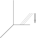
(a)		(b)

Figure 7: (a) For ${\rm C}^{3}$, the 1-cycles $\alpha,\beta$, and $-\alpha-\beta$ of the $T^{2}$ fiber degenerate along the right, upper, and lower-left edges. There are $P$ D-branes on the upper edge. We impose the asymptotic boundary condition the gauge fields on the branes, and it picks out the configuration ${\rm F1}_{R}$ of fundamental strings ending on the branes along the 1-cycle $\alpha$. (b) The boundary condition is also consistent with the branes on the right edge with holonomy $\widehat{U}_{R}$.

We place $P$ non-compact D-branes on the upper edge. The world-volume has topology ${\rm R}^{2}\times S^{1}$, which we regard as solid torus. Since the world-volume has a boundary, we need to impose a boundary condition on the gauge fields on the branes. The boundary condition is a state in the Hilbert space of the Chern-Simons theory on $T^{2}$, and the D-brane amplitude is a wave function. Let us canonically quantize the theory by taking $\oint_{\alpha}A$ as coordinates and $\oint_{\beta}A$ as conjugate momenta. We denote by $(\alpha,\beta)$ the polarization (choice of conjugate variables), which is equivalent to the framing specified by the horizontal arrow in figure 7a [24]. As a basis of the Hilbert space let us take the coordinate eigenstates ${}_{(\alpha,\beta)}\langle V|$ such that

$${}_{(\alpha,\beta)}\langle V|{\rm P}e^{-\oint_{\alpha}A}={}_{(\alpha,\beta)}\langle V|V,$$ (4.13)

where $V$ is a $P\times P$ matrix. The D-brane amplitude $Z_{(\alpha,\beta)}(V)$ is the wave function

$$Z_{(\alpha,\beta)}(V)={}_{(\alpha,\beta)}\langle V|Z\rangle,$$ (4.14)

where $|Z\rangle$ is the state in the Hilbert space intrinsically defined by topological string theory in the given background. The amplitude $Z^{(\alpha,\beta)}(V)$ is computed by summing over many possible string configurations that end on the D-branes while fixing the background holonomy $V$ along $\alpha$. This is the conventional treatment of non-compact D-branes [30, 24].

Another important basis consists of states ${}_{(\alpha,\beta)}\langle R|$. When the state ${}_{(\alpha,\beta)}\langle R|$ is used as a boundary condition on non-compact branes, it picks out the configuration ${\rm F1}_{R}$ of strings. This is the defining property of the state. The Fourier transform

$$Z_{(\alpha,\beta)}(V)=\sum_{R}{\rm Tr}_{R}V\ Z_{(\alpha,\beta),R}$$ (4.15)

relates the D-brane amplitude $Z_{(\alpha,\beta)}(V)$ to

$$Z_{(\alpha,\beta),R}\equiv{}_{(\alpha,\beta)}\langle R|Z\rangle,$$ (4.16)

which is the partition function of strings in the configuration ${\rm F1}_{R}$ as we defined in section 2.

Suppose we use the state ${}_{(\alpha,\beta)}\langle R|$ as a boundary condition for the $P$ D-branes. It was shown in [31] that ${}_{(\alpha,\beta)}\langle R|$ is in fact a momentum eigenstate:

$${}_{(\alpha,\beta)}\langle R|{\rm P}e^{-\oint_{\beta}A}={}_{(\alpha,\beta)}\langle R|\widehat{U}_{R},~{}~{}~{}\widehat{U}_{R}\equiv{\rm diag}(q^{R_{i}-i+1/2+P/2}).$$ (4.17)

On the upper edge, $\beta$ is a contractible cycle and cannot support a non-trivial holonomy. To interpret the non-trivial holonomy, we note that the cycle $\beta$ is non-contractible on the right edge. Indeed, $(\beta,-\alpha)$ is precisely the polarization for the D-branes on the right edge with framing specified by the vertical arrow as shown in figure 7b. Therefore we have that

$${}_{(\alpha,\beta)}\langle R|\propto{}_{(\beta,-\alpha)}\langle\widehat{U}_{R}|,$$ (4.18)

and the partition function $Z_{(\alpha,\beta),R}$ for strings should be identified with the partition function of the D-branes on the right edge with holonomy $\widehat{U}_{R}$ and the specified framing:

$$Z_{(\alpha,\beta),R}\propto Z_{(\beta,-\alpha)}(\widehat{U}_{R}).$$ (4.19)

This is exactly what we found in section 2, and explains the string/brane transition.

\psfrag{a}{$\alpha$}\psfrag{b}{$\beta$}\psfrag{-a-b}{$-\alpha-\beta$}\includegraphics[scale={.45}]{C3-3.eps}
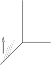
(a)		(b)

Figure 8: (a) The strings extended along the upper edge end on anti-branes along $\alpha$. (b) The boundary condition imposed on the anti-branes that pick out the configuration ${\rm F1}_{R}$ of fundamental strings is equivalent to the condition that the anti-branes end on the lower-left edge with holonomy $\widehat{U}_{R^{T}}\equiv{\rm diag}(q^{R^{T}_{i}-i+1/2+M/2})_{i=1}^{M}$.

We can also understand the transition of strings to anti-branes. Let us begin with the anti-branes with the framing specified by the arrow shown in figure 8a. This framing corresponds to taking $\oint_{\alpha+\beta}A$ and $\oint_{\beta}A$ as canonical coordinates and momenta, respectively. The partition function can be expanded as

$$\overline{Z}_{(\alpha+\beta,\beta)}(V)=\sum_{R}{\rm Tr}_{R}V\ {}_{(\alpha+\beta,\beta)}\langle R|\overline{Z}\rangle.$$ (4.20)

Since anti-branes are related to D-branes by substitution ${\rm Tr}_{R}V\rightarrow(-1)^{|R|}{\rm Tr}_{R^{T}}V$ [24], we have that $|\overline{Z}\rangle=C|Z\rangle$, where $C$ is the charge conjugation operator defined in Appendix B. Thus we find that

$$Z_{(\alpha+\beta,\beta),R} = {}_{(\alpha+\beta,\beta)}\langle R|Z\rangle$$ (4.21)

$$= {}_{(\alpha+\beta,\beta)}\langle R|CC|Z\rangle$$

$$= (-1)^{|R|}{}_{(\alpha+\beta,\beta)}\langle R^{T}|\overline{Z}\rangle$$

$$\propto {}_{(\beta,-\alpha-\beta)}\langle\widehat{U}_{R^{T}}|\overline{Z}\rangle$$

$$= \overline{Z}_{(\beta,-\alpha-\beta)}(\widehat{U}_{R^{T}}).$$

The matrix $\widehat{U}_{R^{T}}$ is the holonomy along $\beta$, which is contractible on the upper edge but non-contractible on the lower-left edge. Moreover, $(\beta,-\alpha-\beta)$ is the polarization for Chern-Simons theory on the anti-branes sitting at the lower-left edge with the framing given by the arrow in figure 8b. This argument implies that $Z_{(\alpha+\beta,\beta),R}$ is proportional to the partition function of the anti-branes with holonomy $\widehat{U}_{R^{T}}$, just as we found in section 2.

Appendix A Unknot Wilson loop vev as a brane amplitude

In this appendix we will rederive the relation between the unknot Wilson loop vev and the partition function of D-branes in the resolved conifold. The original derivation in [15] used a Calabi-Yau crystal in an intermediate step. Here we present a more elementary derivation. We will also formulate a conjecture relating knot polynomials and D-brane amplitudes for general knots.

For the canonically framed unknot, the normalized vev $W_{R}^{(N)}(q)$ in $U(N)$ Chern-Simons theory is

$$W_{R}^{(N)}(q)=S^{(N)}_{0R}/S^{(N)}_{00}={\rm Tr}_{R}\hskip 2.84526pt{\rm diag}(q^{-i+1/2+N/2})_{i=1}^{N}.$$ (A.22)

We manipulate this expression as

$$\frac{\det_{1\leq i,j\leq N}(q^{(-i+1/2+N/2)(R_{j}-j+N)})}{\det_{1\leq i,j\leq N}(q^{(-i+1/2+N/2)(-j+N)})}$$

$$= q^{-\frac{1}{2}(N-1)|R|}\frac{\det_{1\leq i,j\leq N}(q^{(-i+N)(R_{j}-j+N)})}{\det_{1\leq i,j\leq N}(q^{(-i+N)(-j+N)})}$$

$$= q^{-\frac{1}{2}(N-1)|R|}\frac{\prod_{i<j\leq N}\left(q^{R_{i}-i+N}-q^{R_{j}-j+N}\right)}{\prod_{i<j\leq N}\left(q^{-i+N}-q^{-j+N}\right)}$$

$$= q^{\sum_{j}(j-\frac{1}{2}-\frac{1}{2}N)R_{j}}\prod_{i<j\leq N}\frac{1-q^{j-i+R_{i}-R_{j}}}{1-q^{j-i}}$$ (A.23)

$$= q^{\sum_{j}(j-\frac{1}{2}-\frac{1}{2}N)R_{j}}\prod_{i<j\leq P}\frac{1-q^{j-i+R_{i}-R_{j}}}{1-q^{j-i}}\prod_{i\leq P<j\leq N}\frac{1-q^{j-i+R_{i}}}{1-q^{j-i}}$$

$$= q^{\sum_{j}(j-\frac{1}{2}-\frac{1}{2}N)R_{j}}\left[\prod_{i<j\leq P}(1-q^{j-i+R_{i}-R_{j}})\right]\left[\prod_{i<j\leq P}\frac{1}{1-q^{j-i}}\right]$$

$$~{}~{}~{}\times\left[\prod_{i=1}^{P}\prod_{j=1}^{N-P}(1-q^{P+j-i+R_{i}})\right]\left[\prod_{i=1}^{P}\prod_{j=1}^{N-P}\frac{1}{1-q^{P+j-i}}\right].$$

The annulus diagrams between D-branes $\prod_{i<j\leq P}(1-e^{-(y_{i}-y_{j})})$ contribute the first angular bracket in the last expression. The third represents the D-brane amplitudes:

$$\prod_{i=1}^{P}\prod_{j=1}^{N-P}(1-q^{P+j-i+R_{i}}) = \prod_{i=1}^{P}\prod_{j=1}^{\infty}\frac{1-q^{P+j-i+R_{i}}}{1-q^{N+j-i+R_{i}}}$$ (A.24)

$$= \prod_{i=1}^{P}\exp\sum_{n=1}^{\infty}\frac{e^{-ny_{i}}-e^{-n(\widetilde{t}+y_{i})}}{n[n]}.$$

Here we have defined the shifted Kähler modulus $\widetilde{t}=g_{s}(N-P)$. The product of the second and the fourth brackets in (A.23) is the ratio of closed string amplitudes with different values of moduli:

$$\left[\prod_{i<j\leq P}\frac{1}{1-q^{j-i}}\right]\left[\prod_{i=1}^{P}\prod_{j=1}^{N-P}\frac{1}{1-q^{P+j-i}}\right]=\left[\prod_{j=1}^{P}\frac{1}{(1-q^{j})^{P-j}}\right]\left[\prod_{i=1}^{P}\prod_{j=1}^{N-P}\frac{1}{1-q^{i+j-1}}\right]$$ (A.25)

$$= \left[\prod_{j=1}^{P}\frac{(1-q^{j})^{j}}{(1-q^{j})^{P}}\right]\left[\prod_{i=1}^{\infty}\prod_{j=1}^{\infty}\frac{1-q^{P+i+j-1}}{1-q^{i+j-1}}\frac{1-q^{N-P+i+j-1}}{1-q^{N+i+j-1}}\right]$$

$$= \left[\prod_{j=1}^{\infty}\frac{(1-q^{j})^{j}(1-q^{P+j})^{P}}{(1-q^{j})^{P}(1-q^{P+j})^{P+j}}\right]\left[\prod_{j=1}^{\infty}\frac{(1-q^{P+j})^{j}(1-q^{N-P+j})^{j}}{(1-q^{j})^{j}(1-q^{N+j})^{j}}\right]$$

$$= \xi(q)^{P}\prod_{j=1}^{\infty}\frac{(1-q^{N-P+j})^{j}}{(1-q^{N+j})^{j}}=\xi(q)^{P}\exp\left(\sum_{n=1}^{\infty}\frac{e^{-nt}}{n[n]^{2}}-\sum_{n=1}^{\infty}\frac{e^{-n\widetilde{t}}}{n[n]^{2}}\right).$$

To summarize, we have found that

$$\left[\exp-\sum_{n=1}^{\infty}\frac{e^{-nt}}{n[n]^{2}}\right]W^{(N)}_{R}(q)=\left[q^{\sum_{j}(j-\frac{1}{2}-\frac{1}{2}N)R_{j}}\xi(q)^{P}\prod_{i<j\leq P}(1-e^{-(y_{i}-y_{j})})\right]$$

$$\times\left[\prod_{i=1}^{P}\exp\sum_{n=1}^{\infty}\frac{e^{-ny_{i}}-e^{-n(\widetilde{t}+y_{i})}}{n[n]}\right]\left[\exp-\sum_{n=1}^{\infty}\frac{e^{-n\widetilde{t}}}{n[n]^{2}}\right].$$ (A.26)

Let us express (A.26) in a new form, where the precise expression of the D-brane amplitude does not appear. We define the generating functionals, or Fourier transforms, of Wilson loop vevs [30]:

$$G_{+}^{(N)}(q,V) := \sum_{R}W^{(N)}_{R}(q){\rm Tr}_{R}V,$$ (A.27)

$$G_{-}^{(N)}(q,V) := \sum_{R}W^{(N)}_{R}(q)(-1)^{|R|}{\rm Tr}_{R^{T}}V.$$ (A.28)

For the unknot we have

$$G_{\pm}^{(N)}(q,V)=\prod_{i=1}^{N}\det(1-q^{i-(N+1)/2}V)^{\mp 1}=\exp\left(\pm\sum_{n=1}^{\infty}\frac{e^{\frac{1}{2}g_{s}N}-e^{-\frac{1}{2}g_{s}N}}{n[n]}\right){\rm Tr}V^{n}.$$ (A.29)

Thus (A.26) can be written as

$$W^{(N)}_{R}(q)=N_{R}\ G_{+}^{(N-P)}(q,e^{-\widetilde{t}/2}U_{R}),$$ (A.30)

where we have defined the knot-independent factor

$$N_{R}\equiv q^{\sum_{j}(j-\frac{1}{2}-\frac{1}{2}N)R_{j}}\xi(q)^{P}\left[\prod_{i<j\leq P}(1-e^{-(y_{i}-y_{j})})\right]\exp\left(\sum_{n=1}^{\infty}\frac{e^{-n\widetilde{t}}-e^{-nt}}{n[n]^{2}}\right).$$ (A.31)

Up to $N_{R}$, (A.30) tells us that the unknot Wilson loop vev is the Fourier transform of its own. The RHS depends on $R$ almost exclusively through $e^{-y_{i}}$, just like it depends on $N$ only through $e^{-t}$ and $e^{-\widetilde{t}}$. Though we derived (A.30) for the unknot, we conjecture that the relation between the knot polynomials $W_{R}(q,\lambda)\equiv W^{(N)}_{R}(q)$ (here $\lambda=q^{N}$) and their generating functional($=$ D-brane partition function) $G_{+}(q,\lambda,V)\equiv G_{+}^{(N)}(q,V)$ should hold more generally for any knot with a universal normalization factor $N_{R}$. It would be interesting to check the conjecture for torus knots, together with the corresponding relation involving $G_{-}$. The results for torus knots in [32] may be useful.

To rewrite (A.30) in the form of (3.11), note that the Chern-Simons partition function can be identified with the resolved conifold partition function [16]:

$$S_{00}^{(N)}=\left(\frac{g_{s}}{2\pi}\right)^{N/2}e^{-\frac{\pi i}{4}N^{2}}q^{-N(N-1)/12}\xi(q)^{-N}M(q)\exp\left(-\sum_{n}\frac{e^{-nt}}{n[n]^{2}}\right).$$ (A.32)

For precise equality, we should multiply the RHS of (3.11) by the prefactor that contains genus-zero and -one contributions:

$$\left(\frac{g_{s}}{2\pi}\right)^{P/2}e^{-({N^{2}-(N-P)^{2}})\frac{1}{4}\pi i}q^{\sum_{j}(j-\frac{1}{2}-\frac{N}{2})R_{j}-\frac{N(N-1)}{12}+\frac{(N-P)(N-P-1)}{12}}.$$ (A.33)

As is often the case for low-genus contributions, the topological string interpretation of this prefactor is not clear.

Appendix B Operator formalism

Let us review the relation between the representation theory of $U(N)$ and two dimensional bosons and fermions in two dimensions. The formalism is useful in deriving the group theory identities in the main text and dealing with canonical quantization of Chern-Simons theory on $T^{2}$.

Let us consider the mode expansion of a chiral boson $\phi(z)$ and fermions $\psi(z),\overline{\psi}(z)$ in two dimensions, which are related by bosonization:

$$\phi(z)=i\sum_{n\neq 0}\frac{\alpha_{n}}{nz^{n}},~{}~{}\psi(z)=\sum_{r\in{\bf Z}+\frac{1}{2}}\frac{\psi_{r}}{z^{r+1/2}},~{}~{}\overline{\psi}(z)=\sum_{r\in{\bf Z}+\frac{1}{2}}\frac{\overline{\psi}_{r}}{z^{r+1/2}},$$ (B.34)

$$i\partial\phi=:\psi\overline{\psi}:,~{}~{}\psi=:e^{i\phi}:,~{}~{}\overline{\psi}=:e^{-i\phi}:.$$ (B.35)

The oscillator modes satisfy the commutation relations:

$$[\alpha_{n},\alpha_{m}]=n\delta_{n+m,0}\qquad\{\psi_{r},{\overline{\psi}_{s}}\}=\delta_{r+s,0}.$$ (B.36)

We can also define a charge conjugation operator $C$. It exchanges $\psi$ and $\overline{\psi}$:

$$C\psi(z)C=\overline{\psi}(z),~{}C^{2}=1,~{}C|0\rangle=|0\rangle.$$ (B.37)

Then $C$ acts on $i\partial\phi(z)=:\psi(z)\overline{\psi}(z):$ as:

$$C\partial\phi(z)C=-\partial\phi(z).$$ (B.38)

The connection between Young tableau $R$ and fermions arises from the identification

$$|R\rangle=\prod_{i=1}^{d}\psi_{-a_{i}-1/2}\overline{\psi}_{-b_{i}-1/2}|0\rangle,$$ (B.39)

where $a_{i}\equiv R_{i}-i$, $b_{i}=R_{i}^{T}-i$ are the Frobenius coordinates of $R$, and $d$ is the number of boxes in the diagonal of the Young tableau $R$. It follows that:

$$C|R\rangle=(-1)^{|R|}|R^{T}\rangle.$$ (B.40)

Let us now define [33] the operator

$$\Gamma_{\pm}(z):=\exp\sum_{n=1}^{\infty}\frac{z^{\pm n}}{n}\alpha_{\pm n},$$ (B.41)

which satisfies the relations

$$\Gamma_{+}(z_{+})\Gamma_{-}(z_{-})=\frac{1}{1-z_{+}/z_{-}}\Gamma_{-}(z_{-})\Gamma_{+}(z_{+}),~{}~{}\Gamma_{+}(z)|0\rangle=|0\rangle,~{}\langle 0|\Gamma_{-}(z)=\langle 0|.$$ (B.42)

The skew Schur polynomials can be conveniently expressed as

$$s_{R/Q}(x)=\langle R|\prod_{i}\Gamma_{-}(x_{i}^{-1})|Q\rangle=\langle Q|\prod_{i}\Gamma_{+}(x_{i})|R\rangle.$$ (B.43)

The familiar Schur polynomials $s_{R}(x)\equiv{\rm Tr}_{R}{\rm diag}(x_{i})$ arise when $|Q\rangle=|0\rangle$. In terms of the Schur polynomials, the skew Schur polynomials are given by

$$s_{R/Q}(x)=\sum_{R^{\prime}}N^{R}_{QR^{\prime}}s_{R^{\prime}}(x),$$ (B.44)

where $N^{R}_{QR^{\prime}}$ are the Littlewood-Richardson coefficients.

Appendix C Topological vertex amplitude

We use the convention such that $q$ is replaced by $q^{-1}$ relative to [24]. Explicitly the topological vertex amplitude is given, with slight abuse of notation, by:

$$C_{R_{1}R_{2}R_{3}}(q)=q^{-\frac{1}{2}(\kappa_{R_{2}}+\kappa_{R_{3}})}s_{{R_{2}}^{T}}(q^{i-1/2})\sum_{Q}s_{R_{1}/Q}(q^{-(R_{2}^{T})_{i}+i-1/2})s_{{R_{3}}^{T}/Q}(q^{-(R_{2})_{i}+i-1/2}).$$ (C.45)

Here $s_{R_{1}/R_{2}}$ is a skew Schur function. The index $i$ runs from $1$ to $\infty$.

In the next appendix, we need the crystal representation of the topological vertex. This is obtained by a simple manipulation of the results in [33]:

$$C_{R_{1}R_{2}R_{3}}=M(q)^{-1}q^{-\frac{1}{2}\kappa_{R_{1}}+\frac{1}{2}||R^{T}_{3}||^{2}}\left\langle R_{2}\right|\left[\prod_{i=1}^{\infty}\Gamma_{\pm}(q^{i-1/2})\right]\left[\prod_{i=1}^{\infty}\Gamma_{\pm}(q^{-i+1/2})\right]\left|R_{1}{}^{T}\right\rangle.$$ (C.46)

In this expression, the pattern of $\Gamma_{\pm}$ is determined by $R_{3}$ as described in [33], and the border between the two products is the diagonal of $R_{3}$.

The partition function of topological strings on any toric Calabi-Yau manifold, with or without $D$-branes, can be computed by gluing several topological vertices. The gluing rules are explained in [24].

Appendix D An identity for string/brane transitions

The aim of this appendix is to prove the identity (2.7).

$$\sum_{Q_{2},Q_{2}^{\prime}}C_{\cdot Q_{2}R_{3}}(-1)^{|Q_{2}|}q^{\frac{1}{2}\kappa_{Q_{2}}}{\rm Tr}_{Q_{2}/Q_{2}^{\prime}}U_{R}(-1)^{|Q_{2}^{\prime}|}{\rm Tr}_{R_{2}{}^{T}/Q_{2}^{\prime}{}^{T}}U_{R}{}^{-1}$$

$$= \sum_{Q_{2},Q_{2}^{\prime}}\langle R_{3}\left[\prod_{i=1}^{\infty}\Gamma_{-}(q^{-i+1/2})\right]\left[\prod_{i=1}^{\infty}\Gamma_{+}(q^{i-1/2})\right]|Q_{2}{}^{T}\rangle(-1)^{|Q_{2}|}\langle Q_{2}|$$

$$\times\left[\prod_{i=1}^{P}\Gamma_{-}(q^{-R_{i}+i-P-1/2})\right]|Q_{2}^{\prime}\rangle(-1)^{|Q_{2}^{\prime}|}\langle Q_{2}^{\prime}{}^{T}|\left[\prod_{i=1}^{P}\Gamma_{+}(q^{-R_{i}+i-P-1/2})\right]|R_{2}{}^{T}\rangle$$

$$= \langle R_{3}|\left[\prod_{i=1}^{\infty}\Gamma_{-}(q^{-i+1/2})\right]\left[\prod_{i=1}^{\infty}\Gamma_{+}(q^{i-1/2})\right]$$

$$\times C\left[\prod_{i=1}^{P}\Gamma_{-}(q^{-R_{i}+i-P-1/2})\right]C\left[\prod_{i=1}^{P}\Gamma_{+}(q^{-R_{i}+i-P-1/2})\right]|R_{2}{}^{T}\rangle$$

$$= \langle R_{3}|\left[\prod_{i=1}^{\infty}\Gamma_{-}(q^{-i+1/2})\right]\left[\prod_{i=1}^{\infty}\Gamma_{+}(q^{i-1/2})\right]$$ (D.47)

$$\times\left[\prod_{i=1}^{P}\Gamma_{-}^{-1}(q^{-R_{i}+i-P-1/2})\right]\left[\prod_{i=1}^{P}\Gamma_{+}(q^{-R_{i}+i-P-1/2})\right]|R_{2}{}^{T}\rangle$$

$$= \langle R_{3}|\left[\prod_{i=1}^{\infty}\Gamma_{+}(q^{i-1/2})\right]\left[\prod_{i=1}^{\rightarrow\infty}\Gamma_{-}(q^{-i+1/2})\right]\left[\prod_{i=1}^{P\leftarrow}\Gamma_{-}^{-1}(q^{-R_{i}+i-P-1/2})\Gamma_{+}(q^{-R_{i}+i-P-1/2})\right]$$

$$\times|R_{2}{}^{T}\rangle M(q)^{-1}\prod_{i=1}^{P}\prod_{j=1}^{i-1}(1-q^{-R_{i}+i+R_{j}-j})^{-1}$$

$$= \langle R_{3}|\left[\prod_{i=1}^{\infty}\Gamma_{\pm}(q^{i-1/2})\right]\left[\prod_{i=1}^{\rightarrow\infty}\Gamma_{\mp}(q^{-i+1/2})\right]|R_{2}{}^{T}\rangle$$

$$\times q^{P|R_{3}|-P|R_{2}|}M(q)^{-1}\prod_{i=1}^{P}\prod_{j=1}^{i-1}(1-q^{-R_{i}+i+R_{j}-j})^{-1}\left(\prod_{j=1}^{\infty}(1-q^{j})\right)^{P}$$

$$= \xi(q)^{-P}\prod_{1\leq i<j\leq P}(1-e^{-(a_{i}-a_{j})})^{-1}C_{RR_{2}R_{3}}q^{\frac{1}{2}\kappa_{R_{2}}-\frac{1}{2}||R^{T}||^{2}}q^{P|R_{3}|-P|R_{2}|}.$$

Here we used the crystal representation (C.46) of the topological vertex. The arrows above the product symbols indicate the direction we order the factors.

References

• [1] J. M. Maldacena, “The large N limit of superconformal field theories and supergravity,” Adv. Theor. Math. Phys. 2 (1998) 231–252, hep-th/9711200.
• [2] A. Strominger and C. Vafa, “Microscopic Origin of the Bekenstein-Hawking Entropy,” Phys. Lett. B379 (1996) 99–104, hep-th/9601029.
• [3] R. Dijkgraaf and C. Vafa, “Matrix models, topological strings, and supersymmetric gauge theories,” Nucl. Phys. B644 (2002) 3–20, hep-th/0206255.
• [4] R. Dijkgraaf and C. Vafa, “A perturbative window into non-perturbative physics,” hep-th/0208048.
• [5] J. Callan, Curtis G. and J. M. Maldacena, “Brane dynamics from the Born-Infeld action,” Nucl. Phys. B513 (1998) 198–212, hep-th/9708147.
• [6] G. W. Gibbons, “Born-Infeld particles and Dirichlet p-branes,” Nucl. Phys. B514 (1998) 603–639, hep-th/9709027.
• [7] J. McGreevy, L. Susskind, and N. Toumbas, “Invasion of the giant gravitons from anti-de Sitter space,” JHEP 06 (2000) 008, hep-th/0003075.
• [8] M. T. Grisaru, R. C. Myers, and O. Tafjord, “SUSY and Goliath,” JHEP 08 (2000) 040, hep-th/0008015.
• [9] A. Hashimoto, S. Hirano, and N. Itzhaki, “Large branes in AdS and their field theory dual,” JHEP 08 (2000) 051, hep-th/0008016.
• [10] J. M. Maldacena, “Wilson loops in large N field theories,” Phys. Rev. Lett. 80 (1998) 4859–4862, hep-th/9803002.
• [11] N. Drukker and B. Fiol, “All-genus calculation of Wilson loops using D-branes,” JHEP 02 (2005) 010, hep-th/0501109.
• [12] S. Yamaguchi, “Wilson loops of anti-symmetric representation and D5-branes,” JHEP 05 (2006) 037, hep-th/0603208.
• [13] J. Gomis and F. Passerini, “Holographic Wilson loops,” hep-th/0604007.
• [14] J. Gomis and F. Passerini, “Wilson loops as D3-branes,” hep-th/0612022.
• [15] J. Gomis and T. Okuda, “Wilson loops, geometric transitions and bubbling Calabi- Yau’s,” JHEP 02 (2007) 083, hep-th/0612190.
• [16] R. Gopakumar and C. Vafa, “On the gauge theory/geometry correspondence,” Adv. Theor. Math. Phys. 3 (1999) 1415–1443, hep-th/9811131.
• [17] J. Gomis and T. Okuda, “D-branes as a Bubbling Calabi-Yau,” arXiv:0704.3080 [hep-th].
• [18] V. Balasubramanian, M. Berkooz, A. Naqvi, and M. J. Strassler, “Giant gravitons in conformal field theory,” JHEP 04 (2002) 034, hep-th/0107119.
• [19] S. Corley, A. Jevicki, and S. Ramgoolam, “Exact correlators of giant gravitons from dual N = 4 SYM theory,” Adv. Theor. Math. Phys. 5 (2002) 809–839, hep-th/0111222.
• [20] H. Lin, O. Lunin, and J. M. Maldacena, “Bubbling AdS space and 1/2 BPS geometries,” JHEP 10 (2004) 025, hep-th/0409174.
• [21] S. Yamaguchi, “Bubbling geometries for half BPS Wilson lines,” hep-th/0601089.
• [22] O. Lunin, “On gravitational description of Wilson lines,” JHEP 06 (2006) 026, hep-th/0604133.
• [23] M. Aganagic, R. Dijkgraaf, A. Klemm, M. Marino, and C. Vafa, “Topological strings and integrable hierarchies,” Commun. Math. Phys. 261 (2006) 451–516, hep-th/0312085.
• [24] M. Aganagic, A. Klemm, M. Marino, and C. Vafa, “The topological vertex,” Commun. Math. Phys. 254 (2005) 425–478, hep-th/0305132.
• [25] M. Aganagic, M. Marino, and C. Vafa, “All loop topological string amplitudes from Chern-Simons theory,” Commun. Math. Phys. 247 (2004) 467–512, hep-th/0206164.
• [26] N. Saulina and C. Vafa, “D-branes as defects in the Calabi-Yau crystal,” hep-th/0404246.
• [27] T. Okuda, “Derivation of Calabi-Yau crystals from Chern-Simons gauge theory,” JHEP 03 (2005) 047, hep-th/0409270.
• [28] M. Marino, “Chern-Simons theory, matrix models, and topological strings,”. Oxford, UK: Clarendon (2005) 197 p.
• [29] D.-E. Diaconescu, B. Florea, and A. Grassi, “Geometric transitions and open string instantons,” Adv. Theor. Math. Phys. 6 (2003) 619–642, hep-th/0205234.
• [30] H. Ooguri and C. Vafa, “Knot invariants and topological strings,” Nucl. Phys. B577 (2000) 419–438, hep-th/9912123.
• [31] S. Elitzur, G. W. Moore, A. Schwimmer, and N. Seiberg, “Remarks on the canonical quantization of the Chern-Simons-Witten theory,” Nucl. Phys. B326 (1989) 108.
• [32] J. M. F. Labastida and M. Marino, “Polynomial invariants for torus knots and topological strings,” Commun. Math. Phys. 217 (2001) 423–449, hep-th/0004196.
• [33] A. Okounkov, N. Reshetikhin, and C. Vafa, “Quantum Calabi-Yau and classical crystals,” hep-th/0309208.