Off-center HII regions in power-law density distributions

Abstract

The expansion of ionization fronts in uniform and spherically symmetric power-law density distributions is a well-studied topic. However, in many situations, such as a star formed at the edge of a molecular cloud core, an offset power-law density distribution would be more appropriate. In this paper a few of the main issues of the formation and expansion of HII regions in such media are outlined and results are presented for the particular cases where the underlying power laws are $r^{-2}$ and $r^{-3}$. A simple criterion is developed for determining whether the initial photoionized region will be unbounded, which depends on the power-law exponent and the ratio of the equivalent Strömgren radius produced by the star in a uniform medium to the stellar offset distance. In the expansion stage, the ionized volumes will eventually become unbounded unless pressure balance with the external medium is reached before the ionization front velocity becomes supersonic with respect to the ionized gas.

1. Introduction

The theoretical study of the formation and evolution of H II regions in non uniform media is motivated by the observational result that the molecular clouds where massive star form generally possess density gradients (e.g., Lada et al., 2007). The assumed density law is taken to be a power law $n\propto r^{-\alpha}$ with exponents ranging from 1 to 3 (Arquilla & Goldsmith, 1985) obtained from molecular line studies. Submillimeter continuum dust emission observations of the molecular material around embedded ultracompact H II regions gives an exponent in the range 1.25 to 2.25 (Hatchell & van der Tak, 2003). The most commonly found value for the power-law exponent is $\alpha=2$, which correponds to an isothermal, self-gravitating sphere. However, steeper density laws, $\alpha<4$ have been inferred from radio continuum spectra of a sample of ultracompact H II regions (Franco et al., 2000).

Numerical studies of H II region expansion near the edge of a molecular cloud (the so-called “champagne flows”), were carried out by Tenorio-Tagle and collaborators (Tenorio-Tagle, 1979; Bodenheimer et al., 1979; Bedijn & Tenorio-Tagle, 1981). In this model, an H II region formed near the edge of the cloud “breaks out” into the low density, intercloud medium during the expansion stage and the ionized gas can achieve supersonic velocities of around 30 km s^-1 in the accelerating flow. This problem was studied in more detail by Henney et al. (2005), and applied to the Orion Nebula H II region. They found that a long-lived quasi-stationary phase exists in which the ionized flow is approximately steady in the frame of reference of the ionization front. during this phase, the flow structure is determined entirely by the distance of the ionizing star from the front and the curvature of the front. The curvature determines whether the flows are more “champagne like” or “globule like”. The curvature of the ionization front depends on the lateral density distribution in the neutral gas.

Franco et al. (1989, 1990) developed analytical solutions for the formation and expansion of H II regions in spherically symmetric, power-law density distributions, where the ionizing star is assumed to be at the center of the density distribution. The main result of their paper is that for spherical clouds with power-law density distributions $r^{-\alpha}$, there is a critical value of the exponent, $\alpha_{\rm crit}=3/2$ above which the cloud becomes completely ionized during the expansion phase of the H II region. For power-law exponents higher than this critical value, two regimes were identified: a slow regime, in which the expansion of the dense cloud core is mildly supersonic and has almost constant velocity, corresponding to $3/2<\alpha\leq 3$, and the fast regime, where the core expansion drives a strongly accelerating shock, which corresponds to $\alpha>3$. This problem was revisited by Shu et al. (2002), who developed a self-similar solution for the internal motions in the ionized gas in the $\alpha>3/2$ cases.

Franco et al. (1989, 1990) also considered self-gravitating isothermal disk density distributions where the density fall-off is steeper than $r^{-3/2}$. In this case, the H II region becomes unbounded in a conical section of the disk, where the opening angle of the cone depends on the ratio of the Strömgren radius in the midplane density to the density distribution scale height. During the expansion stage of such H II regions, the flattening of the internal ionized gas density distribution can lead to the trapping of an initially unbounded ionization front.

More recently, photoionized regions in a variety of axisymmetric density distributions were modeled numerically by Arthur & Hoare (2006), who also included the central star’s stellar wind. In that work, it was found that the hot bubble created by the shocked stellar wind results in a champagne flow being set up outside the swept-up stellar wind shell, leading to mixed kinematics from an observational point of view. Arthur & Hoare (2006) also considered the possibility of stellar motion up the density gradient, which introduces the added complication of bowshock kinematics to the problem.

Mac Low et al. (2006) performed low-resolution three-dimensional numerical simulations of H II region dynamical evolution in a collapsing molecular cloud. Here, the density distribution had a core-envelope structure, where the envelope had a power-law ($r^{-2}$) density distribution. Both turbulent and non-turbulent cases were modeled. In the non-turbulent case, even for ionizing sources off-center from the core, the H II region expansion was nearly spherical for the parameters adopted and the timescale of the simulation.

The photoionized regions produced by moving stars were studied numerically by Franco et al. (2007). In that paper, the H II regions produced by a star off-center in a spherically symmetric density distribution were modeled, where a range of stellar velocities (between 0 and 12 km s^-1) were considered. It was found that the H II region produced by a star off-center in an underlying $r^{-2}$ density distribution did not become unbounded, while that in a $r^{-3}$ density distribution did, for the case of a stationary star. This appears to contradict the main result of Franco et al. (1990). This result is the motivation for the present work, where we aim to provide simple tools for analyzing the formation and expansion of H II regions off-center in spherically symmetric density distributions.

The structure of this paper is as follows: in § 2 we outline the problem and discuss the initial formation stage of an H II region off-center in a spherically symmetric density distribution and find a criterion for the H II region to remain bounded. In § 3 we investigate the expansion stage and derive a simple differential equation that describes the expansion of the ionization front along the symmetry axis. We assess the validity of our assumptions about the internal structure of the ionized gas by comparing our analytical model with the results of numerical simulations in § 4. Finally, in § 5 we summarize our results.

2. Description of the problem

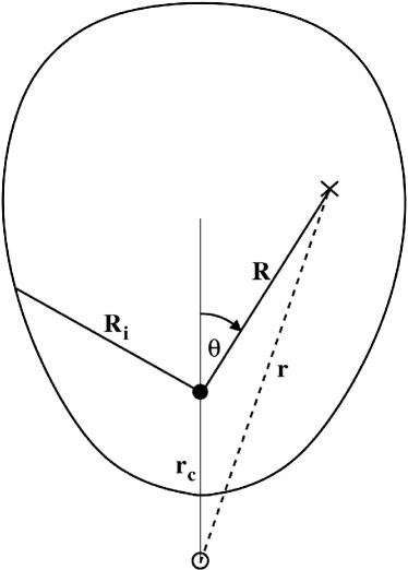
Figure 1.— Geometrical configuration. The center of the (spherically symmetric) power-law density distribution is denoted by the open circle, the star is represented by the filled circle, a distance $r_{c}$ from the density center. For a parcel of gas at X, distance $r$ from the density center, the star-centered coordinates are $(R,\theta)$, where $R$ is the distance from the star and $\theta$ is measured clockwise from the extension of the line joining the star to the density center. Rotational symmetry is assumed around the axis joining the star to the center of the density distribution. The position of the ionization front in this coordinate system is $R_{i}$. An approximate shape for the ionization front is also shown.

The underlying, spherically symmetric density distribution is described by

$$n(r)=n_{c}\left(\frac{r}{r_{c}}\right)^{-\alpha}$$ (1)

where $n_{c}$ is the number density at the position of the star, $r_{c}$. We now change our reference system and rewrite the density distribution in axisymmetric coordinates centered on the star position, with the distance from the star, $R$, found from

$$R^{2}-2r_{c}R\cos(\pi-\theta)+r_{c}^{2}-r^{2}=0\ ,$$ (2)

where $\theta$ is measured from the symmetry axis and the center of the density distribution is in the direction $\theta=\pi$, see Figure 1. The density distribution of Equation 1, in terms of this new reference system, $(R,\theta)$, becomes

$$n(R,\theta)=n_{c}\left(\frac{R^{2}+r_{c}^{2}+2r_{c}R\cos\theta}{r_{c}^{2}}\right)^{-\alpha/2}\ .$$ (3)

Along the symmetry axis, $\theta=0$, this can be written

$$n(y)=n_{c}\left(1+y\right)^{-\alpha}\ ,$$ (4)

where we have defined $y=R/r_{c}$.

For $y<1$, expansion to linear terms in a Taylor series shows that

$$n(y)\approx n_{c}(1-\alpha y)\ ,$$ (5)

which is no longer a power law. For $y>1$ we find $n(y)\approx n_{c}y^{-\alpha}$, that is, the offset density distribution resembles the original power-law density distribution. Consequently, if the initial Strömgren radius, $R_{s}$, is smaller than the stellar offset distance, then we expect the initial H II region to remain confined, even for power laws steeper than $\alpha>3/2$.

2.1. Condition for the initial Strömgren region

We can develop a quantitative criterion for deciding whether the initial photoionized region will remain bounded in an offset power-law density distribution by balancing recombinations and ionizations, assuming pure hydrogen, along the symmetry axis $\theta=0$:

$$\alpha_{B}r_{c}^{3}\int^{y}_{0}n_{c}^{2}\left(1+y^{\prime}\right)^{-2\alpha}y^{\prime 2}\ dy^{\prime}=\frac{Q_{H}}{4\pi}\ ,$$ (6)

where $\alpha_{B}$ is the case B recombination coefficient. This equation can be written

$$\int^{y}_{0}\left(1+y^{\prime}\right)^{-2\alpha}y^{\prime 2}\ dy^{\prime}=\frac{1}{3}y^{3}_{\rm sc}\ ,$$ (7)

where $y_{\rm sc}$ is the non-dimensionalized Strömgren radius for a uniform medium of number density $n_{c}$, i.e.,

$$y_{\rm sc}=\frac{R_{s}}{r_{c}}=\left(\frac{3Q_{H}}{4\pi\alpha_{B}n_{c}^{2}r_{c}}\right)^{1/3}\ .$$ (8)

In the “uphill” direction, $\theta=\pi$, the equivalent non-dimensionalized ionization balance equation is

$$\int^{y}_{0}\left(1-y^{\prime}\right)^{-2\alpha}y^{\prime 2}\ dy^{\prime}=\frac{1}{3}y_{\rm sc}^{3}\ .$$ (9)

Equations 8 and 9 define integral equations for the extent of the ionized region, $y$, along $\theta=0$ and $\theta=\pi$, respectively, as functions of $y_{\rm sc}$ and $\alpha$.

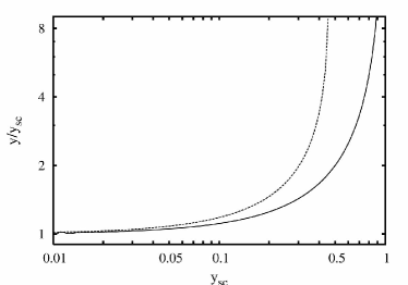
Figure 2.— Ratio of ionization front radius along $\theta=0$ to uniform density Strömgren radius, $y/y_{\rm sc}$, as a function of uniform density Strömgren radius, $y_{\rm sc}$, for power-law density distributions with exponent $\alpha=2$ (solid line) and $\alpha=3$ (dashed line). The asymptotes are $y_{\rm sc}=1$ for $\alpha=2$ and $y_{\rm sc}=0.464$ for $\alpha=3$.

Integrating Equation 7 for $\alpha>3/2$ we obtain

$$\frac{1}{3}y_{\rm sc}^{3}= \frac{-2}{(1-2\alpha)(2-2\alpha)(3-2\alpha)}(1-[1+y]^{3-2\alpha})$$ (10)

$$-\frac{2}{(1-2\alpha)(2-2\alpha)}(y[1+y]^{2-2\alpha})$$

$$+\frac{1}{(1-2\alpha)}(y^{2}[1+y]^{1-2\alpha})\ .$$

In general, this yields a positive, real root for $y$ (the non-dimensionalized ionization front radius) as long as

$$\frac{1}{3}y_{\rm sc}^{3}<\frac{2}{(2\alpha-1)(2\alpha-2)(2\alpha-3)}\ .$$ (11)

For example, when $\alpha=2$, the requirement is $y_{\rm sc}<1$, while for $\alpha=3$, the condition is $y^{3}_{\rm sc}<0.1$, i.e., $y_{\rm sc}<0.464$, in order that there be a real, positive root for $y$. In Figure 2 we plot the ratio $y/y_{\rm sc}$ against $y_{\rm sc}$ for $y_{\rm sc}$ values between 0.01 and 1.0 for the two examples above, $\alpha=2$ and $\alpha=3$. We see that for $y_{\rm sc}$ less than the critical value, the value of the root $y$ is not too different from $y_{\rm sc}$, but close to the critical value $y/y_{\rm sc}\rightarrow\infty$.

3. Expansion stage

In order to study the expansion of the ionized gas after the initial formation of the photoionized region we follow the same analysis as Spitzer (1968) and Shu (1992). As the H II region expands, a neutral shock is sent out ahead of the ionization front into the ambient medium.

Across the isothermal shock, the relevant equations are mass conservation

$$\rho_{1s}v_{1s}=\rho_{2s}v_{2s}\ ,$$ (12)

and momentum conservation

$$p_{1s}+\rho_{1s}v_{1s}^{2}=p_{2s}+\rho_{2s}v_{2s}^{2}$$ (13)

where the subscript $1s$ refers to preshock conditions and $2s$ refers to postshock conditions and all velocities are in the frame of the shock. We also have the equation for the density jump across a weak-D ionization front

$$\frac{\rho_{2i}}{\rho_{1i}}=\frac{1}{2c_{2}^{2}}\left\{\left(c_{1}^{2}+v_{1i}^{2}\right)^{2}+\left[\left(c_{1}^{2}+v_{1i}^{2}\right)^{2}-4c_{2}^{2}v_{1i}^{2}\right]^{1/2}\right\}$$ (14)

where the subscript $1i$ refers to conditions conditions in front of the ionization front and $2i$ refers to conditions in the photoionized gas just behind the ionization front. Here, $c_{1}$ is the sound speed in the neutral gas and $c_{2}$ is the sound speed in the ionized gas, and $v_{1i}$ refers to the velocity of the gas ahead of the ionization front in the frame of the ionization front.

Furthermore, we assume that the region between the shock front and the ionization front is thin, i.e. $u_{1i}=u_{2s}$, where $u_{1i}$ and $u_{2s}$ are the velocities of the gas ahead of the ionization front and behind the shock front in the frame of the star, and that the density of the ionized gas inside the photoionized region is spatially uniform but decreases with time, i.e. $\rho_{2i}\equiv\rho_{2i}(t)$. This is valid if the sound-crossing time of the ionized region is short compared to the expansion timescale.

As a first approximation to the non-spherical shape of the ionization front in a non-uniform density distribution, we assume that the radius of the ionization front can be described by

$$R_{i}=a_{0}+a_{1}\cos\theta\equiv a_{0}+a_{1}\mu$$ (15)

to first order in $\mu=\cos\theta$, where

$$a_{0}=\frac{R_{-}+R_{+}}{2}$$ (16)

and

$$a_{1}=\frac{R_{-}-R_{+}}{2}$$ (17)

with $R_{-}$ corresponding to the shell radius when $\mu=-1$ and $R_{+}$ to the case $\mu=1$ (see, e.g., Dyson, 1977).

The volume contained within the ionization front $R_{i}$ is

$$V_{i}=\frac{2\pi}{3}\int_{-1}^{1}R(\mu)^{3}\ d\mu\ ,$$ (18)

which in this approximation becomes

$$V_{i}=a_{0}^{3}\left(1+\frac{a_{1}^{2}}{a_{0}^{2}}\right)\ .$$ (19)

Assuming uniform expansion, then the mass contained within a volume, $V$, interior to an internal shell of radius $R$ must be conserved during the expansion. That is,

$$\rho_{2i}V=\mbox{constant}\ ,$$ (20)

and the total volume of ionized gas satisifies the ionization balance equation, where the ionizing photon output of the star is assumed to be constant, that is

$$\rho_{2i}^{2}V_{i}=\mbox{constant}\ .$$ (21)

Taking the time derivatives of Equations 20 and 21 we find that

$$\left.\frac{dV}{dt}\right|_{R_{i}}=\frac{1}{2}\frac{dV_{i}}{dt}\ .$$ (22)

where we have evaluated the derivative for a shell located just inside the ionization front radius. Writing

$$\frac{dV}{dt}=\frac{dV}{dR}\frac{dR}{dt}\mbox{\hskip 20.00003pt and \hskip 20.00003pt}\frac{dV_{i}}{dt}=\frac{dV_{i}}{dR_{i}}\frac{dR_{i}}{dt}$$ (23)

then we find that the gas velocity behind the ionization front is half the ionization front velocity, $u_{2i}=0.5U_{i}$, where $u_{2i}=\left.\frac{dR}{dt}\right|_{R_{i}}$ and $U_{i}=\frac{dR_{i}}{dt}$. This assumes that the expansion is uniform and that there are no lateral gas motions within the photoionized region.

With the additional assumption that $v_{1i}/{c_{1}}\ll 1$, then equations 12, 13, 14, together with $u_{2i}=0.5U_{i}$, can be combined to give

$$\frac{\rho_{2i}}{\rho_{1s}}=\frac{4U_{i}^{2}}{4c_{2}^{2}+U_{i}^{2}}\ ,$$ (24)

where we have used the thin shell approximation $U_{i}\approx U_{s}$. These assumptions are the same as those of Spitzer (1968).

The density ratio can be found from ionization balance

$$\rho_{2i}^{2}V_{i}=\rho_{c}^{2}R_{0}^{3}\ ,$$ (25)

where $R_{0}$ is the initial Strömgren radius formed in a medium of uniform mass density $\rho_{c}$. We also have the offset power-law initial density distribution, written here for $\mu\pm 1$:

$$\rho_{1s}=\rho_{c}\left(1\pm\frac{R}{r_{c}}\right)^{-\alpha}\ ,$$ (26)

where $r_{c}$ is the offset distance of the star from the center of the density distribution and $\rho_{c}$ is the density at this point. Thus

$$\frac{\rho_{2i}}{\rho_{1s}}=\left(\frac{R_{0}^{3}}{V_{i}}\right)^{1/2}\left(1\pm\frac{R}{r_{c}}\right)^{\alpha}\$$ (27)

in the directions $\mu=\pm 1$ along the symmetry axis.

Equation 24 can be written in the form

$$M^{2}\left(4-\frac{\rho_{2i}}{\rho_{1s}}\right)=4\frac{\rho_{2i}}{\rho_{1s}}\ ,$$ (28)

where $M=U_{i}/c_{2}$. This constitutes a differential equation for the radius of the ionization front, $R_{i}$, as a function of time and can be solved numerically with standard techniques (e.g., Press et al., 1992), by considering directions $\mu=1$ and $\mu=-1$ together and using equations 15, 16, 17, 18 and 27, with initial conditions $M=2/\sqrt{3}$ when $t=0$, $R_{i}=R_{0}$ and $\rho_{2i}=\rho_{1s}$. Here, it is assumed that $R_{0}$ is much less than the critical value found from solving Equation 11 above, and so the initial ionized region radius ($R_{i}$ at $t=0$) is taken to be that for a uniform medium.

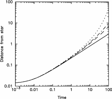
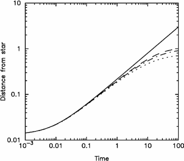
Figure 3.— Radius of the ionization front (in units of the stellar offset radius, $r_{c}$) against time (in units of the sound crossing time, $\tau=r_{c}/c_{2}$). Top: $\mu=1$ direction. Bottom: $\mu=-1$ direction. Density power laws are $\alpha=0$ (solid line), $\alpha=3/2$ (dashed line), $\alpha=2$ (dot-dashed line), and $\alpha=3$ (dotted line).

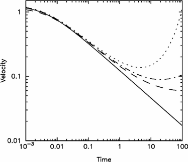
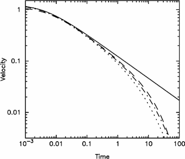
Figure 4.— Velocity of the ionization front (in units of the ionized gas sound speed) against time (in units of the sound crossing time). Top: $\mu=1$ direction. Bottom: $\mu=-1$ direction. Linetypes same as in Fig. 3.

In Figures 3 and 4 we can see the result of solving Equation 28 numerically for the cases $\alpha=0$, 2 and 3. In these figures, all distances are scaled to $r_{c}$ and times are scaled with the sound crossing time of this distance in the ionized gas, $\tau=r_{c}/c_{2}$. The results presented are particular to the case $y_{\rm sc}=R_{0}/r_{c}=0.01324$, which corresponds to an ionizing source with $Q_{H}=10^{48}$ photons s^-1 and a density $n_{c}=10^{7}/e$ cm^-3, where we have also assumed that the case B recombination coefficient takes the value $\alpha_{B}=2.6\times 10^{-13}$ cm³ s^-1. These values of the parameters are motivated by Franco et al. (2007).

In the “upward” direction ($\mu=-1$, density increasing), as expected the radius grows more slowly in the $\alpha=2$ and $3$ cases than for the uniform medium, classical case $\alpha=0$, as shown in Figures 3 and 4. In the “downward” direction, $\mu=1$, Figures 3 and 4 clearly show that in the $\alpha=3$ case, the velocity starts to increase after about 5 sound crossing times and by 100 sound crossing times the velocity of the ionization front has become supersonic with respect to the ionized gas. This means that the ionization front has overtaken the shock wave and will ionize out to infinity. In the $\alpha=2$ case, although the velocity does start to increase again after about 13 sound crossing times, the increase is only very gradual, and within the timescale studied the ionization front does not become supersonic with respect to the ionized gas.

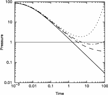
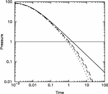
Figure 5.— Internal to external pressure ratio against time (in units of the sound crossing time). Top: $\mu=1$ direction. Bottom: $\mu=-1$ direction. Linetypes same as in Fig. 3. The horizontal line marks equal pressures.

In Figure 5 we show the ratio of the pressure in the ionized gas to that in the ambient medium, assuming that the latter is isothermal with a temperature of 100 K. From these figures we see that in the $\mu=-1$ direction the pressures equalize in about 1 sound crossing time for both $\alpha=2$ and $\alpha=3$. In the $\mu=1$ direction, the $\alpha=3$ case shows that the pressures do not equalize before the ionization front begins to accelerate. In the $\alpha=2$ case, the pressures do equalize at around 7 sound crossing times for the adopted parameters (i.e., initial Strömgren radius, $R_{0}$). We remark that once the pressures become similar, the analysis of this section does not really hold, since the external pressure should be taken into account. However, we also comment that the fact that the pressures do become equal before the shock begins to accelerate in the $\alpha=2$ case means that, in practice, the H II region will remain confined for this choice of initial Strömgren radius.

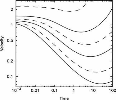
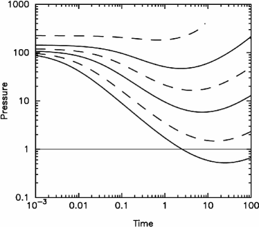
Figure 6.— Top: Velocity of the ionization front (in units of the ionized gas sound speed) against time (in units of the sound crossing time) for different values of the initial Strömgren radius. From lowest line to uppermost line: $R_{0}/r_{c}=0.01$, 0.02, 0.05, 0.1, 0.2, 0.5. Bottom: Ratio of internal to external pressures for the same initial Strömgren radius values. The horizontal line denotes equal pressures.

In Figure 6 we show how the breakout time of the ionization front in the $\mu=1$ direction varies with initial Strömgren radius, for values of $R_{0}/r_{c}$ between 0.01 and 1.0 for the case $\alpha=2$. As $R_{0}/r_{c}\rightarrow 1$ the position of the velocity minimum moves to earlier times and higher velocities. Also in this figure, we show how the internal to external pressure ratio varies with initial Strömgren radius. Only for $R_{0}/r_{c}\lesssim 0.02$ is there a regime for which pressure balance could possibly halt the expansion and subsequent breakout of the H II region.

4. Numerical Simulation

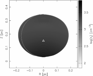
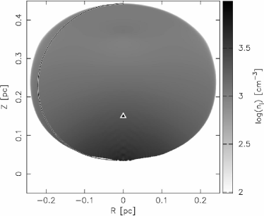
Figure 7.— Logarithm of ionized gas density. Top: $\alpha=2$ numerical solution after 60,000 yrs. Bottom: $\alpha=3$ numerical solution after 50,000 yrs. The black triangle marks the position of the star and the position $(0,0)$ denotes the center of the density distribution in each case. The heavy black curve represents the shape of the ionization front obtained from the approximation of Equation 15.

In order to test our assumption that the density within the ionized gas is approximately constant during the expansion stage, we perform numerical simulations of the expansion of an off-center H II region in a power-law density distribution. The density law for this simulation is taken from Franco et al. (2007), namely

$$n(r)=\left\{\begin{array}[]{ll}n_{0}\exp\left[-\frac{\alpha}{2}\left(r/r_{c}\right)^{2}\right]&\mbox{for $r\leq r_{c}$},\\ n_{0}e^{-\alpha/2}\left(r/r_{c}\right)^{-\alpha}&\mbox{for $r\geq r_{c}$},\end{array}\right.$$ (29)

where $n_{0}$ is the central density and $r_{c}$ is the stellar offset distance from the center of the density distribution. At $r_{c}$ the density has the value $n_{c}\equiv n(r_{c})=n_{0}/e^{\alpha/2}$.

This density distribution is flatter for radii $r<r_{c}$ than the simple power-law density distribution discussed in §§ 2 and 3 above. It is obtained by assuming that the acceleration due to gravity of the hydrostatic equilbrium solution in the halo, $r>r_{c}$, matches that of the core (defined as $r<r_{c}$) at $r=r_{c}$, with the added requirement that the acceleration due to gravity must be zero at the center of symmetry. This particular density law assumes that the acceleration due to gravity is linear with radius for $r<r_{c}$. We adopt this density distribution rather than a simple power law because the density does not go to infinity at the center of symmetry and the “core-halo” structure is more representative of real molecular clouds.

Although we do not expect the ionization front expansion of our numerical simulations to agree with the analytic expansion found in § 3 in the region between the stellar position and the center of the density distribution (i.e., $r<r_{c}$), because the density laws are very different here, we do expect to be able to make a direct comparison in the halo region, $r>r_{c}$, where the density laws are the same. Since we are primarily interested in whether the H II region remains bounded in the $\mu=1$ direction during the expansion stage, then it is sufficient that the density distributions are the same in this direction for radii $r>r_{c}$.

The radiation-hydrodynamics code employed in these simulations has been described previously in Arthur & Hoare (2006). The model parameters specific to this work are a central density $n_{0}=3.5\times 10^{5}$ cm^-3, and distance from density center to the star of $r_{c}=0.15$ pc. We assume isothermal, hydrostatic equilibrium in the initially neutral 100 K gas, and include an external gravity field (see Franco et al., 2007 for details). The gravitational acceleration does not have any noticeable dynamical effect on the expansion of the H II region. The ionizing star produces $10^{48}$ photons s^-1. The grid size for these calculations is $250\times 600$ cells, representing a spatial size of $0.25\times 0.6$ pc. For these parameters, $y_{\rm sc}=R_{0}/r_{c}=0.08235$ for the $\alpha=2$ case and $y_{\rm sc}=R_{0}/r_{c}=0.11492$ for the $\alpha=3$ case.

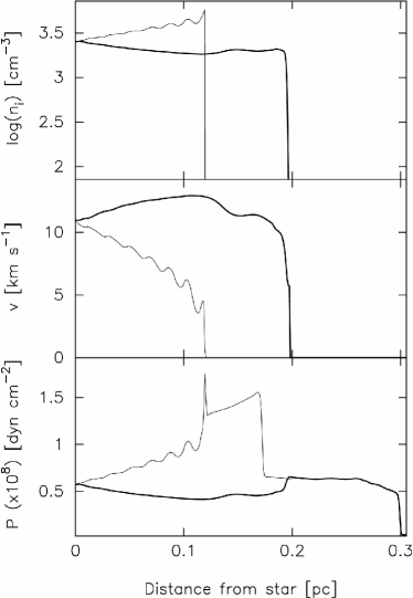
Figure 8.— Cuts along the $\mu=\pm 1$ axis of the $\alpha=2$ numerical simulation shown in Fig. 7. Top: density. Middle: velocity. Bottom: pressure. The thick solid line represents the $\mu=1$ direction and the thin solid line represents the $\mu=-1$ direction. Units are as indicated on the axes.

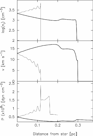
Figure 9.— Cuts along the $\mu=\pm 1$ axis of the $\alpha=3$ numerical simulation shown in Fig. 7. Top: density. Middle: velocity. Bottom: pressure. The thick solid line represents the $\mu=1$ direction and the thin solid line represents the $\mu=-1$ direction. Units are as indicated on the axes.

In Figures 7, 8 and 9 we show the results of calculations of off-center H II regions in $\alpha=2$ and $\alpha=3$ power-law density distributions. Figure 7 shows the ionized gas density, i.e. the shape of the H II regions, for both power laws after 60,000 and 50,000 yrs respectively. The density within the ionized regions is approximately constant. We note that for both models, the ionized volumes are approximately spherical, although the star is off-center. This was also noted by Mac Low et al. (2006) in their three-dimensional numerical simulations. Overplotted on Figure 7 is the shape the ionization front would have according to the approximation of Equation 15. We can see that the approximation slightly underestimates the volume of the ionized gas with respect to the numerical simulations.

In Figures 8 and 9 we show cuts along the symmetry axis, i.e. the $\mu=\pm 1$ directions, for both cases. From these figures we see that the assumption of constant density is reasonable for the $\mu=1$ (“downhill”) direction but not so good in the $\mu=-1$ direction, since the density increases with distance from the star. The pressure follows the same pattern as the density, as is to be expected in for an isothermal, $T=10^{4}$ K H II region. Outside the ionized region, in both directions, the pressure is high because the neutral shock sent out ahead of the ionization front pressurizes the gas. The velocities in the ionized gas are subsonic in the $\mu=-1$ direction and become supersonic in the $\mu=1$ direction.

The ripples in the $\mu=-1$ subsonic gas are due to the ionization front not being well resolved in this case, since the high densities lead to a very thin transition zone. The spike in the pressure is due to the heating and cooling being out of equilibrium at the unresolved ionization front. These numerical problems are not dynamically important for these simulations, since we are interested in the expansion in the $\mu=1$ direction, where the gas is supersonic and hence not affected by fluctuations in the thermal pressure. This problem was noted by Henney et al. (2005). Their solution to the problem was to reduce the effective ionization cross section, $\sigma_{0}$, by a factor of 60. In this paper, we reduce $\sigma_{0}$ by a factor of 10. Reducing the ionization cross section makes the ionization front broader and so allows it to be resolved by the numerical scheme. Since the width of the ionization front is of the order of a few photon mean free paths, where $l_{p}\propto(n\sigma_{0})^{-1}$, then the ionization front is narrower in high density gas than in low density gas, and hence more of a problem to resolve numerically in the former. In the $\mu=1$ direction, the much lower densities mean that the ionization front is easily resolved by the numerical scheme.

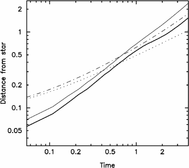
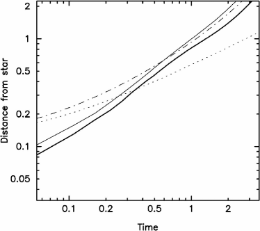
Figure 10.— Radius (in units of stellar offset radius) against time (in units of sound crossing time) in the $\mu=1$ direction, showing ionization front radius (thick solid line), shock front radius (thin solid line), analytical solution for the same parameters (dot-dashed line) and uniform density analytical solution (dashed line). Top: $\alpha=2$ numerical simulation and corresponding analytical solution. Bottom: $\alpha=3$ numerical simulation and corresponding analytical solution.

In Figure 10 a comparison of the numerical simulation and the analytic solution for the same parameters in the $\mu=1$ direction is plotted. Here, the distance scale is in units of the Strömgren radius in a medium of uniform density $n_{c}e^{-\alpha/2}$, and time is given in units of the sound crossing time of the Strömgren sphere. Since the density distribution in the $\mu=-1$ direction of the numerical simulation is different to the analytical model discussed in Section 3, we do not show a comparison graph for this case, as it is meaningless. Instead, we focus on the $\mu=1$ direction, for which the numerical simulation and analytical model density distributions are the same. We plot both the shock wave and the ionization front trajectories, together with the analytical result. For times less than about half a sound crossing time, there is not a good agreement between analytical and numerical results. This can be partly attributed to resolution effects, since the initial Strömgren radius in this high density medium is very small, and the details of the hydrodynamics are not particularly well resolved at this scale. For times greater than half a sound crossing time, the agreement between numerical and analytical solutions is very close for the remainder of the calculation. The analytical solution falls between the shock front and ionization front paths for the whole of this time.

We do not follow the numerical simulation beyond around 4 sound crossing times because part of the ionized gas volume leaves the computational grid at this point.

5. Summary

In this paper we have developed an analytical treatment for the formation and expansion of an H II region off center in a steep power-law density distribution. We find that during the initial formation stage, the H II region will remain bounded as long as the ratio of the Strömgren radius in the equivalent uniform medium at the stellar position to the stellar offset position is less than a value that depends only on the power-law exponent (see Eq. 11). In the expansion phase, the ionization front will break out (turn supersonic with respect to the ionized gas) unless pressure balance between the internal photoionized gas and the external medium is achieved before this point. For Strömgren radius to stellar offset radius ratios of more than 0.02, pressure balance is not possible for an isothermal 100 K medium in hydrostatic equilibrium and so the H II region will become unbounded, eventually, in these cases.

We performed numerical simulations to test the assumption of constant density within the ionized gas during the expansion phase adopted in § 3. We found that this assumption is valid in the “downhill” ($\theta=0$) direction from the star, but is not so good in the opposite (“uphill”, $\theta=\pi$) direction. In the $\theta=0$ direction, the numerical solution and analytical solution follow the same expansion law once the elapsed time is greater than about half a sound crossing time. We also assessed the validity of the simple analytical approximation to the ionization front shape. Although the volume of ionized gas is slightly underestimated in the analytical approximation, the effect is not significant, as evinced by the agreement between the numerical and analytic expansion laws. This gives us confidence that our simple description of the H II region expansion can provide insight into this complicated problem.

References

- Arquilla & Goldsmith (1985) Arquilla, R., & Goldsmith, P. F. 1985, ApJ, 297, 436
- Arthur & Hoare (2006) Arthur, S. J., & Hoare, M. G. 2006, ApJS, 165, 283
- Bedijn & Tenorio-Tagle (1981) Bedijn, P. J., & Tenorio-Tagle, G. 1981, A&A, 98, 85
- Bodenheimer et al. (1979) Bodenheimer, P., Tenorio-Tagle, G., & Yorke, H. W. 1979, ApJ, 233, 85
- Dyson (1977) Dyson, J. E. 1977, A&A, 59, 161
- Franco et al. (1989) Franco, J., Tenorio-Tagle, G., & Bodenheimer, P. 1989, Revista Mexicana de Astronomía y Astrofísica, vol. 18, 18, 65
- Franco et al. (1990) Franco, J., Tenorio-Tagle, G., & Bodenheimer, P. 1990, ApJ, 349, 126
- Franco et al. (2000) Franco, J., García-Barreto, J. A., & de la Fuente, E. 2000, ApJ, 544, 277
- Franco et al. (2007) Franco, J., García-Segura, G., & Kurtz, S. E. 2007, ApJ, in press (astro-ph/0508467)
- Hatchell & van der Tak (2003) Hatchell, J., & van der Tak, F. F. S. 2003, A&A, 409, 589
- Henney et al. (2005) Henney, W. J., Arthur, S. J., & García-Díaz, M. T. 2005, ApJ, 627, 813
- Lada et al. (2007) Lada, C. J., Alves, J. F., & Lombardi, M. 2007, Protostars and Planets V, eds. B. Reipurth, D. Jewitt, & K. Keil, (Tucson: University of Arizona Press), 3
- Mac Low et al. (2006) Mac Low, M.-M., Toraskar, J., Oischi, J. S. & Abel, T. 2006, ApJ, submitted (astro-ph/06055001)
- Press et al. (1992) Press, W. H., Teukolsky, S. A., Vetterling, W. T., & Flannery, B. P. 1992, Numerical Recipes in Fortran: The Art of Scientific Computing, 2nd ed., Cambridge: University Press
- Shu (1992) Shu, F. H. 1992, Physics of Astrophysics, Vol. II, University Science Books
- Shu et al. (2002) Shu, F. H., Lizano, S., Galli, D., Cantó, J., & Laughlin, G. 2002, ApJ, 580, 969
- Spitzer (1968) Spitzer, L. 1968, Diffuse Matter in Space, New York: Interscience Publication
- Tenorio-Tagle (1979) Tenorio-Tagle, G. 1979, A&A, 71, 59