Small scale aspects of flows in proximity of the turbulent/non-turbulent interface

M. Holzner¹, A. Liberzon², N. Nikitin³, W. Kinzelbach¹, A. Tsinober^2,4

¹ Institute of Environmental Engineering, ETH Zurich, CH 8093 Zurich, Switzerland
² Department of Fluid Mechanics and Heat Transfer, Faculty of Engineering, Tel Aviv University, Tel Aviv 69978, Israel
³ Institute of Mechanics, Moscow State University, 119899 Moscow, Russia
⁴ Institute for Mathematical Sciences and Department of Aeronautics, Imperial College, SW7 2AZ London, United Kingdom

 

The work reported below is a first of its kind study of the properties of turbulent flow without strong mean shear in a Newtonian fluid in proximity of the turbulent/non-turbulent interface, with emphasis on the small scale aspects. The main tools used are a three-dimensional particle tracking system (3D-PTV) allowing to measure and follow in a Lagrangian manner the field of velocity derivatives and direct numerical simulations (DNS). The comparison of flow properties in the turbulent (A), intermediate (B) and non-turbulent (C) regions in the proximity of the interface allows for direct observation of the key physical processes underlying the entrainment phenomenon. The differences between small scale strain and enstrophy are striking and point to the definite scenario of turbulent entrainment via the viscous forces originating in strain.  

Turbulent entrainment (TE) is a process of continuous transitions from laminar to turbulent flow through the boundary (hereafter referred to as interface) between the two coexisting regions of laminar and turbulent state. This process is one of the most ubiquitous phenomena in nature and technology since, in fact, most turbulent flows are partly turbulent: boundary layers, all free shear turbulent flows (jets, plumes, wakes, mixing layers), penetrative convection and mixing layers in the atmosphere and ocean, gravity currents, avalanches and clear-air turbulence.

The first physically qualitative distinction between turbulent and non-turbulent regions, made by Corrsin Corrsin43 ; Corrsin , is that turbulent regions are rotational, whereas the non-turbulent ones are (practically) potential, thus employing one of the main differences between turbulent flow and its random irrotational counterpart on the ’other’ side of the interface separating them.

The main mechanism by which non-turbulent fluid becomes turbulent as it ‘crosses’ the interface is believed to involve viscous diffusion of vorticity ($\nu\omega_{i}\nabla^{2}\omega_{i}$) at the interface Corrsin . Corrsin and Kistler Corrsin also conjectured that the stretching of vortex lines in the presence of a local gradient in vorticity at the interface leads to a steepening of this gradient since the rate of production of vorticity is proportional to the vorticity present. The mentioned processes are associated with the small scales of the flow. However, at large Reynolds numbers the entrainment rate and the propagation velocity of the interface relative to the fluid are known to be independent of viscosity (see Ref. [Tritton, ; Tsinober, ; Hunt, ] for more information and references). Therefore the slow process of diffusion into the ambient fluid must be accelerated by interaction with velocity fields of eddies of all sizes, from viscous eddies to the energy-containing eddies, so that the overall rate of entrainment is set by the large-scale parameters of the flow. This means that although the spreading is brought about by small eddies (viscosity), its rate is governed by larger eddies. The total area of the interface, over which the spreading is occurring at any instant, is determined by these larger eddies Tritton .

Until recently it was difficult to implement Corrsin’s distinction: it requires information on small scale vorticity and strain which experimentally was not accessible. This is why very little is known about the processes at small scales and in the proximity of the entrainment interface. A few exceptions are recent particle image velocimetry (PIV) and planar laser-induced fluorescence (PLIF) experiments by Westerweel et al. Westerweel ; WesterweelPRL of a jet and experiments by Holzner et al. holzner on oscillating grid turbulence, in addition to the direct numerical simulations (DNS) of a temporally developing plane wake by Bisset et al. Bisset and a similar analysis of an axisymmetric configuration by Mathew and Basu Mathew . Unfortunately, in the PIV/PLIF experiments only the azimuthal component of vorticity in a two-dimensional cross-section was accessible.

The main objective of the study presented is a systematic analysis of the small scale dynamics associated with turbulent entrainment. The special emphasis is on the processes involving the field of vorticity, $\omega_{i}$, and its production/destruction by inertial $\omega_{i}\omega_{j}s_{ij}$ and viscous $\nu\omega_{i}\nabla^{2}\omega_{i}$ processes in the proximity of the interface ($s_{ij}$ are the components of the fluctuating rate-of-strain tensor, $\nu$ is the kinematic viscosity). Studying the production of vorticity requires access to the field of strain as well (and thereby also to the dissipation, $2\nu s_{ij}s_{ij}$). We briefly recall the local budget equations for enstrophy, reading $\frac{D}{Dt}\frac{\omega^{2}}{2}=\omega_{i}\omega_{j}s_{ij}+\nu\omega_{i}\nabla^{2}\omega_{i}$ and strain, written as $\frac{D}{Dt}\frac{s^{2}}{2}=-s_{ij}s_{jk}s_{ki}-\frac{1}{4}\omega_{i}\omega_{j}s_{ij}-s_{ij}\frac{\partial^{2}p}{\partial x_{i}\partial x_{j}}+\nu s_{ij}\nabla^{2}s_{ij}$.

Experimentally, a turbulent/non-turbulent interface was realized by using the oscillating planar grid described in Holzner et al. holzner . The grid is a fine woven screen installed near the upper edge of a water filled glass tank, oscillating at a frequency of 6 Hz and an amplitude of 4 mm. The scanning method of 3D particle tracking velocimetry (3D-PTV) used here is presented in Hoyer et al. hoyer05 . In order to access the viscous term of vorticity, the postprocessing procedure was extended. Due to experimental noise it is not possible to obtain the Laplacian of vorticity, $\nu\nabla^{2}\mbox{\boldmath{$\omega$}}$, directly through differentiation as it involves second derivatives of the vorticity field. Instead, the viscous term is obtained from the local balance equation of vorticity in the form $\nabla\times\mathbf{a}=\nu\nabla^{2}\mbox{\boldmath{$\omega$}}$ by evaluating the term $\nabla\times\mathbf{a}$ from the Lagrangian tracking data. The derivatives of Lagrangian acceleration, $\partial a_{i}/\partial x_{j}$, are calculated in the same way as the derivatives of the velocity, $\partial u_{i}/\partial x_{j}$, described in Hoyer et al. hoyer05 and subsequently they are interpolated on a Eulerian grid. The number of tracked particles is about 6$\cdot$10³ in a volume of 2$\times$2$\times$1.5 cm³ and the interparticle distance is about 1 mm, which is slightly above the estimated Kolmogorov length scale, $\eta$=0.6mm. The Taylor microscale, $\lambda$, is about 7 mm. The spacing of the Eulerian grid was taken equal to the interparticle distance. Further details on the data analysis will be discussed in the forthcoming full paper. In both experiment and simulation, the Taylor microscale Reynolds number is Re_λ=50.

Direct numerical simulation (DNS) was performed in a box (side-lengths $L_{1}$, $L_{2}$, $L_{3}$) of initially still fluid. Random (in space and time) velocity perturbations are applied at the boundary $x_{2}$=0. The procedure of generating the boundary conditions is as follows. For a fixed time and in the discrete set of points, $x_{1}=k\Delta_{l}$, $x_{3}=l\Delta_{l}$ (k, l - integers), each velocity component, $u_{i}$ (i = 1, 2, 3), is calculated as $u_{i}=V_{i}\xi$, where $\xi$ is a random number within the interval $[-1,1]$ and $V_{i}$ is a given velocity amplitude. For other times and spatial points ($x_{1}$, $x_{3}$) boundary velocities are obtained by cubic interpolation in time and bilinear interpolation in space. At each time the three boundary velocity components yield zero average value over the boundary plane. The method of boundary velocity assignment determines the velocity scale, $V=\mathrm{max}(V_{i})$ and the length scale $\Delta_{l}$. Together with the viscosity of a fluid, $\nu$, these parameters define the Reynolds number $Re=V\Delta_{l}/\nu=1000$ of the simulation. The Navier-Stokes equations are solved with periodic boundary conditions for the directions $x_{1}$ and $x_{3}$, with periods $L_{1}$ and $L_{3}$, respectively. The computational domain is finite in the $x_{2}$ direction, as $x_{2}\leq L_{2}$. Shear-free conditions $\partial u_{1}/\partial x_{2}=\partial u_{3}/\partial x_{2}=u_{2}=0$ are imposed at the boundary $x_{2}$ = $L_{2}$. A mixed spectral-finite-difference method is used for the spatial discretization and the time advancement is computed by a semi-implicit Runge-Kutta method Nikitin94 . The resolution is 192$\times$192 Fourier modes in $x_{1}$ and $x_{3}$ directions and 192 grid points in $x_{2}$ direction. The local Kolmogorov length scale is twice the grid spacing.

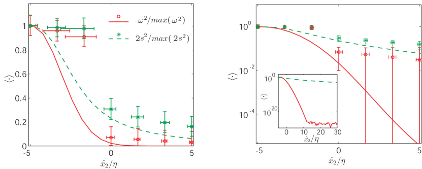
Figure 1: Average profiles of $\omega^{2}(\hat{x}_{2})$ and $2s^{2}(\hat{x}_{2})$ from PTV (symbols), and DNS (lines) relative to the interface, $\hat{x}_{2}=x_{2}-x_{2}^{*}$, on linear scale (left) and on log-scale (right). The values are normalized by the respective maxima ($\mathrm{max}$($\omega^{2}$)$\approx\mathrm{max}$(2s${}^{2})\approx$3.6 s^-2 for PTV and 3.0 for DNS). The horizontal error bars display the sensitivity of the experimental result on the enstrophy threshold, 0.5-2.5 $s^{-2}$, the vertical error bars represent the accuracy of the measurement. The symbol $\langle\cdot\rangle$ denotes the ensemble average of the respective quantity

In both experiment and simulation, turbulence is generated at the plane $x_{2}$ =0 and propagates along $x_{2}>0$. Firstly, the interface is identified at $x_{2}^{*}(t)$, using a fixed threshold of enstrophy, (for details see Ref. [holzner, ] and references therein) and the analysis is done with respect to the interface location, as in Fig. 1, in which profiles of enstrophy, $\omega^{2}=\omega_{i}\omega_{i}$ and strain rate, $s^{2}=s_{ij}s_{ij}$, averaged over homogeneous $x_{1},x_{3}$ directions on linear scale (left) and log scale (right), are shown. The distance to the interface, $\hat{x}_{2}$ is normalized by the Kolmogorov length scale, $\eta$. The ’proximity’ or ’region of the interface’ hereafter refers to the interval -5$<\hat{x}_{2}/\eta<$5. We observe that the rate of strain on the non-turbulent side of the interface remains high in contrast to enstrophy which drops much more steeply. Experimentally it is not possible to obtain enstrophy lower than a small (but finite) level of noise. This is one of the reasons why comparison to DNS is presented for all the results. In the DNS, the numerical noise level is reached at $\hat{x_{2}}/\eta>$10 and this level is about 25 decades lower in magnitude, see the inset in Fig. 1 (right).

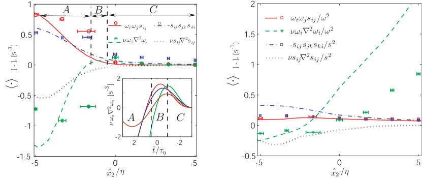
Figure 2: Average profiles of production and viscous destruction terms of strain and enstrophy (left) and their rates (right). The inset shows the individual Lagrangian trajectories of $\nu\omega_{i}\nabla^{2}\omega_{i}\$ obtained from PTV. Lines are from DNS, symbols are from PTV

Fig. 2 shows profiles of production and viscous terms of strain and enstrophy (left) and their rates (right). We note that the viscous term, $\nu\omega_{i}\nabla^{2}\omega_{i}$, exhibits a remarkable behavior showing a distinct maximum in the region of the interface. In addition, the individual Lagrangian trajectories (examples are shown in the inset in Fig. 2, where the abscissa is $\hat{t}=t-t^{\ast}$, normalized by the Kolmogorov time scale, $\tau_{\eta}$, and $t^{\ast}$ is analogous to $x_{2}^{\ast}$) possess such an extremum. Therefore, we use the maximum of the viscous term as the exact location of the interface, defined in a physically more appealing way than the threshold-dependent crossing of $\hat{x}_{2}/\eta$=0. For the further analysis we define three physically distinct regions of the interface with respect to the maximum of $\nu\omega_{i}\nabla^{2}\omega_{i}$ (marked in Fig. 2): (A) the turbulent region, in which the behavior of the viscous term is ‘normal’, i.e. it is negative in the mean, (B) the interval between the peak and the point where $\langle$$\nu\omega_{i}\nabla^{2}\omega_{i}$$\rangle$=0 is termed intermediate region (with the ’abnormal’ viscous production) and, (C) the non-turbulent region from the peak to $\hat{x}_{2}/\eta$=5. The positiveness of both $\omega_{i}\omega_{j}s_{ij}$ and $\nu\omega_{i}\nabla^{2}\omega_{i}$ is a peculiar feature of the regions B and C, in contrast to region A, where, in the mean, $\nu\omega_{i}\nabla^{2}\omega_{i}$ contributes to the destruction and $\omega_{i}\omega_{j}s_{ij}$ to the production of $\omega^{2}$. It is noteworthy that strain behaves rather differently from vorticity. In particular, the viscous term, $\nu s_{ij}\nabla^{2}s_{ij}$, is negative in the mean in all three regions, i.e. it is not building up $s^{2}$. In Fig. 2 we see also that strain production, -$s_{ij}s_{jk}s_{ki}$, is significant and it is (in the mean) not balanced by $\nu s_{ij}\nabla^{2}s_{ij}$ in region C. When the rates of quantities are considered it appears (Fig. 2, right) that the role of viscous production is even more important: the term $\nu\omega_{i}\nabla^{2}\omega_{i}$/$\omega^{2}$ attains high positive values in region C, decreases along region B and finally becomes negative in region A (balancing the average $\omega_{i}\omega_{j}s_{ij}$/$\omega^{2}$). In contrast, the term $\omega_{i}\omega_{j}s_{ij}$/$\omega^{2}$ and the analogous rates of the strain viscous and production terms do not change as drastically and remain of the same sign.

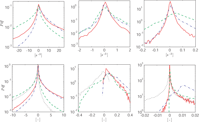
Figure 3: PDF of various quantities from experiment (top) and simulation (bottom) according to the division in 3 regions: turbulent (left), intermediate (center) and non-turbulent (right). $\omega_{i}\omega_{j}s_{ij}\$ (–), $\nu\omega_{i}\nabla^{2}\omega_{i}$ (- -), -$s_{ij}s_{jk}s_{ki}\$ (- $\cdot$), $\nu s_{ij}\nabla^{2}s_{ij}$ ($\cdots$, only bottom)

Fig. 3 presents the estimations of probability density functions (PDFs) of the relevant terms from the different regions (A,B, and C, from left to right; PTV top, DNS bottom). Consistently with the other results, the PDFs of both $\omega_{i}\omega_{j}s_{ij}$ and $\nu\omega_{i}\nabla^{2}\omega_{i}$ are positively skewed in regions B and C. In region B we note that the probability of negative events of $\nu\omega_{i}\nabla^{2}\omega_{i}$ and positive events of $\omega_{i}\omega_{j}s_{ij}$ increases as compared to region C. Finally, as expected, in region A the PDF of $\nu\omega_{i}\nabla^{2}\omega_{i}$ is negatively skewed. The changes of the strain production and viscous terms between the regions A-C are less drastic. Essentially, -$s_{ij}s_{jk}s_{ki}$ is positively and $\nu s_{ij}\nabla^{2}s_{ij}$ is negatively skewed in all the three regions.

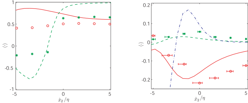
Figure 4: (left) Cosines of the angle between vorticity and W (–,o) and between vorticity and $\nu\nabla^{2}\mbox{\boldmath{$\omega$}}$ (- -,$\ast$). (right) Invariants, $Q$ (–, o), $R$ (- -,$\ast$), $S$ ($-\cdot-$, only DNS). Lines are from DNS, symbols are from PTV

For the understanding of the interaction of strain and enstrophy in the proximity of the interface it is very instructive to look at the invariants of the gradient tensor: $Q=\omega^{2}-2s^{2}=-\nabla^{2}P$ shows the relative strength of vorticity and strain, $R$=-1/3($s_{ij}s_{jk}s_{ki}\$+3/4$\omega_{i}\omega_{j}s_{ij}\$) relates to their production terms, and $S$ is the quantity related to the two viscous terms, $S=\nu\omega_{i}\nabla^{2}\omega_{i}\ -2\nu s_{ij}\nabla^{2}s_{ij}\$ (Fig. 4, right). Since the mean values of $Q,R$ and $S$ vanish identically for homogeneous turbulence, their nonzero values indicate the degree of inhomogeneity in the proximity of the interface. Apparently, inhomogeneity is the property which is maximal where also $\nu\omega_{i}\nabla^{2}\omega_{i}$ is maximal. In the same context it is also interesting to look at the cosine of the angle between vorticity and its Laplacian, $\nabla^{2}\omega_{i}$, shown in Fig. 4 (left), which exhibits significant changes across the regions A,B, and C. The observed transition from positive (alignment) to negative (anti-alignment) values is in agreement with the qualitatively different behavior of $\nu\omega_{i}\nabla^{2}\omega_{i}$ in these regions. In contrast to that, the alignment between vorticity and the vortex stretching vector, $W_{i}=\omega_{j}s_{ij}$, changes only weakly throughout regions A-C and is consistent with the positiveness of $\langle$$\omega_{i}\omega_{j}s_{ij}$$\rangle$ mentioned above. The results indicate that an interpretation of the viscous term $\nu\omega_{i}\nabla^{2}\omega_{i}$ as interaction between strain and vorticity due to viscosity (i.e. due to the curl of the viscous force originating from the divergence of the strain tensor) is physically more appealing than ’simple’ diffusion of vorticity due to viscosity. We emphasize that $\nu\omega_{i}\nabla^{2}\omega_{i}$ is the interaction of vorticity and strain since (e.g., Ref. [Batchelor, ]) $\nu\nabla^{2}\mbox{\boldmath{$\omega$}}$$=1/\rho\ \nabla\times\mathbf{F}^{s}$, where $\ F_{i}^{s}=2\nu\partial/\partial x_{k}\{s_{ik}\}$ and $\rho$ is the fluid density.

In summary, we analyzed small scale enstrophy and strain dynamics in proximity of a turbulent/non-turbulent interface without strong mean shear. The experimental results are in good agreement with the simulation, at least on a qualitative level, which is considered as a clear indication for the reliability of both methods. The behavior of vorticity-related quantities is very different from the strain-related counterparts. For example, the viscous term is not responsible for building up strain as strain is destroyed by $\nu s_{ij}\nabla^{2}s_{ij}$ in all three regions. In addition, the analysis of these quantities with respect to the distance from the interface reveals the range of influence of $\nu\omega_{i}\nabla^{2}\omega_{i}\$ and $\nu s_{ij}\nabla^{2}s_{ij}\$ into the non-turbulent region. We also found that both $\omega_{i}\omega_{j}s_{ij}$ and $\nu\omega_{i}\nabla^{2}\omega_{i}$ are responsible for the increase of $\omega^{2}$ at the interface and substantiate the physical interpretation of the term $\nu\omega_{i}\nabla^{2}\omega_{i}$ as viscous interaction, in analogy to $\omega_{i}\omega_{j}s_{ij}$, commonly referred to as the inviscid interaction of vorticity and strain.

We gratefully acknowledge the support of this work by ETH Grant No. 0-20151-03. The work of N. Nikitin was supported by the Russian Foundation for Basic Research under the grant 05-01-00607.

References

-
(1)
Corrsin S. (1943) Investigation of flow in an axially symmetric
heated jet in air. NACA ACR 3L23 and Wartime Rept W94
1946.
http://ntrs.nasa.gov/search.jsp?R=614125&id=4&qs=N%3D4294804713 -
(2)
Corrsin S. and Kistler A.L. (1954, 1955) The
free-stream boundaries of turbulent flows. NACA, TN-3133,
TR-1244, 1033-1064.
http://ntrs.nasa.gov/search.jsp?R=84354&id=9&qs=N%3D4294804713 - (3) Tritton, D. J. (1988) Physical fluid dynamics. 2nd ed., Clarendon Press, Oxford, UK.
- (4) Tsinober A. (2001) An informal introduction to turbulence. Springer, Berlin, New York.
- (5) Hunt J.C.R., Eames I., Westerweel J. (2006) Mechanics of inhomogeneous turbulence and interfacial layers. J. Fluid Mech., 554, 449-519.
- (6) Westerweel J., Hoffmann T., Fukushima C. and Hunt J.C.R. (2002) The turbulent/non-turbulent interface at the outer boundary of a self-similar turbulent jet. Exp. Fluids 33, 873-878.
- (7) Westerweel J., Fukushima C., Pedersen J.M. & Hunt J. (2005) Mechanics of the turbulent/non-turbulent interface of a jet. Phys. Rev. Lett. 95, 174501.
- (8) Holzner M., Liberzon A., Guala M., Tsinober A., Kinzelbach W. (2006) An experimental study on the propagation of a turbulent front generated by an oscillating grid. Exp. Fluids. 41(5), 711-719.
- (9) Bisset D.K., Hunt J.C.R. and Rogers M.M. (2002) The turbulent/non-turbulent interface bounding a far wake. J. Fluid Mech. 451, 383-410.
- (10) Mathew J., Basu A.J. (2002) Some characteristics of entrainment at a cylindrical turbulence boundary. Phys. Fluids, 14(7), 2065-2072.
- (11) Hoyer K., Holzner M., Lüthi B., Guala M., Liberzon A. and Kinzelbach W. (2005) 3D scanning particle tracking velocimetry. Exp. Fluids 39(5), 923 - 934.
- (12) Nikitin N. (1994) A spectral finite-difference method of calculating turbulent flows of an incompressible fluid in pipes and channels. Comp. Maths Math. Phys., 34(6), 785–798 and Nikitin N. (1996) Statistical characteristics of wall turbulence. Fluid Dynamics, 31, 361-370.
- (13) Batchelor G.K. (2000) An Introduction to Fluid Dynamics. Cambridge University Press, London, UK.