Updating the Phase Diagram of the Gross-Neveu Model in $2+1$ Dimensions

Abstract

The method of optimized perturbation theory (OPT) is used to study the phase diagram of the massless Gross-Neveu model in $2+1$ dimensions. In the temperature and chemical potential plane, our results give strong support to the existence of a tricritical point and line of first order phase transition, previously only suspected to exist from extensive lattice Monte Carlo simulations. In addition of presenting these results we discuss how the OPT can be implemented in conjunction with the Landau expansion in order to determine all the relevant critical quantities.

keywords: chiral phase transition, Gross-Neveu model, four-Fermi models, nonperturbative thermodynamics

I Introduction

The use of exactly solvable models and methods leading to analytical solutions has always been important in physics in general. Models of particular interest are those that display some physical correspondence to the physics of quantum chromodynamics (QCD) or that may give insights to the difficult task, given its nonperturbative nature, of analyzing the phase structure at finite temperatures and densities. This is also the kind of situation, regarding phase transitions in a hot and dense medium, that is expected to be realized in the early universe and in the recent experiments involving heavy-ion collisions. The use of appropriate techniques and models in the context of quantum field theory that can increase our knowledge on this kind of phenomena are then timely and important. One such phenomenon of topical interest is the study of the chiral symmetry restoration (CSR) in QCD. However, due to the intrinsic difficulty of approaching directly this study in the context of QCD itself, other more tractable models have been extensively used. Among them, the simplest fermionic model displaying many properties common to QCD is the Gross-Neveu (GN) model GN . For instance, in 2+1 dimensions it can exhibit a discrete spontaneous chiral symmetry breaking (CSB) that happens for a critical coupling at zero temperature and density, while its spectrum can contain excitations like baryons as well as mesons (which are composite fermionic states). Even though it is a quartic interacting fermion model, thus nonrenormalizable (in 2+1 dimensions) in ordinary perturbation theory, it is renormalizable in a $1/N$ expansion (where $N$ denotes the number of fermion species) and it is exactly soluble in the large-$N$ limit Park . These properties make this effective model one of the simplest and most useful frameworks for understanding some of the important physical features displayed by QCD.

For the reasons above, the GN model is a perfect laboratory for studying symmetry aspects in a hot and dense medium and outside the QCD realm, the model by its own and its extensions may also have applications in condensed matter physics in the understanding of the properties of fermion liquids and high-$T_{c}$ superconductivity models condmatter . Besides being studied analytically mostly with the large-$N$ expansion technique, there are a large number of works studying the GN model numerically from the lattice Monte-Carlo perspective lattice1 ; lattice2 (for an introduction to lattice QCD, its problems in implementation and applications to effective models, like the GN one, see latticeQCD and references therein). Among the interesting thermodynamical properties of the GN model demonstrated by the large-$N$ technique is the existence of a line of second order CSR in the temperature and chemical potential ($T,\mu$) plane, starting at a value ($T_{c},0$) and ending, abruptly, at a first order transition point ($0,\mu_{c}$) Park ; klimenko . While this phase structure was verified by lattice simulations with finite number of fermion species, $N$, in Ref. lattice2 some indication was given for the existence of a first order transition line starting at a tricritical point ($T_{\rm tcr},\mu_{\rm tcr}$) and ending at $\sim(0,\mu_{c})$. However, the precise position of this tricritical point in the phase diagram could not be determined. Even within the $1/N$ expansion, there are no results available on the phase structure of the 2+1 dimensional GN model beyond the leading order, due to the appearance of complicate integrals (note however that there are results up to ${\cal O}(1/N^{2})$ for the critical exponents Gracey of the bulk transition). It then becomes an important and interesting issue to investigate whether there is indeed a tricritical point for the GN model at finite $N$ in 2+1 dimensions and by which method we would be able to localize it in a robust form. By doing so, we expect to have a much better understanding of the chiral symmetry restoration problem at finite $T$ and $\mu$ not only in this model but also to have eventually a better knowledge of a similar behavior that may happen in QCD or even in analog condensed matter systems. In this work we study the 2+1 dimensional GN model beyond the large-$N$ limit and, to obtain its phase diagram at finite $T$ and $\mu$, we make use of the method of the optimized perturbation theory (OPT) (also known as linear $\delta$ expansion) LDE . Here, we discuss how this method can be used to extract useful information, regarding critical quantities, from the Landau expansion of the free energy density.

This paper is organized as follows. In the next section we introduce the model, presenting the OPT free energy density. In Sec. III, we discuss optimization issues related to the Landau expansion of the free energy density. Our results for the $(T,\mu)$ phase diagram as well as for the critical quantities are presented in Sec. IV, showing the existence of tricritical point for finite values of $N$. Our conclusions and perspectives for future applications are discussed in Sec. V.

II The Interpolated Gross-Neveu Model

The GN model is described by a Lagrangian density for a $N$ component fermion field $\psi_{j}$ ($j=1,\ldots,N$) with local quartic fermion interaction which is defined by GN (in this work all our expressions are defined in Euclidean space)

$${\cal L}=\bar{\psi}_{j}\not\!\partial\psi_{j}-\frac{\lambda}{2N}({\bar{\psi}_{j}}\psi_{j})^{2}\;,$$ (1)

where, in 2+1 dimensions, the fermion fields are treated as four-component Dirac spinors and the $\gamma_{\mu}$ matrices are defined in the $4\times 4$ representation. In this way, Eq. (1) is invariant under the discrete chiral transformations $\psi_{j}\to\gamma_{5}\psi_{j}$ and $\bar{\psi}_{j}\to-\bar{\psi}_{j}\gamma_{5}$. Though it also has a continuous flavor symmetry we will only be interested in the case of discrete symmetry, recalling a general no-go theorem in 2+1 dimensions that forbids spontaneous symmetry breaking of a continuous symmetry at any finite temperature coleman .

The implementation of the OPT within this model is reviewed in a previous application LPR to the 1+1 dimensional case. In practice, one considers the original theory, Eq. (1), adding a quadratic (in the fermion field) term $(1-\delta)\eta{\bar{\psi}_{j}}\psi_{j}$ where $\eta$ is an arbitrary mass parameter and $\delta$ is a bookkeeping parameter which labels the order at which the OPT is being performed. At the same time, $\lambda\to\delta\lambda$. Also, as conventional, we rewrite the quartic term by introducing an auxiliary scalar field $\sigma$. Then, Eq. (1) acquires its OPT form LPR

$${\cal L}_{\delta}=\bar{\psi}_{j}\not\!\partial\psi_{j}+\delta\sigma{\bar{\psi}_{j}}\psi_{j}+(1-\delta)\eta{\bar{\psi}_{j}}\psi_{j}+\frac{\delta N}{2\lambda}\sigma^{2}\;.$$ (2)

The OPT then describes an interpolated theory with a fermion propagator $[\not\!P+(1-\delta)\eta+\delta\sigma_{c}]^{-1}$, Yukawa vertex $\delta$ and $\sigma$ propagator $\lambda/(N\delta)$. Any quantity $\Phi^{(k)}$ is then evaluated to an order-$\delta^{k}$ using these new Feynman rules. As shown in the many previous applications using this method moreOPT , it operates for any $N$ and is free from infrared divergences. Nonperturbative results for the original ($\eta$-independent) theory are obtained by optimizing $\Phi^{(k)}$ with respect to $\eta$ at $\delta=1$. One standard and largely adopted optimization procedure is the variational criterion known as the Principle of Minimal Sensitivity (PMS) which fixes $\eta$ by requiring, order by order, that $d\Phi^{(k)}/d\eta=0$ PMS .

From Eq. (2), we are interested in evaluating the effective potential for the auxiliary scalar background field, $V_{\rm eff}(\sigma_{c})$, obtained once all fermion fields and fluctuations around the scalar background field are integrated out Park . From this quantity all the thermodynamics for the model can be derived. In particular, CSB is signaled by a non-vanishing vacuum expectation value for $\sigma$, ${\bar{\sigma}}_{c}\equiv\langle\sigma\rangle$, which is a minimum of $V_{\rm eff}(\sigma_{c})$.

Figure 1: Feynman diagrams contributing to $V_{\rm eff}$ to ${\cal O}(\delta^{1})$. The continuous lines are (the $\delta$ independent) fermion propagators, the black dot is an insertion of $\delta(\sigma_{c}-\eta)$, while the dashed line represents the $\sigma$ propagator.

In Fig. 1 we show all the Feynman diagrams contributing to $V_{\rm eff}(\sigma_{c})$ up to ${\cal O}(\delta)$. Note that already at this first order in the OPT a correction that goes beyond the large-$N$ expansion is included. The first two diagrams in Fig. 1 are ${\cal O}(1/N^{0})$, while the third one contains an exchange type of self-energy as insertion and brings the first ${\cal O}(1/N)$ correction to $V_{\rm eff}(\sigma_{c})$. Explicitly, we have for all the terms shown in Fig. 1 the expression

$$\frac{V_{\rm eff,\delta^{1}}(\sigma_{c},\eta)}{N}=\delta\frac{\sigma_{c}^{2}}{2\lambda}-\int_{p}^{(T)}{\rm tr}\,\ln(\not\!P+\eta)-\delta(\sigma_{c}-\eta)\int_{p}^{(T)}{\rm tr}\frac{1}{\not\!P+\eta}+\delta\frac{\lambda}{2N}\int_{p}^{(T)}\int_{q}^{(T)}{\rm tr}\,\frac{1}{(\not\!P+\eta)(\not\!Q+\eta)}\;,$$ (3)

where the Euclidean momenta are given by $P=(P_{0},{\bf p})$ and $P_{0}=(2n+1)\pi T-i\mu$, with $n=0,\pm 1,\pm 2,\ldots$. In the above equation we have used the compact notation:

$$\int_{p}^{(T)}=T\sum_{n=-\infty}^{+\infty}\int\frac{d^{d-1}p}{(2\pi)^{d-1}},$$

with all momentum space integrals done with dimensional regularization, $d=3-\epsilon$, while renormalization can be implemented in the modified minimal subtraction scheme ($\overline{\rm MS}$). All the contributions considered in Eq. (3) are actually finite in dimensional regularization. In Ref. long we have considered the free energy up to order-$\delta^{2}$, at $T=0$ and $\mu=0$, where the first divergences show up and we refer the interested reader to that work for a detailed account on the renormalization problem of the 2+1 dimensional GN model in the OPT. Let us only emphasize here that though the model is not perturbatively renormalizable, to ${\cal O}(\delta^{2})$ and within dimensional regularization, we only need standard (i.e. mass, wave-function, etc) renormalization counterterms to render the effective potential calculation finite long .

III Landau’s Expansion and the Optimization Procedure

The effective potential, $V_{\rm eff}(\sigma_{c})$, is a natural quantity to be optimized in the spirit of the PMS procedure since it represents the system’s (Landau) free energy density, whose knowledge allows for a complete analysis of all relevant thermodynamical properties. Also, as explained in Ref. LPR , by optimizing the free energy we can guarantee that not only the exact large-$N$ results are already obtained at leading order in the OPT, but also at any subsequent order, provided that one stays within the $N\to\infty$ limit (at first order in the OPT this corresponds to dropping the third diagram in Fig. 1 and applying the optimization procedure to the first two diagrams). This shows that the OPT is convergent at any order in the OPT when contrasted with the large-$N$ predictions. This result is valid for any temperature or value of chemical potential and applies as well to any number of dimensions (for other accounts on the convergence of the OPT in the context of quantum field theory, please see conv and references therein). Let us consider the expression for $V_{\rm eff}(\sigma_{c})$ at ${\cal O}(\delta)$ with $\lambda\to-\lambda$ in which case chiral symmetry is broken at $T=0=\mu$. After taking the traces in Eq. (3), rearranging the terms and employing the redefinition of the coupling, $\Lambda=\pi/|\lambda|$, one obtains

$$\frac{V_{{\rm eff},\delta^{1}}}{N}=-\delta\frac{\sigma_{c}^{2}\Lambda}{2\pi}-2{\cal I}_{0}(\eta,\mu,T)+4\delta\,\eta\,(\eta-\sigma_{c})\,{\cal I}_{1}(\eta,\mu,T)-\delta\frac{2\pi}{N\Lambda}\eta^{2}[{\cal I}_{1}(\eta,\mu,T)]^{2}-\delta\frac{2\pi}{N\Lambda}[{\cal I}_{2}(\eta,\mu,T)]^{2}\,\,,$$ (4)

where

$${\cal I}_{0}(\eta,\mu,T)=\int_{p}^{(T)}\ln\left(P^{2}+\eta^{2}\right)\,\,,\,\,{\cal I}_{1}(\eta,\mu,T)=\int_{p}^{(T)}\frac{1}{P^{2}+\eta^{2}}\,\,\,,\,\,\,{\cal I}_{2}(\eta,\mu,T)=\int_{p}^{(T)}\frac{P_{0}}{P^{2}+\eta^{2}}\;.$$ (5)

Setting $\delta=1$ and applying the PMS to Eq. (4) we obtain a self-consistent equation for the optimized mass

$${\bar{\eta}}=\sigma_{c}+\frac{\pi}{N\Lambda}\left\{\eta{\cal I}_{1}(\eta,\mu,T)+{\cal I}_{2}(\eta,\mu,T){\cal I}_{2}^{\prime}(\eta,\mu,T)\left[{\cal I}_{1}(\eta,\mu,T)+\eta{\cal I}_{1}^{\prime}(\eta,\mu,T)\right]^{-1}\right\}\Bigr{|}_{\eta={\bar{\eta}}}\,\,,$$ (6)

where the primes indicate derivatives with respect to $\eta$. It can easily be verified that one immediate consequence of Eq. (6) is that for $N\to\infty$ we have ${\bar{\eta}}=\sigma_{c}$, thus retrieving all large-$N$ results, as mentioned in the previous paragraph. All the details concerning the Matsubara sums and dimensional regularized integrals can be found in Ref. long . (Note that the sum over the Matsubara frequencies and all space momentum integrals can be evaluated analytically at this first $\delta$ order here considered).

In the case $\mu=0$, Eq. (6) factorizes in a nice way which allows us to understand how the OPT resums the series producing non-perturbative results. Using ${\cal I}_{2}(\eta,0,T)=0$ (see Ref. long ) we can write Eq. (6) in the self-consistent form:

$${\bar{\eta}}=\sigma_{c}+\frac{\pi}{N\Lambda}\bar{\eta}\>{\cal I}_{1}(\bar{\eta},0,T)\,\,.$$ (7)

Explicitly, ${\cal I}_{1}(\bar{\eta},\mu,T)$ is given by (from the Matsubara sum and momentum integration)

$${\cal I}_{1}(\bar{\eta},\mu,T)=-\frac{T}{4\pi}\left\{\frac{|\bar{\eta}|}{T}+\ln\left[1+e^{-(|\bar{\eta}|-|\mu|)/T}\right]+\ln\left[1+e^{-(|{\bar{\eta}}|+|\mu|)/T}\right]\right\}\;.$$ (8)

The resummation becomes even easier to be visualized if one notes that $\Sigma_{\rm exc}(\bar{\eta},0,T)=\pi\bar{\eta}/(N\Lambda)\>{\cal I}_{1}(\bar{\eta},0,T)$, where $\Sigma_{\rm exc}(\bar{\eta},0,T)$ represents an exchange (rainbow, Fock) type of contribution so that, at $\mu=0$, one may write ${\bar{\eta}}=\sigma_{c}+\Sigma_{\rm exc}(\bar{\eta},0,T)$. Note that prior to optimization, the terms contributing to $V_{\rm eff}$ to first order are the ones given by Eq. (3), represented by the diagrams shown in Fig. 1. Upon optimization the diagrams are dressed by rainbow type of self-energy contributions that originates from the first nontrivial diagram represented by the third term in Fig. 1. This was expected since at order-$\delta$ the perturbative OPT effective potential receives information about this type of topology only. The OPT will then gather all powers of $1/N$ corresponding to the (rainbow) class of diagram. In other words, the simple evaluation of a first topologically distinct diagram is already able to bring non-perturbative information concerning that type of contribution. If one proceeds to order-$\delta^{2}$, information about corrections to the scalar propagator as well as Yukawa vertex will enter the perturbative effective potential. Then, the PMS will dress up these perturbative contributions and so on. Of course this rather simple OPT/PMS procedure does not give all the truly non-perturbative and higher order contributions, such as the genuine $1/N^{2}$ and higher order corrections, but is just one particular class of graphs that are being resummed in this way. It nevertheless gives a non trivial result that goes beyond the standard $1/N$ order.

Let us now consider the $T=\mu=0$ case. By optimizing $V_{\rm eff}(\sigma_{c})$, at ${\cal O}(\delta)$, it is very easy to show that one finds the optimum value ${\bar{\eta}}={\bar{\sigma}}_{c}{\cal F}(N)$, where ${\bar{\sigma}}_{c}$ is the minimum of $V_{\rm eff}(\sigma_{c})$, and ${\cal F}(N)=1-1/(4N)$ is a characteristic function that will appear in all our expressions. At this value of $\eta$ and computing the extremum for the effective potential for $\sigma_{c}$, we obtain that the order parameter is given by

$${\bar{\sigma}}_{c}=\Lambda{\cal F}(N)^{-2}\;.$$ (9)

Note that the scalar field vacuum expectation value ${\bar{\sigma}}_{c}$ sets the natural scale for CSB. We could express all our other results in terms of ${\bar{\sigma}}_{c}$, but here we find more convenient to normalize all critical quantities in terms of just $\Lambda$ (after all this is just a scaling choice). In Ref. long the result for the critical temperature has been obtained in a similar and completely analytic fashion producing the OPT result

$$T_{c}(\mu=0)=\Lambda/\left[2\ln 2\,{\cal F}(N)\right]\;.$$ (10)

However, an interesting alternative is to obtain $T_{c}$ using the Landau expansion for the free energy density, which is valid for small values of the order parameter. The Landau’s expansion (for small $\sigma_{c}$) for $V_{\rm eff}$ can be expressed in the general form

$$V_{\rm eff}(\sigma_{c},\mu,T)\simeq V_{0}+\frac{1}{2}a(\mu,T)\>\sigma_{c}^{2}+\frac{1}{4}b(\mu,T)\>\sigma_{c}^{4}+\frac{1}{6}c(\mu,T)\>\sigma_{c}^{6}\;,$$ (11)

where $V_{0}$ is a constant (field independent) energy term. Note that only even powers of $\sigma_{c}$ are allowed due to the original chiral symmetry of the model. The coefficients $a,b$ and $c$ appearing in Eq. (11) can be obtained, respectively, by a second, fourth and sixth derivative of the free energy density expansion at $\sigma_{c}=0$. Higher order terms in the expansion (11) can be verified to be much smaller than the first order terms and can be consistently neglected.

Lets recall that the expression of the free energy in the form (11) is the simplest one able to exhibit a rich phase structure, allowing also for studying tricritical phenomena. In particular note that a tricritical point can emerge whenever we have three phases coexisting simultaneously. For the above potential, Eq. (11), one can have a second order phase transition when the coefficient of the quadratic term vanishes ($a=0$) and $b>0,c>0$. A first order transition happens for the case of $b<0,c>0$. The tricritical point occurs when both the quadratic and quartic coefficients vanish, $a=b=0$ (with $c>0$). Thus, Eq. (11) offers a simple and immediate way for analyzing the phase structure of our model. For instance, to obtain $T_{c}$ at $\mu=0$ one only needs to consider Eq. (11) to order-$\sigma_{c}^{4}$ with $b>0$ to assure that the potential is bounded from below. Then, the solution of $a(0,T_{c})=0$ sets the critical temperature. However, in order to use Landau’s expansion we must have $V_{\rm eff}$ in terms of $\sigma_{c}$, $\mu$ and $T$ only (apart from $N$ and the scale $\Lambda$, of course). In principle, this can be done by using the PMS relation, Eq. (6). As one can easily check the large $N$ result, $T_{c}=\Lambda/(2\ln 2)$ is quickly recovered by solving $a(0,T_{c})=0$ with the latter obtained from Eq. (4) with ${\bar{\eta}}=\sigma_{c}$. Now, at finite $N$, $\bar{\eta}$ depends on $\sigma_{c}$ in a highly nonlinear way and the use of Landau’s method in conjunction with the OPT-PMS does not appear to be straightforward. However, Eq. (7) can then be easily solved numerically by iteration. Let us consider the first order (in the iteration) approximate PMS solution (PMS1)

$${\bar{\eta}^{(1)}}\simeq\sigma_{c}+\frac{\pi}{N\Lambda}{\bar{\eta}}\>{\cal I}_{1}({\bar{\eta}},0,T)\Bigr{|}_{{\bar{\eta}}=\sigma_{c}}\,\,,$$ (12)

and to access the convergence of the solutions, let us also consider the next approximation (PMS2) by doing ${\bar{\eta}}\to{\bar{\eta}}^{(1)}$ on the right hand side of Eq. (7). In Table I we compare the results given by PMS1 and PMS2 with the analytical relation $T_{c}=\Lambda/[2\ln 2\,{\cal F}(N)]$, Eq. (10), for $\mu=0$.

$N$	$T_{c},Eq.(\ref{Tc})$	$T_{c}^{\rm PMS1}$	$T_{c}^{\rm PMS2}$
1	0.961797	0.979106	0.963579
3	0.786925	0.786983	0.786925
4	0.769438	0.769454	0.769437
6	0.752710	0.752713	0.752710
10	0.739844	0.739844	0.739844

Table 1: The critical temperature, $T_{c}$ (at $\mu=0$ and in units of $\Lambda$), obtained with the OPT in three alternative ways for different values of $N$. We have considered as much digits as we needed to establish eventual numerical differences.

This shows that even the PMS1 approximation gives excellent results supporting the possibility of applying the OPT-PMS in conjunction with Landau’s expansion. Especially, we notice that the results quickly converge for $N>4$ but even for the extreme case $N=1$ the agreement is rather good (higher than $99\%$).

The reader should carefully note that we have written our results, in Table I, up to seven digits just to compare the two numerical iterative optimization procedures, PMS1 and PMS2 with the analytical solution, Eq. (10). We have considered as much digits as were needed in order to establish the eventual numerical differences. By no means this otherwise excessive number of digits is intended to reflect the intrinsic accuracy of the OPT method at lowest order. At the end of the next section we briefly comment on the accuracy of the OPT based on the results at next order ${\cal O}(\delta^{2})$.

IV The Phase Diagram in the OPT

Let us now present the phase diagram for the three dimensional model. Since the results for the cases $T=\mu=0$ and $T\neq 0,\mu=0$ have been discussed in the previous section let us discuss the case $T=0$ and $\mu\neq 0$ for which the relation ${\bar{\eta}}={\bar{\sigma}}_{c}\,{\cal F}(N)$ is still valid (the reader is referred to Ref. long for details concerning the evaluation of integrals and Matsubara’s sums). In this case, CSR is found to happen at a critical value for the chemical potential, $\mu_{c}$, which is obtained as follows. We first note that for $\mu=0$ (and $T=0$, as shown previously) the effective potential has a minimum at the value of $\bar{\sigma}_{c}=\Lambda{\cal F}(N)^{-2}$, as evaluated above. For $\mu\neq 0$ the effective potential acquires another minimum that gets degenerate with the first at a value of chemical potential $\mu_{c}$, where $\bar{\sigma}_{c}=0$. At this point we then find that $V_{\rm eff}(\bar{\sigma}_{c}=0,\mu=\mu_{c},T=0)\equiv V_{\rm eff}(\bar{\sigma}_{c},\mu=0,T=0)$, from where we get, after some algebra, that the critical value for the chemical potential satisfies the equation

$$|\mu_{c}|=\frac{\Lambda}{{\cal F}(N)}\,\left(1+\frac{3}{16N}\>\frac{|\mu_{c}|}{\Lambda}\right)^{-1/3}\;.$$ (13)

Eq. (13) is a forth order equation for $\mu_{c}/\Lambda$, which is much simpler to solve by iteration, converging very quickly since $\mu/\Lambda$ is ${\cal O}(1)$. For example, at $N=3$, one finds $\mu_{c}\simeq 1.067\Lambda$, which agrees with a full numerical evaluation of the complete $T$ and $\mu$ dependent expression (3) at ${\cal O}(\delta)$ long . Since there is a potential barrier to overcome at the value of $\mu=\mu_{c}$, the chiral transition here is discontinuous, thus first order. Note also that, for $N\to\infty$, Eq. (13) gives $\mu_{c}\to\Lambda$ and we recover again a well known large-$N$ result Park .

Finally, we analyze the finite $T$ and $\mu$ effective potential. This is done numerically for Eq. (3) at ${\cal O}(\delta)$. For each value of the temperature and chemical potential we apply the PMS optimization condition to $V_{\rm eff}$ determining the optimized value of $\eta$, $\bar{\eta}\equiv\bar{\eta}(\sigma_{c},\mu,T)$. This is inserted back in the expression for $V_{\rm eff}$, from where we then obtain the regions for CSB and CSR. The result for the phase diagram, for $N=3$, is shown in Fig. 2.

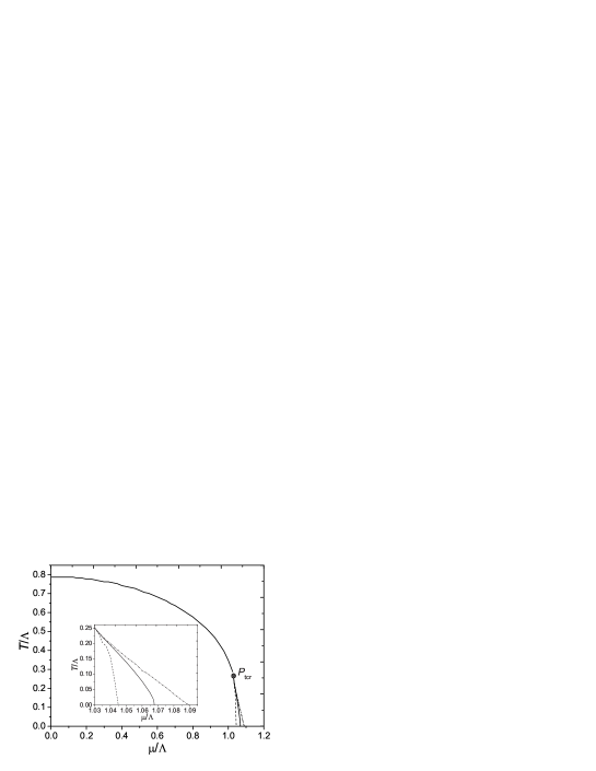
Figure 2: The phase diagram for $N=3$ obtained within the OPT. The position of the tricritical point is indicated by $P_{\rm tcr}$, where the second order transition line (above $P_{\rm tcr}$) turns into a first order one (below $P_{\rm tcr}$). CSB happens at the left of the continuous curve while CSR happens at the right hand side. The dashed and dot-dashed lines are the metastable lines running along the first order line. The inner plot zooms into the region around the first order transition line.

According to the large-$N$ approximation the discrete chiral transition in the GN model is of the second order everywhere except at $T=0$ and $\mu=\mu_{c}$. The results obtained from the OPT, however, show the existence of a tricritical point at $T_{\rm tcr}\simeq 0.25\Lambda$ and $\mu_{\rm tcr}\simeq 1.03\Lambda$ (for $N=3$), represented by the black dot in Fig. 2. Below this point the transition is of the first kind, while above it is of the second kind. Metastable lines can be found at the left and right of the first order critical curve on Fig. 2, running very close to it from the tricritical point down to the $\mu$ axis. Any method relying on determining this region, if not enough precise, is very likely to miss it. This may then possibly explain why previous works, most notably lattice Monte-Carlo simulations lattice2 , had difficulties to probe the possible existence of a mixed phase. It is possible to use the OPT-PMS in conjunction with Landau’s expansion in order to determine the tricritical points for any finite values of $N$. In this case one can just reinstate the chemical potential back in the last term of Eq. (7), iterate it to the desired order, substitute the solution back in the expression for the effective potential to then obtain the coefficients $a(\mu,T)$ and $b(\mu,T)$ in Eq. (11). Then by solving $a(\mu_{tcr},T_{tcr})=0$ and $b(\mu_{tcr},T_{tcr})=0$ simultaneously, the tricritical points can easily be extracted. As discussed above, direct numerical evaluation using the Eq. (4) and the PMS optimization give $T_{\rm tcr}\simeq 0.25\Lambda$ and $\mu_{\rm tcr}\simeq 1.03\Lambda$ for $N=3$. The Landau’s expansion, with for example the OPT-PMS2, gives $T_{\rm tcr}\simeq 0.24\Lambda$ and $\mu_{\rm tcr}\simeq 1.03\Lambda$. These results again compare very well with the full numerical results used to obtain Fig. 2. In Table II we present all the relevant results for chiral symmetry restoration for different values of $N$. The quantities $T_{c}$ (at $\mu=0$), $T_{tcr}$ and $\mu_{tcr}$ have been originally obtained in the present work using the Landau expansion within the next order iteration PMS2, as described above, while $\mu_{c}$ (at $T=0$) is given by the solution of Eq. (13) and the order parameter, ${\bar{\sigma}}_{c}$, is given by Eq. (9).

$N$	${\bar{\sigma}}_{c}$ ($T=\mu=0$)	$T_{c}$ ($\mu=0$)	$\mu_{c}$ ($T=0$)	$T_{tcr}$	$\mu_{tcr}$
1	1.78	0.96	1.24	0.46	1.06
3	1.19	0.79	1.07	0.24	1.034
4	1.14	0.77	1.05	0.21	1.03
6	1.09	0.75	1.03	0.19	1.02
10	1.05	0.74	1.02	0.17	1.01
$\infty$	1.0	0.72	1.0	0.0	1.0

Table 2: The relevant physical quantities (in units of $\Lambda$) for different values of $N$.

It is also possible to express and analyze the phase diagram in terms of the pressure $P$ and density $\rho$, defined respectively by $P=-V_{\rm eff}({\bar{\eta}},\bar{\sigma}_{c},\mu,T)$ and $\rho=\partial P/\partial\mu$. This was done in long , where it was shown the existence of a chiral broken/restored coexistence phase (the analog of a liquid-gas phase), whose result is a direct consequence of the existence of the tricritical point seen in Fig. 2. At this point one may wonder how the consideration of the order-$\delta^{2}$ terms, which contains additional $1/N$ as well as new $1/N^{2}$ corrections, would affect the first order results. Clearly, at $T\neq 0$ and $\mu\neq 0$ the explicit evaluation of all the three loop contributions is a rather difficult task. Nevertheless, at $T=0$ and $\mu=0$, a lengthy evaluation of those contributions has been done in Ref. long showing that the potential corrections to the ${\cal O}(\delta)$ results are not negligible but remain under control, about a few percent. For example, the result obtained for the scalar field vacuum expectation value at $T=0$ and $\mu=0$ is found to be (at $N=3$) ${\bar{\sigma}}_{c}\simeq 1.17\,\Lambda$ at ${\cal O}(\delta^{2})$, for a reasonable choice of the arbitrary renormalization scale, chosen as given by $\Lambda$, while at ${\cal O}(\delta)$ it is ${\bar{\sigma}}_{c}\simeq 1.19\,\Lambda$. For larger values of $N$ the difference gets even smaller, in conformity with the large-$N$ results (since at $N\to\infty$ the OPT converges exactly to the large-$N$ results LPR ). This then hints on the accuracy and quick convergence of the order-$\delta$ results discussed in this letter.

V Conclusions

In conclusion, by studying the 2+1 dimensional four-fermion GN model with discrete chiral symmetry in terms of the OPT, we have shown how this method can be advantageous compared to the widely used large-$N$ and Monte Carlo approximations. Here we have presented precise analytical expressions for the order parameter ${\bar{\sigma}}_{c}$ (at $T=\mu=0$), the critical temperature $T_{c}$ (at $\mu=0$), and the critical chemical potential $\mu_{c}$ (at $T=0$) for CSR which are valid for any values of $N$ already at lowest order in the OPT. As usual, all these relations exactly reproduce the standard large-$N$ results when the $N\to\infty$ limit is taken. We were also able to precisely locate a tricritical point in the $(T,\mu)$ phase diagram not seen using the large-$N$ approximation and also not obtained before using other methods, though numerical simulations seemed to indicate its presence. We have discovered that, due to the finite $N$ effects, the model behaves as a Van der Waals liquid in which a coexistent liquid-gas phase does exist. The observed metastable region is rather small, which possibly explains why its observation was missed in Ref. lattice2 and previous works. All these results seem to survive when going to higher orders in the OPT, as we discussed in the last section. In this letter we have extended our previous applications of the OPT to the Gross-Neveu model LPR ; long by analyzing how the method can be applied to the Landau expansion for the free energy density in order to determine the value of critical quantities in a way that is less time consuming than the straight numerical methods used in Refs. LPR ; long . We have shown that this is possible if one considers further approximations in the optimization equations. However, the numerical effects of such approximations, even at the first level, turn out to be negligible.

Concerning the next order OPT corrections we have checked in Ref. long that, for $T=0=\mu$, $N=3$, and a reasonable choice of renormalization scale the differences for the order parameter are about $2\%$. As for the $1/N$ expansion we are not in position to speculate what a complete next to the leading $1/N^{2}$ order calculation would give from a quantitatively perspective. However, we believe that it should point out to the existence of a tricritical point in the $T-\mu$ plane since, according to our work, this seems to be an effect of finite $N$ corrections which is also supported by Monte Carlo applications lattice1 ; lattice2 .

Possible follow-ups to this work that would be interesting to investigate regard the possible existence of a kind of nuclear matter state around $\mu_{c}$, at large $\mu$ and low $T$, for which the chiral phase would be degenerate with a baryonic phase, $\langle\bar{\psi}\psi\rangle\neq 0$ and $\langle\bar{\psi}\gamma_{0}\psi\rangle\neq 0$. This is still an unsettled question in the literature and that could be ideally addressed with the OPT. Another interesting work would be to evaluate the various critical (and tricritical) exponents, determining whether they belong to the mean-field universality class or the Ising universality class in two dimensions. This is also a controversial point concerning the GN model, with no clear answer so far in the literature. Based on its recent success in dealing with critical theories LPR ; moreOPT ; conv we expect that the method employed here will be a valuable tool in these analysis providing us with a better understanding of the chiral symmetry behavior in a hot and dense medium.

Finally, we point out that since the GN model is part of a larger class of four-Fermi models, e.g. the Nambu-Jona-Lasinio type of models commonly used in nuclear physics problems and as an effective model for QCD, or even its non-relativistic version, used in the study of planar superconductors and low dimensional fermionic systems (like Fermi gases in atomic physics), we expect that not only our results but also the OPT method used to obtain them can be of interest and have applications in these areas as well. In particular, we believe that the success of the OPT method in redrawing the phase diagram of the three dimensional GN model could certainly attract the attention of condensed matter as well as nuclear physicists to this method as an alternative tool to the well known large-$N$ and Monte Carlo techniques, which are currently used in an interdisciplinary manner.

- (1) D. Gross and A. Neveu, Phys. Rev. D10 (1974) 3235.
- (2) B. Rosenstein, B. J. Warr and S. H. Park, Phys. Rep. 205 (1991) 59.
- (3) I. J. R. Aitchison and N. E. Mavromatos, Phys. Rev. B53 (1996) 9321; R. Sharkar, Phys. Rev. Lett. 63 (1989) 203;
- (4) S. Christofi and C. Strouthos, arxiv: hep-lat/0612031; S. Hands, J. B. Kogut, C. G. Strouthos and T. N. Tran, Phys. Rev. D68 (2003) 016005 (2003); S. J. Hands, A. Kocić and J. B. Kogut, Nucl. Phys. B390 (1993) 355.
- (5) J. B. Kogut and C. G. Strouthos, Phys. Rev. D63 (2001) 054502.
- (6) S. Muroya, et al, Prog. Theor. Phys. 110 (2003) 615.
- (7) K. G. Klimenko, Z. Phys. C37 (1988) 457.
- (8) J. A. Gracey, Phys. Rev. D50 (1994) 2840;
- (9) V.I. Yukalov, Teor. Mat. Fiz. 28 (1976) 92; R. Seznec and J. Zinn-Justin, J. Math. Phys. 20 (1979) 1398; A. Okopińska, Phys. Rev. D35 (1987) 1835; A. Duncan and M. Moshe, Phys. Lett. B215 (1988) 352.
- (10) N. D. Mermin and H. Wagner, Phys. Rev. Lett. 17 (1966) 1133; S. Coleman, Comm. Math. Phys. 31 (1973) 259.
- (11) J.-L. Kneur, M. B. Pinto and R. O. Ramos, Phys. Rev. D74 (2006) 125020; Braz. J. Phys. 37 (2007) 258.
- (12) M. B. Pinto and R. O. Ramos, Phys. Rev. D60 (1999) 105005; ibid. D61 (2000) 125016; J.-L. Kneur, A. Neveu and M. B. Pinto, Phys. Rev. A69 (2004) 053624; S. K. Gandhi and M. B. Pinto, Phys. Rev. D49 (1994) 4258; S. K. Gandhi, H. F. Jones and M. B. Pinto, Nucl. Phys. B359 (1991) 429; C. Arvanitis, F. Geniet, M. Iacomi, J.-L. Kneur and A. Neveu, Int. J. Mod. Phys. A12 (1997) 3307; K. G. Klimenko, Z. Phys. C50 (1991) 477.
- (13) P.M. Stevenson, Phys. Rev. D23 (1981) 2916.
- (14) J.-L. Kneur, M. B. Pinto, R. O. Ramos and E. Staudt, arXiv:0705.0676.
- (15) J.-L. Kneur, M. B. Pinto and R. O. Ramos, Phys. Rev. Lett. 89 (2002) 210403; Phys. Rev. A68 (2003) 043615; J.-L. Kneur and D. Reynaud, Phys. Rev. D66 (2002) 085020.