Hyperbolicity of exact hydrodynamics for three-dimensional linearized Grad’s equations

Abstract

We extend a recent proof of hyperbolicity of the exact (to all orders in Knudsen number) linear hydrodynamic equations [M. Colangeli et al, Phys. Rev. E (2007)] to the three-dimensional Grad’s moment system. A proof of an $H$-theorem is also presented.

I Introduction

Derivation of hydrodynamics from a microscopic description is the classical problem of physical kinetics. The Chapman-Enskog method chapman derives the solution from the Boltzmann equation in a form of a series in powers of Knudsen number $\varepsilon$, where $\varepsilon$ is a ratio between the mean free path of a particle and the scale of variations of hydrodynamic fields. The Chapman-Enskog solution leads to a formal expansion of stress tensor and of heat flux vector in balance equations for density, momentum, and energy. Retaining the first order term ($\varepsilon$) in the latter expansions, we come to the Navier-Stokes equations, while next-order corrections are known as the Burnett ($\varepsilon^{2}$) and the super-Burnett ($\varepsilon^{3}$) corrections chapman .

However, as it was first demonstrated by Bobylev for Maxwell’s molecules bobylev1 , even in the simplest case (one-dimensional linear deviation from global equilibrium) the Burnett and the super-Burnett hydrodynamics violate the basic physics behind the Boltzmann equation. Namely, sufficiently short acoustic waves are increasing with time instead of decaying. This instability contradicts the $H$-theorem, since all near-equilibrium perturbations must decay. This creates difficulties for an extension of hydrodynamics, as derived from a microscopic description, into a highly non-equilibrium domain where the Navier-Stokes approximation is inapplicable.

Recently, Bobylev suggested a different viewpoint on the problem of Burnett’s hydrodynamics Bo2006 . Namely, violation of hyperbolicity can be seen as a source of instability. We remind that Boltzmann’s and Grad’s equations are hyperbolic and stable due to corresponding $H$-theorems. However, the Burnett hydrodynamics is not hyperbolic which leads to no $H$-theorem. Bobylev Bo2006 suggested to stipulate hyperbolization of Burnett’s equations which can also be considered as a change of variables. In this way hyperbolically regularized Burnett’s equations admit the $H$-theorem (in the linear case, at least) and stability is restored.

Inspired by this study, in our recent paper cokk (referred as CKK hereafter), we have considered the simplest nontrivial example - linearized Grad’s moment equation in one spatial dimension - and demonstrated that, upon a certain transformation, the exact (to all orders in Knudsen number) hydrodynamic equations are manifestly hyperbolic and stable. Thus, the first complete answer to what is the structure of the extended hydrodynamics was obtained.

In this paper, we extend the CKK result to three-dimensional linearized Grad’s equations. In addition we prove the existence of an $H$-function. The paper is organized as follows: In Sec. II, through a Dynamic Invariance Principle GK92 ; GK94 ; Ka2005 , we derive equations of linear exact hydrodynamics. In Sec. III we demonstrate that exact hydrodynamic equations are manifestly hyperbolic and dissipative. Then, In Sec. IV we stress explicitly how the stability of hydrodynamic equations, and therefore the existence of an $H$-theorem, arises as an interplay between these two basic ingredients of resulting hydrodynamics: dissipativity and hyperbolicity. Finally, a conclusion is given in Sec. V.

II Hydrodynamics from the linearized Grad system

II.1 Linearized Grad’s equations in $k$-space

The thirteen moments linear Grad system consists of 13 linearized PDE’s giving the time evolution of the hydrodynamic fields (density $\rho$, velocity vector field $u$, Temperature $T$) and of higher order distinguished moments: five components of the symmetric traceless stress tensor $\sigma$ and three components of the heat flux $q$ Grad .

Point of departure is the Fourier transform of the linearized three-dimensional Grad’s thirteen-moment system:

$$\partial_{t}\rho_{k} = -i\mbox{\boldmath{$k$}}\cdot\mbox{\boldmath{$u$}}_{k},$$ (1a)

$$\partial_{t}\mbox{\boldmath{$u$}}_{k} = -i\mbox{\boldmath{$k$}}\rho_{k}-i\mbox{\boldmath{$k$}}T_{k}-i\mbox{\boldmath{$k$}}\cdot\mbox{\boldmath{$\sigma$}}_{k},$$ (1b)

$$\partial_{t}T_{k} = -\frac{2}{3}i\mbox{\boldmath{$k$}}\cdot(\mbox{\boldmath{$u$}}_{k}+\mbox{\boldmath{$q$}}_{k}),$$ (1c)

$$\partial_{t}\mbox{\boldmath{$\sigma$}}_{k} = -2i{\hskip 1.99997pt\stackrel{{\scriptstyle\vrule width=0.2411pt,height=0.2411pt,depth=1.43161pt\hbox{\vrule width=10.8759pt,height=0.2411pt,depth=0.0pt}\vrule width=0.2411pt,height=0.2411pt,depth=1.43161pt}}{{\mbox{\boldmath{$k$}}\mbox{\boldmath{$u$}}_{k}}}\hskip 1.99997pt}-\frac{4}{5}i{\hskip 1.99997pt\stackrel{{\scriptstyle\vrule width=0.2411pt,height=0.2411pt,depth=1.43161pt\hbox{\vrule width=10.24474pt,height=0.2411pt,depth=0.0pt}\vrule width=0.2411pt,height=0.2411pt,depth=1.43161pt}}{{\mbox{\boldmath{$k$}}\mbox{\boldmath{$q$}}_{k}}}\hskip 1.99997pt}-\mbox{\boldmath{$\sigma$}}_{k},$$ (1d)

$$\partial_{t}\mbox{\boldmath{$q$}}_{k} = -\frac{5}{2}i\mbox{\boldmath{$k$}}T_{k}-i\mbox{\boldmath{$k$}}\cdot\mbox{\boldmath{$\sigma$}}_{k}-\frac{2}{3}\mbox{\boldmath{$q$}},$$ (1e)

where $k$ is the wave vector, $\rho_{k}$, $\mbox{\boldmath{$u$}}_{k}$ and $T_{k}$ are the Fourier components for density, average velocity and temperature characterizing deviations from the equilibrium state, respectively, and $\mbox{\boldmath{$\sigma$}}_{k}$ and $\mbox{\boldmath{$q$}}_{k}$ are the nonequilibrium traceless symmetric stress tensor (${\hskip 1.99997pt\stackrel{{\scriptstyle\vrule width=0.2411pt,height=0.2411pt,depth=1.43161pt\hbox{\vrule width=4.83986pt,height=0.2411pt,depth=0.0pt}\vrule width=0.2411pt,height=0.2411pt,depth=1.43161pt}}{{\mbox{\boldmath{$\sigma$}}}}\hskip 1.99997pt}=\mbox{\boldmath{$\sigma$}}$) and heat flux vector components, respectively. The overline bar denotes the traceless symmetric part of a 2nd rank tensor $a$, ${\hskip 1.99997pt\stackrel{{\scriptstyle\vrule width=0.2411pt,height=0.2411pt,depth=1.43161pt\hbox{\vrule width=4.54008pt,height=0.2411pt,depth=0.0pt}\vrule width=0.2411pt,height=0.2411pt,depth=1.43161pt}}{{\mbox{\boldmath{$a$}}}}\hskip 1.99997pt}\equiv\frac{1}{2}(\mbox{\boldmath{$a$}}+\mbox{\boldmath{$a$}}^{T})-\frac{1}{3}{\rm tr}(\mbox{\boldmath{$a$}}){\bf I}$ with unity matrix ${\bf I}$. The system (1) provides the time evolution equations for a set of hydrodynamic (locally conserved) fields $[\rho,\mbox{\boldmath{$u$}},T]$ coupled to the nonhydrodynamic fields $\sigma$ and $q$. The goal is to reduce the number of equations in (1) and to arrive at a closed system for the hydrodynamic fields only.

To this end, it is common practice to decompose the vectors and tensors into parallel (longitudinal) and orthogonal (lateral) parts with respect to the wave vector, because the fields are rotationally symmetric around any chosen direction $k$. We introduce a unit vector in the direction of the wave vector, $\mbox{\boldmath{$e$}}_{k}=\mbox{\boldmath{$k$}}/k$, $k=|\mbox{\boldmath{$k$}}|$, and the corresponding decomposition, $\mbox{\boldmath{$u$}}_{k}=u_{k}^{\|}\,\mbox{\boldmath{$e$}}_{k}+\mbox{\boldmath{$u$}}_{k}^{\perp}$, $\mbox{\boldmath{$q$}}_{k}=q_{k}^{\|}\,\mbox{\boldmath{$e$}}_{k}+\mbox{\boldmath{$q$}}_{k}^{\perp}$, and $\mbox{\boldmath{$\sigma$}}_{k}=\frac{3}{2}\sigma_{k}^{\|}{\hskip 1.99997pt\stackrel{{\scriptstyle\vrule width=0.2411pt,height=0.2411pt,depth=1.43161pt\hbox{\vrule width=11.68704pt,height=0.2411pt,depth=0.0pt}\vrule width=0.2411pt,height=0.2411pt,depth=1.43161pt}}{{\mbox{\boldmath{$e$}}_{k}\mbox{\boldmath{$e$}}_{k}}}\hskip 1.99997pt}+2\mbox{\boldmath{$\sigma$}}_{k}^{\perp}$, where $\mbox{\boldmath{$e$}}_{k}\cdot\mbox{\boldmath{$u$}}_{k}^{\perp}=0$, $\mbox{\boldmath{$e$}}_{k}\cdot\mbox{\boldmath{$q$}}_{k}^{\perp}=0$, and $\mbox{\boldmath{$e$}}_{k}\mbox{\boldmath{$e$}}_{k}:\mbox{\boldmath{$\sigma$}}_{k}^{\perp}=0$.

Upon inserting the above decomposition into (1), and using identities, ${\hskip 1.99997pt\stackrel{{\scriptstyle\vrule width=0.2411pt,height=0.2411pt,depth=1.43161pt\hbox{\vrule width=11.68704pt,height=0.2411pt,depth=0.0pt}\vrule width=0.2411pt,height=0.2411pt,depth=1.43161pt}}{{\mbox{\boldmath{$e$}}_{k}\mbox{\boldmath{$e$}}_{k}}}\hskip 1.99997pt}\cdot\mbox{\boldmath{$e$}}_{k}=(2/3)\mbox{\boldmath{$e$}}_{k}$, $\mbox{\boldmath{$e$}}_{k}\mbox{\boldmath{$e$}}_{k}:{\hskip 1.99997pt\stackrel{{\scriptstyle\vrule width=0.2411pt,height=0.2411pt,depth=1.43161pt\hbox{\vrule width=11.68704pt,height=0.2411pt,depth=0.0pt}\vrule width=0.2411pt,height=0.2411pt,depth=1.43161pt}}{{\mbox{\boldmath{$e$}}_{k}\mbox{\boldmath{$e$}}_{k}}}\hskip 1.99997pt}={\hskip 1.99997pt\stackrel{{\scriptstyle\vrule width=0.2411pt,height=0.2411pt,depth=1.43161pt\hbox{\vrule width=11.68704pt,height=0.2411pt,depth=0.0pt}\vrule width=0.2411pt,height=0.2411pt,depth=1.43161pt}}{{\mbox{\boldmath{$e$}}_{k}\mbox{\boldmath{$e$}}_{k}}}\hskip 1.99997pt}:{\hskip 1.99997pt\stackrel{{\scriptstyle\vrule width=0.2411pt,height=0.2411pt,depth=1.43161pt\hbox{\vrule width=11.68704pt,height=0.2411pt,depth=0.0pt}\vrule width=0.2411pt,height=0.2411pt,depth=1.43161pt}}{{\mbox{\boldmath{$e$}}_{k}\mbox{\boldmath{$e$}}_{k}}}\hskip 1.99997pt}=2/3$, we obtain the following two closed sets of equations for the longitudinal and lateral modes,

$$\partial_{t}\rho_{k} = -ik\,u_{k}^{\|},$$

$$\partial_{t}u_{k}^{\|} = -ik\rho_{k}-ikT_{k}-ik\sigma_{k}^{\|},$$

$$\partial_{t}T_{k} = -\frac{2}{3}ik(u_{k}^{\|}+q_{k}^{\|}),$$

$$\partial_{t}\sigma_{k}^{\|} = -\frac{4}{3}iku_{k}^{\|}-\frac{8}{15}ikq_{k}^{\|}-\sigma_{k}^{\|},$$

$$\partial_{t}q_{k}^{\|} = -\frac{5}{2}ikT_{k}-ik\sigma_{k}^{\|}-\frac{2}{3}q_{k}^{\|},$$ (2)

and

$$\partial_{t}\mbox{\boldmath{$u$}}_{k}^{\perp} = -ik\,\mbox{\boldmath{$e$}}_{k}\cdot\mbox{\boldmath{$\sigma$}}_{k}^{\perp},$$

$$\partial_{t}\mbox{\boldmath{$\sigma$}}_{k}^{\perp} = -ik{\hskip 1.99997pt\stackrel{{\scriptstyle\vrule width=0.2411pt,height=0.2411pt,depth=1.43161pt\hbox{\vrule width=12.43486pt,height=0.2411pt,depth=0.0pt}\vrule width=0.2411pt,height=0.2411pt,depth=1.43161pt}}{{\mbox{\boldmath{$e$}}_{k}\mbox{\boldmath{$u$}}_{k}^{\perp}}}\hskip 1.99997pt}-\frac{2}{5}ik{\hskip 1.99997pt\stackrel{{\scriptstyle\vrule width=0.2411pt,height=0.2411pt,depth=1.43161pt\hbox{\vrule width=11.8037pt,height=0.2411pt,depth=0.0pt}\vrule width=0.2411pt,height=0.2411pt,depth=1.43161pt}}{{\mbox{\boldmath{$e$}}_{k}\mbox{\boldmath{$q$}}_{k}^{\perp}}}\hskip 1.99997pt}-\mbox{\boldmath{$\sigma$}}_{k}^{\perp},$$

$$\partial_{t}\mbox{\boldmath{$q$}}_{k}^{\perp} = -ik\,\mbox{\boldmath{$e$}}_{k}\cdot\mbox{\boldmath{$\sigma$}}_{k}^{\perp}-\frac{2}{3}\mbox{\boldmath{$q$}}_{k}^{\perp}.$$ (3)

Equations (2) and (3) are a convenient starting point to derive closed equations for the hydrodynamic fields. To this end, the Chapman-Enskog method amounts to eliminating the time derivatives of the stress tensor and of the heat flux in favor of spatial derivatives of the hydrodynamic fields of progressively higher order. It had already been noted earlier Ka2005 that we can express the stress tensor and the heat flux vector linearly in terms of the locally conserved fields by introducing six, yet unknown, scalar functions $A(k),\dots,Z(k)$ for the longitudinal part:

$$\sigma_{k}^{\|} = ikAu_{k}^{\|}-k^{2}B\rho_{k}-k^{2}CT_{k},$$ (4a)

$$q_{k}^{\|} = ikX\rho_{k}+ikYT_{k}-k^{2}Zu_{k}^{\|},$$ (4b)

and, respectively, two functions $D(k)$ and $U(k)$ for the transversal component,

$$\mbox{\boldmath{$\sigma$}}_{k}^{\perp} = ikD{\hskip 1.99997pt\stackrel{{\scriptstyle\vrule width=0.2411pt,height=0.2411pt,depth=1.43161pt\hbox{\vrule width=12.43486pt,height=0.2411pt,depth=0.0pt}\vrule width=0.2411pt,height=0.2411pt,depth=1.43161pt}}{{\mbox{\boldmath{$e$}}_{k}\mbox{\boldmath{$u$}}_{k}^{\perp}}}\hskip 1.99997pt},$$ (5a)

$$\mbox{\boldmath{$q$}}_{k}^{\bot} = -k^{2}U\mbox{\boldmath{$u$}}_{k}^{\perp},$$ (5b)

where the expressions for the longitudinal components share their form with the one-dimensional CKK case. Note that the functions introduced should be regarded as exact summation of the Chapman-Enskog expansion which amounts to expanding these functions into powers of $k^{2}$ and deriving coefficients of this expansions from a recurrent (nonlinear) system, cf. CKK and Ka2005 ). We do not dwell on this here since we shall use a more direct way to evaluate functions $A,\dots,Z,D,U$ in the sequel.

Finally, using expressions (4) and (5) in (2), (3) and denoting as $x_{k}=(\rho_{k},u_{k}^{\|},T_{k},\mbox{\boldmath{$u$}}_{k}^{\perp})$ the vector of the hydrodynamical variables, the equations of hydrodynamics can be written in a compact form using a block-diagonal matrix ${\cal M}_{k}$,

$$\partial_{t}x_{k}={\cal M}_{k}\,x_{k},\qquad{\cal M}_{k}=\left(\begin{array}[]{cc}{\cal M}_{k}^{\|}&0\\ 0&{\cal M}_{k}^{\perp}\\ \end{array}\right),$$ (6)

with

$${\cal M}_{k}^{\|}=\left(\begin{array}[]{ccc}0&-ik&0\\ -ik(1\!-\!k^{2}B)&k^{2}A&-ik(1\!-\!k^{2}C)\\ \frac{2}{3}k^{2}X&-\frac{2}{3}ik(1\!-\!k^{2}Z)&\frac{2}{3}k^{2}Y\end{array}\right),$$ (7)

and

$${\cal M}_{k}^{\perp}=k^{2}D\left(\begin{array}[]{cc}1&0\\ 0&1\\ \end{array}\right),$$ (8)

where the unit matrix is written in an (arbitrarily) fixed basis in the two-dimensional subspace of vectors $\mbox{\boldmath{$u$}}_{k}^{\perp}$. As follows from an immediate comparison with CKK, and due to the apparently useful notation, the matrix ${\cal M}_{k}^{\|}$ providing the evolution of the longitudinal modes, is exactly identical with the corresponding matrix (denoted as $M$ in CKK) for the one-dimensional case, where lateral modes are absent. The twice degenerated transversal (shear) mode is decoupled from the longitudinal modes. As a direct consequence, also the invariance equations to be discussed next, which will provide us with a set of nonlinear algebraic equations for the unknown functions $A$–$Z$, divide into two sub-blocks which can be solved separately.

II.2 Invariance Equations

In order to evaluate functions $A,\dots,Z,D,U$, we make use of the dynamic invariance principle (DIP) GK92 ; GK94 ; Ka2005 . Making use of DIP in just the same way as for the one-dimensional case (CKK) leads to two independent sets of invariance equations for the functions $A(k)$–$Z(k)$. We find that the first set (six coupled quadratic equations for $A,B,C$ and $X,Y,Z$) is identical to the one already presented, cf. CKK, Eq. (17).

For the transversal modes, the invariance condition reads,

$$\frac{\partial\mbox{\boldmath{$\sigma$}}_{k}^{\perp}}{\partial\mbox{\boldmath{$u$}}_{k}^{\perp}}\cdot(-ik\mbox{\boldmath{$e$}}_{k}\cdot\mbox{\boldmath{$\sigma$}}_{k}^{\perp})=\partial_{t}\mbox{\boldmath{$\sigma$}}_{k}^{\perp},$$

$$\frac{\partial\mbox{\boldmath{$q$}}_{k}^{\perp}}{\partial\mbox{\boldmath{$u$}}_{k}^{\perp}}\cdot(-ik\mbox{\boldmath{$e$}}_{k}\cdot\mbox{\boldmath{$\sigma$}}_{k}^{\perp})=\partial_{t}\mbox{\boldmath{$q$}}_{k}^{\perp},$$ (9)

where the time derivative in the left hand side is evaluated by chain rule using $\partial_{t}\mbox{\boldmath{$u$}}_{k}^{\perp}$. Substituting the functions (5) into (9), and requiring that the invariance condition is valid for any $\mbox{\boldmath{$u$}}_{k}^{\perp}$, we derive two coupled quadratic equations for the functions $D$ and $U$ which can be cast into the following form:

$$15k^{4}D^{3}+25k^{2}D^{2}+(10+21k^{2})D+10=0,$$

$$U=-\frac{3D}{2+3k^{2}D}.$$ (10)

Solution of the cubic equation (10) with the initial condition $D(0)=-1$ matches the Navier-Stokes asymptotics and was found analytically for all $k$. This solution is real-valued and is in the range $D(k)\in[-1.04,0]$, whereas $U(k)\in[0,2.72]$. The functions corresponding to the longitudinal part of the system have been obtained numerically in CKK. Because $D$ and $U$ are real-valued, we show in Fig. 1 the real parts for all coefficients, while their nonvanishing imaginary parts still coincide with those shown in CKK Fig. 4.

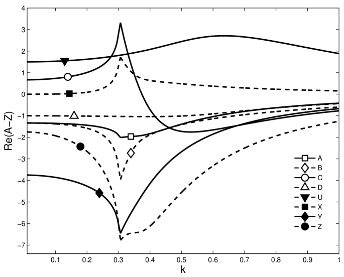
Figure 1: Real parts of coefficients $A$ to $Z$ solving the invariance equations, CKK (Eq. 17) supplemented with (10).

The dispersion relations $\omega(k)$ for the five hydrodynamic modes are then calculated by inserting these coefficients into the roots of characteristic equation ${\rm det}\left({\cal M}_{k}-\omega{\cal I}\right)=0$, where ${\cal I}$ is a $5\times 5$ unit matrix. Analogously, the dispersion relations for the remaining non-hydrodynamic modes follow from eight (remaining) eigenvalues of (2), (3) with (4), (5). All 13 modes are presented in Fig. 2. The resulting hydrodynamic spectrum consist of five modes: the acoustic mode, $\omega_{\rm ac}(k)$, represented by two complex-conjugated roots, the real-valued thermal (diffusive) mode, (both modes already occurring in the one-dimensional case) and a twice-degenerated real-valued shear mode (cf. Fig. 2). The occurrence of a real-valued shear mode confirms a more general result: in the linear regime, the shear mode never undergoes damped oscillations. Same as in the one-dimensional case, a critical point in the hydrodynamic spectrum occurs at $k_{c}\approx 0.303$, where the thermal mode intersects a non-hydrodynamical branch of the original Grad system. Hence, same conclusions hold here: for $k\geq k_{c}$, the CE method does not recognize any longer the resulting diffusive branch as an extension of a hydrodynamic branch. Figure 2 further shows the eight (all degenerated) non-hydrodynamic modes, which in opposite to the one-dimensional case (offering two non-hydrodynamic modes) also exhibit a critical $k$ at $k_{c}^{\prime}\approx 0.2175$.

To summarize, exact hydrodynamics as derived from invariance condition (or, equivalently, by the complete summation of the CE expansion as demonstrated in CKK (cf. also Ka2005 ) extends up to a finite critical value $k_{c}$, in full agreement with the one-dimensional case. No stability violation occurs, unlike in the finite-order truncations thereof. Next, we address the question about hyperbolicity of exact hydrodynamics in the present three-dimensional case.

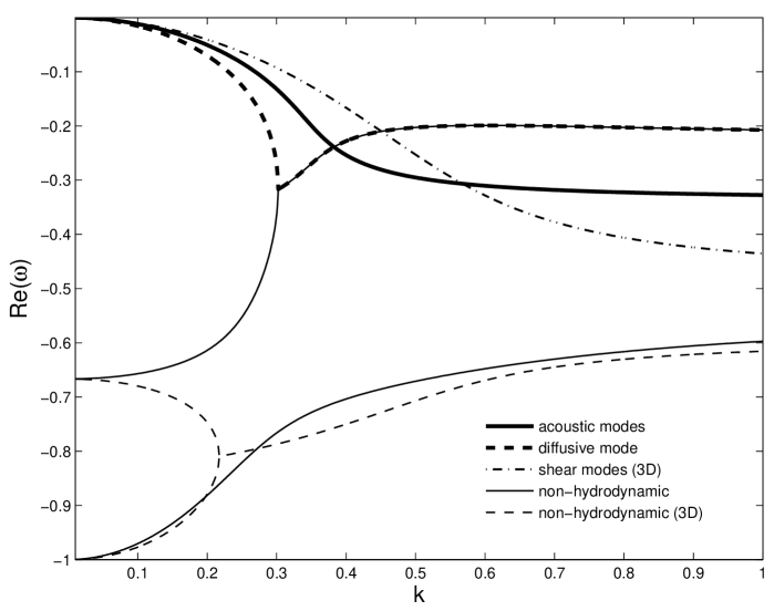
Figure 2: Dispersion relations $\omega(k)$ for the linearized Grad’s system using projected variables, Eqs. (2) and (3). The five hydrodynamic modes (diffusive, twice degenerated shear, and two complex-conjugated acoustic modes), as well as the eight non-hydrodynamic modes are presented as a function of $k$. While the acoustic mode is complex-valued for all $k$, the remaining modes become complex-valued beyond the two visible bifurcation points (at $k^{\prime}_{\rm c}\approx 0.2175$ and $k_{c}\approx 0.303$) For $k<k_{c}^{\prime}$ the non-hydrodynamic (3D) modes are degenerated two and four times, respectively, corresponding to the two and four components of $\mbox{\boldmath{$q$}}_{k}^{\perp}$ and $\mbox{\boldmath{$\sigma$}}_{k}^{\perp}$.

III Hyperbolicity of exact hydrodynamics

Distinguishing between the real (${{\cal R}}_{k}$) and imaginary (${{\cal I}}_{k}$) parts of matrix ${\cal M}_{k}$ (6), we can write the equation of hydrodynamics conveniently as

$$\partial_{t}x_{k} = [{{\cal R}}_{k}-i{{\cal I}}_{k}]\,x_{k},$$ (11)

$${{\cal R}}_{k}=\left(\begin{array}[]{cc}{\rm Re}({\cal M}_{k}^{\|})&0\\ 0&{\cal M}_{k}^{\perp}\\ \end{array}\right),\ -{{\cal I}}_{k}=\left(\begin{array}[]{cc}{\rm Im}({\cal M}_{k}^{\|})&0\\ 0&0\\ \end{array}\right).$$ (12)

The system (11) is hyperbolic and stable if we can find a transformation of the hydrodynamic fields, ${x}_{k}^{\prime}={\cal T}_{k}x_{k}$, where ${\cal T}_{k}$ is a real-valued matrix, such that, for the transformed matrices ${\cal M}_{k}^{\prime}={\cal T}_{k}{\cal M}_{k}{\cal T}_{k}^{-1}$ it holds

1. ${{\cal R}}^{\prime}_{k}={\rm Re}({\cal M}_{k}^{\prime})$ and ${{\cal I}}^{\prime}_{k}={\rm Im}({\cal M}_{k}^{\prime})$ are symmetric, and

2. ${{\cal R}}^{\prime}_{k}$ has non-positive eigenvalues.

Due to the block-diagonal structure of (6) as well as to the fact that CKK has solved the problem of finding a transformation with the desired properties for the one-dimensional case, the transformation exists also in the three-dimensional case, and has the following form:

$${\cal T}_{k}=\left(\begin{array}[]{cc}{\cal T}_{k}^{\|}&0\\ 0&{\cal T}_{k}^{\perp}\\ \end{array}\right),$$ (13)

where ${\cal T}_{k}^{\|}$ is explicitly given by CKK Eqs. (25)–(27) in terms of $k$, $A$–$C$ and $X$–$Z$, and

$${\cal T}_{k}^{\perp}=\left(\begin{array}[]{cc}1&0\\ 0&1\\ \end{array}\right).$$ (14)

Thus, the transformation ${\cal T}_{k}$ (13) symmetrizes ${\cal M}_{k}$ and renders the exact hydrodynamic equations manifestly hyperbolic. Furthermore, the transform ${\cal T}_{k}$ contains only even powers of $k$, because the same is true for the coefficients $A$–$Z$.

The five eigenvalues $\lambda_{1-5}$ of ${{\cal R}}^{\prime}_{k}$ (or, equally, of ${{\cal R}}_{k}$), are

$$\lambda_{1}=0,\;\;\;\lambda_{2}=k^{2}A,\;\;\;\lambda_{3}=\frac{2}{3}k^{2}Y,\;\;\;\lambda_{4,5}=k^{2}D.$$ (15)

From the analysis of the previous section, where we solved for coefficients $A$, $D$, and $Y$ appearing in (15), cf. Fig. 1, it follows that all the eigenvalues $\lambda_{1-5}$ are non-positive for all $k$. Note that the matrix ${{\cal R}}^{\prime}_{k}$ is diagonal with the diagonal elements (15).

IV H-theorem for exact hydrodynamics

Finally, the hyperbolic structure straightforwardly implies an $H$-theorem for the exact hydrodynamics (the same holds for any lower order approximation, if they are obtained according to the method presented in CKK). Note that, due to linearity of the system (1), the choice of a proper $H$-functional is not unique. We follow Bobylev Bo2006 , and consider an $H$-function – in terms of the transformed hydrodynamic fields – defined as:

$$H=\frac{1}{2}\int\left[\rho^{\prime 2}(\mbox{\boldmath{$r$}},t)+u^{\prime 2}(\mbox{\boldmath{$r$}},t)+T^{\prime 2}(\mbox{\boldmath{$r$}},t)\right]d^{3}r.$$ (16)

Here, hydrodynamic fields $x^{\prime}(\mbox{\boldmath{$r$}},t)$ are defined through inverse Fourier transform of the fields $x^{\prime}_{k}$. Note that $x^{\prime}(\mbox{\boldmath{$r$}},t)$ are real-valued because the real-valued transformation ${\cal T}_{k}$ is an even function of $k$, ${\cal T}_{k}={\cal T}_{-k}$. Therefore,

$$H=\frac{1}{2}\int\left[\rho^{\prime}_{k}\rho^{\prime}_{-k}+\mbox{\boldmath{$u$}}^{\prime}_{k}\cdot\mbox{\boldmath{$u$}}^{\prime}_{-k}+T^{\prime}_{k}T^{\prime}_{-k}\right]d^{3}k,$$ (17)

which we abbreviate as $H=\frac{1}{2}\left\langle{x}^{\prime}_{k},{x}^{\prime}_{-k}\right\rangle$. Thus,

$$\partial_{t}H = \frac{1}{2}(\left\langle x^{\prime}_{k},\partial_{t}x^{\prime}_{-k}\right\rangle+\left\langle\partial_{t}x^{\prime}_{k},x^{\prime}_{-k}\right\rangle)$$ (18)

$$= -\frac{1}{2}i(\left\langle x^{\prime}_{k},{{\cal I}}^{\prime}_{-k}x^{\prime}_{-k}\right\rangle+\left\langle x^{\prime}_{-k},{{\cal I}}^{\prime}_{k}x^{\prime}_{k}\right\rangle)$$

$$+\frac{1}{2}(\left\langle x^{\prime}_{k},{{\cal R}}^{\prime}_{-k}x^{\prime}_{-k}\right\rangle+\left\langle x^{\prime}_{-k},{{\cal R}}^{\prime}_{k}x^{\prime}_{k}\right\rangle).$$

Since ${{\cal I}}^{\prime}_{k}$ is an odd function of $k$, ${{\cal I}}^{\prime}_{-k}=-{{\cal I}}^{\prime}_{k}$, terms containing ${{\cal I}}^{\prime}$ cancel out, and we have, owing to the fact that ${{\cal R}}^{\prime}$ is even function of $k$ (${{\cal R}}^{\prime}_{-k}={{\cal R}}^{\prime}_{k}$),

$$\partial_{t}H=\sum_{s=1}^{5}\int\lambda_{s}|x^{\prime}_{s,k}|^{2}d^{3}k\leq 0.$$ (19)

Thus, we have proved the $H$-theorem for the exact hydrodynamics for $k<k_{c}$ (at $k=k_{c}$, the eigenvalues $\lambda_{2}$ and $\lambda_{3}$ become complex-valued, as discussed above).

V Conclusions

In this paper, we have considered derivation of exact hydrodynamics from linearized three-dimensional Grad’s system. The main finding is that the exact hydrodynamic equations (summation of the Chapman-Enskog expansion to all orders) are manifestly hyperbolic and stable, thereby extending the previous CKK result cokk . To the best of our knowledge, this is the first complete answer of the kind. The study supports the recent suggestion of Bobylev on the hyperbolic regularization of Burnett’s approximation. We have also demonstrated, by a direct computation, the $H$-theorem for the quadratic entropy function.

Acknowledgment

I.V.K. gratefully acknowledges support by BFE Project 100862 and by CCEM-CH. M.K. acknowledges support through grants NMP3-CT-2005-016375 and FP6-2004-NMP-TI-4 STRP 033339 of the European Community.

References

• (1) S. Chapman and T. G. Cowling, The Mathematical Theory of Nonuniform Gases (Cambridge University Press, New York, 1970).
• (2) A. V. Bobylev, Sov. Phys. Dokl. 27, 29 (1982).
• (3) A. V. Bobylev, J. Stat. Phys. 124, 371 (2006).
• (4) M. Colangeli, I. V. Karlin, and M. Kröger, Phys. Rev. E (2007) in press.
• (5) H. Grad, Comm. Pure and Appl. Math. 2, 331 (1949).
• (6) A. N. Gorban and I. V. Karlin, Physica A 190, 393 (1992).
• (7) A. N. Gorban and I. V. Karlin, Transport Th. Stat. Phys. 23, 559 (1994).
• (8) A. N. Gorban and I. V. Karlin, Invariant Manifolds for Physical and Chemical Kinetics, Lect. Notes Phys. 660 (Springer, Berlin, 2005).