Clustering Co-occurrences of Maximal Frequent Patterns in Streams

Abstract

One way of getting a better view of data is by using frequent patterns. In this paper frequent patterns are (sub)sets that occur a minimal number of times in a stream of itemsets. However, the discovery of frequent patterns in streams has always been problematic. Because streams are potentially endless it is in principle impossible to say if a pattern is often occurring or not. Furthermore, the number of patterns can be huge and a good overview of the structure of the stream is lost quickly. The proposed approach will use clustering to facilitate the “online” analysis of the structure of the stream.

A clustering on the co-occurrence of patterns will give the user an improved view on the structure of the stream. Some patterns might occur so often together that they should form a combined pattern. In this way the patterns in the clustering will approximate the largest frequent patterns: maximal frequent patterns. The number of (approximated) maximal frequent patterns is much smaller and combined with clustering methods these patterns provide a good view on the structure of the stream.

Our approach to decide if patterns occur often together is based on a method of clustering where only the distance between pairs of patterns is known. This distance is the Euclidean distance between points in a 2-dimensional space, where the points represent the frequent patterns, or rather the most important ones. The coordinates are adapted when the records from the stream pass by, and reflect the real support of the corresponding pattern. In this setup the support is viewed as the number of occurrences in a time window. The main algorithm tries to maintain a dynamic model of the data stream by merging and splitting these patterns. Experiments show the versatility of the method.

1 Introduction

Effectively mining streams of data with frequent patterns, i.e., patterns occurring at least a minimal number of times, has always been a hard problem to tackle. The difficulty lies in the fact that you don’t know which infrequent patterns suddenly will become frequent and standard ways of pruning the search space are nearly impossible to use. In this work patterns are sets of items occurring in a record (also called transaction or itemset) at a certain moment in time.

Example 1 Assume items $A$ and $B$ occur in every record, so they are frequent, and therefore also the itemset $\{A,B\}$ will be frequent. However in stream context we don’t know they are frequent. They may occur many times now and then never again.

Furthermore, if $\{A,B,C\}$ is not frequent, $\{A,B,C,D\}$ and all other possible additions to $\{A,B,C\}$ won’t be frequent either. This well-known anti-monotone property is difficult to use in streams since $\{A,B,C\}$ may not be frequent only for a short period. So $\{A,B,C\}$ in the stream as a whole might be frequent, but it doesn’t seem to be at the current moment since we have not seen all records. $\Box$

One interesting application of frequent patterns is that they can be used to get an overview of the structure of the dataset. Often there are too many patterns and further analysis of the patterns with for example clustering is useful, especially in the case of streams where the set of frequent patterns is always changing. We will propose a method of clustering where the distance between co-occurring maximal frequent subsets will be plotted in a 2-dimensional space. Maximal frequent subsets are sets of items occurring often in the stream while there is no frequently occurring bigger set of items containing these same items. Each of these maximal frequent subsets represents a branch of subsets occurring often together. If we combine this with information about the distance between the maximal frequent subsets, then we can provide interesting structural information about the stream. It will also possible to keep track of these sets in an online way.

We will define our method of clustering and show its usefulness. To this end, this paper makes the following contributions:
— We use a dynamic support estimation to determine the support of those itemsets we need, and do this in an online way.
— It will be explained how the distance between patterns is approximated, using the supports, by pushing and pulling. If this distance is large, patterns occur almost never together, and otherwise they do have many common occurrences.
— We will define when patterns can be merged and when they should be split to form smaller patterns and how this should be done. This could be considered as our major focus of interest.
— Finally through experiments the effectiveness of our clustering is shown and efficiency is discussed.

We first mention related work, then we discuss the algorithm in full detail. Finally we describe experiments and discuss these.

2 Related Work

This research is related to work done on clustering and in particular clustering in streams. Also our work is related to frequent (maximal) pattern mining in streams and large datasets.

There are many algorithms for mining maximal frequent patterns, in “normal” datasets, in different ways. We mention GenMax discussed in [9] and MAFIA presented in [3]. Large datasets are different from streams in that there is an end to the dataset. One approach to mining large datasets was proposed in [7], where an extremely large dataset is mined for maximal frequent patterns by proceeding in parallel. Furthermore clustering on large datasets was done in [14]. Much work has been performed on mining frequent patterns in (online) data streams, e.g., in [4] and [10]. In [5] frequent patterns are mined by using sliding window methods. Our work has little overlap with work done on maximal pattern-based clustering as discussed in [16] and [17] where objects basically are clustered by linking attribute groups with object groups when attributes have a minimal similarity. Related research has been done on clustering on streams in [1], where a study on clustering evolving data streams, (fast) changing data streams, is done. Aggarwal et al. continue their work in [2] by clustering text and categorical data in streams. Clustering categorical data was also done in [8] where also co-occurrence is used, but only for attribute values; the authors propose a visualization where the $x$-axis is the column position and the $y$-axis the distance based on co-occurrence of values. Also in [15] clustering on streams is mentioned, there the authors propose a new algorithm and compare it with K-Means (see [12]).

In this work a method of pushing and pulling points in accordance with a distance measure is used. This technique was used before in [6] to cluster criminal careers and was developed in [11]. This method of clustering was chosen since we only know the distance between two patterns, where a low distance means frequent co-occurrence. We don’t know the the precise $x$ and $y$ coordinates of the patterns, and therefore we cannot use standard methods of discovering clusters, e.g., K-Means.

3 The Algorithm:
Support and Distance,
Merge and Split

Our goal is to produce an algorithm that is capable of accepting a stream of records, each record being an unordered finite set of items, meanwhile building a model of the maximal frequent itemsets. The algorithm we propose, called DistanceMergeSplit, starts with randomly positioning $n$ points in a 2-dimensional space, e.g., in the unit square. Here $n$ is the number of items maximally possible in an itemset. Each of these $n$ points represents one size 1 itemset, where the size of an itemset is of course defined as the number of items it contains. These $n$ points remain present during the whole process, though their coordinates may change. While the records from the data stream pass by, new points are created (by merging or splitting) and others disappear (by merging, or by other reasons). Together these points constitute the evolving model $\cal{P}$, where points correspond with frequent itemsets.

We will first explain how we use the stream of records to update the supports of the elements of $\cal{P}$, we then present an outline of the algorithm; next we describe how the coordinates of the elements change in accordance with the corresponding supports, and finally mention our method of growing and shrinking the number of sets present in $\cal{P}$: the merge and split part of the algorithm.

3.1 Support

The algorithm will receive a possibly infinite stream of itemsets, the records: $r_{1},r_{2},r_{3},\ldots$ Each time an itemset corresponding to a point in the space is a subset of a record, we observe an occurrence of this itemset. We count the occurrences in the $m$ records we have seen so far (and that can also be considered as the last $m$ records), and define support:

$$\mathit{support\;(p,m)}=\sum_{t=1}^{m}\mathit{occurrence}\;(p,r_{t})$$ (1)

$$\mathit{occurrence}\;(p,r)=\left\{\begin{array}[]{l l}1&\quad\mbox{if $p\subseteq r$}\\ 0&\quad\mbox{otherwise}\\ \end{array}\right.$$

Here $\mathit{p}$ is the pattern, the itemset, for which support is computed, and $r$ is a record. If a new record arrives the support needs to be adapted accordingly. Rather than using the full support for all records, we will make use of a sliding window of size $\ell\geq 1$, and we will not keep the data about the occurrences of the patterns in the transactions of this window. Though this is not essential for our algorithm, it has a beneficial influence on the runtime, which is especially interesting for an online algorithm. If we have seen less than $\ell$ transactions ($m<\ell$) then we do use the previous formula to calculate support. This method will also be used when we later create new patterns online, and is referred to as “direct computation”; these patterns are then called “young”, as opposed to the “old” ones that are updated through equations 3.1 and 3.1 below. In the other case ($m\geq\ell$) we give an estimate $\mathit{support}_{t}(p)$ for the support during the last $\ell$ records in the following way. When the itemset $p$ is not a subset of the current record $r_{t}$ we adapt the support as follows:

$$\mathit{support}_{t+1}(p)$$

$$= \!\!\mathit{support}_{t}(p)/\ell\cdot(\mathit{support}_{t}(p)-1)$$

$$+\ (1-\mathit{support}_{t}(p)/\ell)\cdot\mathit{support}_{t}(p)$$

$$= \!\!(1-1/\ell)\cdot\mathit{support}_{t}(p)\;\leq\;\mathit{support}_{t}(p)$$

Indeed, when the first transaction of the window of size $\ell$ contains the pattern then support should decrease with 1. However, if the first record also does not contain $p$, then support remains the same. It is important to notice that the probability of a transaction containing $p$ in a window of size $\ell$ is estimated with $\mathit{support}_{t}(p)/\ell$. If the new record does contain the itemset $p$ then support is adapted as follows:

$$\mathit{support}_{t+1}(p)$$

$$= \!\!\mathit{support}_{t}(p)/\ell\cdot\mathit{support}_{t}(p)$$

$$+\ (1-\mathit{support}_{t}(p)/\ell)\cdot(\mathit{support}_{t}(p)+1)$$

$$= \!\!(1-1/\ell)\cdot\mathit{support}_{t}(p)+1\;\geq\;\mathit{support}_{t}(p)$$

Now when the first transaction of the window of size $\ell$ contains the pattern then support remains unchanged as the window shifts. However, if it does not contain the pattern $p$, then support will increase with 1. Both formulas assume that occurrences are uniformly spread over the window of size $\ell$, but by using these formulas to adapt support we do not have to keep all occurrences for all patterns in the 2-dimensional space. Notice that $0\leq\mathit{support}_{t}(p)\leq\ell$ always holds.

We have now described how the stream of records influences the supports of the itemsets that are currently being tracked, i.e., those in $\cal{P}$. Note that the itemsets of size 1 are always present in $\cal{P}$, for reasons mentioned in the next paragraph. Larger itemsets may appear and disappear as the algorithm proceeds. Also observe that the supports are estimates, due to the application of equations 3.1 and 3.1.

3.2 The Algorithm

The algorithm works with the set $\cal{P}$ of patterns that are currently present, represented by (coordinates of) points in 2-dimensional Euclidean space. The outline of the algorithm DistanceMergeSplit is as follows:  

initialize $\cal{P}$ with the $n$ itemsets of size 1
for $t\leftarrow 1$ to $\infty$ do
	$\cal{Q}\leftarrow\emptyset$
	for all patterns $p\in\cal{P}$ do
		compute $\mathit{support}_{t}(p)$ using the $t^{\mathrm{th}}$ record $r_{t}$,
		either through updating (old patterns)
		or by direct computation (young ones)
	for a random subset of pairs of patterns in $\cal{P}$ do
		update their distance according to their support
	for all “appropriate” pattern pairs in $\cal{P}$ do
		merge the pair, creating (new) pattern(s) in $\cal{Q}$
		mark the smallest of the pair,
		or both if their sizes are equal
	remove the marked patterns from $\cal{P}$
	for all patterns $p\in\cal{P}$ do
		if $p$ is infrequent and old enough then
			split $p$ into (new) patterns in $\cal{Q}$
			remove $p$ from $\cal{P}$
	${\cal{P}}\leftarrow\cal{P}\cup\cal{Q}$, joining duplicates
	remove non-maximal frequent patterns from $\cal{P}$

 

DistanceMergeSplit

 

Note that itemsets of size 1 are never removed from $\cal{P}$, not even when they are infrequent. The size 1 itemsets are always present, and play a special role: besides the fact that some of them are frequent, they also serve as building blocks. In many cases they are not maximal. If they were removed, it could be impossible to re-introduce single items after having become infrequent.

Patterns that are new in $\cal{P}$ are called “young”. When computing supports for these patterns, we use equation 1, when updating the “old” ones we use equations 3.1 and 3.1. So, each pattern present in $\cal{P}$ also has an age: patterns that have an age smaller than the window size $\ell$ are “young”, the others are “old”.

On two occasions the algorithm introduces indeterminism: first, when the support computation is done using the approximating updates for “old” patterns (saving a lot of time and memory) and second, when pushing and pulling a random subset of the pairs, see below.

3.3 Distance

We now describe how the coordinates of the points change as their supports vary when the new records from the stream come in. In our model for $\mathit{distance}\;(p_{1},p_{2})$ we take the Euclidean distance between the 2-dimensional coordinates of the points corresponding with the two patterns $p_{1}$ and $p_{2}$. These points are pulled closer to one another if they occur in the current transaction and they are pushed apart if not. Furthermore nothing is done if both do not occur. In every time step a random selection of the pairs undergoes this process.

To pull two points together we set the goal distance to 0 and to push them apart the goal distance is $\sqrt{2}$, which is the maximum Euclidean distance between any two points in the unit square. These distances are then used to update the coordinates $(x_{p_{1}},y_{p_{1}})$ and $(x_{p_{2}},y_{p_{2}})$ of the points:

1. $x_{p_{1}}\leftarrow x_{p_{1}}-\alpha\cdot(\mathit{distance}\;(p_{1},p_{2})-\gamma)\cdot(x_{p_{1}}-x_{p_{2}})$

2. $y_{p_{1}}\leftarrow y_{p_{1}}-\alpha\cdot(\mathit{distance}\;(p_{1},p_{2})-\gamma)\cdot(y_{p_{1}}-y_{p_{2}})$

3. $x_{p_{2}}\leftarrow x_{p_{2}}+\alpha\cdot(\mathit{distance}\;(p_{1},p_{2})-\gamma)\cdot(x_{p_{1}}-x_{p_{2}})$

4. $y_{p_{2}}\leftarrow y_{p_{2}}+\alpha\cdot(\mathit{distance}\;(p_{1},p_{2})-\gamma)\cdot(y_{p_{1}}-y_{p_{2}})$

Here $\alpha$ ($0\leq\alpha\leq 1$) is the user-defined learning rate and $\gamma$ ($0\leq\gamma\leq\sqrt{2}$) is the goal distance.

These formulas are basically the same as the one defined in [11], however we use the distances to decide when to merge. Points may leave the unit square; however, when presenting the results of the experiments, such points are projected on the nearest wall of this square.

3.4 Merge and Split

Now we describe how we merge and split the itemsets of the model as time goes by. The cluster model $\cal{P}$ contains points with corresponding itemsets. When the distance between two points is small, then the corresponding itemsets occur many times together. In some cases one itemset can be made that represents two of them: the algorithm will try these combinations. For some combinations it is possible that they turn out to be not so good, their frequency is smaller than $\mathit{minsupp}$, where $\mathit{minsupp}$ is a user-defined threshold. This can happen when their combined frequency is lower than $\mathit{minsupp}$ or suddenly frequency drops below $\mathit{minsupp}$. In either case we need to split the size $k$ itemset into $k$ itemsets of size $k-1$, all being subsets of the original itemset. Later we will discuss splitting in more detail, we now first explain merging.

As transactions come in, some of the initial size 1 itemsets become frequent, meaning that the support is higher than $\mathit{minsupp}$. These sets can — under certain circumstances, see below — merge to itemsets of size 2, and so on: two itemsets $p_{1}$ and $p_{2}$ are merged if (in the algorithm above the following series of conditions is referred to as “appropriate”):

• The two itemsets $p_{1}$ and $p_{2}$ currently are frequent, i.e., it holds that both $\mathit{support}_{t}(p_{1})\geq\mathit{minsupp}$ and $\mathit{support}_{t}(p_{2})\geq\mathit{minsupp}$. (Note that this condition automatically holds for all (pairs of) itemsets in $\cal{P}$ that have size larger than 1.)

• The itemsets are close together in the model, so they (probably) occur often together as a subset of transactions in the stream: $\mathit{distance}\;(p_{1},p_{2})\leq\mathit{mergedist}$, where $\mathit{mergedist}$ is a user-defined threshold for the distance between $p_{1}$ and $p_{2}$ below which merging is allowed.

• The pattern $p_{2}$ has an item $i_{p}$ which is not in the pattern $p_{1}$, such that $p_{2}\setminus\{i_{p}\}\subseteq p_{1}$. (This condition always holds if $p_{2}$ has size 1.)

• The patterns $p_{1}$ and $p_{2}$ are old enough: they exist in $\cal{P}$ for at least $\ell$ (the window size) records. (Note that the supports of these sets are currently updated through equations 3.1 and 3.1 above.)

If the patterns $p_{1}$ and $p_{2}$ are of equal size then for merging we create the set $p_{1}\cup p_{2}$. Both original patterns are removed from the 2-dimensional space except if their size is 1.

Example 2 Say $p_{1}=\{A,B,C\}$ and $p_{2}=\{A,B,D\}$. Furthermore, suppose $\mathit{distance}\;(p_{1},p_{2})=0.1$ and $\mathit{mergedist}=0.2$. Then the new itemset $q=\{A,B,C,D\}$ is added to the cluster model $\cal{Q}$ (and later to $\cal{P}$) with a randomly chosen $x$ and $y$ position. Both $p_{1}$ and $p_{2}$ are removed from $\cal{P}$ after all merging is done. It could be the case that $\{B,C,D\}$ and/or $\{A,C,D\}$ is infrequent, implying that $\{A,B,C,D\}$ will be infrequent too. However, in that case $\{A,B,C,D\}$ will disappear due to splitting; the patterns $p_{1}$ and $p_{2}$ should not have been so close together in the first place. $\Box$

If pattern $p_{1}$ contains more items than $p_{2}$ and $p_{2}\setminus\{i_{p}\}\subseteq p_{1}$ for some $i_{p}\in p_{2}$ with $i_{p}\not\in p_{1}$, then for each item $e\in p_{1}\setminus p_{2}$ we add an itemset $p_{2}\cup\{e\}$. This enables patterns to be merged with patterns that already were merged before and disappeared from the model. The smaller pattern $p_{2}$ is removed except if it is of size 1.

Example 3 Assume $p_{1}=\{A,B,C,D,E\}$, $p_{2}=\{A,B,F\}$, $\mathit{distance}\;(p_{1},p_{2})=0.1$ and $\mathit{mergedist}=0.2$. The algorithm will add $\{A,B,F,C\}$, $\{A,B,F,D\}$ and $\{A,B,F,E\}$ to $\cal{Q}$ (and later to $\cal{P}$). All $x$ and $y$ positions of the corresponding points are again randomly chosen. The itemset $p_{2}$ is removed from $\cal{P}$ after all merging is done, $p_{1}$ stays in $\cal{P}$. $\Box$

Next we split patterns, when they contain more than one item, if they do not occur often enough and they have been in the model for at least a certain number of records (they are “old enough”). Split combinations are generated by removing each item from the original pattern once. The remaining items form one new itemset, so in this way a size $k$ itemset will result in $k$ combinations after splitting.

Example 4 Assume $p=\{A,B,F\}$ has support $<\mathit{minsupp}$, and exists long enough in $\cal{P}$. The algorithm will add $\{A,B\}$, $\{A,F\}$ and $\{B,F\}$ to $\cal{Q}$ (and later to $\cal{P}$), located at random points. The itemset $p$ is removed from $\cal{P}$. $\Box$

Finally, the newly formed patterns in $\cal{Q}$ are united with those in $\cal{P}$. Of course, when patterns occur more than one time, only one copy — the oldest one — is maintained. And those patterns from $\cal{P}$ that are contained in a larger one in $\cal{P}$ are removed, unless — as stated above — they have size 1: we focus on the maximal patterns.

4 Experiments and Discussion

The experiments are organized such that we first show the method at work in a few controlled synthetic cases. Then we will use the algorithm to build a cluster model for a real dataset, showing some “real life” results. The first synthetic experiment will be a stream with 10 groups of 5 items. Groups do not occur together, but all of them occur often. This dataset is called the 10-groups dataset. The second synthetic experiment will be a stream where certain groups of items suddenly do not occur; instead another group starts occurring. We call this dataset the sudden change dataset. Finally one experiment will take the stream of the first experiment and it will test the effect of different noise levels; it will be called the noise dataset. The real dataset is the Large Soybean Database used for soybean disease diagnosis in [13]. The dataset contains 683 records with 35 attributes. First we removed all missing values and we converted each record to a string of $n=84$ yes/no values for each attribute value. In this research we do not deal with missing values, and each item represents an attribute value.

All experiments were performed on an Intel Pentium 4 64-bits 3.2 Ghz machine with 3 GB memory. As operating system Debian Linux 64-bits was used with kernel 2.6.8-12-em64t-p4.

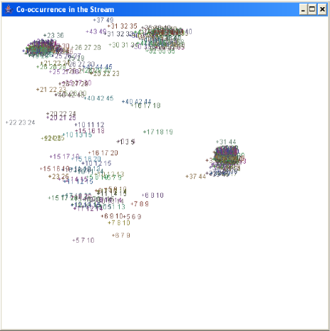
Figure 1: Model after seeing 600 transactions of the 10-groups dataset ($n=50$, $\mathit{minsupp}=15$, $\ell=\mathit{window\ size}=300$, $\mathit{mergedist}=0.1$, $\alpha=0.1$).

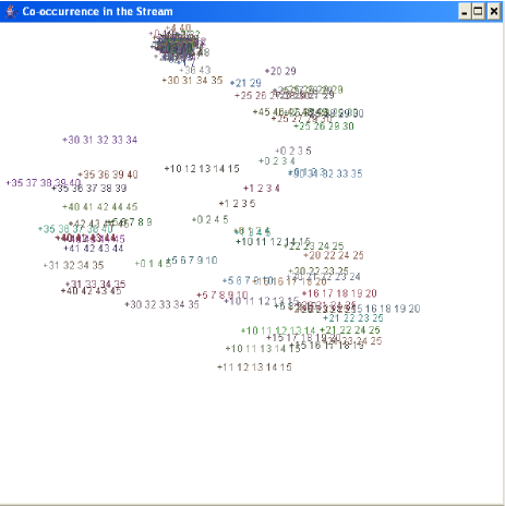
Figure 2: Model after seeing 1,200 transactions of the 10-groups dataset ($n=50$, $\mathit{minsupp}=15$, $\ell=\mathit{window\ size}=300$, $\mathit{mergedist}=0.1$, $\alpha=0.1$).

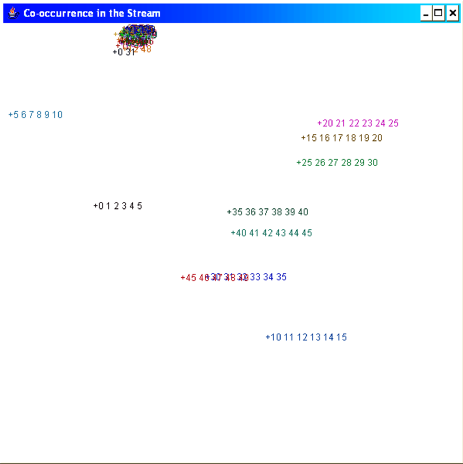
Figure 3: Model after seeing 4,500 transactions of the 10-groups dataset ($n=50$, $\mathit{minsupp}=15$, $\ell=\mathit{window\ size}=300$, $\mathit{mergedist}=0.1$, $\alpha=0.1$).

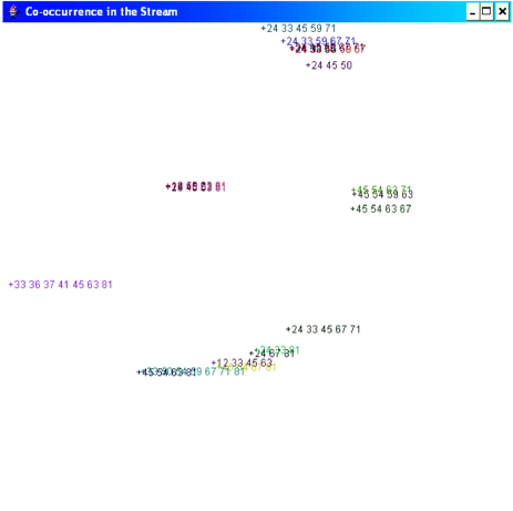
Figure 4: Model after 20,000 transactions of the real dataset were processed ($n=84$, $\mathit{minsupp}=120$, $\ell=\mathit{window\ size}=300$, $\mathit{mergedist}=0.1$, $\alpha=0.1$).

Figures 1, 2 and 3 show how the cluster model changes as more transactions are coming in for the 10-groups dataset. The first group of this dataset consists of items 0 to 5, the second has 5 to 10, etc. In the last figure, Figure 3, we clearly see these patterns. Furthermore notice that both the second and the first group contain the item 5, so there is a slight overlap. We see these itemsets closer together because they are both close to the pattern $\{5\}$. In order to get a clear picture we did not display the size 1 itemsets. Itemsets are plotted using $+$s, accompanied by the items they contain.

Figure 4 displays the cluster model (only patterns with age at least 50 are shown) after seeing 20,000 transactions produced by repeating the real dataset. Some patterns, i.e., itemsets, are clearly placed far apart from each other or close together. Table 1 displays some examples on the co-occurrences of patterns. The first thing to notice is that all the patterns occur often and so they should be in the cluster model. Secondly the first and the second itemset occur often together, so we expect them to be close together in the model. Finally the last itemset does not occur less often with the other two, we expect them to be placed further apart. Figure 4 displays all these facts in one picture.

	{24, 33, 81}	{24, 67, 81}	{24, 45, 50}
{24, 33, 81}	295/683	253/683	182/683
{24, 67, 81}	253/683	260/683	189/683
{24, 45, 50}	182/683	189/683	237/683

Table 1: Three patterns from the model of Figure 4 and their co-occurrence.

Figure 5: The root squared error between the real support and the approximated support in the time window for the real dataset ($n=84$, $\mathit{minsupp}=150$, $\ell=\mathit{window\ size}=300$, $\mathit{mergedist}=0.1$, $\alpha=0.1$).

Approximating supports well is important in order to know which itemsets should be split. In Figure 5 we show for all patterns in a computed cluster model, with a minimal age of 300, the error between their approximated support and their real support in the time window as the transactions from the real dataset arrive. The root mean squared error of the supports for this model is never larger than $0.045$. All supports are first made relative to the time window size by dividing by $300$.

Our cluster model is said to approach the maximal frequent patterns. In order to show that it is able to do so, we first extracted from the original real dataset (683 transactions) all maximal frequent patterns using the Apriori algorithm with $\mathit{minsupp}=341$, which corresponds to a relative support of $0.5$. Then we produced a model where $\ell=\mathit{window\ size}=1,000$, $\mathit{minsupp}=500$, $\mathit{mergedist}=0.1$ and $\alpha=0.1$. In Table 2 some statistics are shown.

Number of exactly matching patterns	19 out of 45
Number of patterns with zero or one
items extra	35 out of 45
Number of patterns not in the model	10 out of 45
Root squared error
for the relative support of	0.0176
matching maximal frequent patterns

Table 2: The approximation of the maximal frequent patterns in the real dataset after seeing 20,000 transactions ($n=84$, $\ell=\mathit{window\ size}=1,000$, $\mathit{minsupp}=500$, $\mathit{mergedist}=0.1$, $\alpha=0.1$).

Many of the maximal frequent patterns exist in the model, however the algorithm constantly tries extending itemsets based on an approximated distance. Because of this the model contains the maximal frequent patterns with an extra item. As a future improvement we might keep all itemsets until their superset is not young any longer. Only a few itemsets do not exist in the model, but many of their subsets were found. The root squared error for the 19 matching patterns is about $0.0176$.

Figure 6: The root squared error between the real support and the approximated support in the time window for the real dataset ($n=84$, $\mathit{minsupp}=500$, $\ell=\mathit{window\ size}=1,000$, $\mathit{mergedist}=0.1$, $\alpha=0.1$).

The bigger time window used in the experiment of Figure 6 shows a small improvement for the root squared error.

The second synthetic dataset, called the sudden change dataset, simulates a stream that completely changes after seeing many transactions (i.e., 30,000). The results are displayed in Figure 7, where the labels above each bar reveal the size of the itemsets. First the records in the stream always contain items 1 to 5. Then after 30,000 transactions they only contain items 25 to 30. Figure 7 shows how the first pattern appears and how it slowly disappears in the middle and in the end the model contains only the patterns with items 25 to 30.

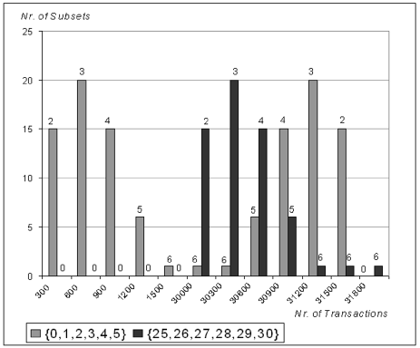
Figure 7: The sudden change dataset, the stream changes in the middle ($n=50$, $\mathit{minsupp}=15$, $\ell=\mathit{window\ size}=300$, $\mathit{mergedist}=0.1$, $\alpha=0.1$).

Finally Table 3 shows how noise influences the results. In the noise dataset each time a group of the same 11 items appears, first items 0 to 10, 10 to 20, etc. If the noise level is $r$ %, then approximately $r$ % of the items will not appear even though they should have. Table 3 shows that, even if there is noise, the correct itemsets are generated at least in part after seeing 50,000 transactions. We call an itemset correct if we would expect it. If a group contains items 0 to 10 then we would expect to see subsets with items 0 to 10. However unexpected would be to see itemsets with items 0 to 10 and some items outside this range. These unexpected subsets (subsets of all items in the group) did not occur often and their size was never bigger than 4 items.

Noise probability	Number of
of items (%)	expected subsets
0	5
10	3
20	28
30	19
40	10

Size range of	Number of
expected subsets	unexpected subsets
10 to 11 (items)	0
10 to 11	2
5 to 6	0
3 to 4	1
2 to 3	4

Table 3: The noise dataset, where the influence of noise on the structure is shown ($n=50$, $\mathit{minsupp}=15$, $\ell=\mathit{window\ size}=300$, $\mathit{mergedist}=0.1$, $\alpha=0.1$).

The processing time of the algorithm strongly depends on the support threshold $\mathit{minsupp}$ one chooses. The lower $\mathit{minsupp}$ is chosen the more points the cluster model will contain eventually and so processing time will get longer. Figure 9 shows that the average processing time for each transaction gets worse as the model contains more itemset points. However, Figure 9 shows that, for the real dataset, the number of points in the model eventually stabilizes. For each transaction we adapt the distances between points a number of times. In the case of the real dataset we randomly choose pairs 40,000 times in order to push or pull them, depending on their co-occurrence. Obviously one way of speeding up processing is to make it less than 40,000 times or one can skip adapting distances sometimes.

Figure 8: Transaction processing time in milliseconds for different cluster model sizes for the real dataset ($n=84$, $\mathit{minsupp}=60$, $\ell=\mathit{window\ size}=300$, $\mathit{mergedist}=0.1$, $\alpha=0.1$).

Figure 9: Development of cluster model size as transactions of the real dataset are processed ($n=84$, $\mathit{minsupp}=60$, $\ell=\mathit{window\ size}=300$, $\mathit{mergedist}=0.1$, $\alpha=0.1$).

5 Conclusions and Future Work

The algorithm presented in this paper will generate a cluster model of the maximal frequent itemsets and their co-occurrences. This gives the user a quick view on the patterns, frequent subsets, in the stream and how they occur in the stream. E.g., a shop keeper will know which products are often sold together and for the groups of products not often sold together the model indicates how much they are not sold together.

The co-occurrence distance of patterns is computed by pushing apart or pulling together patterns in a 2-dimensional space. Pushing was done when only one of the patterns occurs and pulling if they occur together. This distance is used to merge patterns together if it is smaller than a user-defined threshold, because we want only maximal frequent itemsets (itemsets that are often a subset of a transaction but they are never a subset of a bigger frequent itemsets) such that the model does not grow too big. Finally points are split if they happen to occur less than expected. Splitting and merging is required because the cluster model cannot contain all pattern since in streams we never know which items are frequent due to its possible infinite nature.

In the future we want to focus more on the applications of our algorithm and how it is best used in the analysis of streams. Furthermore we would like to examine how well the support estimates are, and how extra parameters (e.g., to determine the threshold age for splitting) can be employed.

6 Acknowledgment

This research is carried out within the Netherlands Organization for Scientific Research (NWO) MISTA Project (grant no. 612.066.304).

References

- [1] C. Aggarwal, J. Han, J. Wang, and P. Yu. A framework for clustering evolving data streams. In 29th International Conference on Very Large Data Bases (VLDB’03), pages 81–92, 2003.
- [2] C. Aggarwal and P. Yu. A framework for clustering massive text and categorical data streams. In SIAM Conference on Data Mining (SDM’06), pages 477–481, 2006.
- [3] D. Burdick, M. Calimlim, and J. Gehrke. MAFIA: A maximal frequent itemset algorithm for transactional databases. In 17th International Conference on Data Engineering (ICDE’01), pages 443–453, 2001.
- [4] J. Chang and W. Lee. Finding recent frequent itemsets adaptively over online data streams. In 9th ACM SIGKDD International Conference on Knowledge Discovery and Data Mining (KDD’03), pages 487–492, 2003.
- [5] J. Chang and W. Lee. estWin: Online data stream mining of recent frequent itemsets by sliding window methods. Journal of Information Science, 31(2):76–90, 2005.
- [6] J. de Bruin, T. Cocx, W. Kosters, J. Laros, and J. Kok. Data mining approaches to criminal career analysis. In 6th IEEE International Conference on Data Mining Proceedings (ICDM 2006), pages 171–177, 2006.
- [7] M. El-Hajj and O. Zaiane. Parallel leap: Large-scale maximal pattern mining in a distributed environment. In 12th International Conference on Parallel and Distributed Systems (ICPADS’06), pages 135–142, 2006.
- [8] D. Gibson, J. Kleinberg, and P. Raghavan. Clustering categorical data: An approach based on dynamical systems. In 26th International Conference on Very Large Data Bases (VLDB’00), pages 222–236, 2000.
- [9] K. Gouda and M. Zaki. Efficiently mining maximal frequent itemsets. In IEEE International Conference on Data Mining (ICDM’01), pages 163–170, 2001.
- [10] N. Jiang and L. Gruenwald. CFI-stream: Mining closed frequent itemsets in data streams. In 12th ACM SIGKDD International Conference on Knowledge Discovery and Data Mining (KDD’06), pages 592–597, 2006.
- [11] W. Kosters and M. van Wezel. Competitive neural networks for customer choice models. E-Commerce and Intelligent Methods of Studies in Fuzziness and Soft Computing, Physica-Verlag, Springer, 105:41–60, 2002.
- [12] J. MacQueen. Some methods for classification and analysis of multivariate observations. In 5th Berkeley Symp. Mathematical Statistics and Probability, pages 281–297, 1967.
- [13] R. Michalski and R. Chilausky. Learning by being told and learning from examples: An experimental comparison of the two methods of knowledge acquisition in the context of developing an expert system for soybean disease diagnosis. International Journal of Policy Analysis and Information Systems, 4(2):125–160, 1980.
- [14] A. Nanopoulos, Y. Theodoridis, and Y. Manolopoulos. C2P: Clustering based on closest pairs. In 27th International Conference on Very Large Data Bases (VLDB’01), pages 331–340, 2001.
- [15] L. O’Callaghan, N. Mishra, A. Meyerson, and S. Guha. Streaming-data algorithm for high-quality clustering. In 18th IEEE International Conference on Data Engineering (ICDE’02), pages 685–697, 2002.
- [16] J. Pei, X. Zhang, M. Cho, H. Wang, and P. Yu. MaPle: A fast algorithm for maximal pattern-based clustering. In 3th IEEE International Conference on Data Mining (ICDM’03), pages 259–266, 2003.
- [17] H. Wang, W. Wang, J. Yang, and P. Yu. Clustering by pattern similarity in large datasets. In SIGMOD International Conference (SIGMOD 2002), pages 394–405, 2002.