Radio Through X-ray Spectral Energy Distributions of 38 Broad Absorption Line Quasars

Abstract

We have compiled the largest sample of multiwavelength spectral energy distributions (SEDs) of Broad Absorption Line (BAL) quasars to date, from the radio to the X-ray. We present new Spitzer MIPS (24, 70, and 160µm) observations of 38 BAL quasars in addition to data from the literature and public archives. In general, the mid-infrared properties of BAL quasars are consistent with those of non-BAL quasars of comparable luminosity. In particular, the optical-to-mid-infrared luminosity ratios of the two populations are indistinguishable. We also measure or place upper limits on the contribution of star formation to the far-infrared power. Of 22 (57%) upper limits, seven quasars have sufficiently sensitive constraints to conclude that star formation likely contributes little ($<20\%$) to their far-infrared power. The 17 BAL quasars (45%) with detected excess far-infrared emission likely host hyperluminous starbursts with $L_{\rm fir,SF}=10^{13-14}$$L_{\odot}$. Mid-infrared through X-ray composite BAL quasar SEDs are presented, incorporating all of the available photometry. Overall, we find no compelling evidence for inherent differences between the SEDs of BAL vs. non-BAL quasars of comparable luminosity. Therefore a “cocoon” picture of a typical BAL quasar outflow whereby the wind covers a large fraction of the sky is not supported by the mid-infrared SED comparison with normal quasars, and the disk-wind paradigm with a typical radio-quiet quasar hosting a BAL region remains viable.

1. Introduction

Recent theoretical investigations into quasar feedback as a potentially important cosmological force in galaxy formation (e.g., Scannapieco & Oh, 2004; Granato et al., 2004; Springel et al., 2005; Hopkins et al., 2005) have led to a expansion of interest in quasar outflows. Energetic outflows are most obviously manifested in Broad Absorption Line (BAL) quasars. This population, approximately 20% (once selection effects are taken into account) of optically selected type 1 quasar samples (e.g., Hewett & Foltz, 2003; Reichard et al., 2003a), is notable for broad, blueshifted absorption evident in common ultraviolet resonance transitions such as C IV, Ly$\alpha$, and O VI. These P Cygni-type features arise because the observer is looking through an outflowing wind. Both the high velocities (up to 0.03 to 0.1$c$) and the relatively high ionization state of the gas indicate that the wind originates within the inner parsec of the central engine, and is likely more or less co-spatial with the broad-line region gas (Murray et al., 1995; Proga et al., 2000).

While the line of sight to an individual BAL quasar certainly cuts through an outflowing wind, the average covering fraction of the outflow remains difficult to constrain. For example, it may be that BAL quasars have a wind that covers a large fraction of the sky, and therefore only about 20% of quasars have BAL outflows. Alternately, most quasars may host BAL outflows, with the 20% (corrected) population fraction resulting from the average BAL wind covering fraction. The latter interpretation is supported by evidence from spectropolarimetry that there are absorption-line-free lines of sight in BAL quasars (e.g., Ogle et al., 1999), and the wind covering fraction is inferred to be low from constraints on ultraviolet emission-line scattering (Hamann et al., 1993). Weymann et al. (1991) found an overall similarity of BAL and non-BAL quasar ultraviolet-optical continuum and emission-line properties. More subtly, the significantly larger spectral comparison of Reichard et al. (2003b) revealed that BAL quasars are preferentially drawn from the non-BAL quasar population with intrinsically bluer continua, though they concluded that the parent populations of optically selected BAL and non-BAL quasars appear to be the same. At submm wavelengths, where the thermal dust emission is generated on much larger scales than the accretion disk, the populations of BAL and non-BAL quasars have indistinguishable flux distributions, though the majority of both populations have only upper limits (Lewis et al., 2003; Willott et al., 2003; Priddey et al., 2007). These empirical results are consistent with the disk-wind paradigm whereby a radiatively driven, equatorial wind from the accretion disk gives rise to both the broad emission and broad absorption-line features (Murray et al., 1995). However, a near-equatorial line of sight has been called into question by radio observations where typical orientation indicators (e.g., steep vs. flat radio spectra, and core vs. lobe-dominated flux ratios) suggest a range of inclination angles for radio-loud BAL quasars (Becker et al., 2000; Zhou et al., 2006; Brotherton et al., 2006). Furthermore, the identification of a few BAL quasars with ultra-luminous infrared galaxies (ULIRGS; e.g., Canalizo & Stockton, 2001) has led to the interpretation that BAL quasars may be “cocooned” during an obscured evolutionary stage in the transition from galaxy merger to starbursting ULIRG to shrouded BAL quasar to naked quasar (e.g., Sanders et al., 1988; Gregg et al., 2002).

The apparently contradictory results of these studies have led us to undertake a systematic survey of a well-defined sample of BAL quasars drawn from the Large Bright Quasar Survey (LBQS; Hewett et al., 1995; Hewett & Foltz, 2003). The goal is to obtain multiwavelength coverage of a sizable number of BAL quasars for comparison of the spectral energy distributions (SEDs) of BAL and non-BAL quasars in an effort to investigate the underlying relationship between the two populations. To date, there are two notable differences between BAL and non-BAL quasar SEDs: (1) BAL quasars typically show more evidence for dust reddening and extinction in their ultraviolet-optical spectra (Sprayberry & Foltz, 1992; Richards et al., 2002; Reichard et al., 2003b; Trump et al., 2006), and (2) BAL quasars are remarkably weak X-ray emitters (e.g., Green & Mathur, 1996; Gallagher et al., 2006). However, both of these properties are consistent with orientation-dependent obscuration effects.

In this present study, we focus on incorporating near and mid-infrared photometry into the picture, as longer wavelength data are expected to be less sensitive to absorption and less influenced by orientation effects. In particular, we will test the conclusion of Krolik & Voit (1998) that limb-darkening of the accretion disk emission should lead BAL quasars to have relatively weak ultraviolet-optical continua compared to non-BAL quasars if the BAL outflow is strongly equatorial. Goodrich (1997) reached a similar conclusion, though the proposed mechanism was orientation-dependent attenuation (perhaps via electron scattering) based on polarization studies. The ultraviolet-optical emission in quasars is generated by the accretion flow near the black hole, while infrared continuum light longward of $\sim 1$ µm is generally attributed to a parsec-scale, cold, and dusty region that is heated by and reprocesses the higher energy, direct continuum. Therefore, the mid-infrared power in BAL quasars should provide an independent measure of the intrinsic accretion luminosity to test these hypotheses.

Throughout we assume $\Lambda$-CDM cosmology with $\Omega_{\rm M}=0.3$, $\Omega_{\Lambda}=0.7$, and $H_{0}=70$ km s^-1 Mpc^-1 (Spergel et al., 2003, 2007).

2. Sample Selection

This sample was drawn from the Large Bright Quasar Survey (Hewett et al., 1995) sample of BAL quasars identified by Hewett & Foltz (2003). Each object has a BAL probability of 1.0 and $z>1.4$, the redshift at which the definitive C IV BAL is shifted into the wavelength regime accessible with ground-based spectroscopy. Of the 44 total BAL quasars meeting these criteria identified by Hewett & Foltz (2003), 38 were chosen for Spitzer 24, 70, and 160µm MIPS observations; we present this MIPS sample in this paper. The MIPS targets were chosen to maximize the available multiwavelength coverage. In addition to the mid and far-infrared coverage, available data archives and literature were searched to augment the multiwavelength photometry as much as possible. The targets are optically bright with $B_{J}$ magnitudes of 16.68–18.84, and they are drawn from a homogeneous, magnitude-limited quasar survey that has effective, well-defined, and objectively applied selection criteria (e.g., Hewett et al., 2001); six known BAL quasars with low-ionization (Mg II and/or Al III) BALs (hereafter, LoBALs) are included. The overall sample is luminous, with $M_{B}$ of –26.2 to –28.3 (using the K-corrections for non-BAL quasars of Cristiani & Vio 1990).

Our observed MIPS sample is listed in Table 1 including the redshift and BAL type. The classifications are HiBAL (no Al III or Mg II BAL detected), LoBAL (Mg II BAL detected), and Unknown (the electronic spectra do not cover Mg II).

3. Multiwavelength Photometry

The foundation of this multiwavelength SED project is complete mid and near-infrared photometry from Spitzer MIPS and the Two Micron All Sky Survey (2MASS; Skrutskie et al., 2006) of 38 LBQS BAL quasars. These data have been supplemented by near-complete (35 of 38) 0.5–8.0 keV X-ray data, multiband optical photometry for all, submm coverage for 16 objects, and Very Large Array (VLA) radio observations of 35 out of 38. In this section, the provenance of the SED data is briefly described.

3.1. Spitzer MIPS Photometry

The bulk of the MIPS data is the 36 BAL quasar observations from the Cycle 1 Director’s Discretionary Time for Gallagher’s Spitzer Fellowship program. Two additional objects, 0059$-$2735 and 1331$-$0108, are added from Program #82 (PI Rieke) of Cycle 1 Guaranteed Time.

The MIPS observation modes were one 3 s cycle at 24µm (48 s integration), one 3 s or 10 s cycle at 70µm (38 or 128 s integration), and four 10 s cycles at 160µm (84 s integration). The longer 70µm integration times were chosen for fainter sources, and the 160µm integration times were chosen to reach the confusion limit. All BAL quasars were detected with high S/N at 24µm. We consider BAL quasars with S/N$>3$ to be detected at 70 and 160µm. The upper limits are calculated as the flux in the source aperture + 3$\sigma$ or 3$\sigma$, whichever is greater (following the convention of the MIPS instrument team), where $\sigma$ is the standard deviation in the mean background. By this criterion, 13 BAL quasars are detected at 70µm, and three are detected at 160µm. (The two Guaranteed Time targets do not have 160µm coverage.) The Spitzer photometry is presented in Table 2.

3.2. Near-infrared

Thirty-two out of 38 BAL quasars are included in the 2MASS Point Source Catalog (PSC; Skrutskie et al., 2006); of these, all had $JHK$ detections except for 00211$-$0213, 1133$+$0214, 1314$+$0116, and 2116$-$4439, which only have upper limits in $K$. To obtain photometry (either upper limits or detections) for the remaining six (0051$-$0019, 1208$+$1535, 1240$+$1607, 1243$+$0121, 1443$+$0141, and 2140$-$4552), we downloaded the best Atlas $JHK$ images (recommended for photometry) from the 2MASS database. These images have all been flux-calibrated, combined, and resampled to a 1″/pixel scale; the photometric zeropoints are included in the fits image headers. We measured the signal (in data numbers) within a 2″-radius circular source cell centered on the LBQS optical position; the background was determined from an encircling annulus with inner and outer radii of 8″ and 10″, respectively. The noise per pixel, $\sigma$, is the standard deviation in the mean background. If the S/N within a 2″ aperture was more than 2.5, we consider the source to be detected. Otherwise, the upper limit is set to the 3$\sigma$ background level within the source cell area.

While a 2″ source cell maximized the S/N, a significant fraction of the flux in the point spread function is distributed outside of this aperture. To determine the aperture correction (which varies from field to field and band to band), we performed aperture photometry on the 2MASS PSC catalog sources with ‘AAA’ photometric quality flags and no galaxy contamination within 300″ of the target that coincided with the Atlas image area. The aperture correction for each target in each band was then the mean difference between the catalog magnitudes and their corresponding 2″-aperture magnitudes. The number of point sources used in the aperture correction determination was between four and 16; aperture correction values ranged from $-0.42$ to $-0.57$ magnitudes. The aperture correction was added to both the detections and upper limits to give the fluxes (converted to mJy from magnitudes) listed in Table 3. The standard deviation in the mean aperture correction has been folded into the photometric error.

Following the procedure outlined above, we obtain 37/35/32 detections in the $J$/$H$/$K$ bands, respectively, for the 38 objects in the sample.

3.3. X-ray

Thirty-four of the 38 objects in the sample were observed with Chandra, and a detailed analysis of these data and comparison with ultraviolet spectroscopic properties is presented in Gallagher et al. (2006). In addition, 2212$-$1759 was observed for 172 ks with XMM-Newton (Clavel et al., 2006). Using the 0.5–2.0 keV EPIC-pn count-rate upper limit ($<9.25\times 10^{-5}$ count s^-1), and assuming a power-law spectral index of $\alpha_{\rm X}=0.0$ (appropriate for absorbed sources), the modeling tool WebPIMMS gives $f_{\rm 2keV}<4.12\times 10^{-34}$ erg cm^-2 s^-1 Hz^-1.

In Table 3, the observed-frame 1 keV photometry is listed in units of $10^{-6}$ mJy for the 35 sources with X-ray data. The asymmetric flux errors result from Poisson X-ray counting statistics.

3.4. Optical

We have cross-correlated the LBQS Spitzer BAL quasar sample with the SDSS Data Release 5 archive. Of the 38 MIPS-observed BAL quasars, 22 have available SDSS photometry. We list the dereddened (for Galactic extinction) $ugriz$ PSF magnitudes for these objects in Table 3 converted to units of mJy using the SDSS zeropoint of 3631 Jy.

To obtain constraints on the optical colors of the remaining quasars, we convolved the electronic spectra (from Korista et al. 1993 [preferred] or Hewett et al. 1995) with the SDSS $gri$ filter functions for those quasars without SDSS coverage after first normalizing the available spectra using the LBQS $B_{J}$ photometry and transmission curves (Appendix A; Maddox & Hewett, 2006). These synthetic broad-band fluxes are presented in Table 3 (in units of mJy), errors are propagated from the 0.15 mag $B_{J}$ uncertainty (Hewett et al., 1995). The quoted uncertainty does not include additional errors from the convolution. The number of bandpasses is limited to the wavelength coverage of the electronic spectra.

To check on the absolute photometric accuracy of the synthetic fluxes, synthetic SDSS photometry was calculated for those quasars with actual SDSS data using non-SDSS electronic spectra. In sum, the average offsets between the synthetic and SDSS $gri$ photometry (defined as (SDSS – synthetic)/SDSS [mJy]) are within the 15% photometric uncertainty of the LBQS. The mean offsets and standard deviations of the mean offsets for $g$, $r$, and $i$ are $0\pm 27\%$, $-5\pm 37\%$, and $-12\pm 33\%$, respectively. The large standard deviations likely indicate that the synthetic photometric errors are underestimated, however, there is no evidence for absolute, systematic offsets between the synthetic and SDSS photometry.

3.5. Submillimeter

Sixteen of the 38 BAL quasars have been observed at 450 and 850µm with the Submillimetre Common-User Bolometer Array (SCUBA) instrument at the James Clerk Maxwell Telescope. The SCUBA data reduction and analysis is described in detail in Priddey et al. (2007). In this paper, we use $S/N\geq 2.5$ as the detection criterion; at 850µm (450µm), this yields five (two) detections with a 1$\sigma$ limit of $\sim 1.5$ mJy. A more conservative 3$\sigma$ threshold reduces the number of 850µm detections to three. For non-detections, the upper limits are given as the flux in the source aperture + $2\sigma$ or $2\sigma$, whichever is greater. The available photometry is included in Table 2.

3.6. Radio

Radio coverage is publicly available for 35 of 38 BAL quasars. These data are compiled from Stocke et al. (1992) (5 GHz), the Faint Images of the Radio Sky at Twenty cm (FIRST; White et al., 1997) (1.4 GHz), and the National Radio Astronomical Observatory VLA Sky Survey (NVSS; Condon et al., 1998) (1.4 GHz). Data are listed in Table 2. Upper limits for the FIRST survey are as given for the field in the catalog search; NVSS upper limits are 5 mJy (Condon et al., 1998).

Only one of the quasars in our sample, 2211$-$1915, is known to be formally radio-loud as defined by a radio luminosity of $>10^{32}$ erg s^-1 Hz^-1. The three quasars without radio constraints are too far south for the VLA. Based on the radio-loud fraction of the LBQS determined from a cross-correlation with the FIRST survey (Hewett et al., 2001), we expect at most 12% ($<1$) of these to be radio-loud, although a more likely value is 6% based on the lower fraction of radio-detected BAL versus non-BAL quasars (Hewett & Foltz, 2003).

4. Results and Discussion

We present the available multiwavelength photometry for each BAL quasar in Tables 2 and 3. The SED of each quasar is plotted in Figures 1a–1f in rest-frame units of $\log(\nu l_{\nu})$ ( erg s^-1) vs. $\log(\nu)$ (Hz), where $\log(\l_{\nu})$ includes the bandpass correction: $\log(f_{\nu})-\log(1+z)+\log(4\pi d_{\rm lum}^{2})-26$ ($f_{\nu}$ in mJy and luminosity distance, $d_{\rm lum}$, in cm). For reference, composite SEDs normalized to the 24µm MIPS data points are overlaid. The composite SEDs are the Elvis et al. (1994) mean SED at $\log(\nu)<13.57$ (8µm) and the Richards et al. (2006) luminous mean quasar SED for $\log(\nu)=12.50$–17.00 (95µm to 0.4 keV). For the $>0.5$ keV X-ray region, a spectral index of $\alpha_{\nu}=-1.0$ has been assumed (e.g., Gallagher et al., 2002; Page et al., 2005), with the normalization fixed by the best-fitting relation from Steffen et al. (2006, eq. 1c): $\log(l_{\rm 2keV})=0.721\log(l_{\rm 2500})+4.531$. This accounts for the empirical observation that the most ultraviolet-luminous quasars emit relatively less power in X-rays. From a qualitative inspection of the SEDs, the most obvious discrepancy between the plotted composites and the data is the known deficit at X-ray wavelengths when compared to the expected X-ray power.

To investigate the nature of mid-infrared SEDs of BAL quasars, a comparison sample is necessary. Given the known SED changes of normal type 1 quasars with luminosity in the X-ray (e.g., Avni & Tananbaum, 1986; Strateva et al., 2005; Steffen et al., 2006) and infrared regimes (Richards et al., 2006; Gallagher et al., 2007), identifying a comparison sample of objects with comparable luminosity is clearly preferred. The largest sample of quasar SEDs to date was presented by Richards et al. (2006) who incorporated the publicly available Spitzer MIPS+IRAC photometry as of the Data Release 3 quasar catalog of Schneider et al. (2005). All 259 objects were detected by Spitzer. We draw our comparison from the radio-quiet subset of this sample matched in monochromatic 5000Å luminosity to the LBQS BAL quasar sample ($\log(l_{\rm 5000\AA})=31.21$–32.29); a total of 40 objects. This luminous quasar sample is referred to as the SDSS comparison sample hereafter. While ideally the comparison sample would be drawn from the LBQS itself to mitigate possible selection effects, sensitive multiwavelength data as required for the comparison do not exist elsewhere. Luminous quasars are quite rare, and so accumulating a sizable sample (of order tens) requires multiwavelength, large area surveys or explicit targeting.

To compare directly the LBQS BAL quasar sample with the SDSS comparison sample, we compute three fiducial monochromatic luminosities at rest-frame 8µm, 5000Å, and 2500Å. The first is measured by normalizing the Richards et al. (2006) luminous ($\log(L_{\rm bol})>46.02$ erg s^-1) quasar composite SED to the 24µm MIPS datapoint. The second two are calculated from the best-fitting normalization, $l_{\nu,0}$, and spectral index, $\alpha_{\rm o}$, of a power-law model fit to the available rest-frame 1200–5000Å photometry: $l_{\nu}=l_{\rm\nu,0}\nu^{\alpha_{\rm o}}$. The lower frequency bound for this ultraviolet-optical bandpass is chosen to avoid the optical spectral region of $\lambda>5000$Å ($\nu<10^{14.78}$ Hz) where host-galaxy contamination can be significant (Vanden Berk et al., 2001); at $\lambda<1200$Å($\nu>10^{15.40}$ Hz), the intervening Ly$\alpha$ forest affects the spectra considerably. For the BAL quasars, the parameters, $\alpha_{\rm o}$, $\log(l_{\rm 8\mu{m}})$, $\log(l_{\rm 5000\AA})$, and $\log(l_{\rm 2500\AA})$, are listed in Table 1 along with $\log(l_{\rm 2keV})$ for those with X-ray data.

For reference, two integrated infrared luminosities, $L_{\rm ir,QSO}$ (1mm to 2µm) and $L_{\rm fir,QSO}$ (1mm to 20µm), are calculated using $l_{\rm 8\mu{m}}$ and the composite SEDs of Elvis et al. (1994) (for $\lambda\geq 40$µm) and Richards et al. 2006 (for $\lambda<40$µm). Elvis et al. (1994) (which used IRAS data) has better coverage at longer wavelengths, though we point out that neither composite is empirically constrained in the range from $\log(\nu)=10.2$–12.5 (16 GHz to 95µm). Using the combined composite SED, the infrared and far-infrared bolometric corrections from $\nu$$l_{\rm 8\mu{m}}$ to $L_{\rm ir,QSO}$ and $L_{\rm fir,QSO}$ are 2.99 and 0.84, respectively. Given that the near and mid-infrared emission is believed to be dominated by the quasar, these integrated infrared luminosities (normalized at rest-frame $\sim 8$µm) may be considered an estimate of the quasar’s contribution to the infrared SED. Any additional power in this regime could therefore be attributed to star-formation in the host galaxy.

4.1. Ultraviolet-Optical Comparison

Spectroscopic comparisons of BAL and non-BAL quasars include the seminal study by Weymann et al. (1991) and subsequent SDSS work by Reichard et al. (2003b). While Weymann et al. (1991) concluded that the underlying ultraviolet continuum and emission-line properties of BAL quasars are consistent with those of normal quasars from their sample of 42 BAL quasars, the larger (224) study of Reichard et al. (2003b) found that BAL quasars are more specifically drawn from a parent sample of intrinsically blue quasars. A further caveat is the statistical detection of excess dust extinction and reddening in the BAL quasar population, most notably among LoBAL quasars (Sprayberry & Foltz, 1992; Trump et al., 2006).

In this study, we evaluate the ultraviolet-optical continua of BAL and non-BAL quasars in a complementary fashion, using the rest-frame 1200–5000Å photometry. The inclusion of 2MASS data for the BAL quasars and the SDSS $z$-band photometry enables an extension of previous studies to the rest-frame optical. First, we compare the distribution of $\alpha_{\rm o}$ for both the LBQS BAL and SDSS comparison quasar samples; histograms of the two distributions are shown in Figure 2.

To compare the two samples, we calculated the Student’s $T$-statistic of $\alpha_{\rm o}$, $T=0.30$. This value indicates a probability of the null hypothesis that the two samples have the same mean of 77%. However, inspection of Figure 2 reveals that this statistic is perhaps not capturing differences between the two samples: the BAL quasars seem to be slightly redder on average than normal quasars. The median values of –0.45 (SDSS) and –0.63 (BAL quasar) reflect this apparent difference. To investigate if this is significant, we use the ASURV implementation (La Valley et al., 1992) of two non-parametric statistical tests, the Wilcoxon and logrank, and obtain probabilities of the null hypothesis (i.e., that the BAL and SDSS comparison samples have the same distribution of $\alpha_{\rm o}$) of 0.04 and 0.08, respectively. These results are not statistically significant evidence for a difference between the samples.

To investigate further the $\alpha_{\rm o}$ distributions, we first examine the effect of convolving a non-BAL quasar composite spectrum from the SDSS (Vanden Berk et al., 2001) with the SDSS filter functions in the redshift range, $z=1.5$–2.9, and then measuring $\alpha_{\rm o}$. The strong Ly$\alpha$ and C IV emission lines at the blue end of the 1200–5000Å bandpass give a bluer $\alpha_{\rm o}$ of –0.34 (averaged over the redshift range) than the value from fitting the continuum of the SDSS composite spectrum, $\alpha_{\rm o,spec}$=–0.44 (Vanden Berk et al., 2001). Using the SDSS BAL and LoBAL quasar composite spectra (Reichard et al., 2003a, b) in the same manner, we obtain $\alpha_{\rm o}$=–0.67 and –1.28, respectively. The BAL quasar composites give redder values of $\alpha_{\rm o}$ because of both dust reddening and extinction and the loss of flux on the blue end from C IV and Si IV BALs. Both of these effects are stronger in the LoBAL quasars, and the typical extinction measured in Hi and LoBAL quasar spectra is $E(B-V)$=0.02 and 0.08, respectively (Reichard et al., 2003b). This is consistent with the trend in the data where the median $\alpha_{\rm o}$ values are –0.59 and –0.90 for Hi and LoBAL quasars, respectively. We do not expect the composite values to represent our data precisely, because of the range of available photometric data as well as the inherent dispersion in the ultraviolet-optical spectral properties of BAL and non-BAL quasars.

The right-hand panel of Figure 2 illustrates an interesting artifact of optical quasar selection. In the plots of $\alpha_{\rm o}$ vs. $l_{\rm 5000\AA}$, there is an apparent correlation between the two whereby more optically luminous quasars are redder. This is a statistically significant trend in both samples, the values of Spearman’s $\rho$ of $-0.498$ and $-0.452$ indicate probabilities that the properties are not correlated of 0.0015 and 0.0034 for the BAL and SDSS comparison quasar samples, respectively. This is likely a selection effect, as the identical test of $\alpha_{\rm o}$ vs. $l_{\rm 2500\AA}$ yields no evidence for a significant correlation with probabilities of 0.140 and 0.107 for the respective samples. The monochromatic luminosity at 2500Å is closer to the selection bandpasses of $B_{J}$ (for the LBQS) and $i$ (for the SDSS) in this redshift range. Of two quasars with similar fluxes in the selection bandpass, the redder one will be more luminous at longer wavelengths.

Overall, therefore, we find no compelling evidence for differences in the ultraviolet-optical continua in BAL and non-BAL quasars beyond the known tendency of BAL quasars to be mildly dust-reddened, in agreement with previous optical spectroscopic studies. As the optical quasar selection criteria of the SDSS and the LBQS are different, there is some concern that selection effects could be important. Briefly, the SDSS selection for radio-quiet quasars is based on an $i$-band flux limit and broad-band photometric color selection, whereas the LBQS has a $B_{J}$ flux limit and a complicated selection algorithm using objective prism spectra. LBQS quasar candidates were identified via blue spectra and/or from features such as emission lines and continuum breaks (§3.1.4; Hewett et al., 1995). Though the SDSS should find all LBQS quasars, the converse is not necessarily true. (An explicit comparison with the FIRST Bright Quasar Survey [White et al. 1997] determined an incompleteness of 13$\pm 4$% for the LBQS [Hewett et al. 2001]). Therefore, it is reassuring that only four of the 40 SDSS comparison quasars have values of $\alpha_{\rm o}$ redder than those of the BAL quasars. In subsequent analyses we examine whether these four objects affect our results.

4.2. Mid-Infrared Comparison

From visual inspection of the mid-infrared SEDs presented in Figure 1, the composite quasar SED normalized at the 24µm MIPS data point appears to predict quite well the ultraviolet-optical photometry for most BAL quasars. As there is an inherent dispersion of quasar SEDs that is not captured in the mean composite (Elvis et al., 1994; Richards et al., 2006), we quantify the relationship between the mid-infrared and optical by comparing $l_{\rm 8\mu{m}}$ and $l_{\rm 5000\AA}$ for the BAL and SDSS comparison samples. Specifically, we measure linear least-squares fits for log($l_{\rm 8\mu{m}}$) vs. log($l_{\rm 5000\AA}$) and log($l_{\rm 5000\AA}$/$l_{\rm 8\mu{m}}$) vs. log($l_{\rm 5000\AA}$). As can be seen in Figure 3, both samples occupy the same region of parameter space, and the normalizations and slopes are consistent within 1$\sigma$. Note that by using $l_{\rm 5000\AA}$ rather than $l_{\rm 2500\AA}$, we mitigate the effects of optical extinction; at 5000Å, the monochromatic luminosity is only reduced by $\sim 7\%$ for $E(B-V)=0.08$.

In addition to consistent fits with the data, we also measure the Student’s $T$-statistic of log($l_{\rm 5000\AA}$/$l_{\rm 8\mu{m}}$) for both samples: $T=-1.39$. This value indicates a 17% probability that the null hypothesis (that the two samples have the same mean) is correct. Inspection of histograms of the two distributions and similar medians (–1.09/–1.14 for SDSS/BAL) confirm this conclusion. Finally, the Wilcoxon and logrank tests give null hypothesis probabilities of 16% and 17%, respectively. If the four SDSS comparison quasars with values of $\alpha_{\rm o}$ redder than the BAL quasars are excluded, the Student’s $T$-test significance increases to 73% that the samples have the same mean, and the medians become almost identical: –1.13 versus –1.14. Therefore, we find no evidence of a discrepancy in mid-infrared relative to optical power for BAL and non-BAL quasars of comparable luminosity.

4.3. Far-Infrared Properties

From inspection of Figure 1, the far-infrared ($\lambda<20$µm) properties of the BAL quasars are not homogeneous. Specifically, if one focuses on the quasars with 70, 160µm and/or submm detections (rather than just upper limits), there is a notable dispersion in relative and absolute far-infrared power. This is in contrast to the mid-infrared through optical regimes, where the BAL quasar SEDs much more closely follow the composite SED. Though most of the 70 and 160µm MIPS and SCUBA data points are upper limits, several are sensitive enough to put useful limits on far-infrared emission in excess of a composite quasar SED. To estimate the possible contribution of star formation, we subtract the composite quasar SED normalized to the 24µm MIPS point from the far-infrared photometry. An illustrative starburst SED from Efstathiou et al. (2000) is then normalized to the excess emission and integrated from 1mm to 20µm to obtain $L_{\rm fir,SF}$. The starburst model, characterized by a burst age of 16 Myr and a visual optical depth of 150, was generated for the prototype far-infrared/submm-hyperluminous $z>4$ radio-quiet quasar BR1202$-$0725. This object is sampled densely enough in the far-infrared through submm region that, unlike the majority of high redshift, submm-luminous quasars, well-constrained model fits to its photometric data can be obtained (Priddey & McMahon, 2001). Ideally, one would prefer to generate individual fits to the far-infrared data, however, the data quality available here does not warrant it.

The $L_{\rm fir,SF}$ values are listed in Table 1, and the starburst models are overplotted in Figure 1. Upper limits are given when there are no far-infrared detections or the data are consistent with a quasar SED. In the latter case, $L_{\rm fir,SF}$ was set to $0.2L_{\rm fir,QSO}$ to take into account reasonable photometric uncertainties – the best-fitting values were significantly lower.

In Figure 4, the estimated contributions from star formation are plotted against the quasar far-infrared power. Of 38 BAL quasars in the sample, 22 (58%) have only upper limits to $L_{\rm fir,SF}$, of these, seven (18%) have far-infrared constraints sufficient to determine that the quasar likely dominates their far-infrared emission. Based on local examples of a few LoBAL quasars identified with ULIRGS, an anecdotal identification of LoBAL quasars with merger remnants and starburst activity had been suggested (e.g. Low et al., 1988; Canalizo & Stockton, 2001). Though the two most luminous starbursts are the LoBAL quasars 1331$-$0108 and 2358$+$0216, the other four are not obviously different from the HiBAL quasar population. However, the preponderance of upper limits at far-infrared wavelengths for the majority of Lo and HiBAL objects hampers our ability to evaluate this topic further.

Of the 17 (45%) BAL quasars with $L_{\rm fir,SF}$ detections, their $L_{\rm fir,SF}$ values range from 1.4–13$L_{\rm fir,QSO}$ or $10^{13-14}$$L_{\odot}$, qualifying them as hyperluminous starbursts. Using the standard conversion to star formation rates, $SFR\approx 10^{-10}L_{\rm fir,SF}/$$L_{\odot}$ (M_⊙ yr^-1), gives $SFR=10^{3-4}$ M_⊙ yr^-1. Given the upper limits, even the objects without a detected far-infrared excess could host substantial starbursts. However, the uncertain origin of far-infrared emission in quasars, from cold dust heated by star formation and/or accretion power (see Rowan-Robinson 2000 and Haas et al. 2003 for opposite views on this matter), means that a far-infrared ‘excess’ could be accretion powered.

4.4. A Mid-Infrared-to-X-ray BAL Quasar Composite SED

To synthesize the results presented in §4 thus far, we construct three composite SEDs, one for the SDSS comparison sample, a second for the entire BAL quasar sample of 38, and a third for the 25 known HiBAL quasars. The composite from the SDSS comparison sample has been made with photometric data (including IRAC) from the 36 quasars whose values of $\alpha_{\rm o}$ are greater (bluer) than $-1.45$, the minimum for the BAL quasars. With only six LoBAL quasars, there were not enough data to construct a composite SED for this type. The photometry from 24µm through 1 keV is used; there are insufficient detections at longer wavelengths to incorporate the far-infrared and submm.

As a first step, we normalize the SEDs for each object to $l_{\rm 5000\AA}$ (at $\log(\nu)$=14.78); this is necessary to use the redshift spread ($z=1.5$–2.9) to fill out the multiwavelength wavelength coverage. Next, we use a variable frequency window sized to contain at least seven photometric data points (though a few bins at the high frequency ends of available photometric coverage have fewer data points). Within each bin, the median normalized luminosity is identified. In Figure 5, we plot the normalized data for all BAL quasars, as well as our SDSS and BAL quasar composites. The Richards et al. (2006) non-BAL quasar composite is overplotted for reference. The X-ray regime of the SDSS composite has been appropriately normalized to match the median $\log$($l_{\rm 2500\AA}$) (31.42 erg s^-1) BAL quasar luminosity as described in the beginning of §4.

From the BAL quasar composite, the mid-infrared emission shows no evidence for being brighter than expected based on the 5000Å luminosity in comparison with the SDSS composite. In the optical-ultraviolet region, the structure of the composites follows the bright emission lines, including H$\alpha$, H$\beta$, Mg II, C IV, and Ly$\alpha$. The reddened continuum in comparison with the Richards et al. (2006) composite is also evident, as is very strong X-ray absorption. While the BAL and HiBAL quasar composites are not noticeably different, the LoBAL quasar data cluster in the lower panel of Figure 5. In particular, the ultraviolet-optical photometry indicates stronger dust reddening and extinction and the extreme X-ray weakness is pronounced. The mid-infrared behavior bears further investigation, as some of the 24µm data appear to lie at the faint end of the distribution. The composite SDSS comparison and BAL quasar SEDs are listed in Table 4.

5. Summary and Conclusions

Using existing archives and literature as well as new Spitzer MIPS observations, we present 38 BAL quasar spectral energy distributions, the largest sample of radio through X-ray data of BAL quasars to date. We compare this sample to a radio-quiet SDSS quasar sample matched in 5000Å luminosity whose data were first presented by Richards et al. (2006). In agreement with the conclusions of Weymann et al. (1991) and Reichard et al. (2003b), we find that luminous, optically selected BAL and non-BAL quasars have consistent ultraviolet-optical continua once dust reddening is taken into account. In addition, the relative mid-infrared and optical power in both populations are indistinguishable. As already known, the most notable difference between BAL and non-BAL quasar SEDs is in the X-ray regime, where BAL quasars are weak X-ray emitters as a result of intrinsic absorption (e.g., Gallagher et al., 2006). All of these characteristics are evident in the composite BAL quasar and HiBAL quasar SEDs presented in Figure 5 and Table 4.

Quasar mid-infrared emission is believed to arise on spatially large ($>1$ pc) scales by reprocessing of the ultraviolet-optical continuum emission by a cold, dusty medium. In the picture where the covering fraction of a dusty BAL wind is large, one might expect BAL quasars to be relatively brighter in the mid-infrared than non-BAL quasars with little or no wind because of a larger emitting volume of dust. For reference, if all (i.e., assuming a 4$\pi$ covering fraction for the dust) of the 1200–5000Å continuum luminosity absorbed by dust with the typical extinction found for Hi and LoBAL quasars ($E(B-V)=0.023$ and 0.077, respectively; Reichard et al. 2003b) were reemitted in the mid-infrared, Hi (Lo) BAL quasars should be 18% (47%) brighter than typical quasars. This picture is not upheld by our data.

An understanding that BAL quasars seen along equatorial lines of sight should have preferentially fainter and redder ultraviolet-optical continua than normal quasars, by the mechanism of accretion-disk limb darkening (Krolik & Voit, 1998) or orientation-dependent, gray attenuation (Goodrich, 1997), leads to a similar expectation of mid-infrared bright BAL quasars. Again, our results do not support this. However, the characterization of disk-wind models as generating ‘equatorial’ outflows is perhaps taken too literally; the lines of sight closest to the accretion disk are likely completely blocked by the hot dust that obscures the inner accretion region in type 2 (narrow-line) quasars and generates the mid-infrared emission. Furthermore, radiatively driven winds are radial with the inclination angle of the outflow dependent on the launching radius: winds launched from closer to the black hole have a smaller inclination angle with respect to the disk normal (Proga et al., 2000; Everett, 2005). Therefore, even in the disk-wind paradigm where limb-darkening and orientation-dependent attenuation are operating, it is unclear that the inclination angles of BAL and non-BAL quasars would be sufficiently different to detect a mid-infrared excess with the data in hand.

Based on the comparison of mid-infrared and optical properties of BAL vs. non-BAL quasars, well-designed, wide-angle, mid-infrared quasar surveys offer the most promise for capturing the ‘true’ BAL quasar fraction of type 1 quasars. Near-infrared surveys sampling the rest-frame optical may also prove fruitful in the future, but are currently not nearly sensitive enough. Optically selected surveys will inevitably be somewhat incomplete because the ultraviolet BALs along with any dust extinction conspire to make BAL quasars fainter than normal quasars of comparable intrinsic luminosity. Clearly, soft-X-ray surveys will suffer from similar (though much more extreme) problems because of the severe effects of intrinsic absorption. At higher X-ray energies, absorption becomes much less of a factor. However, the potential of hard ($>10$ keV) X-ray surveys to obtain similar completeness to Spitzer will not be realized for many years – $z\sim 2$ quasars are not within the flux limits of current facilities. In any case, there is evidence for Compton-thick (${N}_{\rm H}$$>1.5\times 10^{24}$ cm^-2) X-ray absorption in some BAL quasars that will affect even $>10$ keV X-rays (e.g., Gallagher et al., 2006).

Given the dearth of far-infrared coverage (particularly detections) of non-BAL quasars of similar redshifts and luminosities to this sample, it is unclear how the far-infrared properties of BAL quasars would fit within a matched type 1 population. At lower redshifts and luminosities, the contribution of star formation to the far-infrared power of quasars is quite variable, and many (non-BAL) quasars show evidence for quite luminous starbursts (Fritz et al., 2006; Schweitzer et al., 2006). Even though Spitzer is significantly more sensitive than IRAS, the confusion limit for MIPS is typically brighter than the expected 70 and 160µm fluxes for luminous, $z\sim 2$ quasars. This is unfortunate, given that the far-infrared is one spectral region likely to show conclusive evidence of a star-forming host galaxy. We draw attention, however, to the value of submm data to set important constraints on excess far-infrared emission; six of the seven BAL quasars with the tightest upper limits to $L_{\rm fir,SF}$ have sensitive SCUBA data. Thus the advent of the next generation submm and far-infrared detectors will shed new light on this issue.

Though future studies with IRAC and IRS on Spitzer may reveal subtle differences in BAL vs. non-BAL quasar 1–8µm continuum properties, the gross, intrinsic properties of the SEDs of the two populations are fully consistent. Two regimes where they do differ, in the tendency to exhibit optical dust reddening and strong X-ray absorption, can both be accounted for with orientation-dependent absorption in a wind; the ultraviolet-optical and X-ray continua are not intrinsically different. To date therefore, the disk-wind paradigm where all quasars have a BAL region, and the detection of such is merely an accident of orientation, has not been overturned.

Table 1BAL quasar Sample Properties

Name		BAL		$\log(l_{\nu})$ ( erg s-1 Hz-1)				$\log(L)$ (erg  s-1)
(LBQS B)	$z$	Type	$\alpha_{\rm o}$	2 keV	2500Å	5000Å	8 µm	IR, QSO	FIR, QSO	FIR, SF
0004$+$0147	1.710	Lo	$-0.46\pm 0.19$	$<25.25$	31.35	31.48	32.68	46.73	46.17	$<46.63$
0009$+$0219	2.642	?	$-0.65\pm 0.10$	$\cdots$	31.79	31.99	32.51	46.56	46.01	$<47.35$
0019$+$0107	2.130	Hi	$-0.66\pm 0.07$	26.03	31.56	31.76	32.99	47.04	46.49	46.66
0021$-$0213	2.293	Hi	$-0.65\pm 0.07$	25.27	31.41	31.60	32.87	46.91	46.36	46.53
0025$-$0151	2.076	Hi	$-0.81\pm 0.11$	25.64	31.55	31.79	32.57	46.62	46.07	46.58
0029$+$0017	2.253	Hi	$-0.42\pm 0.09$	26.85	31.33	31.46	32.89	46.94	46.39	46.55
0051$-$0019	1.713	Hi	$-0.79\pm 0.15$	26.25	31.15	31.38	32.73	46.78	46.23	$<46.60$
0054$+$0200	1.872	Hi	$-0.11\pm 0.27$	25.95	31.25	31.28	32.63	46.68	46.12	$<46.67$
0059$-$2735	1.593	Lo	$-1.14\pm 0.16$	$<25.49$	31.38	31.72	32.81	46.86	46.31	46.47
0106$-$0113	1.668	Hi	$-0.51\pm 0.07$	$\cdots$	31.30	31.46	32.57	46.62	46.07	$<47.04$
0109$-$0128	1.758	Hi	$-0.58\pm 0.04$	25.60	31.30	31.47	32.69	46.74	46.19	$<47.13$
1029$-$0125	2.029	Hi	$-0.82\pm 0.10$	26.15	31.42	31.67	32.66	46.71	46.16	46.68
1133$+$0214	1.468	Hi	$-0.71\pm 0.15$	25.95	31.17	31.38	32.62	46.67	46.12	$<46.44$
1203$+$1530	1.628	Hi	$-0.94\pm 0.07$	25.06	31.07	31.35	32.39	46.44	45.89	$<46.82$
1205$+$1436	1.643	Hi	$-0.54\pm 0.06$	26.93	31.19	31.35	32.48	46.53	45.98	46.99
1208$+$1535	1.961	Hi	$0.05\pm 0.26$	25.87	31.33	31.32	32.64	46.69	46.14	46.85
1212$+$1445	1.627	Hi	$-0.71\pm 0.14$	$<25.49$	31.37	31.59	32.36	46.41	45.86	46.62
1216$+$1103	1.620	Hi	$-0.51\pm 0.12$	25.48	31.30	31.46	32.72	46.77	46.22	$<46.66$
1224$+$1349	1.838	?	$-0.67\pm 0.09$	$\cdots$	31.42	31.62	32.77	46.81	46.26	46.98
1231$+$1320	2.380	Lo	$-0.90\pm 0.30$	$<25.61$	31.65	31.92	32.61	46.66	46.10	46.87
1235$+$0857	2.898	?	$-0.82\pm 0.09$	27.39	32.04	32.29	33.37	47.42	46.87	$<46.17$
1235$+$1453	2.699	?	$-0.54\pm 0.12$	24.95	31.49	31.65	33.03	47.08	46.53	$<45.83$
1239$+$0955	2.013	Hi	$-0.59\pm 0.22$	26.20	31.51	31.69	32.83	46.88	46.33	$<45.63$
1240$+$1607	2.360	Hi	$-0.72\pm 0.18$	25.77	31.34	31.55	32.57	46.62	46.07	$<47.18$
1243$+$0121	2.796	?	$-0.66\pm 0.08$	26.10	31.71	31.91	33.31	47.36	46.81	$<46.11$
1314$+$0116	2.686	?	$-0.87\pm 0.05$	25.79	31.65	31.91	32.67	46.72	46.17	$<47.10$
1331$-$0108	1.881	Lo	$-1.45\pm 0.26$	25.57	31.61	32.05	33.03	47.08	46.53	47.43
1442$-$0011	2.226	Hi	$-0.39\pm 0.22$	$<25.78$	31.52	31.64	33.05	47.10	46.54	$<47.34$
1443$+$0141	2.451	?	$-0.52\pm 0.20$	25.93	31.48	31.64	32.99	47.03	46.48	$<45.78$
2111$-$4335	1.708	Hi	$-0.12\pm 0.02$	26.14	31.83	31.87	33.00	47.05	46.50	$<45.80$
2116$-$4439	1.480	Hi	$-0.32\pm 0.13$	25.00	31.34	31.44	32.63	46.68	46.13	46.37
2140$-$4552	1.688	Hi	$-0.13\pm 0.04$	26.05	31.17	31.21	32.60	46.64	46.09	$<46.68$
2154$-$2005	2.035	Hi	$-0.51\pm 0.09$	26.10	31.45	31.61	32.97	47.02	46.47	$<45.77$
2201$-$1834	1.814	Hi	$-0.59\pm 0.60$	$<25.71$	31.63	31.80	32.65	46.70	46.15	46.74
2211$-$1915	1.952	Hi	$-0.71\pm 0.10$	26.82	31.53	31.74	32.62	46.67	46.12	46.56
2212$-$1759	2.217	Hi	$-0.63\pm 0.07$	$<24.68$	31.64	31.83	32.83	46.88	46.33	47.18
2350$-$0045A	1.624	Lo	$-0.63\pm 0.11$	$<25.21$	31.07	31.26	32.54	46.59	46.04	$<46.70$
2358$+$0216	1.872	Lo	$-1.37\pm 0.49$	$<25.65$	31.47	31.88	32.78	46.83	46.28	47.39

Table 2Infrared, Submillimeter, and Radio Photometry

Name	Spitzer MIPS			SCUBA		Radio
(LBQS B)	24µm	70µm	160µm	450µm	850µm	5 GHz	1.4 GHz
0004$+$0147	$7.05\pm 0.13$	$<23.34$	$<143.88$	$\cdots$	$\cdots$	$<0.33$	$<5.00$
0009$+$0219	$1.80\pm 0.16$	$<29.44$	$<158.84$	$\cdots$	$\cdots$	$\cdots$	$<5.00$
0019$+$0107	$8.74\pm 0.18$	$<26.15$	$<220.99$	$50.0\pm 16.0$	$8.2\pm 2.3$	$<0.27$	$<0.92$
0021$-$0213	$5.57\pm 0.15$	$<33.23$	$<203.47$	$<17.4$	$5.3\pm 1.1$	$<0.30$	$<1.00$
0025$-$0151	$3.58\pm 0.14$	$<35.68$	$<159.29$	$<32.0$	$3.5\pm 1.4$	$<0.36$	$<1.02$
0029$+$0017	$6.14\pm 0.17$	$28.18\pm 7.73$	$<99.77$	$<41.0$	$5.2\pm 2.0$	$<0.27$	$<0.95$
0051$-$0019	$8.00\pm 0.15$	$<25.30$	$<129.65$	$\cdots$	$\cdots$	$\cdots$	$<0.92$
0054$+$0200	$5.12\pm 0.15$	$<20.67$	$<84.68$	$\cdots$	$\cdots$	$\cdots$	$<5.00$
0059$-$2735	$11.27\pm 0.29$	$34.07\pm 7.24$	$\cdots$	$\cdots$	$\cdots$	$<0.36$	$<5.00$
0106$-$0113	$5.83\pm 0.15$	$<29.81$	$<497.86$	$\cdots$	$\cdots$	$\cdots$	$<0.96$
0109$-$0128	$6.88\pm 0.17$	$<35.20$	$<463.49$	$\cdots$	$\cdots$	$\cdots$	$<0.97$
1029$-$0125	$4.62\pm 0.18$	$41.27\pm 7.98$	$<171.81$	$<17.2$	$<3.4$	$<0.27$	$<1.14$
1133$+$0214	$8.78\pm 0.18$	$<27.83$	$<139.10$	$\cdots$	$\cdots$	$\cdots$	$<1.01$
1203$+$1530	$4.10\pm 0.16$	$<54.21$	$<88.74$	$\cdots$	$\cdots$	$\cdots$	$<0.95$
1205$+$1436	$4.93\pm 0.16$	$53.69\pm 10.54$	$<137.77$	$\cdots$	$\cdots$	$\cdots$	$<0.96$
1208$+$1535	$4.78\pm 0.17$	$43.79\pm 8.08$	$<97.89$	$<34.0$	$<5.0$	$<0.33$	$<0.95$
1212$+$1445	$3.80\pm 0.17$	$22.28\pm 6.65$	$<106.44$	$\cdots$	$\cdots$	$0.46\pm 0.08$	$<0.95$
1216$+$1103	$8.78\pm 0.17$	$<40.16$	$<100.47$	$\cdots$	$\cdots$	$<0.36$	$<0.95$
1224$+$1349	$7.35\pm 0.15$	$40.79\pm 8.09$	$<117.84$	$\cdots$	$\cdots$	$\cdots$	$<0.97$
1231$+$1320	$2.82\pm 0.21$	$30.13\pm 8.31$	$<200.70$	$<16.3$	$<2.8$	$<0.24$	$<1.97$
1235$+$0857	$10.49\pm 0.14$	$<47.89$	$<89.45$	$<13.8$	$<3.4$	$0.51\pm 0.07$	$<1.02$
1235$+$1453	$5.63\pm 0.15$	$<26.15$	$<76.00$	$<40.0$	$<4.7$	$<0.39$	$<0.91$
1239$+$0955	$6.90\pm 0.14$	$<40.33$	$<178.90$	$<10.8$	$<2.0$	$\cdots$	$<0.98$
1240$+$1607	$2.65\pm 0.15$	$<18.20$	$<120.86$	$\cdots$	$\cdots$	$<0.30$	$<0.98$
1243$+$0121	$9.89\pm 0.18$	$<26.11$	$<193.57$	$<14.4$	$<3.8$	$<0.30$	$<1.05$
1314$+$0116	$2.50\pm 0.14$	$<35.06$	$<87.90$	$\cdots$	$\cdots$	$<0.27$	$<0.90$
1331$-$0108	$12.89\pm 0.37$	$76.59\pm 7.97$	$\cdots$	$\cdots$	$\cdots$	$1.54\pm 0.19$	$2.99\pm 0.14$
1442$-$0011	$9.04\pm 0.15$	$<50.13$	$<174.74$	$\cdots$	$\cdots$	$0.22\pm 0.06$	$<0.95$
1443$+$0141	$6.32\pm 0.13$	$<23.75$	$120.00\pm 36.73$	$33.8\pm 8.5$	$5.2\pm 1.2$	$<0.27$	$<1.00$
2111$-$4335	$14.81\pm 0.12$	$<26.51$	$117.20\pm 34.82$	$\cdots$	$\cdots$	$\cdots$	$\cdots$
2116$-$4439	$8.80\pm 0.12$	$29.58\pm 5.17$	$<90.92$	$\cdots$	$\cdots$	$\cdots$	$\cdots$
2140$-$4552	$6.01\pm 0.14$	$<20.70$	$<198.78$	$\cdots$	$\cdots$	$\cdots$	$\cdots$
2154$-$2005	$9.34\pm 0.15$	$<26.93$	$<102.33$	$<32.0$	$<5.2$	$\cdots$	$<5.00$
2201$-$1834	$5.78\pm 0.17$	$30.73\pm 9.95$	$<206.85$	$<26.0$	$<6.0$	$<0.33$	$<5.00$
2211$-$1915	$4.56\pm 0.14$	$<25.49$	$69.62\pm 17.08$	$<38.0$	$<4.1$	$\cdots$	$64.00\pm 2.00$
2212$-$1759	$5.59\pm 0.14$	$31.33\pm 8.93$	$<98.11$	$\cdots$	$\cdots$	$<0.33$	$<5.00$
2350$-$0045A	$5.81\pm 0.14$	$<31.38$	$<125.70$	$\cdots$	$\cdots$	$<0.36$	$<1.00$
2358$+$0216	$7.31\pm 0.21$	$79.41\pm 10.49$	$<239.25$	$\cdots$	$\cdots$	$\cdots$	$<5.00$

Table 3X-ray, Optical and Near-Infrared Photometry

Name	Chandra	LBQS	SDSS					2MASS
(LBQS B)	1 keV	$B_{\rm J}$	$u$	$g$	$r$	$i$	$z$	$J$	$H$	$K$
0004$+$0147	$<0.246$	$0.239\pm 0.033$	$\cdots$	$0.234\pm 0.032$	$0.324\pm 0.045$	$0.384\pm 0.053$	$\cdots$	$0.358\pm 0.037$	$0.423\pm 0.055$	$0.384\pm 0.063$
0009$+$0219	$\cdots$	$0.271\pm 0.038$	$\cdots$	$0.273\pm 0.038$	$0.276\pm 0.038$	$\cdots$	$\cdots$	$0.439\pm 0.041$	$0.654\pm 0.084$	$0.373\pm 0.078$
0019$+$0107	$1.150^{+0.437}_{-0.327}$	$0.247\pm 0.034$	$\cdots$	$0.222\pm 0.031$	$0.294\pm 0.041$	$0.333\pm 0.046$	$\cdots$	$0.446\pm 0.038$	$0.566\pm 0.067$	$0.577\pm 0.067$
0021$-$0213	$0.215^{+0.171}_{-0.102}$	$0.144\pm 0.020$	$\cdots$	$0.137\pm 0.019$	$0.188\pm 0.026$	$0.198\pm 0.027$	$\cdots$	$0.264\pm 0.040$	$0.355\pm 0.056$	$<0.471$
0025$-$0151	$0.466^{+0.280}_{-0.186}$	$0.254\pm 0.035$	$\cdots$	$0.221\pm 0.031$	$0.267\pm 0.037$	$0.321\pm 0.045$	$\cdots$	$0.525\pm 0.042$	$0.520\pm 0.049$	$0.703\pm 0.073$
0029$+$0017	$4.568^{+0.822}_{-0.706}$	$0.149\pm 0.021$	$0.066\pm 0.002$	$0.142\pm 0.004$	$0.153\pm 0.003$	$0.158\pm 0.005$	$0.206\pm 0.005$	$0.212\pm 0.038$	$0.274\pm 0.052$	$0.397\pm 0.065$
0051$-$0019	$2.353^{+0.545}_{-0.452}$	$0.145\pm 0.020$	$0.098\pm 0.002$	$0.152\pm 0.002$	$0.181\pm 0.003$	$0.242\pm 0.004$	$0.279\pm 0.006$	$0.246\pm 0.054$	$0.288\pm 0.062$	$0.315\pm 0.069$
0054$+$0200	$1.173^{+0.387}_{-0.299}$	$0.184\pm 0.026$	$\cdots$	$0.175\pm 0.024$	$0.213\pm 0.030$	$0.285\pm 0.040$	$\cdots$	$0.187\pm 0.037$	$0.242\pm 0.051$	$0.257\pm 0.056$
0059$-$2735	$<0.488$	$0.239\pm 0.033$	$\cdots$	$0.243\pm 0.034$	$0.371\pm 0.051$	$0.521\pm 0.072$	$\cdots$	$0.704\pm 0.043$	$1.071\pm 0.056$	$0.840\pm 0.078$
0106$-$0113	$\cdots$	$0.252\pm 0.035$	$0.199\pm 0.005$	$0.235\pm 0.004$	$0.274\pm 0.004$	$0.342\pm 0.006$	$0.349\pm 0.007$	$0.368\pm 0.038$	$0.427\pm 0.058$	$0.308\pm 0.069$
0109$-$0128	$0.654^{+0.299}_{-0.214}$	$0.200\pm 0.028$	$0.172\pm 0.004$	$0.216\pm 0.004$	$0.233\pm 0.003$	$0.292\pm 0.006$	$0.297\pm 0.006$	$0.355\pm 0.039$	$0.320\pm 0.063$	$0.497\pm 0.070$
1029$-$0125	$1.431^{+0.575}_{-0.422}$	$0.181\pm 0.025$	$\cdots$	$0.168\pm 0.023$	$0.219\pm 0.030$	$0.293\pm 0.041$	$\cdots$	$0.379\pm 0.042$	$0.434\pm 0.051$	$0.584\pm 0.103$
1133$+$0214	$1.540^{+0.533}_{-0.409}$	$0.189\pm 0.026$	$0.184\pm 0.004$	$0.249\pm 0.003$	$0.281\pm 0.004$	$0.338\pm 0.006$	$0.327\pm 0.008$	$0.296\pm 0.045$	$0.466\pm 0.075$	$<0.196$
1203$+$1530	$0.208^{+0.164}_{-0.098}$	$0.141\pm 0.020$	$0.090\pm 0.002$	$0.126\pm 0.002$	$0.166\pm 0.003$	$0.216\pm 0.004$	$0.224\pm 0.005$	$0.307\pm 0.044$	$0.382\pm 0.064$	$0.364\pm 0.057$
1205$+$1436	$10.400^{+1.310}_{-1.168}$	$0.189\pm 0.026$	$0.165\pm 0.004$	$0.198\pm 0.004$	$0.212\pm 0.004$	$0.269\pm 0.004$	$0.247\pm 0.006$	$0.334\pm 0.038$	$0.256\pm 0.064$	$0.370\pm 0.055$
1208$+$1535	$0.762^{+0.452}_{-0.297}$	$0.287\pm 0.040$	$0.137\pm 0.004$	$0.178\pm 0.003$	$0.220\pm 0.004$	$0.253\pm 0.005$	$0.283\pm 0.006$	$0.189\pm 0.046$	$<0.327$	$0.280\pm 0.061$
1212$+$1445	$<0.463$	$0.303\pm 0.042$	$0.188\pm 0.005$	$0.278\pm 0.005$	$0.389\pm 0.004$	$0.455\pm 0.007$	$0.445\pm 0.008$	$0.474\pm 0.036$	$0.580\pm 0.069$	$0.390\pm 0.062$
1216$+$1103	$0.551^{+0.333}_{-0.218}$	$0.208\pm 0.029$	$0.236\pm 0.008$	$0.274\pm 0.007$	$0.308\pm 0.005$	$0.378\pm 0.006$	$0.359\pm 0.007$	$0.395\pm 0.059$	$0.461\pm 0.075$	$0.433\pm 0.098$
1224$+$1349	$\cdots$	$0.222\pm 0.031$	$0.224\pm 0.005$	$0.227\pm 0.005$	$0.256\pm 0.004$	$0.357\pm 0.007$	$0.378\pm 0.008$	$0.462\pm 0.048$	$0.385\pm 0.068$	$0.394\pm 0.058$
1231$+$1320	$<0.308$	$0.124\pm 0.017$	$0.054\pm 0.002$	$0.187\pm 0.004$	$0.339\pm 0.007$	$0.438\pm 0.006$	$0.503\pm 0.011$	$0.368\pm 0.038$	$0.535\pm 0.064$	$0.791\pm 0.066$
1235$+$0857	$10.238^{+1.258}_{-1.131}$	$0.230\pm 0.032$	$0.039\pm 0.002$	$0.315\pm 0.003$	$0.399\pm 0.006$	$0.520\pm 0.008$	$0.647\pm 0.012$	$0.689\pm 0.058$	$0.911\pm 0.071$	$0.967\pm 0.106$
1235$+$1453	$0.121^{+0.097}_{-0.059}$	$0.161\pm 0.022$	$0.034\pm 0.002$	$0.122\pm 0.002$	$0.128\pm 0.003$	$0.168\pm 0.004$	$0.210\pm 0.007$	$0.208\pm 0.039$	$0.275\pm 0.059$	$0.362\pm 0.059$
1239$+$0955	$1.730^{+0.531}_{-0.415}$	$0.189\pm 0.026$	$0.261\pm 0.007$	$0.303\pm 0.005$	$0.318\pm 0.004$	$0.346\pm 0.004$	$0.414\pm 0.007$	$0.400\pm 0.058$	$0.379\pm 0.073$	$0.386\pm 0.097$
1240$+$1607	$0.515^{+0.280}_{-0.191}$	$0.124\pm 0.017$	$0.046\pm 0.002$	$0.098\pm 0.003$	$0.136\pm 0.004$	$0.150\pm 0.003$	$0.181\pm 0.007$	$<0.264$	$<0.337$	$<0.450$
1243$+$0121	$0.789^{+0.337}_{-0.247}$	$0.170\pm 0.024$	$0.032\pm 0.001$	$0.203\pm 0.003$	$0.210\pm 0.003$	$0.262\pm 0.003$	$0.330\pm 0.006$	$0.331\pm 0.068$	$0.430\pm 0.076$	$0.445\pm 0.081$
1314$+$0116	$0.321^{+0.252}_{-0.153}$	$0.148\pm 0.020$	$0.047\pm 0.002$	$0.163\pm 0.003$	$0.196\pm 0.003$	$0.215\pm 0.005$	$0.255\pm 0.007$	$0.377\pm 0.048$	$0.458\pm 0.056$	$<0.588$
1331$-$0108	$0.509^{+0.304}_{-0.201}$	$0.303\pm 0.042$	$0.133\pm 0.003$	$0.215\pm 0.004$	$0.443\pm 0.011$	$0.684\pm 0.011$	$0.732\pm 0.016$	$0.746\pm 0.047$	$0.969\pm 0.071$	$0.860\pm 0.092$
1442$-$0011	$<0.513$	$0.216\pm 0.030$	$0.104\pm 0.002$	$0.198\pm 0.004$	$0.296\pm 0.004$	$0.311\pm 0.004$	$0.352\pm 0.007$	$0.271\pm 0.041$	$0.238\pm 0.046$	$0.493\pm 0.083$
1443$+$0141	$0.657^{+0.356}_{-0.239}$	$0.224\pm 0.031$	$0.081\pm 0.003$	$0.144\pm 0.002$	$0.175\pm 0.003$	$0.171\pm 0.003$	$0.207\pm 0.006$	$0.215\pm 0.052$	$0.410\pm 0.074$	$0.451\pm 0.090$
2111$-$4335	$2.284^{+0.481}_{-0.402}$	$0.907\pm 0.126$	$\cdots$	$0.884\pm 0.123$	$\cdots$	$\cdots$	$\cdots$	$1.010\pm 0.076$	$0.991\pm 0.102$	$1.102\pm 0.099$
2116$-$4439	$0.209^{+0.205}_{-0.114}$	$0.361\pm 0.050$	$\cdots$	$0.334\pm 0.046$	$0.444\pm 0.062$	$\cdots$	$\cdots$	$0.480\pm 0.065$	$0.487\pm 0.083$	$<0.248$
2140$-$4552	$1.488^{+0.539}_{-0.409}$	$0.204\pm 0.028$	$\cdots$	$0.195\pm 0.027$	$\cdots$	$\cdots$	$\cdots$	$0.225\pm 0.059$	$<0.324$	$<0.337$
2154$-$2005	$1.539^{+0.457}_{-0.359}$	$0.241\pm 0.033$	$\cdots$	$0.221\pm 0.031$	$0.249\pm 0.034$	$0.265\pm 0.037$	$\cdots$	$0.385\pm 0.041$	$0.445\pm 0.053$	$0.419\pm 0.064$
2201$-$1834	$<0.639$	$0.320\pm 0.044$	$\cdots$	$0.314\pm 0.043$	$0.644\pm 0.089$	$0.987\pm 0.137$	$\cdots$	$0.503\pm 0.047$	$0.390\pm 0.082$	$0.611\pm 0.092$
2211$-$1915	$6.322^{+0.975}_{-0.853}$	$0.264\pm 0.037$	$\cdots$	$0.249\pm 0.034$	$0.352\pm 0.049$	$\cdots$	$\cdots$	$0.513\pm 0.044$	$0.435\pm 0.072$	$0.658\pm 0.072$
2212$-$1759	$<0.041$	$0.284\pm 0.039$	$\cdots$	$0.251\pm 0.035$	$0.319\pm 0.044$	$0.372\pm 0.052$	$\cdots$	$0.492\pm 0.041$	$0.897\pm 0.064$	$1.459\pm 0.074$
2350$-$0045A	$<0.248$	$0.150\pm 0.021$	$0.102\pm 0.003$	$0.159\pm 0.003$	$0.173\pm 0.003$	$0.214\pm 0.005$	$0.214\pm 0.005$	$0.238\pm 0.041$	$0.296\pm 0.067$	$0.337\pm 0.077$
2358$+$0216	$<0.521$	$0.153\pm 0.021$	$\cdots$	$0.153\pm 0.021$	$0.370\pm 0.051$	$0.576\pm 0.080$	$\cdots$	$0.532\pm 0.044$	$0.539\pm 0.061$	$0.605\pm 0.075$

Table 4Composite SEDs

SDSS Comparison Quasars			All BAL Quasars			HiBAL Quasars
$\nu$	$l_{\nu}/l_{\rm 5000\AA}$	Number	$\nu$	$l_{\nu}/l_{\rm 5000\AA}$	Number	$\nu$	$l_{\nu}/l_{\rm 5000\AA}$	Number
13.525	1.261	8	13.509	$1.210$	8	13.512	$1.210$	8
13.572	1.126	7	13.532	$1.225$	7	13.548	$1.249$	7
13.624	1.040	10	13.565	$1.136$	9	13.591	$1.178$	8
13.710	1.046	8	13.607	$1.114$	8	13.619	$1.123$	2
13.809	0.944	7	13.664	$1.173$	6	14.558	$-0.062$	8
14.012	0.856	8	14.555	$0.004$	8	14.594	$0.042$	7
14.060	0.636	7	14.578	$-0.024$	7	14.640	$0.053$	10
14.110	0.598	10	14.611	$0.011$	9	14.674	$0.024$	7
14.149	0.652	9	14.646	$0.069$	7	14.705	$-0.038$	8
14.189	0.502	9	14.674	$0.054$	11	14.748	$-0.034$	7
14.216	0.384	7	14.702	$-0.038$	12	14.787	$-0.027$	8
14.240	0.399	8	14.731	$-0.044$	9	14.819	$-0.038$	7
14.260	0.469	7	14.770	$0.032$	8	14.861	$-0.071$	7
14.282	0.107	7	14.799	$-0.061$	7	14.900	$-0.077$	7
14.314	0.168	9	14.817	$-0.005$	9	14.952	$-0.116$	7
14.345	0.200	11	14.838	$-0.079$	7	15.017	$-0.086$	9
14.364	0.141	9	14.861	$-0.070$	7	15.051	$-0.066$	7
14.392	0.001	7	14.899	$-0.077$	7	15.086	$-0.198$	7
14.419	0.011	8	14.943	$-0.125$	11	15.109	$-0.181$	7
14.453	0.024	11	14.981	$-0.118$	9	15.128	$-0.218$	7
14.501	$-$0.014	7	15.024	$-0.100$	8	15.168	$-0.229$	7
14.546	$-$0.040	8	15.045	$-0.104$	7	15.199	$-0.241$	7
14.629	$-$0.159	8	15.071	$-0.174$	10	15.226	$-0.286$	11
14.743	$-$0.055	7	15.102	$-0.198$	15	15.242	$-0.217$	9
14.911	$-$0.087	7	15.123	$-0.218$	8	15.271	$-0.214$	8
14.971	$-$0.080	7	15.146	$-0.247$	8	15.290	$-0.414$	7
15.009	$-$0.094	9	15.173	$-0.257$	8	15.315	$-0.331$	11
15.037	$-$0.071	7	15.199	$-0.245$	8	15.342	$-0.354$	8
15.056	$-$0.086	7	15.225	$-0.276$	17	15.409	$-0.533$	7
15.080	$-$0.169	9	15.240	$-0.136$	8	17.797	$-5.900$	7
15.113	$-$0.162	11	15.256	$-0.356$	12	17.835	$-5.469$	7
15.135	$-$0.183	10	15.274	$-0.367$	10	17.875	$-5.666$	7
15.154	$-$0.173	7	15.290	$-0.414$	7	17.902	$-5.727$	3
15.187	$-$0.245	10	15.315	$-0.331$	11
15.218	$-$0.173	12	15.338	$-0.357$	7
15.235	$-$0.139	7	15.350	$-0.430$	7
15.268	$-$0.259	9	15.374	$-0.359$	8
15.295	$-$0.254	7	15.395	$-0.446$	7
15.315	$-$0.226	8	15.463	$-0.777$	7
15.337	$-$0.258	7	17.795	$-6.102$	7
15.361	$-$0.222	8	17.818	$-5.651$	7
15.391	$-$0.276	9	17.854	$-5.465$	8
15.421	$-$0.249	8	17.892	$-5.863$	7
15.451	$-$0.486	8	17.946	$-5.938$	6
15.495	$-$0.824	7
15.565	$-$1.880	7
15.669	$-$1.942	2

Figure 1a.— SEDs for the first seven BAL quasars listed in Table 1; data are listed in Tables 2 and 3. The composite SEDs (dotted from Elvis et al. 1994, dot-dashed from Richards et al. 2006) have been normalized to the 24µm data point. The predicted X-ray SED (solid line) is normalized from the 2500Å monochromatic luminosity (see §4). The dashed curve is a model starburst SED normalized to the far-infrared photometry in excess of the composite quasar SED (see §4.3). Objects are labeled with name, BAL type, and redshift.

Figure 1b.— See Figure 1a caption.

Figure 1c.— See Figure 1a caption.

Figure 1d.— See Figure 1a caption.

Figure 1e.— See Figure 1a caption.

Figure 1f.— See Figure 1a caption.

Figure 2.— Left: Histograms of $\alpha_{\rm o}$ values for the BAL (solid) and SDSS comparison (dashed) quasar samples. More negative values of $\alpha_{\rm o}$ indicate a redder ultraviolet-optical continuum. Right: A plot of $\alpha_{\rm o}$ vs. $l_{\rm 5000\AA}$ for the BAL (open diamonds) and SDSS comparison (filled circles) samples. Known LoBAL quasars are indicated with double diamonds. Both samples show a tendency for redder quasars to be more luminous at 5000Å; this is likely a selection effect.

Figure 3.— In both panels, the BAL quasar (open diamonds; solid line) and SDSS comparison (filled circles; dot-dashed line) samples are plotted. Known LoBAL quasars are indicated with double diamonds. Best-fitting linear fits are drawn for each sample, and slopes are labeled. Left: Plot of $l_{\rm 8\mu{m}}$ vs. $l_{\rm 5000\AA}$. The BAL quasar and SDSS comparison samples have both consistent slopes and normalizations ($17.1\pm 4.1$ and $18.9\pm 4.3$, respectively) in this parameter space. Note that the 1$\sigma$ normalizations for both samples cannot be plotted within the bounds of this figure. Right: Plot of $l_{\rm 5000\AA}$/$l_{\rm 8\mu{m}}$ vs. $l_{\rm 5000\AA}$; this representation gives a better idea of the relative luminosity of the optical versus the mid-infrared. Again, both slopes and normalizations are within 1$\sigma$ for the BAL and non-BAL quasar samples, and the 1$\sigma$ normalizations for both samples are outside of the figure bounds.

Figure 4.— The far-infrared (1mm to 20µm) integrated luminosity in star formation, $L_{\rm fir,SF}$ vs. quasar far-infrared luminosity, $L_{\rm fir,QSO}$. Double diamonds indicate LoBAL quasars. Upper limits in the lower right of the plot were set to 20% of $L_{\rm fir,QSO}$ when the data were consistent with the composite quasar SED. Note that the apparent gap in the distribution is from the disparate data available; all of the quasars with tight upper limits to $L_{\rm fir,SF}$ have SCUBA data except for 2111$-$4335, which has a constraining 70µm upper limit. Presumably with complete submm coverage the distribution would more evenly fill this parameter space.

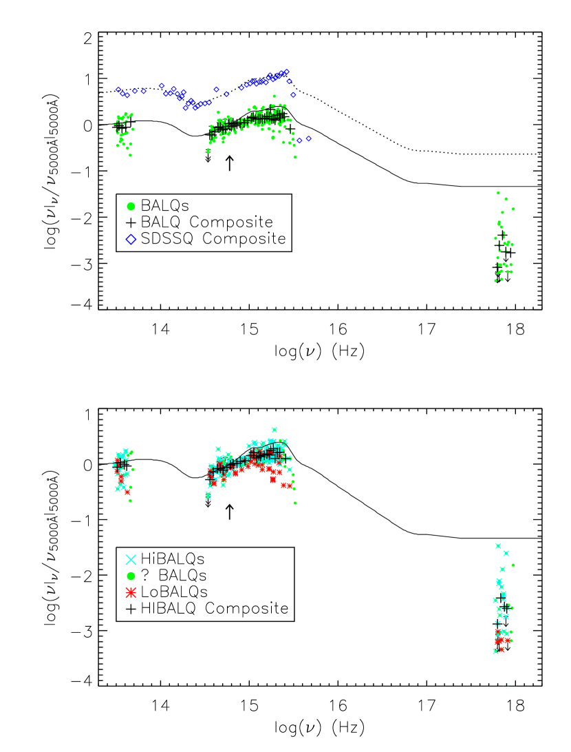
Figure 5.— Mid-infrared-to-X-ray BAL quasar composite SEDs. The algorithm for constructing the composite SEDs is described in §4.4. The data and the Richards et al. (2006) SDSS composite SED (black curve) have been normalized to $\nu$$l_{\rm 5000\AA}$. For reference, the 5000Å normalization point ($\log(\nu)=14.78$) is marked with an arrow, and 8 µm is at $\log(\nu)=13.57$. Top panel: All 38 BAL quasars (green filled circles) and their composite (black crosses); the SDSS comparison sample composite (blue diamonds) and its corresponding Richards et al. (2006) SED (dotted curve) are offset vertically for clarity. Bottom panel: The HiBAL quasar composite SED (black crosses) and the BAL quasar data delineated by BAL type: Hi (cyan $\times$), unknown (green filled circles), and Lo (red $\ast$).

References

- Avni & Tananbaum (1986) Avni, Y. & Tananbaum, H. 1986, ApJ, 305, 83
- Barvainis (1987) Barvainis, R. 1987, ApJ, 320, 537
- Becker et al. (2000) Becker, R. H., White, R. L., Gregg, M. D., Brotherton, M. S., Laurent-Muehleisen, S. A., & Arav, N. 2000, ApJ, 538, 72
- Brotherton et al. (2006) Brotherton, M. S., de Breuck, C., & Schaefer, J. J. 2006, MNRAS, L90
- Canalizo & Stockton (2001) Canalizo, G. & Stockton, A. 2001, ApJ, 555, 719
- Clavel et al. (2006) Clavel, J., Schartel, N., & Tomas, L. 2006, A&A, 439
- Condon et al. (1998) Condon, J. J., Cotton, W. D., Greisen, E. W., Yin, Q. F., Perley, R. A., Taylor, G. B., & Broderick, J. J. 1998, AJ, 115, 1693
- Cristiani & Vio (1990) Cristiani, S. & Vio, R. 1990, A&A, 227, 385
- Edelson & Malkan (1986) Edelson, R. A. & Malkan, M. A. 1986, ApJ, 308, 59
- Efstathiou et al. (2000) Efstathiou, A., Rowan-Robinson, M., & Siebenmorgen, R. 2000, MNRAS, 313, 734
- Elvis et al. (1994) Elvis, M., et al. 1994, ApJS, 95, 1
- Everett (2005) Everett, J. E. 2005, ApJ, 631, 689
- Fritz et al. (2006) Fritz, J., Franceschini, A., & Hatziminaoglou, E. 2006, MNRAS, 366, 767
- Gallagher et al. (2002) Gallagher, S. C., Brandt, W. N., Chartas, G., & Garmire, G. P. 2002, ApJ, 567, 37
- Gallagher et al. (2006) Gallagher, S. C., Brandt, W. N., Chartas, G., Priddey, R., Garmire, G. P., & Sambruna, R. M. 2006, ApJ, 644, 709
- Gallagher et al. (2007) Gallagher, S. C., Richards, G. T., Lacy, M., Hines, D. C., Elitzur, M., & Storrie-Lombardi, L. J. 2007, ApJ, in press, astro-ph/0702272
- Goodrich (1997) Goodrich, R. W. 1997, ApJ, 474, 606
- Granato et al. (2004) Granato, G. L., De Zotti, G., Silva, L., Bressan, . A., & Danese, L. 2004, ApJ, 600, 580
- Green & Mathur (1996) Green, P. J. & Mathur, S. 1996, ApJ, 462, 637
- Gregg et al. (2002) Gregg, M. D., Becker, R. H., White, R. L., Richards, G. T., Chaffee, F. H., & Fan, X. 2002, ApJ, 573, L85
- Haas et al. (2003) Haas, M., et al. 2003, A&A, 402, 87
- Hamann et al. (1993) Hamann, F., Korista, K. T., & Morris, S. L. 1993, ApJ, 415, 541
- Hewett & Foltz (2003) Hewett, P. C. & Foltz, C. B. 2003, AJ, 125, 1784
- Hewett et al. (1995) Hewett, P. C., Foltz, C. B., & Chaffee, F. H. 1995, AJ, 109, 1498
- Hewett et al. (2001) — 2001, AJ, 122, 518
- Hopkins et al. (2005) Hopkins, P. F., Hernquist, L., Martini, P., Cox, T. J., Robertson, B., Di Matteo, T., & Springel, V. 2005, ApJ, 625, L71
- Korista et al. (1993) Korista, K. T., Voit, G. M., Morris, S. L., & Weymann, R. J. 1993, ApJS, 88, 357
- Krolik & Voit (1998) Krolik, J. H. & Voit, G. M. 1998, ApJ, 497, L5
- La Valley et al. (1992) La Valley, M., Isobe, T., & Feigelson, E. 1992, in ASP Conf. Ser. 25: Astronomical Data Analysis Software and Systems I, eds. D. M. Worrall, C. Biemesderfer, & J. Barnes, vol. 1, 245
- Lamy & Hutsemékers (2004) Lamy, H. & Hutsemékers, D. 2004, A&A, 427, 107
- Lewis et al. (2003) Lewis, G. F., Chapman, S. C., & Kuncic, Z. 2003, ApJ, 596, L35
- Low et al. (1988) Low, F. J., Huchra, J. P., Kleinmann, S. G., & Cutri, R. M. 1988, ApJ, 327, L41
- Maddox & Hewett (2006) Maddox, N. & Hewett, P. C. 2006, MNRAS, 367, 717
- Murray et al. (1995) Murray, N., Chiang, J., Grossman, S. A., & Voit, G. M. 1995, ApJ, 451, 498
- Ogle et al. (1999) Ogle, P. M., Cohen, M. H., Miller, J. S., Tran, H. D., Goodrich, R. W., & Martel, A. R. 1999, ApJS, 125, 1
- Page et al. (2005) Page, K. L., Reeves, J. N., O’Brien, P. T., & Turner, M. J. L. 2005, MNRAS, 898
- Priddey et al. (2007) Priddey, R. S., Gallagher, S. C., Isaak, K. G., Sharp, R. G., McMahon, R. G., & Butner, H. M. 2007, MNRAS, 374, 867
- Priddey & McMahon (2001) Priddey, R. S. & McMahon, R. G. 2001, MNRAS, 324, L17
- Proga et al. (2000) Proga, D., Stone, J. M., & Kallman, T. R. 2000, ApJ, 543, 686
- Reichard et al. (2003a) Reichard, T. A., et al. 2003a, AJ, 125, 1711
- Reichard et al. (2003b) — 2003b, AJ, 126, 2594
- Richards et al. (2002) Richards, G. T., Vanden Berk, D. E., Reichard, T. A., Hall, P. B., Schneider, D. P., SubbaRao, M., Thakar, A. R., & York, D. G. 2002, AJ, 124, 1
- Richards et al. (2006) Richards, G. T., et al. 2006, ApJS, in press, (astro-ph/0601558)
- Rowan-Robinson (2000) Rowan-Robinson, M. 2000, MNRAS, 316, 885
- Sanders et al. (1988) Sanders, D. B., Soifer, B. T., Elias, J. H., Neugebauer, G., & Matthews, K. 1988, ApJ, 328, L35
- Scannapieco & Oh (2004) Scannapieco, E. & Oh, S. P. 2004, ApJ, 608, 62
- Schneider et al. (2005) Schneider, D. P., et al. 2005, AJ, 130, 367
- Schweitzer et al. (2006) Schweitzer, M., et al. 2006, ApJ, in press, (astro-ph/0606158)
- Skrutskie et al. (2006) Skrutskie, M. F., et al. 2006, AJ, 131, 1163
- Spergel et al. (2003) Spergel, D. N., et al. 2003, ApJS, 148, 175
- Spergel et al. (2007) — 2007, ApJ, in press, (astro-ph/0603449)
- Sprayberry & Foltz (1992) Sprayberry, D. & Foltz, C. B. 1992, ApJ, 390, 39
- Springel et al. (2005) Springel, V., Di Matteo, T., & Hernquist, L. 2005, MNRAS, 361, 776
- Steffen et al. (2006) Steffen, A. T., Strateva, I., Brandt, W. N., Alexander, D. M., Koekemoer, A. M., Lehmer, B. D., Schneider, D. P., & Vignali, C. 2006, AJ, 131, 2826
- Stocke et al. (1992) Stocke, J. T., Morris, S. L., Weymann, R. J., & Foltz, C. B. 1992, ApJ, 396, 487
- Strateva et al. (2005) Strateva, I. V., Brandt, W. N., Schneider, D. P., Vanden Berk, D. G., & Vignali, C. 2005, AJ, 130, 387
- Trump et al. (2006) Trump, J. R., et al. 2006, ApJS, 165, 1
- Vanden Berk et al. (2001) Vanden Berk, D. E., et al. 2001, AJ, 122, 549
- Weymann et al. (1991) Weymann, R. J., Morris, S. L., Foltz, C. B., & Hewett, P. C. 1991, ApJ, 373, 23
- White et al. (1997) White, R. L., Becker, R. H., Helfand, D. J., & Gregg, M. D. 1997, ApJ, 475, 479
- White et al. (1997) White, R. L., et al. 2000, ApJS, 126, 133
- Willott et al. (2003) Willott, C. J., Rawlings, S., & Grimes, J. A. 2003, ApJ, 598, 909
- York et al. (2000) York, D. G., et al. 2000, AJ, 120, 1579
- Zhou et al. (2006) Zhou, H., Wang, T., Wang, H., Wang, J., Yuan, W., & Lu, Y. 2006, ApJ, 639, 716