Radio-frequency discharges in Oxygen. Part 1: Modeling

Abstract

In this series of three papers we present results from a combined experimental and theoretical effort to quantitatively describe capacitively coupled radio-frequency discharges in oxygen. The particle-in-cell Monte-Carlo model on which the theoretical description is based will be described in the present paper. It treats space charge fields and transport processes on an equal footing with the most important plasma-chemical reactions. For given external voltage and pressure, the model determines the electric potential within the discharge and the distribution functions for electrons, negatively charged atomic oxygen, and positively charged molecular oxygen. Previously used scattering and reaction cross section data are critically assessed and in some cases modified. To validate our model, we compare the densities in the bulk of the discharge with experimental data and find good agreement, indicating that essential aspects of an oxygen discharge are captured.

I I. Introduction

Electro-negative gases, such as ${\rm SF_{6}}$, ${\rm Cl_{2}}$, ${\rm CF_{4}}$, and ${\rm O_{2}}$, play an important role in plasma-assisted materials processing. Most notably ${\rm O}_{2}$, either as the main feedstock gas or as an admixture to halogen- or silicon-based gases, is of vital importance for a large variety of etching and thin-film deposition techniques Tolliver (1984); Siejka and Perriere (1989); Carl et al. (1991); Kitajima et al. (1992); Kizling and Jaeras (1996); Nicolazo et al. (1998); Meichsner et al. (1998). The requirements on the controllability and predictability of these processes are so high that further advancement of this technology will depend on modeling tools which go beyond the macroscopic, fluid-type approximations, which, for instance, cannot reliably predict the velocity distributions of the species.

Although electro-negative gas discharges have been studied for a long time Seeliger (1949); Sabadil (1973); Edgley and von Engel (1980), with significant progress made during the last two decades Ferreira et al. (1988); Tsendin (1989); Lichtenberg et al. (1994); Franklin and Snell (1999), a complete quantitative description is still lacking, in particular, with respect to discharge profiles, structuring, and operation regimes Franklin (2001a, 2002). This is not surprising because the occurrence of negative ions leads to abrupt changes in the ion density (density fronts Kaganovich (2001)) which in most cases force the discharge to stratify into a central quasi-neutral ion-ion plasma and a peripheral electro-positive electron-ion plasma Edgley and von Engel (1980); Ferreira et al. (1988); Tsendin (1989); Lichtenberg et al. (1994); Franklin and Snell (1999, 2000); Lampe et al. (2004). The transition between the two is rather subtle. It can be, for instance, accompanied by a double layer (internal sheath Kouznetsov et al. (1999)). Electro-negative gas discharges are thus rather complex and the investigation of the spatio-temporal structure of the discharge as a function of external control parameters (current, voltage, frequency, pressure, and geometry) is a great theoretical Boeuf (1987); Shveigert (1991); Kaganovich (1995); Lee et al. (2006) and experimental Quandt et al. (1998); Ishikawa et al. (1998); Katsch et al. (2000); Berezhnoj et al. (2000); Kono (2002); Dittmann et al. challenge. In addition, electro-negative processing gases are reactive molecular gases, with internal degrees of freedom, which lead to a quite involved plasma chemistry.

Similar to the kinetic description of a mixture of reacting gases Boffi and Rossani (1990), the modeling of a gas discharge could be based on a coupled set of Boltzmann equations for the distribution functions of the species which need to be treated kinetically. This set has to be augmented by Maxwell’s equations, or parts of it, depending on how the discharge is electrically driven. Even for simple reactive gas discharges, with only two negatively and one positively charged species, this approach is not practical. More promising are methods which track representative samples of simulated particles subject to (non-reactive and reactive) collisions as well as electromagnetic fields, which are again determined from the relevant parts of Maxwell’s equations. Although these approaches are closely related to the direct simulation method successfully employed for the modeling of the flow of rarefied gases Bird (1969); Nanbu (1980); Bird (1994), in the context of gas discharges Nanbu (2000), it is more common to refer to them as particle-in-cell Monte Carlo collision (PIC-MCC) methods Vahedi and Surendra (1995); Kawamura et al. (2000); Tskhakaya and Kuhn (2002); Verboncoeur (2005), because without collisions the methods collapse to the PIC approach Birdsall and Langdon (1985); Hockney and Eastwood (1989) for the solution of the Vlasov problem.

This is the first paper in a series of three where we report the results of a combined experimental and theoretical study of the interplay between plasma-chemistry and electrodynamics in capacitively coupled radio-frequency (rf) discharges in oxygen. Oxygen is a weakly electro-negative gas whose plasma chemistry is strongly affected by vibrational, rotational and meta-stable states. Up to 75 reaction and scattering processes have been listed to potentially affect the properties of the discharge Kiehlbauch and Graves (2003). Not all of them can be equally important. The challenge is therefore to identify (via comparison between experiment and modeling) the subset of collisions responsible for the experimental findings under consideration.

In the present paper, we describe such a reduced model. It is tailor-made for the investigation of the charged species of the discharge, including the formation of ion density fronts, internal sheaths, and the resulting stratification of the discharge. We critically assess the cross sections used to characterize the selected collision channels and point out some inconsistencies in previously used cross section data. The validity of our model is verified by a comparison of calculated bulk densities with experimentally measured ones Katsch et al. (2000). The following two papers discuss, from the experimental Dittmann et al. and theoretical Matyash et al. point of view, respectively, the sheath region of the discharge focusing on the $844~{}nm$ double emission layer in front of the powered electrode and a comparison of experimental and simulated distribution functions for positive ions.

The next section describes the main features of our PIC-MCC implementation Takizuka and Abe (1977); Matyash (2003). It is an extension of a code, which was originally designed for the particle-based modeling of sheaths in magnetized plasmas Chodura (1982); Bergmann (1994), to the case of electrically driven discharges in reactive molecular gases. We focus, in particular, on the handling of collision processes, which deviates from the treatments usually employed in the plasma context Vahedi and Surendra (1995); Tskhakaya and Kuhn (2002); Verboncoeur (2005) and is closer to the simulation approaches used in rarefied gas dynamics Bird (1969, 1994). The collisions included in our model are discussed in Section III. Where necessary, we combine measured cross sections Phelps (1985); Gray and Rees (1972); Stebbings et al. (1963); Muschlitz (1960); Rapp and Briglia (1965); Tisone and Branscomb (1968); Peart et al. (1979); Vejby-Christensen et al. (1996); Walls and Dunn (1974); Padgett and Peart (1998); Comer and Schulz (1974a, b); Bailey and Mahadevan (1970) with model cross sections Olson (1972); Okada et al. (1978); Bardsley (1968); Akhmanov et al. (1982); Lieberman and Lichtenberg (2005) to characterize collisions and fix the free parameters through a comparison with experimental data. In Section IV we show that once the parameters are fixed, good agreement between simulation and experiment can be achieved in the bulk of the discharge. Section V summarizes the essentials of our model and concludes with a short outlook.

II II. Method of simulation

Figure 1: Schematic geometry of the rf discharges used in Refs. Katsch et al. (2000); Dittmann et al. . We use a planar, one-dimensional model to simulate the central axial part of the discharge (thick solid line).

We are only interested in the central axial part of the rf discharges described in Refs. Katsch et al. (2000); Dittmann et al. . Ignoring the electric asymmetry between the powered and grounded electrode, this part of the discharge can be simulated by the planar, one-dimensional model shown in figure 1. The planar model retains only one spatial coordinate $x$, with $0\leq x\leq L$, where $L$ is the distance between the electrodes, but it keeps the full three-dimensional velocity space for the particles (1d3v model). One of the electrodes is driven by the rf voltage $U(t)=U_{rf}\sin(2\pi f_{rf}t)$, with $f_{rf}=13.6~{}MHz$ and $U_{rf}$ ranging from $75~{}V$ to $800~{}V$, while the other is grounded. Both electrodes are assumed to be totally absorbing; secondary electron emission is neglected. To mimic the constant oxygen flow through the discharge chamber, we enforce in the simulation volume a constant oxygen pressure ranging from $10~{}Pa$ to $100~{}Pa$.

The simulation volume of the planar model is of course not well defined because the lateral “cross-section” A is a free parameter. This parameter actually controls the weight of the simulated particles, that is, the number of real particles represented by one simulated particle. We arbitrarily choose $A=\lambda_{De}^{2}$ with $\lambda_{De}$ the electron Debye length of a reference electron system (RES) which we use to initially set-up the length and time scales of the simulation (see below). The RES is specified by a density $n_{res}$ and a temperature $T_{res}$. Both have to be adjusted to the particular experimental conditions. For the experiments Katsch et al. (2000); Dittmann et al. , $n_{res}\approx 10^{8}~{}$–$~{}10^{9}~{}cm^{-3}$ and $k_{B}T_{res}~{}\approx~{}10~{}eV$, resulting in approximately $10^{5}$ simulated particles.

The complex plasma-chemistry of oxygen gives rise to a large number of non-reactive and reactive collisions Kiehlbauch and Graves (2003). In table 1 we show the ones with the largest cross sections. They are included in our model and will be discussed in detail in Section III. We treat only three species kinetically: electrons ($e$), negatively charged oxygen atoms ($O^{-}$), and positively charged oxygen molecules ($O_{2}^{+}$). Neutral particles appearing either as educts or products in table 1 are not explicitly simulated. Molecular oxygen in its ground state, $O_{2}$ (feedstock gas), is modelled as a reservoir characterized by a pressure $p$ and a temperature $T$. Whereas atomic oxygen, $O$, vibrationally excited oxygen molecules, $O_{2}(\nu)$, the Rydberg state of the molecular oxygen, $O_{2}({\rm Ryd})$, and the molecular meta-stables, $O_{2}(a^{1}\Delta_{g})$ and $O_{2}(a^{1}\Sigma_{g})$, are only indirectly accounted for in as far as their production results in an energy loss for electrons.

The meta-stable $O_{2}(a^{1}\Delta_{g})$ requires special attention because it also appears as an educt in the entrance channel for associative detachment (17). Its concentration is therefore important, and we should actually build-up the $O_{2}(a^{1}\Delta_{g})$ distribution function, that is, we should also simulate $O_{2}(a^{1}\Delta_{g})$ particles. In that case, however, not only their volume production process (11) but also their volume and surface loss processes should be included. This is beyond the one-dimensional model. To take associative detachment, which is known to be an important process Shibata et al. (1996); Katsch et al. (2000); Franklin (2001b); Belostotsky et al. (2005), nevertheless into account, we use instead a simple model with one free parameter, which can be interpreted as the $O_{2}(a^{1}\Delta_{g})$ to $O_{2}$ density ratio (see below).

The three-species PIC-MCC model describes the physics of an ${\rm O}_{2}$ discharge by tracing the spatio-temporal evolution of an ensemble of charged particles ($e$, ${\rm O}^{-}$, and ${\rm O}_{2}^{+}$). As usual, to track the velocities and positions of the simulated particles, the simulation domain $0\leq x\leq L$ and the time are discretized and free flights are decoupled from collisions (see figure 2). In order to have stable free flights of charged particles (in the mean electric field given by the Poisson equation), the spatial resolution $\Delta x$ has to be less then the electronic Debye length, $\lambda_{De}$, and the time step $\Delta t$ should resolve the electron plasma oscillation whose frequency is $\omega_{pe}$ Birdsall and Langdon (1985); Hockney and Eastwood (1989). Both $\lambda_{De}$ and $\omega_{pe}$ are set by the RES.

The time interval over which collisions and free flights are decoupled is of the order of the mean free time, which, in general, is much larger then the fundamental time step $\Delta t$ enforced by the electric field. We distinguish two groups of collisions, each of which characterized by an average mean free time. The first group of collisions, occurring on a time scale $\Delta t_{c,1}$ comprises all collisions of table 1 except Coulomb collisions between charged particles, which take place on a different time scale $\Delta t_{c,2}$.

Figure 2: Graphical representation of our implementation of the PIC-MCC scheme.

To build up a representative sample for the charged particles, we first sample the initial distribution functions for $e$, ${\rm O}^{-}$, and ${\rm O}_{2}^{+}$ and then repeat the following procedure Matyash (2003) (see figure 2):

• For $n_{1}=\Delta t_{c,1}/\Delta t$ time steps, the coordinates and velocities of all simulated particles are moved according to Newton’s equations of motion. The force acting on particles with charge $q_{i}$ is given by ${\bf F_{i}}=-q_{i}\nabla\Phi$ where $\Phi$ is the electric potential satisfying the Poisson equation with the boundary conditions specified above. Force interpolation and charge assignment are done within a linear interpolation scheme.

• After $n_{1}$ time steps, a representative sample of the first class of collisions is executed, with post-collision velocities stochastically determined in accordance with energy and momentum conservation, followed by free flights with $n_{1}-n_{2}$ time steps, where $n_{2}=\Delta t_{c,2}/\Delta t$, after which a representative random sample of Coulomb collisions is performed, again consistent with energy and momentum conservation.

After typically $10^{3}$ rf cycles quasi-stationarity with respect to the rf cycle is achieved, that is, within the statistical noise, macroscopic quantities, for instance, density and potential profiles, do not change anymore when averaged over a rf cycle.

Our treatment of collisions utilizes a number of concepts originally developed for the direct simulation Monte Carlo of rarefied gas flows Bird (1969, 1994). Since it differs from the handling of collisions in the standard PIC-MCC schemes, which is based on the null-collision method Vahedi and Surendra (1995), we give some more details. After a free flight is completed, we sort the simulated particles into cells (see figure 2). Simulated and feedstock gas particles located in one and the same cell (collisions are local) have then the opportunity to sequentially perform all possible types of collisions with each other. Simulated particles produced in the exit channel of a collision are readmitted for the next collision in the list. The ordering of particles into cells has to be repeated after each collision producing or annihilating simulated particles. Thus, as in the real system, simulated particles may perform more than one type of collision within the time interval over which the simulation decouples free flights and collisions.

The probability of a simulated particle $i$ to make a collision of type $j$ is given by

$$P_{j}^{(i)}=n_{j}\sigma_{j}u_{j}^{(i)}\tau_{j}~{}.$$ (1)

It depends on the density $n_{j}$ of the collision partners which act as the targets, the total cross section $\sigma_{j}$ for the collision, the relative velocity $u_{j}^{(i)}$ between particle $i$ and a particular collision partner, and the mean free time $\tau_{j}$. As can be seen in table 1, except for associative detachment (17), which we discuss in more detail in the next section, the three species model recruits collision partners either from the simulated particles or from the feedstock gas ${\rm O_{2}}$. In the first case, $n_{j}$ is the number of simulated particles of the respective type in the considered cell divided by the cell volume, whereas in the second case, $n_{j}=p/kT$, with $p$ the gas pressure and $T$ the room temperature. We do not calculate the mean free times $\tau_{j}$ for all the collisions listed in table 1. Instead, we set $\tau_{j}=\Delta t_{c,2}$ for Coulomb collisions (1) – (3) and $\tau_{j}=\Delta t_{c,1}$ for the remaining collisions (4) – (19).

In order to verify that our code treats collisions correctly, we performed various test runs and compared the results either with analytical results Matyash (2003) or with results obtained from the BIT1 code Tskhakaya and Kuhn (2002). The latter was also used to check discrepancies in the cross section data.

III III. Scattering and reaction channels

Table 1: Collisions included in our model

elastic scattering
(1) ${e+e\rightarrow e+e}$
(2) ${\rm O^{-}+O^{-}\rightarrow O^{-}+O^{-}}$
(3) ${\rm O_{2}^{+}+O_{2}^{+}\rightarrow O_{2}^{+}+O_{2}^{+}}$
(4) ${\rm e+O_{2}\rightarrow e+O_{2}}$
(5) ${\rm O^{-}+O_{2}\rightarrow O^{-}+O_{2}}$
(6) ${\rm O_{2}^{+}+O_{2}\rightarrow O_{2}+O_{2}^{+}}$	charge exchange
electron energy loss scattering
(7) ${\rm e+O_{2}\rightarrow e+O_{2}(\nu=1,...,4)}$	vibrational excitation
(8) ${\rm e+O_{2}\rightarrow e+O_{2}(Ryd)}$	Rydberg excitation
(9) ${\rm e+O_{2}\rightarrow e+O(3P)+O(3P)}$	dissociation (6.4 eV)
(10) ${\rm e+O_{2}\rightarrow e+O(3P)+O(1D)}$	dissociation (8.6 eV)
(11) ${\rm e+O_{2}\rightarrow e+O_{2}(a^{1}\Delta_{g})}$	meta-stable excitation
(12) ${\rm e+O_{2}\rightarrow e+O_{2}(b^{1}\Sigma_{g})}$	meta-stable excitation
electron $\&$ ion production $\&$ loss
(13) ${\rm e+O_{2}^{+}\rightarrow O+O}$	dissociative recombination
(14) ${\rm O^{-}+O_{2}^{+}\rightarrow O+O_{2}}$	neutralization
(15) ${\rm e+O_{2}\rightarrow O+O^{-}}$	dissociative attachment
(16) ${\rm O^{-}+O_{2}\rightarrow O+O_{2}+e}$	direct detachment
(17) ${\rm O^{-}+O_{2}(a^{1}\Delta_{g})\rightarrow O_{3}+e}$	associative detachment
(18) ${\rm e+O_{2}\rightarrow 2e+O_{2}^{+}}$	impact ionization
(19) ${\rm e+O^{-}\rightarrow O+2e}$	impact detachment

Collisions strongly influence the particle concentration and the energy balance in the discharge. For oxygen, an overwhelming number of elastic, inelastic, and reactive collisions is possible. Restricting, however, the description to a three species plasma ($e$, ${\rm O}^{-}$, and ${\rm O}_{2}^{+}$) many processes can be ignored and others can be treated approximately. In table 1 we show the collisions defining our three species model for an oxygen discharge, and classify them into three groups: elastic scattering, electron energy loss scattering, and electron and ion production and loss reactions. The respective cross sections for these processes are shown in figures 3 – 6 as a function of the relative energy of the two particles in the entrance channel of the respective process.

Our collection of cross sections is semi-empirical, combining measured data, which is usually available only in a finite energy range, with simple models for the low-energy asymptotic, which in most cases is not very well known from experiments. In general, the high-energy asymptotic has to be also determined from models, but it is less critical because the distribution functions usually decay sufficiently fast at high energies. If not stated otherwise, we extrapolated therefore the values of the cross sections for the largest energies shown in the plots to all energies above it. Some of the cross sections significantly deviate from the ones previously used Vahedi and Surendra (1995). Our simulations indicate, however, that the modifications are essential for obtaining bulk densities in accordance with experiments Katsch et al. (2000); Dittmann et al. .

III.1 A. Elastic scattering

Elastic collisions (1) – (6) are particle number conserving. Thus, when a collision takes place, only the post-collision velocities of the scattering partners have to be determined whereas the list of simulated particles remains unaltered.

The first three scattering processes (1) – (3) are intra-species Coulomb collisions. They are not very important for the experiments Katsch et al. (2000); Dittmann et al. we analyze in this series of papers. For other parameter regimes, however, the local ion density in an electro-negative gas discharge can be rather high Kaganovich (1995) and it cannot be ruled out that ion-ion Coulomb collisions affect, for instance, the width of these ion density peaks. Since the computational burden is moderate, we kept intra-species Coulomb scattering in all our simulations. If not stated otherwise, inter-species Coulomb collisions were however neglected.

For Coulomb collisions, we used a binary collision model Takizuka and Abe (1977) with a uniformly distributed azimuth angle $\phi$, and a Gaussian distribution for $\tan\chi/2$, where $\chi$ is the scattering angle. The second moment of the Gaussian distribution is given by Takizuka and Abe (1977)

$$\langle\tan^{2}{\frac{\chi}{2}}\rangle=\frac{q^{4}n\ln\Gamma}{8\pi\epsilon_{0}m^{2}u^{3}}t_{c,2}~{},$$ (2)

with $t_{c,2}$ the collision time for Coulomb scattering, $\ln\Gamma$ the Coulomb logarithm, $u$ the magnitude of the relative velocity in the center-of-mass frame, and $n$, $q$, $m$, and $\epsilon_{0}$ the local density, the charge, the reduced mass of the charged species under consideration, and the dielectric constant of the vacuum, respectively.

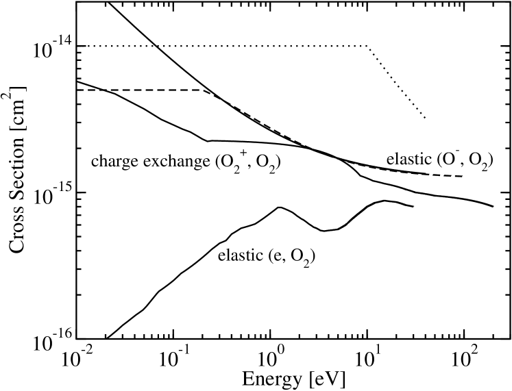
Figure 3: Cross sections for elastic scattering of electrons (4), ${\rm O}^{-}$ ions (5), and ${\rm O}_{2}^{+}$ ions (6) on oxygen molecules. The dashed line and the dotted line indicate, respectively, the cross section for elastic (${\rm O}^{-},{\rm O}_{2}$) scattering and the cross section for (${\rm O}^{+}_{2},{\rm O}_{2}$) charge exchange scattering used in Ref. Vahedi and Surendra (1995).

Figure 3 shows the cross sections for elastic scattering of electrons (4) and ${\rm O}^{-}$ ions (5) on ${\rm O}_{2}$ molecules together with the cross section for charge exchange scattering (6) of ${\rm O}_{2}^{+}$ ions on ${\rm O}_{2}$ molecules. Since little is known about the angle dependence of these processes, we assume the collisions to be isotropic, with a uniform distribution of the azimuth angle $\phi$ and a uniform distribution of $\cos{\chi}$, where $\chi$ is again the scattering angle.

The cross section for elastic scattering of electrons on ${\rm O}_{2}$ Phelps (1985) is the same as in Ref. Vahedi and Surendra (1995). The other two cross sections are different. For charge exchange scattering, we constructed the cross section as follows. Below $0.251~{}eV$ and above $8.5~{}eV$, we used empirical data for momentum transfer scattering Stebbings et al. (1963); Gray and Rees (1972), together with the expression

$$\sigma_{cx}(E)=\frac{1}{2}\sigma_{m}(E)~{},$$ (3)

where $\sigma_{m}$ and $\sigma_{cx}$ denote, respectively, the momentum and charge exchange cross section. For energies in between, we employed a linear interpolation. With this cross section, we could reproduce experimentally measured ${\rm O}_{2}^{+}$ velocity distribution functions very well Matyash et al. . With the charge exchange cross section given in Ref. Vahedi and Surendra (1995) (dotted line in figure 3), on the other hand, we could not obtain the correct distribution functions – neither with our PIC-MCC code nor with the BIT1 code Tskhakaya and Kuhn (2002), which we used in addition to exclude possible mistakes in our collision routines.

The cross section for elastic scattering of ${\rm O}^{-}$ on ${\rm O}_{2}$ originates from a model which assumes polarization scattering between the two, induced by a central potential $V(r)=-C/r^{n}$ with $n=3$. It is given by

$$\sigma_{e}(E)=\big{[}\frac{n\pi}{n-2}\big{(}\frac{n-2}{2}\cdot\frac{C}{E[eV]}\big{)}^{2/n}+\sigma_{0}\big{]}\cdot cm^{2}~{},$$ (4)

with $C=3.77\cdot 10^{-24}$ and $\sigma_{0}=1.2\cdot 10^{-15}$ Muschlitz (1960); Okada et al. (1978). Here, we added a constant shift $\sigma_{0}$ to match the cross section at high energies as given in Ref. Vahedi and Surendra (1995).

III.2 B. Electron energy loss scattering

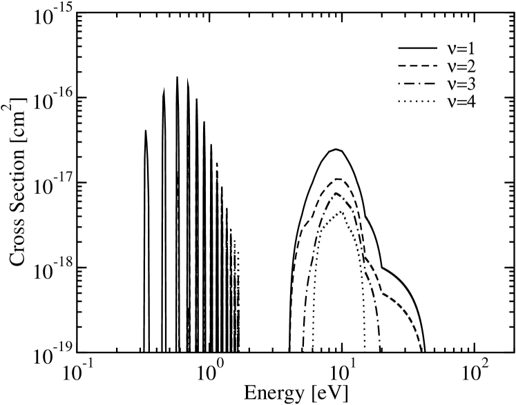
Figure 4: Cross sections for the $\nu=1,2,3,$ and $4$ vibrational excitation of ${\rm O}_{2}$ molecules (7).

Electron energy loss occurs due to inelastic collisions, (7) – (12), in which the oxygen molecule is either promoted into an excited state or dissociated into neutral fragments. In the three species model, where the spatio-temporal evolution of the neutral fragments and the excited oxygen molecules is not traced, we can treat this group of processes in the spirit of “test particle collisions” where the electron is the “test particle”, suffering momentum as well as energy transfer, and the ${\rm O}_{2}$ molecule is the “field particle” (with internal degrees of freedom). Drawing the field particles from a Maxwell distribution characterized by the gas temperature $T$ and the gas density $n=kT/p$, the same binary collision model can be used as for elastic scattering Takizuka and Abe (1977). The only difference is that now the magnitude of the post-collision relative velocity in the center-of-mass system is given by

$$u^{\prime}=\sqrt{u^{2}-\frac{2\delta E}{m_{\alpha\beta}}}~{},$$ (5)

where $u$ is the magnitude of the pre-collision relative velocity in the center-of-mass frame, $m_{\alpha\beta}$ is the reduced mass of the scattering partners, which, in general, have not the same mass, and $\delta E$ is the excitation energy of the process. Due to lack of angle-resolved scattering cross sections, we again assume the collisions to be isotropic.

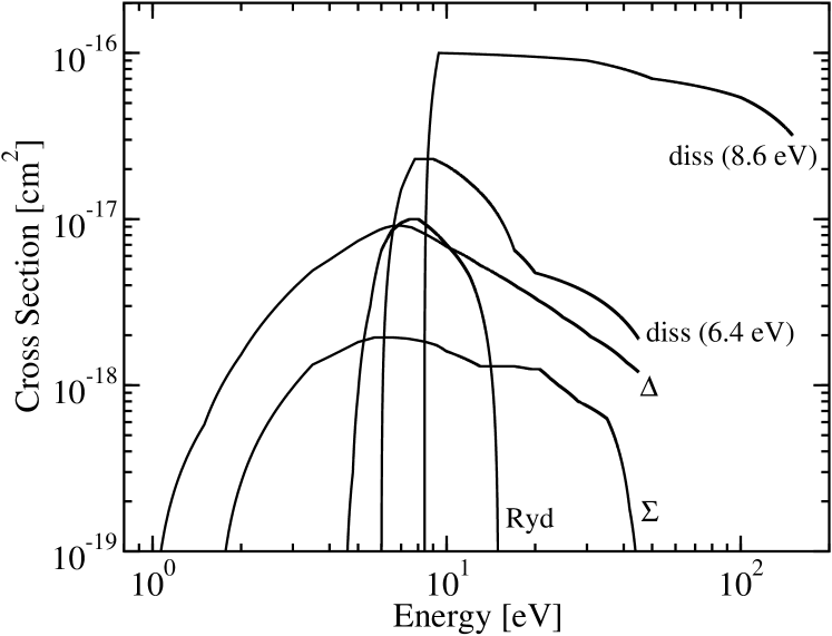
Figure 5: Cross sections for Rydberg excitation (8), $6.4~{}eV$ (9) and $8.6~{}eV$ (10) dissociative excitation, $\Delta$ excitation (11), and $\Sigma$ excitation (12) of ${\rm O}_{2}$ molecules.

The most important electron energy losses are due to vibrational and electronic excitation and impact dissociation of the oxygen molecule. The cross sections for these processes Phelps (1985) are the same as the ones used in Ref. Vahedi and Surendra (1995). For completeness, they are plotted in figures 4 and 5. We consider vibrational excitations with $\nu=1,2,3$, and $4$, excitation of the ${\rm O}_{2}$ Rydberg state, $PP$ and $PD$ dissociation, and the excitation of the meta-stable states ${\rm O_{2}(a^{1}\Delta_{g}})$ and ${\rm O_{2}(b^{1}\Sigma_{g}})$. In contrast to Ref. Vahedi and Surendra (1995), we ignore $DD$ dissociation, because, in the energy range of interest, its cross section is one order of magnitude smaller than for $PP$ and $PD$ dissociation, and rotational excitation which is almost elastic (small energy transfer) and thus dominated by the much more efficient elastic scattering of electrons on ${\rm O}_{2}$.

III.3 C. Electron and ion production and loss reactions

Electron and ion production and loss reactions (13) – (19) are inelastic collisions which change the number of charged particles. Therefore, the list of simulated particles has to be up-dated. All collisions obey conservation laws and are again assumed to be isotropic. The details of the modeling depend on the process.

The two recombination channels (13) and (14) result simply in the annihilation of the two oppositely charged particles which participate in the process. Binary collisions with one charged particle in the exit channel, such as dissociative attachment (15) and associative detachment (17), are treated within the modified binary collision model described in the previous subsection. Impact ionization (18) and impact detachment (19) are modelled as follows: First, an inelastic binary collision is performed, in which the parent electron looses the ionization (detachment) energy. Then, the post-collision ${\rm O}_{2}$ (${\rm O}^{-}$) particle is split into an electron and a ${\rm O}_{2}^{+}$ (${\rm O}$) particle. Finally, an elastic binary collision is applied to distribute energy among the two charged particles. Modeling three particle processes as a sequence of two binary collisions with a particle splitting in between guarantees energy and momentum conservation which is critical for the stability of simulations Matyash (2003). Although direct detachment (16) could be modelled in the same spirit, we adopted a simpler approach. From experiments Bailey and Mahadevan (1970) we know that the energy of the released electron is approximately one-tenth of the energy of the primary ${\rm O^{-}}$ ion. To obtain the energy distribution of the ejected electron we hardwired therefore this ratio in the collision routine for direct detachment.

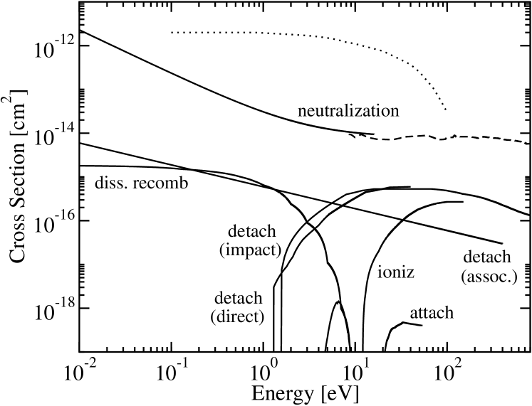
Figure 6: Cross sections for dissociative recombination (13), neutralization (14), dissociative attachment (15), direct detachment (16), associative detachment (17), impact ionization (18), and impact detachment (19). The dashed line indicates the experimentally determined high-energy asymptotic of the neutralization cross section and the dotted line is the cross section for neutralization used in Ref. Vahedi and Surendra (1995).

The cross sections for electron and ion production and loss reactions are shown in figure 6. For impact ionization Phelps (1985), dissociative attachment Rapp and Briglia (1965), and impact detachment Tisone and Branscomb (1968); Peart et al. (1979); Vejby-Christensen et al. (1996) we used empirical cross sections throughout, putting, in the case of impact detachment a higher confidence level to more recent data Vejby-Christensen et al. (1996), whereas for dissociative recombination, ion-ion neutralization, and detachment on neutrals we combined empirical data with analytical models.

First, we discuss dissociative recombination (13). For this process we used an effective cross section,

$$\sigma_{\rm dr}(E)=B\cdot\sigma_{0}(E)~{},$$ (6)

where $\sigma_{0}$ is the cross section for non-resonant dissociative recombination Bardsley (1968) and $B=3$ is a scaling factor, which is used to fit experimental data Walls and Dunn (1974). A comparison of the effective cross section with a calculated cross section Akhmanov et al. (1982) shows that $B$ can be also considered as a simple device to approximately take the effect of resonant dissociative recombination channels into account which originate from vibrationally excited states of $O_{2}^{+}$ Akhmanov et al. (1982).

For ion-ion neutralization (14), we constructed a cross section from a two-channel Landau-Zener model Olson (1972), with one free parameter, which we adjusted to obtain the correct high-energy asymptotic of the cross section Padgett and Peart (1998). Ion-ion neutralization occurs because the adiabatic energy of the $({\rm O^{-}},{\rm O}_{2}^{+})$ configuration decreases when the ions approach each other. At a certain distance $R_{x}$, the energy of the $({\rm O^{-}},{\rm O}_{2}^{+})$ configuration falls below the energy of the $({\rm O},{\rm O}_{2})$ configuration Lieberman and Lichtenberg (2005). The Landau-Zener theory estimates the probability for switching from one configuration to the other at the distance $R_{x}$ and leads to a cross section,

$$\sigma_{r}(E)=4\pi R_{x}^{2}\big{(}1+\frac{1}{R_{x}E}\big{)}~{},$$ (7)

which approaches a constant $C=4\pi R_{x}^{2}$ for $ER_{x}\gg 1$. Fitting $C$ and thus $R_{x}$ to empirical data at high energies Padgett and Peart (1998), we obtain

$$\sigma_{r}(E)=0.8\cdot\big{(}1+\frac{2.85}{E[eV]}\big{)}\cdot 10^{-14}\cdot cm^{2}~{}.$$ (8)

This cross section deviates dramatically from the one used in Ref. Vahedi and Surendra (1995) (dotted line in figure 6).

The most severe modification we made was for detachment of ${\rm O}^{-}$ on neutrals. It takes place through direct detachment (16), resulting in an atomic oxygen, an oxygen molecule and an electron, and through associative detachment (17), which leads to an ${\rm O}_{3}$ molecule and an electron. The latter is rather surprising because there is no evidence for it in beam experiments (where only direct detachment is observed Comer and Schulz (1974a, b)). Yet, experimental studies of ${\rm O}_{2}$ discharges Katsch et al. (2000); Belostotsky et al. (2005) (as well as general theoretical considerations Franklin (2002); Shibata et al. (1996); Franklin (2001b)) strongly suggest that associative detachment is possible in an oxygen discharge because of the presence of meta-stable ${\rm O}_{2}(a^{1}\Delta_{g})$. In contrast to direct detachment, which has a threshold around $1.3~{}eV$ Comer and Schulz (1974a) (see figure 6), associative detachment has usually no threshold. Thus, it may be a rather important loss channel for cold ${\rm O}^{-}$ ions.

Since we could not find an empirical cross section for associative detachment, we employed a model, which describes the detachment (electron loss) as the “inverse” of a classical Langevin-type electron capture into an attractive auto-detaching state of ${\rm O_{3}^{-}}$. Assuming the polarizability for ${\rm O}_{2}(a^{1}\Delta_{g})$ to be the same as for ${\rm O}_{2}$, the cross section is then given by Lieberman and Lichtenberg (2005)

$$\sigma^{\Delta}_{ad}(E)=5.96\cdot\frac{10^{-16}\cdot cm^{2}}{\sqrt{E[eV]}}~{}.$$ (9)

As can be seen in figure 6, associate detachment is already the dominant detachment process for energies below $\approx 6~{}eV$.

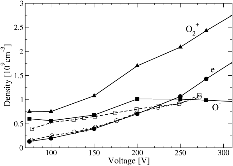
Figure 7: Voltage dependence of the quasi-stationary, cycle-averaged electron and ion densities at $x=L/2$ (bulk densities) for a discharge with $L=2.5~{}cm$, $p=13.8~{}Pa$, and $f_{rf}=13.6~{}MHz$. Filled and open symbols denote, respectively, results of the simulation and experimentally measured densities Katsch et al. (2000). Solid and dashed lines guide the eye.

From the cross section alone, of course, we cannot determine the probability $P_{ad}$ for associative detachment. We also need the density of ${\rm O_{2}(a^{1}\Delta_{g})}$, which is unknown in the three species model. However, it should be of the order of the ${\rm O}_{2}$ density. Therefore, we write $n_{\Delta}=C\cdot n_{{\rm O}_{2}}$, with $C<1$, and obtain $P_{ad}=u\cdot\sigma_{ad}\cdot(C\cdot n_{{\rm O}_{2}})\cdot t_{c,1}$, where $C$ is a fit parameter which can be adjusted to experiments.

IV IV. Comparison with experiment

The plasma model described in the previous sections contains three parameters: $\sigma_{0}$, $B$, and $C$. The first two we fixed by a direct comparison of the model cross section with the measured cross section. The parameter $C$, in contrast, cannot be determined in this way, because it is not linked to a cross section. It denotes instead the fraction of ${\rm O}_{2}$ molecules in the meta-stable ${\rm O_{2}(a^{1}\Delta_{g})}$ state which in turn depends on the particular set-up of the discharge. We consider therefore $C$ as a free parameter which can be adjusted to the discharge to be modelled.

To validate our model we focus now on the oxygen discharge described in Ref. Katsch et al. (2000). In order to determine $C$, we simulated the discharge for $p=13.8~{}Pa$, $U_{rf}=250~{}V$, and $f_{rf}=13.6~{}MHz$, and tuned $C$ to reproduce the quasi-stationary, cycle-averaged negative and positive ion densities at $x=L/2$ (bulk densities); the bulk electron density matches then also because of quasi-neutrality in the bulk of the discharge. We obtained $C\approx 1/6$, implying that roughly one sixth of the ${\rm O}_{2}$ molecules is in the meta-stable state.

In figure 7 we plot the bulk ion and electron densities for $p=13.8~{}Pa$ over a wide voltage range, using however for all voltages $C\approx 1/6$, the value determined for $U_{rf}=250~{}V$. As can be seen, the agreement between simulation and experimental data Katsch et al. (2000) is rather good, indicating that our model captures the essential processes in the bulk of an oxygen discharge.

The precise value of $C$ should not be taken too serious because it is based on a rather crude model for associative detachment. More important is that without this process ($C=0$), the simulation could not reproduce the measured densities. This can be seen in figure 8, where we plot the quasi-stationary, cycle-averaged density profiles without (thin lines) and with associative detachment (thick lines) taken into account. (For these runs, we also included inter-species Coulomb collisions but the profiles without it are basically the same.) Neglecting associative detachment, the bulk ion densities turned out to be almost one order of magnitude too high. Remarkably, without associative detachment, the density profiles have the parabolic shape expected from ambipolar drift-diffusion models Edgley and von Engel (1980); Ferreira et al. (1988); Tsendin (1989); Lichtenberg et al. (1994); Franklin and Snell (1999, 2000); Lampe et al. (2004).

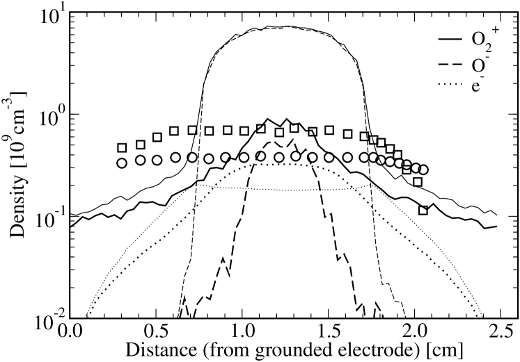
Figure 8: Quasi-stationary, cycle-averaged electron and ion density profiles for $U=150~{}V$ without (thin lines) and with (thick lines) associative detachment taken into account; $p$, $L$, and $f_{rf}$ are the same as in figure 7. Open circles and open squares denote, respectively, the measured electron and ${\rm O}^{-}$ density profiles Katsch et al. (2000). Note, the runs producing the shown data included inter-species Coulomb scattering.

To understand why associative detachment is so crucial for modeling the discharge of Ref. Katsch et al. (2000), we plot in figure 9 for $p=13.8~{}Pa$ and $U_{rf}=150~{}V$ the (marginal) velocity distribution function for negative ions, $f_{-}(E,x)$ with $E={\rm sign}(v_{x})v_{x}^{2}/2M_{-}$. Clearly, the majority of ${\rm O}^{-}$ ions is cold; the distribution function spreads out only in the region where the bulk plasma merges with the peripheral plasma at $x\approx 0.8~{}cm$. Thus, loss processes whose cross sections are large for small energies (see figure 6), that is, ion-ion neutralization and associative detachment, will be very efficient. Direct detachment, on the other hand, whose cross section has a threshold, will be suppressed. At low energies, both ion-ion neutralization and associative detachment have cross sections which increase with decreasing energy. Which process dominates depends therefore also on the collision probability $P$. For ion-ion neutralization $P$ is proportional to the ${\rm O}_{2}^{+}$ density while for associative detachment it is proportional to the ${\rm O_{2}(a^{1}\Delta_{g})}$ density. Since for the discharge of Ref. Katsch et al. (2000), the ${\rm O}_{2}^{+}$ density is much smaller than the ${\rm O_{2}(a^{1}\Delta_{g})}$ density, which we estimated to be $1/6$ of the ${\rm O}_{2}$ density, associative detachment has to be the main loss process for negative ions in this experiment.

Figure 9: Quasi-stationary, cycle-averaged negative ion velocity distribution function $f_{-}(E,x)$ with $E={\rm sign}(v_{x})v_{x}^{2}/2M_{-}$ for $U_{rf}=150~{}V$; $p$, $L$, and $f_{rf}$ as in figure 7.

Additional support for this claim comes from the weak voltage dependence of the ${\rm O}^{-}$ density between $75~{}V$ and $300~{}V$ indicating that both ${\rm O}^{-}$ production and ${\rm O}^{-}$ loss are in this voltage range rather insensitive to voltage changes. We will now show that this strongly suggests that associative detachment is the main loss process for ${\rm O}^{-}$ ions. First, we conclude from figure 10, which shows the attachment cross section (in arbitrary units) together with bulk electron velocity distribution functions for different voltages, that the energy range between $4~{}eV$ and $15~{}eV$ will be the most important one for the attachment process; for energies below $4~{}eV$ the production is zero because the cross section is zero while for energies above $15~{}eV$ the number of electrons available for attachment is too low. We also see that in the voltage range of interest, the electron velocity distribution function does not change much in this energy range. Thus, the production process is almost voltage-independent and the observed near constancy of the ${\rm O}^{-}$ density has to be taken as a signature of the loss process. As already mentioned, direct detachment can be ruled out. Ion-ion neutralization, on the other hand, would lead for $E\ll 1.4~{}eV$, that is, in the relevant energy range, to an energy-resolved rate coefficient $K_{r}(E)\sim\sqrt{E}\cdot\sigma_{r}(E)\sim 1/\sqrt{E}$ which strongly increases with decreasing energy. Thus, even small, voltage-induced changes of the energy of negative ions would suffice to lead to noticeable modifications of the loss rate. What remains is associative detachment. The energy-resolved rate coefficient for this process is $K_{ad}^{\Delta}(E)\sim\sqrt{E}\cdot\sigma_{ad}^{\Delta}(E)\sim const$. At the same time, the distribution function for ${\rm O^{-}}$ ions does not change much between $75~{}V$ to $300~{}V$. Thus, the loss rate due to associative detachment is nearly independent of voltage. Together with the voltage independence of dissociative attachment, this leads to the observed constancy of the ${\rm O^{-}}$ density.

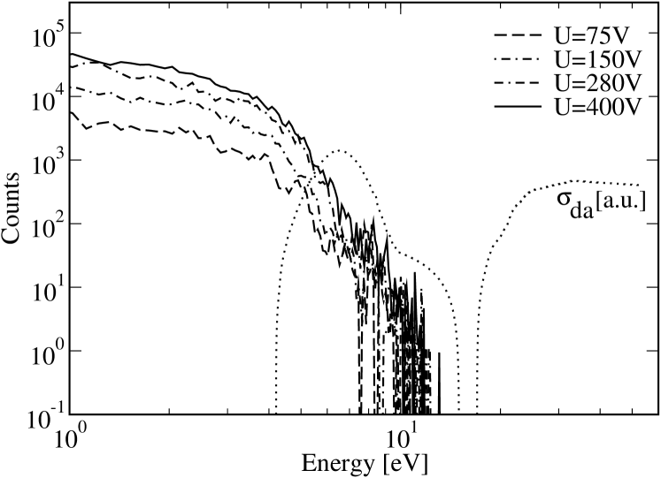
Figure 10: Quasi-stationary, cycle-averaged electron velocity distribution function $f_{e}(E,x)$ with $E=v^{2}/2m_{e}$ and $x=L/2$ for $U_{rf}=75~{}V,150~{}V,280~{}V$, and $300~{}V$; $p$, $L$, and $f_{rf}$ as in figure 7. The dotted line indicates the cross section for dissociative attachment (15) in arbitrary units.

Our simulation reproduces the absolute values of bulk densities fairly well. The (axial) density profiles of the simulation decay however too fast compared to the experimental ones (open symbols in figure 8). We attribute this to the fact that the simulations assume a constant ${\rm O}_{2}(a^{1}\Delta_{g})$ density, whereas, in reality, there should be a density profile, because of the interplay of volume and surface loss and generation processes for ${\rm O}_{2}(a^{1}\Delta_{g})$ molecules. In particular surface losses, that is, the decay of ${\rm O}_{2}(a^{1}\Delta_{g})$ molecules when they hit the boundary of the discharge should play an important role because they lead to a depletion of ${\rm O}_{2}(a^{1}\Delta_{g})$ molecules in the vicinity of the electrodes and thus to a reduction of associative detachment. A detailed investigation of the “drag” the ${\rm O}_{2}(a^{1}\Delta_{g})$ density is expected to exert on the ${\rm O^{-}}$ density is however beyond the scope of the present paper.

V V. Conclusions

We presented a planar, one-dimensional PIC-MCC model for a capacitively coupled rf discharge in oxygen which is capable to quantitatively describe experiments. Its main features are: (i) Only electrons, ${\rm O}^{-}$ ions, and ${\rm O}_{2}^{+}$ ions are treated kinetically. (ii) Neutral particles are only incorporated in as far as they affect the particle and energy balance of simulated charged particles. (iii) A direct simulation Monte Carlo model for collisions has been used, with two groups of collisions, which differ in the collision times.

The elementary processes of our three species model are shown in table 1. We took the processes with the largest cross sections into account. When possible, we implemented empirical cross sections. In some cases, however, we combined them with analytical model cross sections to obtain the correct low-energy asymptotic. In particular, we used a polarization-type scattering model for elastic $({\rm O}^{-},{\rm O}_{2})$ scattering, a Landau-Zener-type model for $({\rm O}^{-},{\rm O}_{2}^{+})$ neutralization, and an inverse classical, Langevin-type capturing model for ${\rm O}_{2}(a^{1}\Delta_{g})$-induced associative detachment. To describe associative detachment due to ${\rm O}_{2}(a^{1}\Delta_{g})$ without explicitly calculating the ${\rm O}_{2}(a^{1}\Delta_{g})$ density, we furthermore introduced a parameter $C$, which should be fitted to the particular oxygen discharge under consideration and could be interpreted as the fraction of ${\rm O}_{2}$ molecules in the meta-stable ${\rm O}_{2}(a^{1}\Delta_{g})$ state.

As a first application of our model, we simulated the discharge of Ref. Katsch et al. (2000). After we adjusted the parameter $C$ to reproduce the bulk ion densities for $p=13.8~{}Pa$ and $U_{rf}=250~{}V$, we also obtained the correct bulk densities for other voltages. The parameter $C\approx 1/6$, that is, approximately one sixth of the oxygen molecules are in the meta-stable state. We also pointed out that the weak voltage dependence of the bulk densities for fixed pressure indicates that ${\rm O}^{-}$ losses due to associative detachment dominate the ones due to ion-ion neutralization.

Although we could reasonably well describe electron and ion densities in the bulk, the (axial) ion density profiles of the simulation are too narrow compared to the experimental ones. Most probably this is because we assumed a constant ${\rm O}_{2}(a^{1}\Delta_{g})$ density. In reality, however, ${\rm O}_{2}(a^{1}\Delta_{g})$ molecules decay when they hit the boundary of the discharge. The ${\rm O}_{2}(a^{1}\Delta_{g})$ density should therefore decrease in the vicinity of the electrodes and with it associative detachment. To take this effect into account requires however a model which not only treats electrons, ${\rm O}^{-}$ ions, and ${\rm O}_{2}^{+}$ ions kinetically, but also ${\rm O}_{2}(a^{1}\Delta_{g})$ molecules.

Our concern in the present paper, which is the first in a series of three, was the calibration and validation of a three species model for capacitively coupled rf discharges in oxygen. For that purpose, we used published experimental data for the bulk of the discharge Katsch et al. (2000). The following paper Dittmann et al. describes the results of an experimental investigation of the sheath region of such a discharge, focusing, among others, on the spatial and temporal evolution of the $844~{}nm$ double emission layer in front of the powered electrode. In the third paper Matyash et al. , finally, we will use the three species model to simulate the sheath region. Besides a comparison of simulated with measured distribution functions for positive ions, we will also present a model for the $844~{}nm$ double emission layer. The three species model, including its approximate treatment of associative detachment, is sufficient for that purpose, because negative ions are negligible in the region from which the emission originates. Negative ions are only needed for the overall charge balance of the discharge. Their density profile per se is not crucial for the explanation of the $844~{}nm$ double emission layer as long as it features a vanishingly small density in front of the electrode. This is already accomplished by the three species model.