A cold metal-poor cloud traced by a weak Mg ii absorption at $z\simeq 0.45$

Abstract

Aims. We present the observations of a weak Mg ii absorption system detected at $z\sim 0.452$ in the UVES high-resolution spectrum of the QSO HE0001-2340. The weaker of the two Mg ii components forming the system shows associated absorptions due to Si i, Ca i, and Fe i observed for the first time in a QSO spectrum. We investigate the nature of this absorber by comparing its properties with those of different classes of absorbers and reproducing its ionization conditions with photoionization models.

Methods. We measured column densities of Mg i, Mg ii, Si i, Ca i, Ca ii, Mn ii, Fe i, and Fe ii with Voigt profile fitting. Although most of the observed velocity profiles are not resolved in the UVES spectrum, a curve of growth analysis excluded a significant underestimation of the column densities, in particular for the Fe ii and Mg ii multiplets. We compared our measurements with a sample of 28 weak Mg ii systems detected in the interval $0.4<z<1.4$ in the 18 UVES spectra of the ESO Large Programme, plus 24 weak Mg ii systems in the same redshift range taken from the literature. Then, we performed a comparison with 11 damped systems for which ionic column densities were measured component by component and with 44 Galactic lines of sight with measured Ca i, Ca ii and Fe i. We also ran a grid of photoionization models with Cloudy to reproduce the observed Mg i/Mg ii, Ca i/Ca ii, and Fe i/Fe ii column density ratios for the studied system.

Results. The observed absorber belongs to the class of weak Mg ii systems on the basis of its equivalent width, however the relative strength of commonly observed transitions deviates significantly from those of the above mentioned absorbers. A rough estimate of the probability of crossing such a system with a QSO line of sight is $P\sim 0.03$. The presence of rare neutral transitions suggests that the cloud is shielded by a large amount of neutral hydrogen. A detailed comparison of the observed column densities with the average properties of damped Lyman-$\alpha$ systems and local interstellar cold clouds shows, in particular, deficient Mg ii/Mg i and Ca ii/Ca i ratios in our cloud. The results of photoionization models indicate that the cloud could be ionized by the UV background. However, a simple model of a single cloud with uniform density cannot reproduce the observed ionic abundance ratios, suggesting a more complex density structure for the absorber. Supposing that ionization corrections are negligible, the most puzzling result is the underabundance of magnesium with respect to iron which is hard to explain both with nucleosynthesis and with differential dust depletion.

1 Introduction

Metal absorption systems observed in the spectra of high-redshift QSOs are extremely useful for studying the nature and evolution of star formation and gas chemical pollution through the cosmic ages.

Damped Lyman-$\alpha$ systems (DLA) are the highest neutral-hydrogen column density absorbers observed in QSO spectra ($N($H i$)\geq 2\times 10^{20}$ cm^-2). Such an amount of neutral gas is usually measured in local spiral discs, and it ensures an extremely precise determination of the chemical abundances due to the negligible ionization corrections (Vladilo 2001). Cold neutral clouds could also be the precursors of molecular clouds, the birthplace of stars. Indeed, molecular hydrogen has been observed in 13-20 percent of the DLA (Srianand et al. 2005), and DLA at $z\sim 3.0-4.5$ contain enough mass in neutral gas to account for a significant fraction of the visible stellar mass in modern galaxies (e.g. Storrie-Lombardi & Wolfe 2000).

DLA are selected mainly in the optical by looking for absorption features with equivalent width (EW) exceeding 5 Å in normalised QSO spectra (Prochaska et al. 2005, and references therein). At redshifts $z\la 1.6$, the Lyman-$\alpha$ line falls in the UV, requiring QSO observations from space; furthermore, at low z the interception probability per unit redshift is reduced. An efficient technique for collecting large samples of low-redshift DLA is to pre-select lines of sight showing Mg ii absorptions and then do the follow-up spectroscopy in the UV (Rao et al. 1995). The most recent observations by Rao et al. (2006) show that the fraction of DLA in a Mg ii sample increases with the Mg ii rest EW above a threshold value of $W_{o}^{\lambda 2796}=0.6$ Å. On the other hand, there is no correlation between $W_{o}^{\lambda 2796}$ and $N($H i$)$. The reasonable explanation given by Rao and collaborators is that the largest EW systems arise in clouds bounded in galaxy-sized potentials. A DLA system is observed if at least one of the clouds along the line of sight is cold (less than 100 K) and has a small velocity dispersion (a few km s^-1), so the larger the number of clouds along the sightline, the higher the probability of encountering a DLA system. Only rarely would a sightline intersect a single cloud resulting in small $W_{o}^{\lambda 2796}$ and large $N($H i$)$.

In this work, we present the discovery of a peculiar absorption system identified by a weak Mg ii doublet at $z\simeq 0.452$ along the line of sight to the bright QSO HE0001-2340. We compare its properties with those of weak Mg ii, DLA systems and with local diffuse clouds. We claim that we have detected a first example of a cold intergalactic cloud and discuss the implication of this finding. The structure of the paper is the following: Sect. 2 briefly presents the observational data and the reduction process; in Sect. 3 we report the results of the fit of the lines and the comparison of the obtained column densities and EWs with 3 samples of absorbers, each one presenting some characteristic in common with our system. In Sect. 4 we report the results from a grid of photoionization models run with Cloudy and we infer a physical model for the cloud. Finally, Sect. 5 is dedicated to the concluding remarks.

2 Observations and data reduction

The QSO HE0001-2340 ($z_{\rm em}$ $=2.267$) was observed with UVES (Dekker et al. 2000) at the ESO VLT in the context of the ESO Large Programme ‘The cosmic evolution of the IGM’ (Bergeron et al. 2004) at a resolution of $R\simeq 45000$ and signal-to-noise ratio $S/N\simeq 60-100$ per pixel. The wavelength range goes from 3100 to 10000 Å, except for the intervals $\sim 5760-5830$ and $8515-8660$ Å where the signal is absent due to the gap between the two CCDs forming the red mosaic.

The observations were reduced with the UVES pipeline (Ballester et al. 2000) in the context of the ESO MIDAS data reduction package, applying the optimal extraction methods and following the pipeline reduction step by step. Wavelengths were corrected to vacuum-heliocentric values, and individual 1D spectra were combined using a sliding window and weighting the signal by the total errors in each pixel.

The continuum level was determined by manually selecting regions of the spectrum free of evident absorptions, which were successively fitted with a 3rd-degree spline polynomial. Finally the spectrum was divided by this continuum, leaving only the information relative to absorption features.

3 Analysis

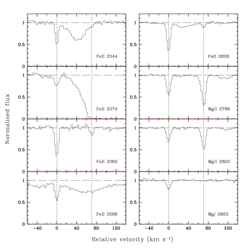
Figure 1: Transitions of Fe ii, Mg ii, and Mg i for the two velocity components of the discussed system. Velocity in the x axes is centered at the component which is discussed in the text ($z\simeq 0.4521$).

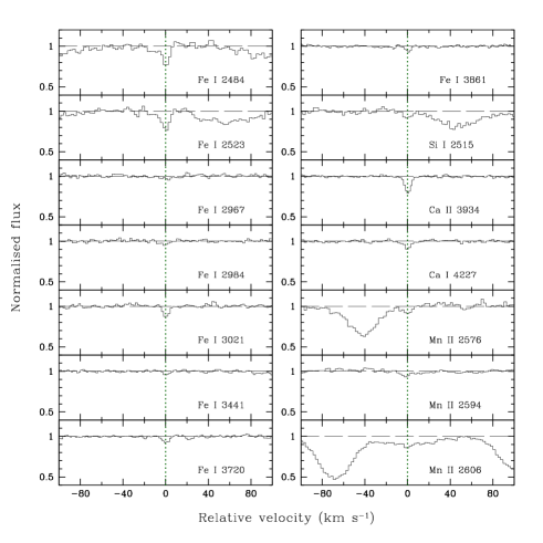
Figure 2: Other ionic transitions associated with the peculiar velocity component at $z\simeq 0.4521$. Fe i, Si i and Ca i were observed for the first time in a QSO absorption system.

In the process of detecting the metal lines contaminating the Lyman-$\alpha$ forest, we have identified an Mg ii doublet at $z\sim 0.452$ with the associated Fe ii absorption, composed of two extremely narrow components (see Fig. 1).

Surprisingly, at the redshift of the weaker Mg ii component, $z\simeq 0.45206$, we identified some ionic transitions generally observed in stronger Mg ii and DLA systems: Mg i $\lambda\,2852$, the triplet of Mn ii at $\sim 2600$ and Ca ii $\lambda\,3934$ Å (the other line of the doublet and the Na i doublet fall in the gap of the red CCDs). Even more exceptional is the detection of Ca i $\lambda\,4227$, Si i $\lambda\,2515$ Å, and several transitions due to Fe i. Those absorption lines are also weak in the local interstellar medium, and this is the first time that they are detected associated with a QSO absorber. All the detected absorption lines are shown in Figs. 1 and 2.

Voigt profiles were fitted to the observed absorption lines using the context Lyman (Fontana & Ballester 1995) of the ESO MIDAS package. The velocity profiles of the stronger transitions, Mg ii and Fe ii $\lambda\,2382$, 2600 Å, do not show any sign of blending, and their Doppler parameters are comparable to those found from the analysis of Mg ii and Fe ii absorption systems in very high resolution QSO spectra ($R\sim 120000$, Narayanan et al. 2006; Chand et al. 2006). The coincidence in redshift between different ions is of the order of 1 km s^-1 suggesting that neutral and singly ionized elements occupy the same region. The resulting Doppler parameters are all below $\sim 4$ km s^-1, even below 1 km s^-1 in the case of Fe i, implying that those lines are not resolved at the resolution of our spectrum (FWHM $\sim 6.7$ km s^-1). As a consequence, we could underestimate the column densities of the stronger transitions, if they are saturated.

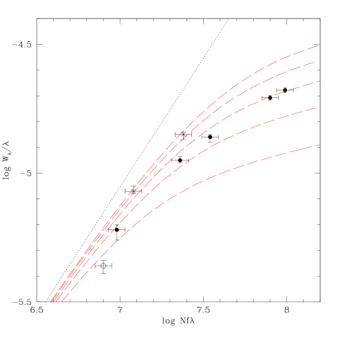
Figure 3: Data points obtained from the Voigt fit of Fe ii observed transitions (solid dots), the Mg ii doublet (crosses) and the line Ca ii $\lambda\,3934$ Å (open dot) compared with the theoretical curve of growths computed for $b=3,2.5,2,1.5,1$ km s^-1 (dashed lines from top to bottom). The dotted line represent the linear region of the curve of growth

In order to cross-check the results of our Voigt fit, a curve of growth analysis has been performed with the multiplet of Fe ii and the Mg ii doublet using EWs and column densities determined with MIDAS and comparing them with theoretical curve of growths at different Doppler parameters.

It is clear from Fig. 3 that the computed column densities are not significantly underestimated. On the contrary, they agree satisfactorily with the curve of growths with Doppler parameters between $\sim 1.5$ and 3 km s^-1. We also plot the result for Ca ii $\lambda\,3934$ Å, which is, however, more uncertain since we do not observe the other line of the doublet.

Table 1: Fit of the observed transitions and limits on the rest EWs for some transitions commonly observed in the cold interstellar medium.

Transition	$W_{\lambda}$	$\log N$	$b$
	mÅ	cm-2	km s-1
Mg ii $\lambda\,2796$	$39\pm 2$	$12.15\pm 0.03$	$2.6\pm 0.1$
Mg ii $\lambda\,2803$	$24\pm 2$	$12.15\pm 0.03$	$2.6\pm 0.1$
Mg i  $\lambda\,2852$	$18\pm 2$	$11.19\pm 0.02$	$2.9\pm 0.4$
Si i   $\lambda\,2515$	$8\pm 3$	$11.84\pm 0.05$	$3.7\pm 0.9$
Ca ii  $\lambda\,3934$	$17\pm 1$	$11.51\pm 0.05$	$1.0\pm 0.4$
Ca i   $\lambda\,4227$	$11\pm 3$	$10.60\pm 0.05$	$1.5\pm 0.5$
Mn ii $\lambda\,2576$	$7\pm 3$	$11.56\pm 0.06$	$3.7\pm 0.9$
Mn ii $\lambda\,2594$	$6\pm 3$	$11.56\pm 0.06$	$3.7\pm 0.9$
Fe ii $\lambda\,2600$	$51\pm 2$	$13.11\pm 0.05$	$1.74\pm 0.04$
Fe ii $\lambda\,2586$	$29\pm 2$	$13.11\pm 0.05$	$1.74\pm 0.04$
Fe ii $\lambda\,2382$	$50\pm 2$	$13.11\pm 0.05$	$1.74\pm 0.04$
Fe ii $\lambda\,2374$	$14\pm 2$	$13.11\pm 0.05$	$1.74\pm 0.04$
Fe ii $\lambda\,2344$	$32\pm 2$	$13.11\pm 0.05$	$1.74\pm 0.04$
Fe i  $\lambda\,3861$	$4\pm 1$	$12.25\pm 0.03$	$0.8\pm 0.1$
Fe i  $\lambda\,3720$	$6\pm 1$	$12.25\pm 0.03$	$0.8\pm 0.1$
Fe i  $\lambda\,3441$	$3\pm 1$	$12.25\pm 0.03$	$0.8\pm 0.1$
Fe i  $\lambda\,3021$	$8\pm 1$	$12.25\pm 0.03$	$0.8\pm 0.1$
Fe i  $\lambda\,2984$	$3\pm 1$	$12.25\pm 0.03$	$0.8\pm 0.1$
Fe i  $\lambda\,2967$	$4\pm 1$	$12.25\pm 0.03$	$0.8\pm 0.1$
Li i   $\lambda\,6709$	$<11$
Ti ii  $\lambda\,3384$	$<2$
CH   $\lambda\,4301$	$<3$
CH+  $\lambda\,4223$	$<3$
CN   $\lambda\,3875$	$<3$

In Table 1 we report for all the measured transitions the redshift, the rest EW, the column densities, and Doppler parameters resulting from the Voigt fit with $1\sigma$ uncertainties given by Lyman in MIDAS. We give limits on the rest EWs of the other ionic and molecular transitions that are generally observed in the local interstellar clouds and that fall in the observed spectral range: Ti ii $\lambda\,3384$, Li i $\lambda\,6709$, CH $\lambda\,4301$, CH⁺ $\lambda\,4223$, and CN $\lambda\,3875$ Å.

3.1 Comparison with weak Mg ii systems

High-resolution QSO spectra have allowed the detection of a population of weak Mg ii systems (with EWs $0.02<W_{o}^{\lambda 2796}<0.3$ Å, Churchill et al. 1999). They are thought to arise in sub-Lyman limit systems ($15.8<\log N($H i$)<16.8$), comprising at least 25 % of Lyman-$\alpha$ forest clouds in that column density range (Rigby et al. 2002). Weak Mg ii absorbers are also found to have high metallicity, at least 10 % solar, but in some cases even solar or supersolar (Rigby et al. 2002; Charlton et al. 2003).

We have searched the 18 QSO spectra of the ESO Large Programme (LP) for weak Mg ii absorptions in the redshift range $0.4<z<1.4$, excluding those falling in the Lyman-$\alpha$ forest. Adopting a nearest neighbour velocity separation $>500$ km s^-1 (following Churchill et al. 1999), we found 28 systems in a redshift path $\Delta z=13.6$ (see also Lynch, Charlton & Kim 2006). We also examined the sample of Churchill et al. (1999) observed with HIRES at Keck, in the same redshift range, at a similar resolution, but in general at a lower signal-to-noise ratio.

To compare the properties of our peculiar absorber with the sample of weak Mg ii systems, we measured the EWs of Mg ii $\lambda\,2796$, Fe ii $\lambda\,2600$, and Mg i $\lambda\,2852$ (when detected) for all velocity components at separations $\geq 50$ km s^-1 (a total of 34 components) and considered only single-component systems of the sample of Churchill et al. (1999) (24 systems).

Figure 4: EW ratios Mg i($\lambda 2851$)/Mg ii($\lambda 2796$) and Fe ii($\lambda 2600$)/Mg ii($\lambda 2796$) of the single components for the LP (dots) and Churchill et al. (1999) (open triangles) weak Mg ii samples as a function of redshift and of $W_{o}(\lambda 2796)$. The error bars on the dot in the upper left corner (corresponding to the systems that we are discussing) are representative of the $1\sigma$ uncertainties on our data.

In Fig. 4, we plot the EW ratios Mg i($\lambda 2851$)/Mg ii($\lambda 2796$) and Fe ii($\lambda 2600$)/Mg ii($\lambda 2796$) of the single components as a function of redshift and of $W_{o}^{\lambda 2796}$. The peculiar component of our system shows the highest value of the samples for both EW ratios, significantly discrepant from the general distribution.

This result and the presence of rare neutral species suggests that this absorber does not reflect the general properties of the class of weak Mg ii system, but could instead trace a large amount of cold neutral hydrogen.

3.2 Comparison with DLA systems

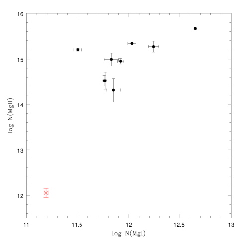
Figure 5: $\log N($Mg ii$)$ vs. $\log N($Mg i$)$ for the sample of DLA components collected by Dessauges-Zavadsky et al. (2006) and for the studied system component (cross).

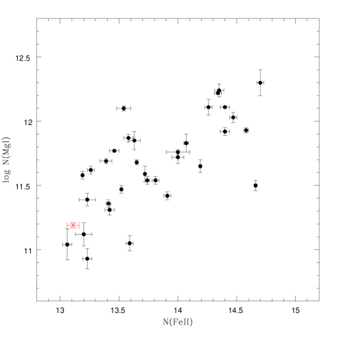
Figure 6: $\log N($Mg i$)$ vs. $\log N($Fe ii$)$ for the sample of DLA components collected by Dessauges-Zavadsky et al. (2006) and for the studied system component (cross).

DLA systems are characterized by the highest neutral hydrogen column density among QSO absorbers ($N($H i$)\geq 2\times 10^{20}$ cm^-2); however, up to now there are no detections of Fe i, Ca i, and Si i in those systems. Also, molecular hydrogen is not very common: it is present in about 13-20 percent of the presently observed DLA systems (Srianand et al. 2005). The coldest environments, rich in molecules and possibly in metals, could be missed by observations due to dust obscuring the background source.

We have compared the properties of our absorption system with the sample of 11 DLA by Dessauges-Zavadsky et al. (2006), where ionic column densities were measured component by component. Considering those components for which the column density were measured for at least two ions among Mg i, Mg ii, Mn ii, and Fe ii, we built a sample of 58 components. Figure 5 shows that, while the amount of Mg i observed in our system is comparable with that of the examined sample of DLA (see also Fig. 6), there is a difference of more than 2 orders of magnitude in the Mg ii column density, which, as shown in Sect. 3.1 cannot be ascribed to measurement uncertainties. On the other hand, we tend to exclude the possibility that Mg iii is the dominant ionization state in this system, due to the presence of the neutral elements. Now, if we look at Fig. 6, we see that the measured Fe ii column density is compatible with the lower values measured in the considered sample of DLA components. Note that in this plot there is a larger number of Mg i measurements than in Fig. 5, which is due to the fact that many systems with measured Mg i and Fe ii column densities have saturated (thus not measured) Mg ii lines.

The observed difference in the Mg i/Mg ii ratios could be due to a different ionization state in our system than the DLA population. However, the difficulty in measuring a precise column density for single Mg ii components in DLA due to saturation or blending may also play an important role.

Supposing that no ionization corrections are needed for our system, the abundance ratio with respect to solar of magnesium and iron (taking into account the contribution of all ionization stages) is [Mg/Fe] $\simeq-1.05\pm 0.05$, while the mean value for the considered sample of 11 DLA is $0.7\pm 0.4$. On the other hand, [Mn/Fe] $\simeq 0.31\pm 0.05$ at a variance with the DLA mean value $\simeq-0.23\pm 0.05$.

3.3 Comparison with local interstellar clouds

Another class of absorbers characterized by high neutral hydrogen column densities and showing some of the neutral transitions that we have measured is represented by the local cold interstellar clouds (Welty et al. 2003, WHM, and references therein).

We compared the properties of our system at $z\simeq 0.4521$ with the column densities for Ca i, Ca ii, and Fe i of local lines of sight towards star forming regions in Table 9 of WHM (excluding upper limits and uncertain determinations), while the H i column densities for the corresponding lines of sight are taken from Welty & Hobbs (2001, and references therein).

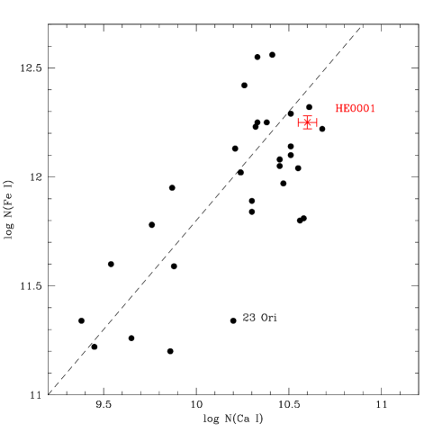
Figure 7: $\log N($Fe i$)$ vs. $\log N($Ca i$)$ for the sample of interstellar diffuse clouds collected in Welty et al. (2003) and for our QSO absorption system (cross). The dashed line indicates a linear relationship between the two species.

In Fig. 7 the column densities of Fe i vs. Ca i measured for the local interstellar medium are plotted with those of our absorber. The high-redshift value is in very good agreement with the local measurement and resides at the high column density tip of the distribution. The local absorption systems have neutral hydrogen column densities varying approximately between $\log N($H i$)\sim 20.5$ and $21.5$, with a slight correlation with the Ca i and Fe i column densities, indicating a high H i column density for our absorber. Allowing for that range of H i column densities and taking the observed total column density of (neutral plus singly ionized) Fe in our system, we estimated a range of metallicities, $-2.78\la$ [Fe/H] $\la-3.78$, lower than the lowest metallicities observed in DLA. At these Fe abundances, the effect of depletion onto dust grains should be negligible.

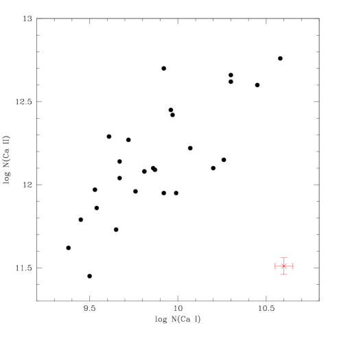
Figure 8: $\log N($Ca ii$)$ vs. $\log N($Ca i$)$ for the sample of interstellar diffuse clouds collected in Welty et al. (2003) and for the studied QSO absorption system (cross).

Figure 8 shows $\log N($Ca ii$)$ vs. $\log N($Ca i$)$ for the local sample and for our system. As in the case of Mg ii absorptions in DLA (see Fig. 5), there is a deficiency of Ca ii in our system with respect to the general distribution of interstellar clouds. A detailed analysis of single-component Ca i and Ca ii column densities in stellar spectra at very high resolution ($FWHM\sim 0.6-1.8$ km s^-1), shows that the average single component column density ratio is Ca i/Ca ii $\la-2$ (Pan et al. 2004). This result is a strong indication that the difference in Ca ii abundance between our system and the local interstellar clouds is due to a different ionization state.

4 Photoionization model

From the comparisons carried out in the previous sections, it is clear that our system shows some characteristics close to those of high H i column density absorbers. On the other hand, its ionization properties look different both from those of DLA and of local interstellar clouds.

We ran photoionization models with the version c06.02c of Cloudy (Ferland et al. 1998) to reproduce the observed ionization properties and investigate the physics of the studied cloud. We considered two types of radiation fields: a hard, QSO dominated spectrum representative of the UV background external to the system (as modeled by Madau, Haardt & Rees 1999, at $z=0.49$), and a soft, stellar-type spectrum ($T_{\rm eff}=33,000$ K, $\log g=4$; Kurucz 1991) representative of the internal radiation field or of an external field dominated by starlight from galaxies. A solar abundance pattern has been assumed and a metallicity, $Z$, computed from the observed Fe total column density and the adopted H i column density. The total density, thickness of the gas slab and H i column density are strictly related, $n_{\rm H}\times\Delta R\simeq N($H i$)$, since the investigated cloud is dominated by neutral gas. The first two parameters are constrained by observations. An upper limit on the size of the cloud of $\sim 150-200\,h^{-1}_{71}$ pc, comes from the study of single Mg ii components in spectra of lensed QSOs (Rauch et al. 2002). Molecular clouds associated with DLA in QSOs spectra have total densities $n_{\rm H}\simeq 10-200$ cm^-3 and temperatures $T\simeq 100-300$ K (Srianand et al. 2005), while, local cold interstellar clouds can be as small as a few parsecs, with total densities $n_{\rm H}\sim 10-15$ cm^-3 and temperature $T\sim 100$ K (e.g. Welty et al. 1999).

Taking the previous constraints into account, we ran a grid of photoionization models varying $n_{\rm H}$, $N($H i$)$, $Z$ and the ionization parameter

$$U\equiv\frac{\Phi_{912}}{c\,n_{\rm H}}=\frac{4\,\pi\,J_{912}}{h\,c\,n_{\rm H}}\simeq 2\times 10^{-5}\,\frac{J_{912}/10^{-21.5}}{n_{\rm H}/1\,\mbox{cm}^{-3}},$$ (1)

where $J_{912}$ is the intensity of the ionizing spectrum at the Lyman limit.

Table 2: Characteristic parameters and results of the photoionization models (see text).

Model	Spectrum	$\log N($H i$)$	$n_{\rm H}$	$\Delta R$	$Z$	$\log U_{\rm Mg}$	$\log J_{\rm Mg}$	$\log U_{\rm Ca}$	$\log J_{\rm Ca}$	(Fe i/Fe ii)max	Tmin
		cm-2	cm-3	pc		($\pm 0.03$)	($\pm 0.03$)	($\pm 0.05$)	($\pm 0.05$)		K
HM1	hard	20.7	10.0	15.0	-3.0	-6.62	-22.42	-7.56	-23.36	-2.81	110
STAR1	soft	20.7	10.0	15.0	-3.0	-6.66	-22.46	-7.36	-23.16	-2.80	110
HM2	hard	21.5	10.0	102.5	-3.8	-6.66	-22.46	-7.76	-23.56	-2.81	111
STAR2	soft	21.5	10.0	102.5	-3.8	-6.65	-22.45	-7.54	-23.34	-2.81	111
HM3	hard	21.5	63.1	15.0	-3.8	-6.95	-21.95	-7.93	-22.93	-2.71	83
STAR3	soft	21.5	63.1	15.0	-3.8	-6.95	-21.95	-7.71	-22.71	-2.71	83
HM4	hard	20.7	158.5	1.0	-3.0	-7.08	-21.68	-8.01	-22.61	-2.64	67
STAR4	soft	20.7	158.5	1.0	-3.0	-7.11	-21.61	-7.80	-22.40	-2.64	66
HM5	hard	21.5	1000.0	1.0	-3.8	-7.47	-21.27	-8.40	-22.20	-2.61	62
STAR5	soft	21.5	1000.0	1.0	-3.8	-7.49	-21.29	-8.19	-21.99	-2.62	61

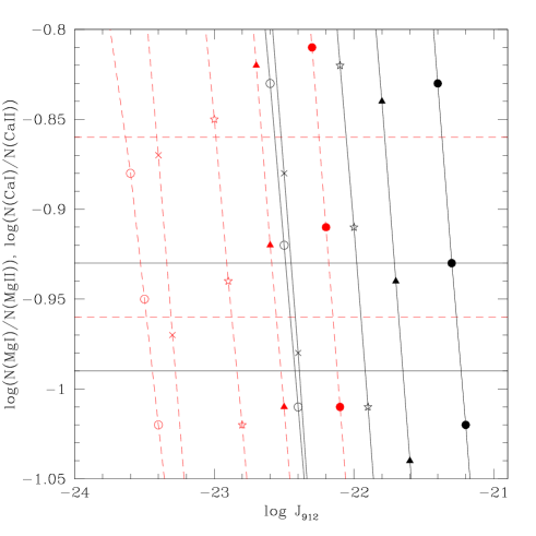
Figure 9: $\log(N($Mg i$)/N($Mg ii$))$ (solid lines) and $\log(N($Ca i$)/N($Ca ii$))$ (dashed lines) as a function of the log of the Lyman limit intensity of the ionization spectrum for the 5 test photoionization model run with Cloudy (see Table 2) in the case of the hard spectrum. The legend of symbols is the following: cross - Model 1, empty circle - Model 2, star - Model 3, solid triangle - Model 4, solid circle - Model 5. The solid and dashed horizontal lines delimit the 1 $\sigma$ interval of the observed values for $\log(N($Mg i$)/N($Mg ii$))$ and $\log(N($Ca i$)/N($Ca ii$))$, respectively.

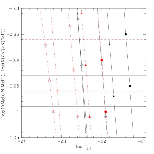
Figure 10: Same as Fig. 9 but for the stellar ionizing spectrum.

The parameters of the five physical models that we studied in detail, adopting both the hard and soft ionizing spectra, are reported in Table 2, together with the values of the ionization parameter, $U$, and the corresponding ionizing flux at the Lyman Limit, $J$, at which we obtained the observed values for $\log(N($Mg i$)/N($Mg ii$))$ and $\log(N($Ca i$)/N($Ca ii$))$. In columns 11 and 12, we also report the maximum value obtained for the $\log(N($Fe i$)/N($Fe ii$))$ ratio and the corresponding minimum temperature reached for that model. We stopped when a further decrease in $U$ did not correspond to a decrease in $T$.

Model by model, the main difference due to the different ionizing spectrum is the value of the ionization parameter at which we obtained the observed column density ratio for Ca, which is a factor $\sim 1.6$ systematically higher for the soft spectrum. As expected, the lower temperatures are reached in the region far away from the ionizing source and strongly depend on the adopted total density. The Fe column density ratio is tightly related to the lowest temperature reached (about 60 K), and we could not obtain values of $\mbox{Fe\,{\sc i}}/\mbox{Fe\,{\sc ii}}$ higher than $\simeq 0.0024$ or about 55 times lower than the observed value. In Figs. 9, 10 we report the obtained $\log N($Mg i$)/N($Mg ii$)$ and $\log N($Ca i$)/N($Ca ii$)$ as a function of the intensity at the Lyman limit of the hard and soft ionizing spectra. Higher intensities are needed for denser clouds. There is a range of intensities for both ionizing spectra, $-22.45\la\log J_{912}\la-21.95$, at which the observed $\log N($Mg i$)/N($Mg ii$)$ and $\log N($Ca i$)/N($Ca ii$)$ are reproduced. Neutral and singly ionized Mg arise in clouds with total density $n_{\rm H}=10$ or $\sim 63.1$ cm^-3 and Ca in clouds with $n_{\rm H}\simeq 158.5$ or $1000$ cm^-3, respectively. The above range of $J_{912}$ agrees closely with the intensity of the UV background measured at $z<1$ from the QSO proximity effect, $-22.3\la\log J_{912}\la-21.98$ (Scott et al. 2002).

For comparison, the average $\log N($Ca i$)/N($Ca ii$)$ ratio observed for local interstellar clouds is obtained for $\log J_{912}\sim-22$ in the case of a cloud of 15 pc and $n_{\rm H}=10$ cm^-3. It is interesting to note that the 2nd main ionization state of Ca in this conditions is Ca iii, while at the ratio observed in our system it is Ca i.

The main result of our calculations is that we could not find any combination of the parameters resulting in a model that could reproduce the three observed ratios at the same time: $N($Mg i$)/N($Mg ii$)$, $N($Ca i$)/N($Ca ii$)$, and $N($Fe i$)/N($Fe ii$)$. We can infer that the UV background is likely to be the ionizing source of the observed gas; however, simple photoionization models with uniform density cannot explain the observations and more complex density structures should be adopted.

5 Conclusions

We report the study of a very peculiar metal absorption system detected in the UVES spectrum of the QSO HE0001-2340 at $z\simeq 0.452$.

The system is characterized by a single narrow component in Mg ii and is classified as a weak Mg ii absorber. However, at the same redshift we also observed transitions due to Mg i, Ca ii, Mn ii, Fe ii and, in particular, to Si i, Ca i, Fe i, which are observed for the first time in a QSO absorption system. The difference between the properties of our system and those of the sample of weak Mg ii systems that we have collected in the ESO Large Programme QSO spectra gives an estimate of the probability of intersecting such a cloud: we observed one over 34 (single Mg ii components), or $P\approx 0.03$.

The presence of rare neutral elements suggests that the gas is shielded by a large amount of neutral hydrogen, so we have compared its chemical properties with those of the highest H i column density QSO absorptions, the damped Lyman-$\alpha$ systems, and with the local cold interstellar clouds. The main results deriving from this comparison are the following.

1. The ratios Mg i/Mg ii  and Ca i/Ca ii  are at least two and one orders of magnitude higher in our system than in the other absorbers. A large fraction of doubly ionized Mg and Ca is excluded by the presence of the rare neutral species. It has to be noted that there are only a few measures of Mg ii in DLA (see Dessauges-Zavadsky et al. 2006); and in general, both in DLA and local interstellar clouds, Mg ii and Ca ii are more extended than the corresponding Mg i and Ca i, implying that they are due to more extended regions. However, in very high-resolution stellar spectra, the Ca i/Ca ii  ratio computed component-by-component is still one order of magnitude lower than in our system, strongly suggesting that our system has a lower ionization state.

2. We can give a rough estimate of the metallicity by assuming that our system has an amount of H i comparable to what observed in local interstellar clouds with similar abundances of Ca i and Fe i. This implies a range of metallicities $-2.78\la$ [Fe/H] $\la-3.78$, lower than the lowest metallicities measured in DLA.

3. More puzzling is the underabundance of Mg with respect to Fe, which is very hard to explain both with nucleosyntesis and with differential dust depletion. Indeed, interstellar cold clouds generally show significantly larger Fe depletion than Mg depletion (e.g. Savage & Sembach 1996).

We studied the physical and ionization properties of our cloud by running a grid of photoionization models with Cloudy. It is not possible to recover the observed Mg i/Mg ii, Ca i/Ca ii, and Fe i/Fe ii column density ratios with a single gas slab of constant density. On the other hand, by adopting an ionizing spectrum compatible with the UV background at $z<1$, the correct Mg and Ca ratios are obtained in gas with a total density of $n_{\rm H}\sim 10-60$ and $150-1000$ cm^-3, respectively. The Fe ratio cannot be reproduced, but there are indications that gas denser than $n_{\rm H}\sim 1000$ cm^-3 is needed. These results suggest that only a complex density structure for the cloud could explain the observed ionic abundances.

What is this very rare cloud? A definite answer could come from UV observations of this object to measure the H i and the H₂. Furthermore, a better search for these class of systems would be possible with spectrographs at a higher resolving power ($>100\,000$) than presently provided by instruments like UVES and HIRES on 8-10m class telescopes.