Mixing navigation on networks

Abstract

In this Letter, we proposed a mixing navigation mechanism, which interpolates between random-walk and shortest-path protocol. The navigation efficiency can be remarkably enhanced via a few routers. Some advanced strategies are also designed: For non-geographical scale-free networks, the targeted strategy with a tiny fraction of routers can guarantee an efficient navigation with low and stable delivery time almost independent of network size. For geographical localized networks, the clustering strategy can simultaneously increase the efficiency and reduce the communication cost. The present mixing navigation mechanism is of significance especially for information organization of wireless sensor networks and distributed autonomous robotic systems.

Information navigation is the fundamental function of all communication networks. There are two kinds of information: The nonspecific one, of relevance to broadcasting process, epidemic spreading and rumor propagation, is desirous to travel all over the networks, while the specific information focus only on locating one targeted node. Here we concentrate on the latter case. In a decentralized file-sharing system, such as GNUTELLA and FREENET, files are found by forwarding queries to one’s neighbors until arriving the target Adamic2001 . Without any navigation, to find a file in those systems is equivalent to a random-walk search, which is inefficient in large-size networks Adamic2001 ; Noh2004 . The navigation efficiency can be sharply improved by using some local information, such as the geographical location of target Kleinberg2000 , the degrees of neighboring nodes Adamic2001 ; Kim2002 , and local betweenness centrality (LBC) Thadakamalla2005 . In an extreme case, if all the nodes know how to deliver the message along with the shortest path, the highest efficiency can be achieved with delivery time being equal to the shortest path-length. However, this ideal navigation system is impractical in huge-size networks since it requires either a great amount of external information Trusina2005 or a huge memory of each node Rosvall2003 , which costs too much. Especially, in many real communication networks, such as Limewire, Kazaa and eDonkey, the edges can be rapidly rewired Cholvi2005 . For the economical and technical reasons, it is hard to design a navigation system where each node has enough power to detect the structural or geographical changes, as well as strong computational ability to dynamically find the shortest paths.

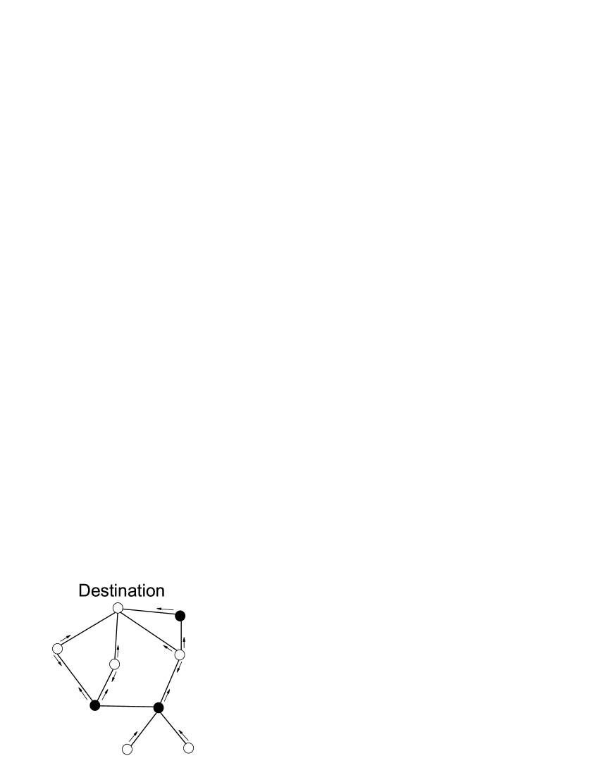
Figure 1: Mixing navigation on networks. The network consists of two kinds of nodes, forwarders (hollow circles) and routers (solid circles). As a holder, the forwarder will forward the message to a randomly selected neighbor, while the router can deliver it one step towards its destination. The arrows located in each node represent the possible delivering directions for the given destination.

Many efforts have been made previously on finding highly effective navigation algorithm with low communication cost. In those studies, a latent and maybe oversimple assumption is that all the nodes in the network are functionally equivalent. In this Letter, we raise a partially centralized navigation system where a tiny fraction of nodes, called routers, know where the shortest path is, while most nodes, called forwarders, can only randomly forward the message to one of their neighbors. This mixing navigation mechanism is practicable and necessary in some significant self-driven systems. Consider a wireless sensor network Akyildiz2002 ; Oqren2004 ; its topology varies dynamically due to the power-exhaustion of some sensors as well as the changing of frequency channels for security reason. Since the power of each sensor is limited, it can not be a router especially for long time. A possible way is that each sensor behaves as a router for a short period (peer-to-peer way), or, a very few specific sensors are previously given more power and will be the routers (partially centralized way). Another typical example is the distributed autonomous robotic system Arai2002 , where each robot moves fast and the direct communication can only be carried out within a limited horizon like the Vicsek model Vicsek1995 . A router must have the ability to detect the location of target, thus can send the message in the right direction Kleinberg2000 . Overmany routers bring high economic pressure, while without routers the communication will be inefficient. We expect the embedding of a tiny fraction of routers could guarantee both the high efficiency and the low cost to the system. This idea is also inspired by the collective phenomenon of biological swarm, in which a very few effective leaders can well organize the whole population Couzin2005 .

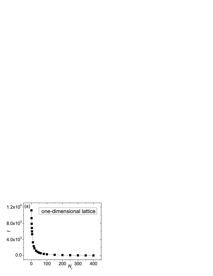
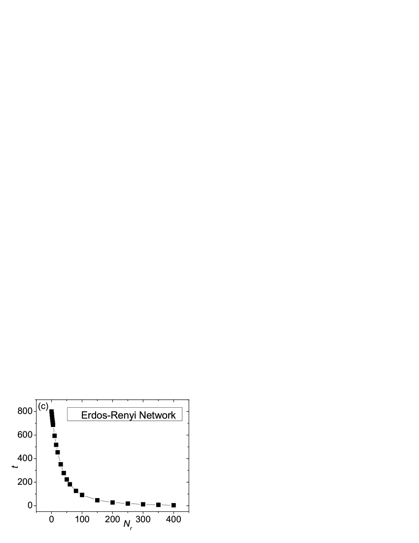
Figure 2: Expected delivery time $t$ vs. $N_{r}$ with random selection of routers in (a) one-dimensional lattice, (b) two-dimensional lattice, (c) Erdös-Rényi (ER) networks Erdos1959 , (d) Watts-Strogatz (WS) networks Watts1998 . The lattices are of periodic boundary conditions, and the WS network is generated from one-dimensional lattice with rewiring probability $p=0.1$. In all those networks, the size $N=400$ and average degree $\langle k\rangle=4$ are fixed. All the data points are obtained by averaging over $10^{6}$ independent runs.

The primary figure of merit for the present model is the expected delivery time $t$, which represents the expected number of steps (hop-counts) needed to deliver a message from a random source to a random destination (see Fig. 1 the rule of mixing navigation). Taking into account the different measures of cost, we divide the underlying networks into two classes: One is non-geographical networks, where the Euclidean coordinates of nodes and the lengths of edges have no physical meaning (e.g. World-Wide-Web, metabolic networks, etc.). The other is geographical networks having well defined node locations (e.g. wireless sensor networks, distributed robotic networks, etc.). In the former case, the cost of router mainly results from the hardware implementation, since each router needs a large memory to store the routing table Yan2006 ; ex . Therefore, the number of routers, $N_{r}$, is directly used to approximately measure the cost. In the latter case, usually, the nodes are moving continuously; since the direct communication is often bounded with a radius $r_{c}$, the router has to find out the location of target, as well as the locations of all its neighboring nodes with distance $<r_{c}$. This operation can be implemented by sending a signal (not message) through a specific frequency channel to all other nodes and analyzing the feedback, which requires certain amount of power. Therefore, to save power, the router may switch its working mode to a simple forwarder sometimes. The cost, concerning power only Akyildiz2002 , can be measured by the total time working as a router.

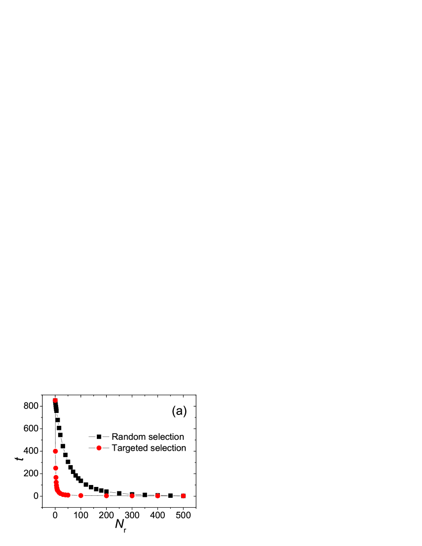
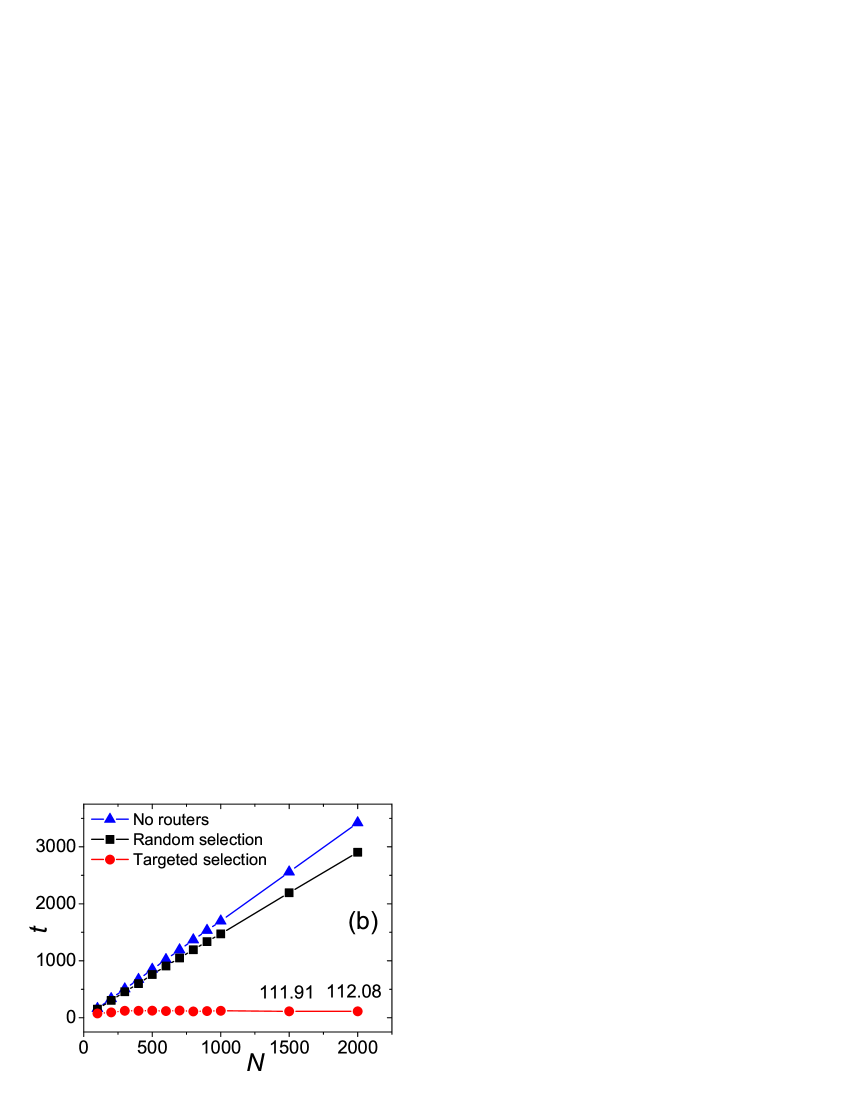
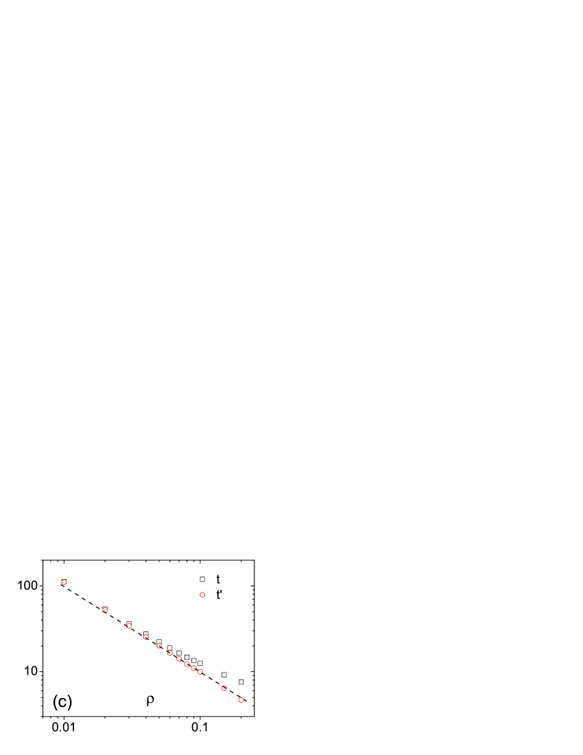
Figure 3: (color online) (a) Expected delivery time $t$ vs. $N_{r}$ with random selection (black square) and targeted selection (red circle) on BA networks with size $N=500$ and average degree $\langle k\rangle=6$. (b) Scaling behavior of $t$ as the increasing of $N$. The average degree $\langle k\rangle=6$ and router density $\rho=N_{r}/N=0.01$ are fixed. The values of the last two points in targeted selection is marked. The data points in the two upper curves can be linearly fitted with slope $1.714\pm 0.002$ and $1.447\pm 0.007$, respectively. (c) Expected delivery time $t$ (black square) and rescaled delivery time $t^{\prime}$ (red circle) as a function of $\rho$. The straight line is of slope -1. The network is of $N=2000$ and $\langle k\rangle=6$. All the data points in (a), (b) and (c) are averaged over $10^{7}$ independent runs.

We start with a trivial method, namely random selection, where a few nodes are randomly selected to be routers. Fig. 2 reports the simulation results of some homogenous networks. The expected delivery time $t$ remarkably decreases after the addition of a tiny fraction of routers. Then, when $N_{r}$ gets larger, the decreasing speed, $-\partial t/\partial N_{r}$, becomes slower and the saturation is clearly observed.

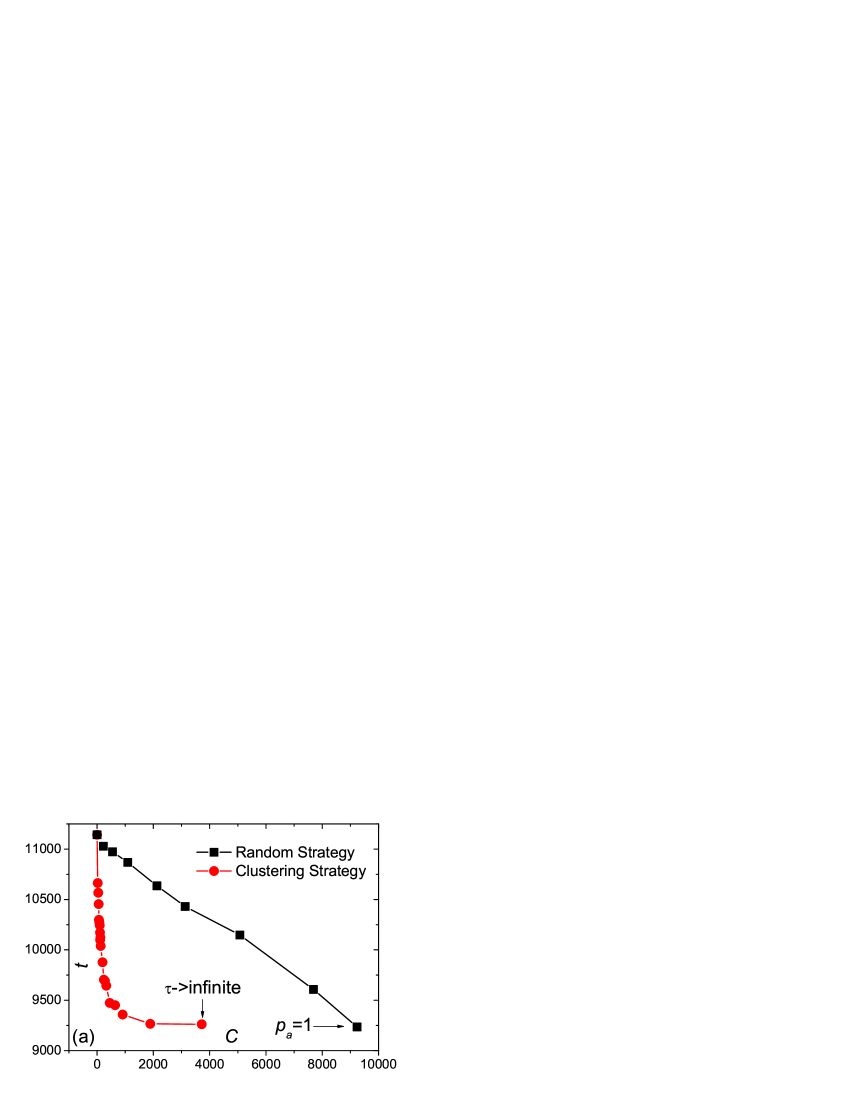
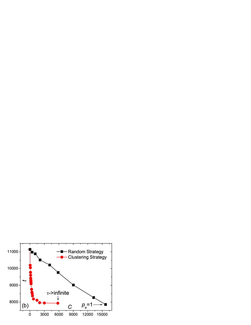
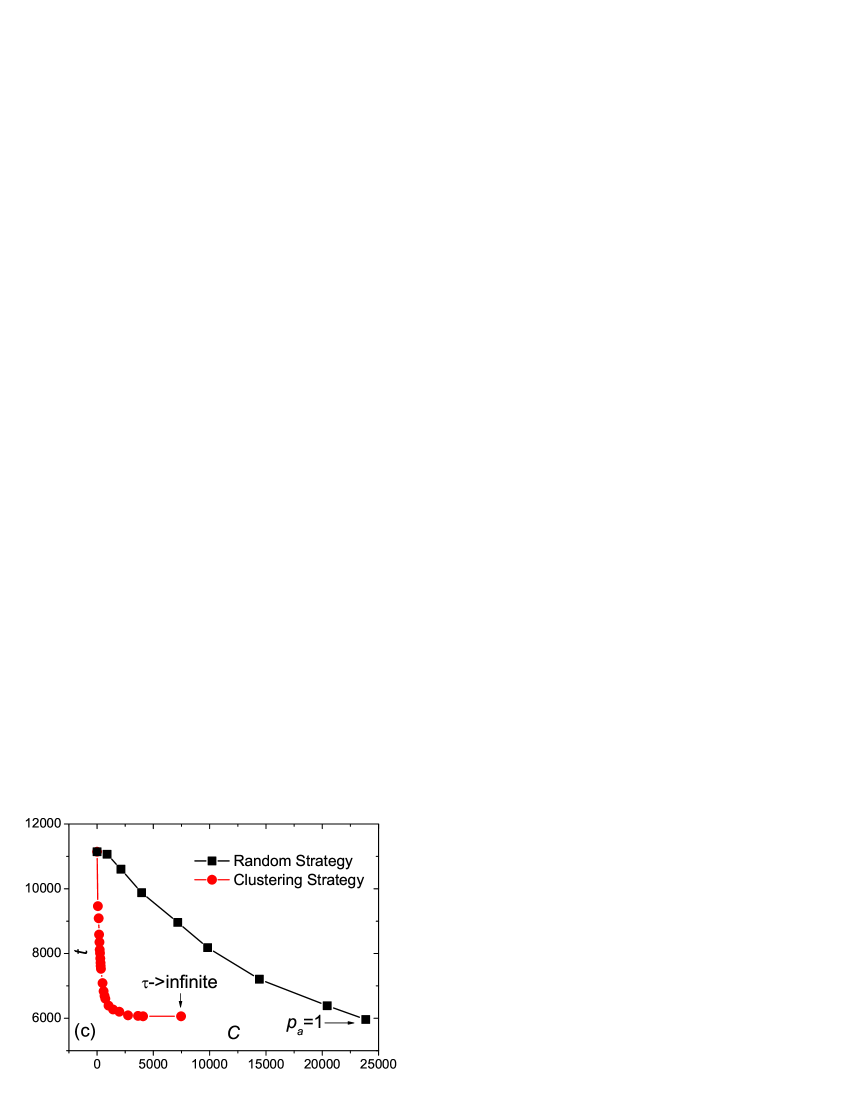
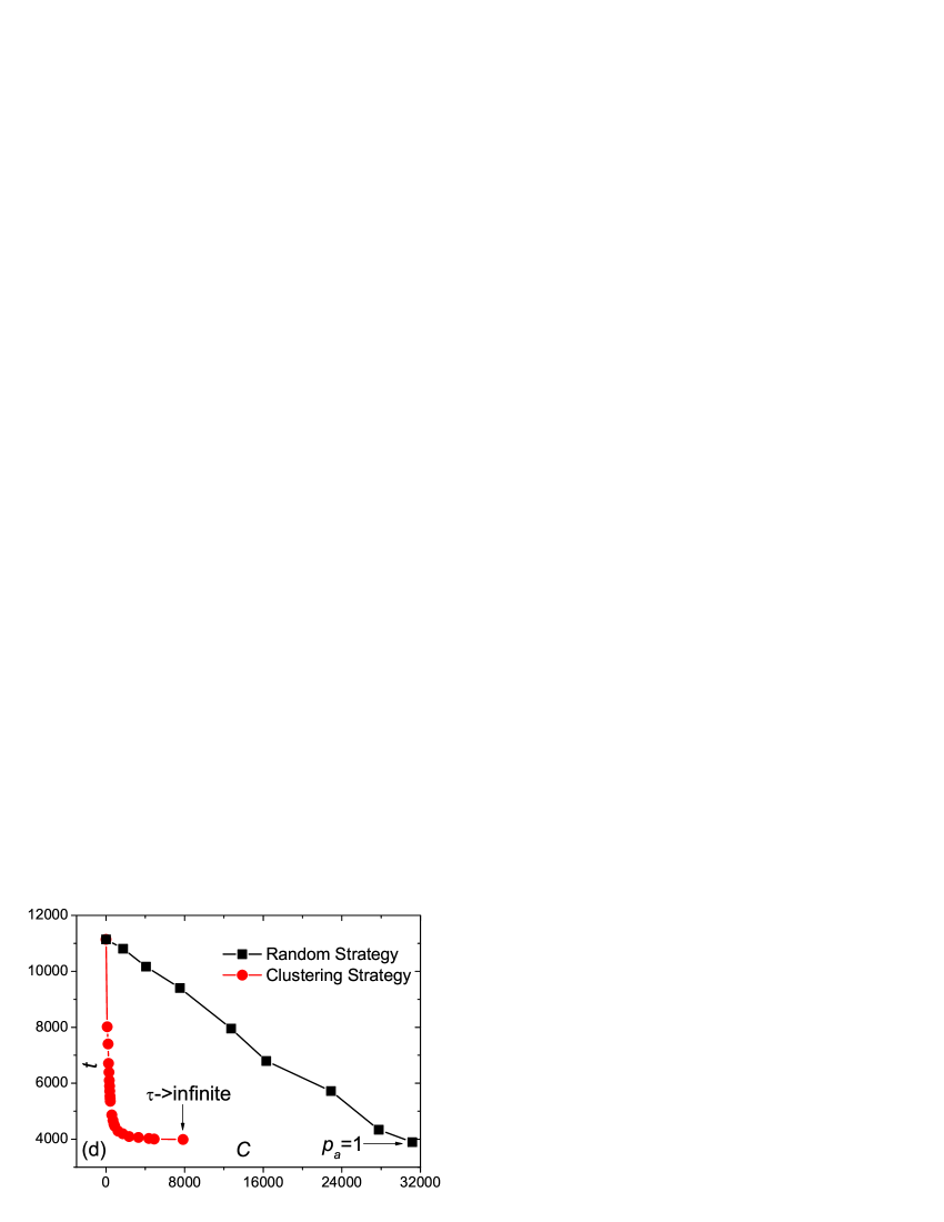
Figure 4: (color online) Expected delivery time $t$ as a function of cost $C$ on one-dimensional lattice. The number of routers are $N_{r}=1$ (a), 2 (b), 4(c) and 8 (d), respectively. The $t-C$ relations for random and clustering strategies are obtained by tuning $\tau$ in $[1,\infty)$ and $p_{a}$ in $[0,1]$, respectively. $\tau\rightarrow\infty$ means the router will never return to inactive state after it becomes active. $t(\tau\rightarrow\infty)$ is slightly larger than $t(p_{a}=1)$ since in the former case when a message visits a router in the first time, it will be randomly forwarded. The network size $N=400$ and average degree $\langle k\rangle=4$ are fixed. All the data points are obtained by averaging over $10^{6}$ independent runs.

Since the majority of real non-geographical networks have heterogenous degree distribution Albert2002 , we next implement this model onto the Barabási-Albert (BA) networks Barabasi1999 . Inspired by the prior studies on attack Albert2000 ; Cohen2001 and immunization Pastor-Satorras2002 , we propose a targeted selection strategy where $N_{r}$ nodes with the highest degree are selected to be routers. As shown in Fig. 3a, compared with the random selection strategy, the targeted one has much higher efficiency. With one router added, the delivery time $t$ drops to its half, and the efficiency can be enhanced about 10 times via only 5 routers. Fig. 3b shows the delivery time as a function of network size. Without any routers, $t$ scales linearly with $N$, and a small fraction of randomly added routers will not change its scaling behavior, but only reduce the growing rate $\partial t/\partial N$. Surprisingly, under the targeted strategy, even a very tiny fraction (e.g. $\rho=0.01$) of routers can guarantee a highly efficient navigation with $t$ almost stable as the increasing of system size. The scaling behavior can be analytically predicted in the large-size limit $N\rightarrow\infty$. If $\rho=0$, the current navigation algorithm degenerates to random walk with $t\sim N$ ex2 , and for any $\rho$ larger than the percolation threshold Callaway2000 , the network is decomposed into many interconnected forwarder-cores bounded with routers, and the delivery time consists of two parts: One accounts for the time randomly walking inside the cores, the other for the time travelling along with the boundary from the core containing the source to that containing the destination. Approximately, the former scales as $t_{1}\sim 1/\rho$, while the latter is approximated to $t_{2}\approx\langle l\rangle(1+\texttt{log}^{\rho}_{N})$, where $\langle l\rangle$ denotes the average shortest path-length. When $\rho$ is very small (close to $1/N$), the contribution of $t_{2}$ is neglectable even for huge (but not really infinite) $N$ , thus $t\approx t_{1}\sim 1/\rho$. As shown in Fig. 3c, in the log-log plot, $t(\rho)$ can be fitted by a straight line with slope -1 for very small $\rho$. However, when $\rho$ gets larger, the departure from $\rho^{-1}$ scaling becomes visible. To move out the contribution of $t_{2}$, we use a rescaled delivery time $t^{\prime}=t-\langle l\rangle(1+\texttt{log}^{\rho}_{N})$, which can be well fitted by a straight line with slope $-1.002\pm 0.005$ in the interval $\rho<0.3$. When $\rho$ goes close to 1, $t_{2}$ will be dominant thus $t\sim\texttt{ln}N$, as what we expect in the shortest-path searching algorithm. The details of analyses will be published in an extending paper.

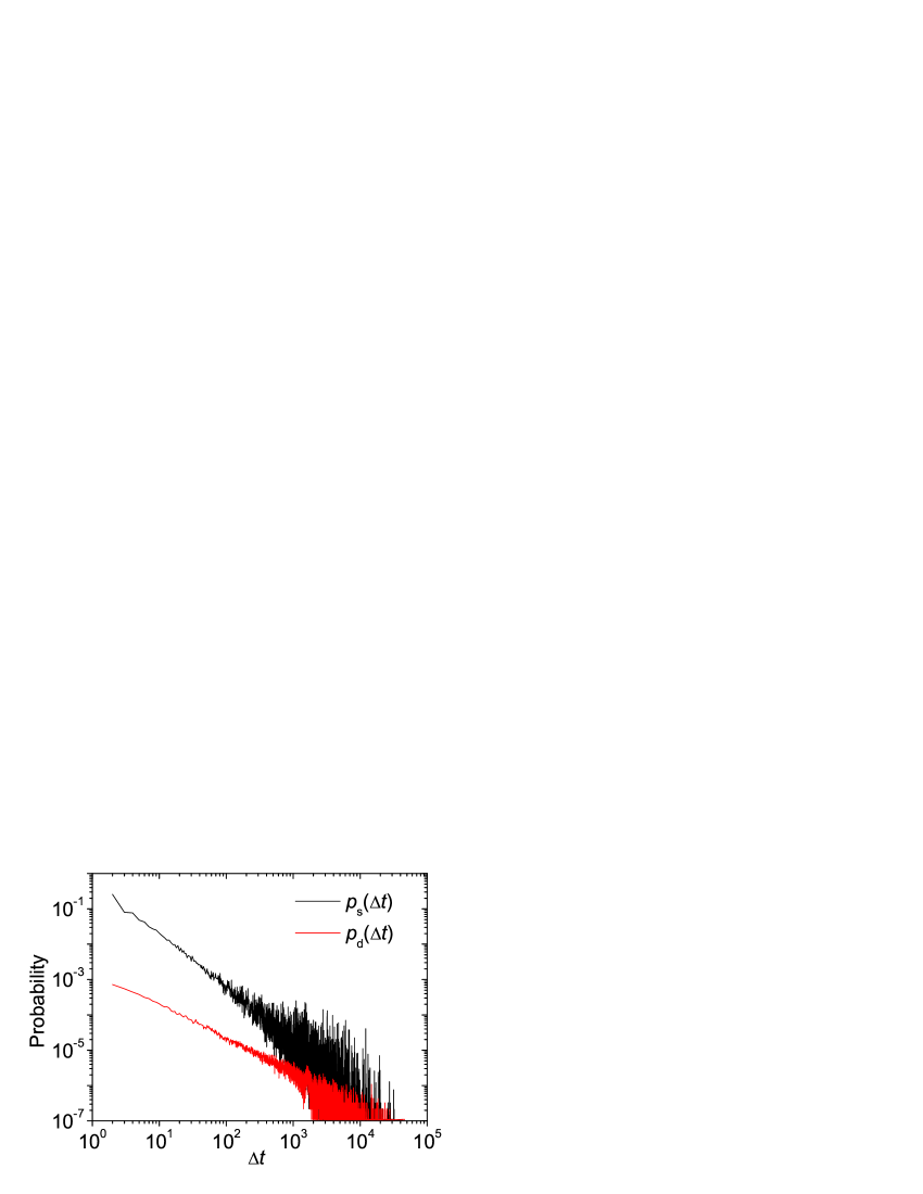
Figure 5: (color online) The time-correlated hitting probability $p_{s}$ and $p_{d}$ as a function of time interval $\Delta t$. The simulation results are averaged over $10^{7}$ independent runs, for a one-dimensional lattice with $N=400$, $N_{r}=2$ and $\langle k\rangle$=4.

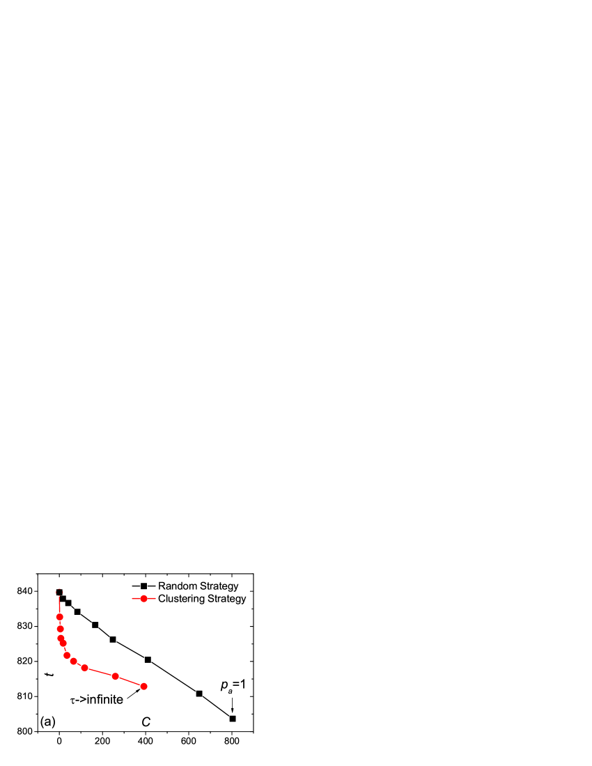
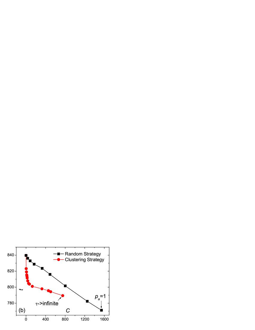
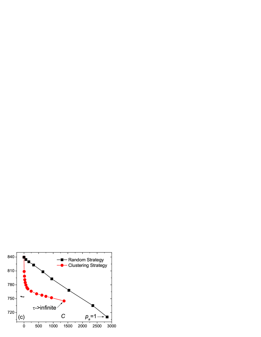
Figure 6: (color online) $t$ vs. $C$ on two-dimensional lattice. The setting of $N$, $N_{r}$ and $\langle k\rangle$ are the same as those of Fig. 4.

We next explore the navigation on geographical networks. For simplicity, the network is embedded in a one-dimensional lattice with periodic boundary condition, and the average degree, which reflects the horizon $r_{c}$, is fixed as $\langle k\rangle=4$. The routers are randomly distributed in the network, each of which can be in one of the two states: active or inactive. In the former state, the router will continuously send/recieve specific signals to detect the locations of all other nodes thus can delivery the message one step towards its destination. In the latter state, the router behaves like a simple forwarder. The cost, denoted by $C$, is measures by the total active time summing over all the routers. The transmit time from one node to its neighbor is assumed to be the same for any message, and counted as the system time unit. The simplest strategy is to switch randomly, that is to say, at each time step, each router will be active with probability $p_{a}$, where $p_{a}$ is a constant independent of time. Given network structure and the number of routers, both the delivery time $t$ and the cost $C$ are statistically determined by $p_{a}$, thus by tuning $p_{a}$, a curve in $t-C$ (efficiency-cost) plane can be obtained. Moreover, we propose a novel switching method, namely clustering strategy. In this strategy, if an inactive router receives a message at time step $T$, it will forward it to a random neighbor and then becomes active from time $T+1$ to $T+\tau$. For an active router, it will send this message one step along with the shortest path to the destination, and keep active from time $T+1$ to $T+\tau$. If this message will not come again before $T+\tau$, the router switches to inactive. Initially, all the routers are inactive. Analogously, by adjusting $\tau$, a curve in the efficiency-cost plane can be obtained.

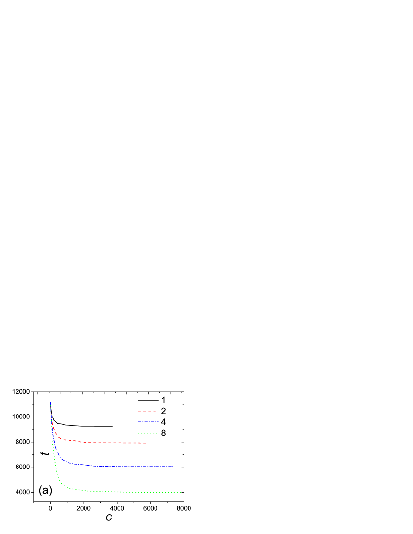
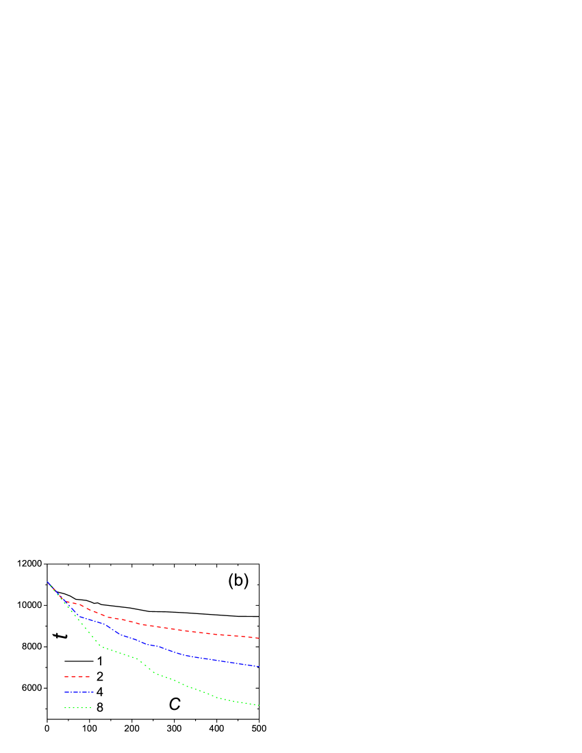
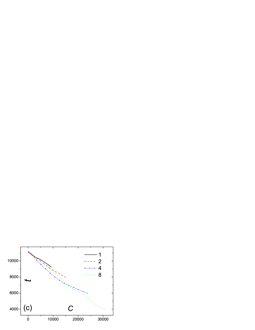
Figure 7: (color online) The relations between $t$ and $C$ for $N_{r}=1$ (black solid), 2 (red dash), 4 (blue dash-dot) and 8 (green dot) under clustering strategy (a) and random strategy (c), respectively. The panel (b) illustrates the part of (a) for small $C$. The data shown here are obtained from the same simulation environment as that of Fig. 4.

The simulation results for random and clustering strategies are shown in Fig. 4. Clearly, by raising the cost (i.e., increasing $p_{a}$ and $\tau$, respectively), the navigation efficiency can be enhanced. With the same cost, the clustering strategy performs much better than random strategy. It is because the track of message has a localized effect (also called the phenomenon of information clustering). Generally, after visiting a router $i$, a message will walk within $i^{\prime}s$ surrounding area during a certain time period, with much higher probability hitting $i$ again than other “far away” routers. To measure this localized effect, we introduce a time-correlated hitting probability $p(\Delta t)$, which is defined as the probability that the time interval of two sequent hits is $\Delta t$, where a hit means the message arriving at a router. Divide $p(\Delta t)$ into two parts $p(\Delta t)=p_{s}(\Delta t)+p_{d}(\Delta t)$, where $p_{s}(\Delta t)$ ($p_{d}(\Delta t)$) denotes the case if two sequent hits are on the same router (different routers). Fig. 5 reports the simulation results of $p_{s}$ and $p_{d}$ in one-dimensional lattice. Clearly, for small $\Delta t$, $p_{s}$ is $>2$ orders of magnitude larger than $p_{d}$, indicating the strongly localized effect. Therefore, the clustering strategy simultaneously has two advantages: Firstly, it increases the probability that a router is active when being revisited, thus can enhance the efficiency; on the other hand, it avoids the useless activities of some “far away” routers, thus can hold down the cost. Fig. 6 reports the simulation results about $t-C$ relations on two-dimensional lattice with periodic boundary condition, which also demonstrate the visible advantage of clustering strategy. However, the improvement from random to clustering strategy in the two-dimensional lattice is smaller than that in one-dimensional case. Actually, the advantage of clustering strategy is more remarkable in more localized networks. In geographical lattice, the one having larger scale $N^{1/d}$ and smaller horizon $r_{c}$ is more localized, where $d$ denotes the dimension.

Clearly, better efficiency can be achieved by adding more routers. However, it may also increase the cost. As shown in Fig. 7c, for the case of random strategy, the four curves for different $N_{r}$ have almost the same decaying rate. Therefore, if using the decrement of $t$ resulting from unit cost to judge the strategy, the addition of routers can not enhance the performance of random strategy. This finding is hackneyed in many real situation: Given a strategy, if one wants to gain more, one has to pay more. Interestingly, it is found that the performance of clustering strategy can be enhanced by adding more routers. As shown in Fig. 7a and Fig. 7b, the decaying rate of larger-$N_{r}$ curve is remarkably higher than that of smaller-$N_{r}$ curve, indicating that the clustering strategy with larger $N_{r}$ can bring more improvement via unit cost. Although only the cases $N_{r}=1,2,4,8$ are plotted, this conclusion is valid for all $N_{r}=1,2,\cdots,N$. For example, in the extreme case $N_{r}=N=400$, to reduce delivery time to $t\approx 150$ only costs $C\approx 375$.

In conclusion, the efficient of mixing navigation in non-geographical networks is strongly related to the percolation problem. When $p$ exceeds the percolation threshold, the underlying network will be decomposed into many small-size forwarder-cores, guaranteeing the short delivery time. It is the reason why the targeted strategy can give rise to a highly efficient navigation with very low communication cost. For geographical networks, taking into account the information localization, we proposed a clustering strategy, whose advantage is more remarkable in more localized networks. The strength of localization can be measured by the ratio $p_{s}/p_{d}$, the higher ratio indicates the stronger localized effect. Since the hardware cost of single sensor drops exponentially and power supply becomes the bottleneck of well communication in huge-size wireless sensor networks, the clustering strategy, especially the extreme case $N_{r}=N$, is of significant importance in practice.

This work is support by the NNSFC under Grant Nos. 10635040 and 10472116.

References

- (1) L. A. Adamic, et al., Phys. Rev. E 64, 046135 (2001).
- (2) J. D. Noh, and H. Rieger, Phys. Rev. Lett. 92, 118701 (2004).
- (3) J. M. Kleinberg, Nature 406, 845 (2000).
- (4) B. J. Kim, et al., Phys. Rev. E 65, 027103 (2002).
- (5) H. P. Thadakamalla, et al., Phys. Rev. E 72, 066128 (2005).
- (6) A. Trusina, et al., Phys. Rev. Lett. 94, 238701 (2005).
- (7) M. Rosvall, and K. Sneppen, Phys. Rev. Lett. 91, 178701 (2003).
- (8) V. Cholvi, et al., Phys. Rev. E 71, 035103(R) (2005).
- (9) I. F. Akyildiz, et al., Computer Networks 38, 393 (2002).
- (10) P. Oqren, et al., IEEE Trans. Automat. Contr. 49, 1292 (2004).
- (11) T. Arai, et al., IEEE Trans. Robot. Automat. 18, 655 (2002).
- (12) T. Vicsek, et al., Phys. Rev. Lett. 75, 1226 (1995).
- (13) L. D. Couzin, et al., Nature 433, 513 (2005).
- (14) G. Yan, et al., Phys. Rev. E 73, 046108 (2006).
- (15) Each router should store the identifications of neighboring nodes on the shortest path to each potential destination (see also the memory of each agent in Ref. Rosvall2003 ), which requires at least integral memory.
- (16) P. Erdös, and A. Rényi, Publ. Math. 6, 290 (1959).
- (17) D. J. Watts and S. H. Strogatz, Nature 393, 440 (1998).
- (18) R. Albert, and A. -L. Barabási, Rev. Mod. Phys. 74, 47 (2002).
- (19) A. -L. Barabási and R. Albert, Science 286, 509 (1999).
- (20) R. Albert, et al., Nature 406, 378 (2000).
- (21) R. Cohen, et al., Phys. Rev. Lett. 86, 3682 (2001).
- (22) R. Pastor-Satorras, and A. Vespignani, Phys. Rev. E 65, 036104 (2002).
- (23) For a scale-free network with degree distribution , the expected delivery time of a random-walk navigation scales as , since for BA networks, , sacles linearly with the network size .
- (24) D. S. Callaway, et al., Phys. Rev. Lett. 85, 5468 (2000).